1 Introduction
Reactive mass transport processes in porous media are fundamental in many areas of subsurface science and engineering. For example, underground cave systems result from the dissolution of minerals by acidic solutions that flow through the porous subsurface geological formations. Although dissolution processes are local phenomena, their consequences span a wide range of time and length scales. The chemical dissolution of carbonate rocks may form sinkholes that vary in size from 1 to 600 m in diameter. Good understanding of the dissolution processes is particularly important to assess the long-term integrity of underground storage formations following the injection of carbon dioxide into deep saline aquifers (Rathnaweera, Ranjith & Perera Reference Rathnaweera, Ranjith and Perera2016). Indeed, the
 $\text{CO}_{2}$
makes the in situ brine more acidic, and that can enhance the reaction with the solid; the results can produce leakage pathways that threaten the integrity of the storage system (Steefel, Molins & Trebotich Reference Steefel, Molins and Trebotich2013). The injection of acid in carbonate formations is a widely used technique to stimulate the production capacity of wells. Acid injection is thought to be effective at removing ‘damage’ in the vicinity of the wellbore; moreover, the dynamic acid injection process may lead to the formation of preferential fluid-flow channels (wormholes) (Williams, Gidley & Schechter Reference Williams, Gidley and Schechter1979). Acid stimulation techniques are expected to increase the permeability of enhanced geothermal systems, while minimizing the level of induced seismicity (Portier et al.
Reference Portier, Vuataz, Nami, Sanjuan and Gérard2009). In practice, the flow regime and the density of the resulting fingers – wormholes – depend on several parameters, including the injection rate. Thus, better understanding of the dissolution dynamics can improve our ability to estimate the injection rate in order to maximize the benefits of the acid injection.
Dissolution patterns take different forms according to the flow conditions and the mineral properties (Daccord Reference Daccord1987; Daccord & Lenormand Reference Daccord and Lenormand1987; Daccord, Lietard & Lenormand Reference Daccord, Lietard and Lenormand1993; Fredd & Fogler Reference Fredd and Fogler1998a ,Reference Fredd and Fogler b ; Golfier et al. Reference Golfier, Zarcone, Bazin, Lenormand, Lasseux and Quintard2002; Szymczak & Ladd Reference Szymczak and Ladd2009; Soulaine et al. Reference Soulaine, Roman, Kovscek and Tchelepi2017). Dissolution of a natural formation is highly nonlinear and involves complex interactions of reactions, advection and diffusion. For example, the injection of acid in a tight (low-permeability) carbonate formation at high flow rate generates instabilities that ultimately evolve into ramified large-scale wormholes. At flow rates that are low enough, the transport is dominated by diffusion, and the dissolution process is characterized by a very stable fluid front (Golfier et al. Reference Golfier, Zarcone, Bazin, Lenormand, Lasseux and Quintard2002; Szymczak & Ladd Reference Szymczak and Ladd2009; Soulaine et al. Reference Soulaine, Roman, Kovscek and Tchelepi2017). Experimental observations suggest strong coupling between buoyancy effects, convective transport and kinetically controlled reactions (Oltéan, Golfier & Buès Reference Oltéan, Golfier and Buès2013). The highly nonlinear and complex nature of the different dissolution regimes make it practically impossible to fully understand the dynamics based on a Darcy-scale representation. For example, the evolution of the pore space can be quite different for the different dissolution regimes, and that prevents the use of a universal model to represent the relationship between porosity and permeability (Békri, Thovert & Adler Reference Békri, Thovert and Adler1995; Varloteaux, Békri & Adler Reference Varloteaux, Békri and Adler2013a ; Huber, Shafei & Parmigiani Reference Huber, Shafei and Parmigiani2014; Kang et al. Reference Kang, Chen, Valocchi and Viswanathan2014; Soulaine et al. Reference Soulaine, Roman, Kovscek and Tchelepi2017). Some experimental evidence indicates that the permeability–porosity relationship can be anti-correlated when the solid particles detach from the solid matrix and accumulate at the inlet of a pore throat (Garing et al. Reference Garing, Gouze, Kassab, Riva and Guadagnini2015). It is also widely recognized that upscaling the local mass surface flux from the pore to the core, and larger scales, using a simple volume averaged dissolution rate can lead to overestimating the effective reaction rate by orders of magnitude (Swoboda-Colberg & Drever Reference Swoboda-Colberg and Drever1993; Li, Peters & Celia Reference Li, Peters and Celia2006). Usually, a correction factor – lumped with the constant of reaction to form an effective constant of reaction – is introduced to account for the hydrodynamic effects that reduce the specific surface area actually available to the chemical species (Shapiro & Brenner Reference Shapiro and Brenner1988; Mauri Reference Mauri1991; Lichtner & Kang Reference Lichtner and Kang2007; Varloteaux et al. Reference Varloteaux, Békri and Adler2013a ; Guo, Quintard & Laouafa Reference Guo, Quintard and Laouafa2015; Soulaine et al. Reference Soulaine, Roman, Kovscek and Tchelepi2017).
To obtain deeper insight into the reactive mass transfer in porous media, there has been growing interest to start at the pore scale, where the physical interactions take place, and to then upscale the results to a macroscopic Darcy-like representation. At the pore scale, the spatial distribution of the solid and the pore fluids is fully described, and the boundary conditions are specified at the fluid/solid interface. In terms of numerical modelling, the real challenge consists of solving the Navier–Stokes equations such that the solid boundaries evolve consistently as the surface chemical reactions proceed. Different techniques have been proposed to solve heterogeneous reactive mass transfer problems at the pore scale. These include pore-network models (PNM) (Algive, Bekri & Vizika Reference Algive, Bekri and Vizika2010; Kim, Peters & Lindquist Reference Kim, Peters and Lindquist2011; Nogues et al. Reference Nogues, Fitts, Celia and Peters2013; Varloteaux et al. Reference Varloteaux, Vu, Békri and Adler2013b ) and techniques based on the so-called arbitrary-Lagrangian–Eulerian (ALE) framework (Luo et al. Reference Luo, Quintard, Debenest and Laouafa2012; Oltéan et al. Reference Oltéan, Golfier and Buès2013; Soulaine & Tchelepi Reference Soulaine and Tchelepi2016b ; Starchenko, Marra & Ladd Reference Starchenko, Marra and Ladd2016), where the computational grid evolves with the chemical reaction. Other numerical simulation techniques include level-set (LS) methods to track an immersed fluid/solid reactive interface on an Eulerian grid (Li, Huang & Meakin Reference Li, Huang and Meakin2010; Huang & Li Reference Huang and Li2011; Xu et al. Reference Xu, Huang, Li and Meakin2012; Varloteaux et al. Reference Varloteaux, Vu, Békri and Adler2013b ; Trebotich & Graves Reference Trebotich and Graves2015; Molins et al. Reference Molins, Trebotich, Miller and Steefel2017), lattice Boltzmann methods (LBM) for reactive mass transfer in porous media (Kang, Zhang & Chen Reference Kang, Zhang and Chen2003; Szymczak & Ladd Reference Szymczak and Ladd2004, Reference Szymczak and Ladd2009; Huber et al. Reference Huber, Shafei and Parmigiani2014; Chen et al. Reference Chen, Kang, Viswanathan and Tao2014b ; Kang et al. Reference Kang, Chen, Valocchi and Viswanathan2014) and smooth particle hydrodynamics (SPH) methods (Tartakovsky et al. Reference Tartakovsky, Meakin, Scheibe and West2007).
Here, we employ a micro-continuum approach, which is based on the Darcy–Brinkman–Stokes (DBS) equation (Brinkman Reference Brinkman1947), to simulate dissolution in porous media (Liu & Ortoleva Reference Liu and Ortoleva1996; Liu et al. Reference Liu, Ormond, Bartko, Ying and Ortoleva1997; Ormond & Ortoleva Reference Ormond and Ortoleva2000; Golfier et al. Reference Golfier, Zarcone, Bazin, Lenormand, Lasseux and Quintard2002; Luo et al. Reference Luo, Quintard, Debenest and Laouafa2012, Reference Luo, Laouafa, Guo and Quintard2014, Reference Luo, Laouafa, Debenest and Quintard2015; Guo, Laouafa & Quintard Reference Guo, Laouafa and Quintard2016; Soulaine & Tchelepi Reference Soulaine and Tchelepi2016a ). The Eulerian DBS framework employs a single equation to solve the Navier–Stokes equations in the void regions, and Darcy’s law for transport through the ‘porous’ matrix. The micro-continuum governing laws arise from the integration of the Navier–Stokes equations over a computational control volume that may contain the solid and fluid phases. In the micro-continuum DBS approach, the solid matrix is differentiated from the void (fluid filled) region based on the volume fraction of solid in the control volume. These methods have successfully captured the wide range of complex dissolution regimes observed experimentally, i.e. compact dissolution, conical dissolution, dominant wormholes, ramified wormholes and uniform dissolution (Golfier et al. Reference Golfier, Zarcone, Bazin, Lenormand, Lasseux and Quintard2002). We recently proposed a DBS micro-continuum formulation to simulate the dissolution of solid minerals at the pore scale, whereby the boundary condition for the reaction at the fluid/solid interface is formulated as a body force (Soulaine et al. Reference Soulaine, Roman, Kovscek and Tchelepi2017). In that work, we showed that the DBS numerical simulation approach yields results that are in good agreement with the experiment of a single calcite crystal dissolving in a microchannel. In that study, the dissolution of the calcite crystal as a function of time was captured well by the DBS model. Specifically, the petal-like shape of the crystal that emerges as the dissolution process proceeds was captured with good accuracy.
The numerical simulation approaches cited above deal with dissolution in the presence of a single-phase fluid. However, many of the subsurface processes of interest involve the presence of multiple fluid phases in the pore space. For example, during the injection of carbon dioxide into deep saline aquifers, even though
 $\text{CO}_{2}$
is readily soluble in brine, at reservoir conditions, the supercritical
 $\text{CO}_{2}$
fluid phase (
 $\text{sCO}_{2}$
) is expected to be immiscible with the in situ brine (Steefel et al.
Reference Steefel, Molins and Trebotich2013). In such a case, complex capillary mechanisms, mostly governed by the wettability of the mineral surface, lead to the trapping of
 $\text{CO}_{2}$
ganglia in the pore space (Roman et al.
Reference Roman, Soulaine, AlSaud, Kovscek and Tchelepi2016, Reference Roman, Abu-Al-Saud, Tokunaga, Wan, Kovscek and Tchelepi2017) and carbonic acid is formed at the interface of these two phases (Cohen & Rothman Reference Cohen and Rothman2015; Graveleau, Soulaine & Tchelepi Reference Graveleau, Soulaine and Tchelepi2017) in parallel of the dissolution of the rock matrix by the acidified brine. Ott & Oedai (Reference Ott and Oedai2015) have demonstrated experimentally that the dissolution patterns in the presence of a single-phase fluid are very different from those in the presence of two fluid phases. Specifically, they observe complex wormholing when a single-phase fluid is injected, and compact dissolution patterns when
 $\text{sCO}_{2}$
and brine are co-injected. In the co-injection case, the acidified brine starts to develop dissolution instabilities where different channels compete with each other. The new channels (fingers) have a much higher conductivity than the rock matrix. Thus, they are preferentially occupied by the non-wetting
 $\text{sCO}_{2}$
which prevents the wormholes from developing further. Instead, new channels are formed at the injection side, and the same process is repeated, leading to a compact dissolution.
The stimulation of carbonate formations by the injection of hydrochloric acid (HCl) is usually modelled as dissolution in the presence of a single-phase fluid. However, acid stimulation is likely to involve multiple fluid phases. During the stimulation process, HCl reacts with the calcite in the rock to produce water, calcium chloride and
 $\text{CO}_{2}$
. The produced
 $\text{CO}_{2}$
may remain in the aqueous solution, or be released and form a separate phase (Prutton & Savage Reference Prutton and Savage1945; Bastami, Allahgholi & Pourafshary Reference Bastami, Allahgholi and Pourafshary2014). Thompson & Gdanski (Reference Thompson and Gdanski1993) indicate that 60 % of the
 $\text{CO}_{2}$
released from complete spending of 5 % HCl is soluble in spent acid at 7 MPa, and that for 15 % HCl, 70 MPa would be required to keep 30 % of the released
 $\text{CO}_{2}$
in solution. The release of
 $\text{CO}_{2}$
as a separate phase can affect the wormholes dynamics significantly. This is because the
 $\text{CO}_{2}$
phase can act as a retarding agent. This situation has been explored recently by Song et al. (Reference Song, de Haas, Fadaei and Sinton2014), who performed acid injection using a microfluidic system fabricated in a naturally occurring mineral substrate. Their set-up provides for direct visualization of the production of
 $\text{CO}_{2}$
gas bubbles associated with the dissolution of the calcite grains.
To date, the numerical modelling efforts related to reactive processes in porous media have focused on dissolution in the presence of a single-phase fluid. Few research works have been devoted to the modelling of multiphase flow with solid boundaries that evolve with chemical reactions. Parmigiani et al. (Reference Parmigiani, Huber, Bachmann and Chopard2011) have proposed an LBM approach to study the evolution of capillary fingers in a porous medium that dynamically evolves with melting of the solid phase. Later, LBM has been extended to multicomponent multiphase fluid flow and applied to reactive transport with dissolution and precipitation (Chen et al. Reference Chen, Kang, Robinson, He and Tao2013, Reference Chen, Kang, Tang, Robinson, He and Tao2015). LBM-based approaches, however, are unstable for high density ratios between the liquid and the gas (Chen et al. Reference Chen, Kang, Mu, He and Tao2014a ), which, therefore, limits the predictive aspects of such modelling frameworks. Multiphase micro-continuum models have been proposed to simulate dissolution problems involving multiple moving interfaces at the core scale (Liu et al. Reference Liu, Ormond, Bartko, Ying and Ortoleva1997; Luo et al. Reference Luo, Laouafa, Guo and Quintard2014). These multiphase fluid-flow approaches consider two DBS momentum equations, one per fluid phase, and they entail solving a saturation (transport) equation to compute the amount of liquid in a computational cell (control volume). In the porous domain, the model employs the classic Darcy-scale concepts of relative permeability and capillary pressure. In the free zone, i.e. in the regions that contain fluids only, this DBS multiphase model degenerates to the classic two-equation Eulerian Navier–Stokes approach. Because one phase is often dispersed in another, this kind of approach is not efficient to describe accurately surface-tension forces related to the curvature of the fluid/fluid interface. Moreover, the wettability conditions, including contact lines dynamics at the solid surface, are not considered in these multiphase micro-continuum models. Importantly, all these methods lack experimental validation.
In this paper, we extend the pore-scale micro-continuum DBS approach to reactive transport in the presence of two fluid phases. The chemical reactions between the injected fluid and the porous medium transform parts of the solid phase into gas and liquid fluid phases. Particular attention is paid to the surface tension between the two fluids and to the evolution of the contact line. To validate the approach, we develop a microfluidic experimental set-up that allows for direct visualization and high-resolution imaging of the dissolution of a calcite crystal.
This paper is organized as follows. Next, we introduce the mathematical and numerical models of the multiphase micro-continuum DBS approach with moving solid boundaries at the pore scale. Then, we describe the experimental microfluidic device developed to validate the multiphase DBS framework. Following that, we use the micro-continuum approach to simulate the multiphase dissolution of a calcite crystal, and we compare the results with experiments. We finally discuss the effect of the generated gas on the dynamics of wormholes during the acidization of carbonate formations. We close with a summary and conclusions.
2 Mathematical and numerical models
In this section, the micro-continuum model developed to simulate multiphase dissolution at the pore scale is introduced and discussed.
2.1 Modelling approach
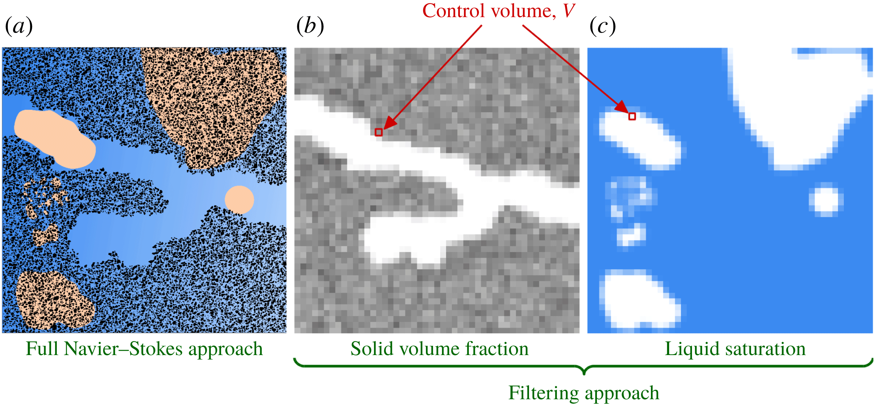
Schematic of the micro-continuum approach extended to multiple fluid phases. (a) The full Navier–Stokes representation of the physics (solid grains in black, liquid in blue and gas in orange); (b) map of the solid volume fraction after filtering; (c) map of the liquid saturation after filtering.

Numerical simulation of multiphase dissolution at the pore scale is challenging because it involves multiple interfaces (gas/liquid, fluid/solid) that evolve as a function of the details of the reactive transport. Instead of the full Navier–Stokes simulation approach (see figure 1
a), we employ a micro-continuum formulation. That is, all the information regarding the solid structure at a scale smaller than the computational cells (control volumes) is filtered and modelled as a fluid/solid aggregate. In the DBS approach, all the physical variables of the solid–fluids system are averaged over the cell’s control volume,
 $V$
. Cells that contain pore space (fluids) and those that contain solid are differentiated using the scalar field
 $\unicode[STIX]{x1D700}$
, which corresponds to the volume fraction of the pore space in the control volumes. It is a field with different values in the computational domain that range from 0 to 1. This filtering approach is illustrated in figure 1(b). The free zone is characterized by
 $\unicode[STIX]{x1D700}=1$
, and the flow is governed by the two-phase Navier–Stokes equations. For intermediate values,
 $0<\unicode[STIX]{x1D700}<1$
, there are solid ‘obstacles’ in the control volume, and the physics of flow and transport in porous media is applied. When
 $\unicode[STIX]{x1D700}=0$
, the control volume contains solid only, and there is no flow. We assume that the cells that are fully occupied by the solid always contain a tiny porosity,
 $\unicode[STIX]{x1D700}=0\equiv 0.001$
, and that allows for a single-field DBS formulation regardless of the make-up of a computational cell. Different from other micro-continuum models proposed to simulate core-scale phenomena (Liu et al.
Reference Liu, Ormond, Bartko, Ying and Ortoleva1997; Ormond & Ortoleva Reference Ormond and Ortoleva2000; Golfier et al.
Reference Golfier, Zarcone, Bazin, Lenormand, Lasseux and Quintard2002; Scheibe et al.
Reference Scheibe, Perkins, Richmond, McKinley, Romero-Gomez, Oostrom, Wietsma, Serkowski and Zachara2015; Soulaine & Tchelepi Reference Soulaine and Tchelepi2016a
), this work uses a DBS formulation to simulate pore-scale physics. Thus, only the bounding values
 $\unicode[STIX]{x1D700}=1$
and
 $\unicode[STIX]{x1D700}=0$
are used to map the entire structure at the pore scale. The intermediate values of the pore space (or the solid) describe the interface between the fluid and the solid. This approach has been used successfully to track the displacement of a fluid/solid interface during dissolution in the presence of a single-phase fluid (Soulaine et al.
Reference Soulaine, Roman, Kovscek and Tchelepi2017).
The micro-continuum approach is a physically based model, whereby the governing equations are locally averaged. This approach inherits all the theoretical developments of the physics of flow and transport in porous media using the method of volume averaging (Whitaker Reference Whitaker1999). The micro-continuum approach relies on the fact that for each variable of the system, a single conservation equation holds for both the porous and pore (fluids) domains: in the free zone (pore space), the equations tend asymptotically to the standard equations of fluid dynamics, while in the porous regions they reduce to the partial differential equations that govern flow and transport in porous media. For example, for single phase flow, the Darcy–Brinkman–Stokes (DBS) equation (Brinkman Reference Brinkman1947) can be used to simulate flow in a channel surrounded by a porous matrix (Neale & Nader Reference Neale and Nader1974; Soulaine et al. Reference Soulaine, Gjetvaj, Garing, Roman, Russian, Gouze and Tchelepi2016; Soulaine & Tchelepi Reference Soulaine and Tchelepi2016a ). In the channel, the drag force vanishes since there is no solid, and the DBS formalism turns to the Stokes equation. In the ‘porous’ matrix, the drag force is dominant with respect to the viscous term, and the momentum balance tends toward Darcy’s law. In this work, the solid phase is described by a low-permeability low-porosity matrix and the Darcy term is used to penalize the flow in this region.
When dissolution occurs in a control volume, the volume fraction of solid,
 $\unicode[STIX]{x1D700}_{s}$
, decreases. Consequently, the local porosity,
 $\unicode[STIX]{x1D700}$
, increases. This is because the relation
 $$\begin{eqnarray}\displaystyle \unicode[STIX]{x1D700}_{s}=1-\unicode[STIX]{x1D700} & & \displaystyle\end{eqnarray}$$
is always valid. The variation of the solid volume fraction is used to track the evolution of the pore topology.
In the micro-continuum approach extended to multiphase system, the pore space is occupied by two fluids, namely gas and liquid denoted
 $g$
and
 $l$
, respectively. The distribution of fluids in the domain is described by the volume fraction of gas,
 $\unicode[STIX]{x1D700}_{g}$
, and the volume fraction of liquid,
 $\unicode[STIX]{x1D700}_{l}$
, in every control volumes (see figure 1
c). Note that by construction, the relations
 $\unicode[STIX]{x1D700}_{s}+\unicode[STIX]{x1D700}_{g}+\unicode[STIX]{x1D700}_{l}=1$
and
 $\unicode[STIX]{x1D700}=\unicode[STIX]{x1D700}_{g}+\unicode[STIX]{x1D700}_{l}$
are always valid. These quantities evolve with chemical reactions at the mineral surface and with the hydrodynamics of the system. The distribution of the fluids in the domain is tracked using the concept of saturation,
 $S_{f}$
with
 $f=l,g$
, that represents the ratio of the volume occupied by the
 $f$
-phase over the volume of the pore space,
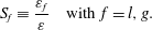 $$\begin{eqnarray}\displaystyle S_{f}\equiv \frac{\unicode[STIX]{x1D700}_{f}}{\unicode[STIX]{x1D700}}\quad \text{with}~f=l,g. & & \displaystyle\end{eqnarray}$$
It has the advantage to be normalized:
 $S_{f}$
varies in the range 0–1. The relation,
 $$\begin{eqnarray}\displaystyle S_{l}+S_{g}=1, & & \displaystyle\end{eqnarray}$$
is always satisfied. Thus, we only need to compute the liquid (or gas) saturation. In the pore space, i.e.
 $\unicode[STIX]{x1D700}=1$
, saturation is similar to the colour function used in the volume-of-fluid (VOF) approach to track fluid/fluid interfaces. Namely, in the control volumes occupied by liquid only,
 $S_{l}=1$
; in regions occupied by gas only,
 $S_{l}=0$
; and for gas/liquid interface,
 $0<S_{l}<1$
.
As for the volume fractions and the saturation, all the physical variables of the system can be defined as averaged quantities over the control volume. For each phase (
 $f=l,g$
), we define the phase averaged pressure
 $\bar{p}_{f}=1/V_{f}\int _{V_{f}}p_{f}\,\text{d}V$
, the phase averaged velocity
 $\bar{\mathsf{v}}_{f}=1/V_{f}\int _{V_{f}}\mathsf{v}_{f}\,\text{d}V$
and the phase averaged mass fraction of a chemical species
 $A$
in the mixture,
 $\bar{\unicode[STIX]{x1D714}}_{f,A}=1/V_{f}\int _{V_{f}}\unicode[STIX]{x1D714}_{f,A}\,\text{d}V$
where
 $V_{f}$
is the volume occupied by the fluid
 $f=l,g$
in the control volume.
In the pore-scale multiphase micro-continuum model, the problem is formulated in terms of single field (global variables) regardless of the content of cell. Hence, a single momentum equation is used to solve for the mixture velocity,
 $\bar{\mathsf{v}}$
, defined as,
 $$\begin{eqnarray}\displaystyle \bar{\mathsf{v}}=\unicode[STIX]{x1D700}_{l}\bar{\mathsf{v}}_{l}+\unicode[STIX]{x1D700}_{g}\bar{\mathsf{v}}_{g}=\unicode[STIX]{x1D700}(S_{l}\bar{\mathsf{v}}_{l}+(1-S_{l})\bar{\mathsf{v}}_{g}). & & \displaystyle\end{eqnarray}$$
On the one hand, in the free zone,
 $\bar{\mathsf{v}}$
corresponds to the velocity field used in the VOF method: if
 $S_{l}=1$
, it denotes the velocity of the liquid, if
 $S_{l}=0$
, it depicts the velocity of the gas phase and if
 $0<S_{l}<1$
, it corresponds to the velocity of the gas/liquid interface. In the solid–fluids aggregates domain,
 $\bar{\mathsf{v}}$
corresponds to Darcy’s mixture velocity (Wang & Beckermann Reference Wang and Beckermann1993).
The single-field pressure is defined as
 $$\begin{eqnarray}\displaystyle \bar{p}=S_{l}\bar{p}_{l}+(1-S_{l})\bar{p}_{g}, & & \displaystyle\end{eqnarray}$$
and the concentration field for species
 $A$
as,
 $$\begin{eqnarray}\displaystyle \bar{\unicode[STIX]{x1D714}}_{A}=S_{l}\bar{\unicode[STIX]{x1D714}}_{l,A}+(1-S_{l})\bar{\unicode[STIX]{x1D714}}_{g,A}. & & \displaystyle\end{eqnarray}$$
Next, we introduce the governing equations for the evolution of the solid volume fraction
 $\unicode[STIX]{x1D700}_{s}$
, the saturation
 $S_{l}$
, the velocity field
 $\bar{\mathsf{v}}$
, the pressure
 $\bar{p}$
and the concentration field
 $\bar{\unicode[STIX]{x1D714}}_{A}$
.
2.2 Mass transfer
In this system, the pore geometry, and hence the porosity, permeability and flow behaviour evolve with the chemical reactions that take place at the solid boundaries. For acidization processes involving hydrochloric acid (HCl) in carbonate formations, mineral dissolution is dictated by the following reactions at the surface of the calcite crystal:
 $$\begin{eqnarray}\displaystyle & \displaystyle \text{CaCO}_{3(s)}+2\text{HCl}_{(aq)}\rightarrow \text{CaCl}_{2(aq)}+\text{CO}_{2(aq)}+\text{H}_{2}\text{O}_{(l)} & \displaystyle\end{eqnarray}$$
 $$\begin{eqnarray}\displaystyle & \displaystyle \text{CO}_{2(aq)}\rightarrow \text{CO}_{2(g)}. & \displaystyle\end{eqnarray}$$
The
 $\text{CO}_{2}$
forms in the aqueous phase and then nucleates as a gas phase on the surface of the grain. We neglect the
 $\text{CO}_{2(aq)}$
in the mass balance and we consider that the
 $\text{CO}_{2}$
from the aqueous phase instantaneously goes to the gas phase. Moreover, we assume that the characteristic time of the
 $\text{CO}_{2}$
mass transfer from the gas to the liquid phase is much longer compared with the rate of
 $\text{CO}_{2}$
production from the dissolution of the rock. Hence, HCl is the only species that needs to be tracked to compute the reaction rate at the solid surface,
 ${\dot{m}}_{l,HCl}$
. Then, it follows that the rates of the phase change for the solid, gas and liquid phases are directly described by the reaction rate of the acid (HCl). Consequently, we can write:
 $$\begin{eqnarray}\displaystyle \dot{m_{i}}=\unicode[STIX]{x1D6FE}_{i}{\dot{m}}_{l,HCl}\quad \text{with}~i=s,l,g, & & \displaystyle\end{eqnarray}$$
where
 $\unicode[STIX]{x1D6FE}_{i}$
is based on molar mass and stoichiometric coefficients:
 $\unicode[STIX]{x1D6FE}_{s}=M_{CaCO_{3}}/2M_{HCl}$
,
 $\unicode[STIX]{x1D6FE}_{g}=-M_{CO_{2}}/2M_{HCl}$
and
 $\unicode[STIX]{x1D6FE}_{l}=(2M_{HCl}-M_{CaCl_{2}}-M_{H_{2}O})/2M_{HCl}$
.
2.3 Mass balance equation
The volume fractions of the three phases (solid, liquid, gas) that occupy the domain evolve in time as a function of the hydrodynamics and the chemical reactions at the solid surface. The volume fraction of solid in a control volume is an unknown (degree-of-freedom) of the system, and its evolution is governed by the mass balance equation:
 $$\begin{eqnarray}\displaystyle \frac{\unicode[STIX]{x2202}\unicode[STIX]{x1D700}_{s}\unicode[STIX]{x1D70C}_{s}}{\unicode[STIX]{x2202}t}={\dot{m}}_{s}, & & \displaystyle\end{eqnarray}$$
where
 $\unicode[STIX]{x1D70C}_{s}$
is the density of the solid, and
 ${\dot{m}}_{s}$
, is the rate of dissolution of solid into gas and liquid. The latter has a non-zero value only at the fluid/solid interface. The dissolved mass goes into the two fluid phases. Hence, the conservation laws for the liquid and gas are:
 $$\begin{eqnarray}\displaystyle \frac{\unicode[STIX]{x2202}\unicode[STIX]{x1D700}_{l}\unicode[STIX]{x1D70C}_{l}}{\unicode[STIX]{x2202}t}+\unicode[STIX]{x1D735}\boldsymbol{\cdot }(\unicode[STIX]{x1D700}_{l}\unicode[STIX]{x1D70C}_{l}\bar{\mathsf{v}}_{l})=\dot{m_{l}}, & & \displaystyle\end{eqnarray}$$
and,
 $$\begin{eqnarray}\displaystyle \frac{\unicode[STIX]{x2202}\unicode[STIX]{x1D700}_{g}\unicode[STIX]{x1D70C}_{g}}{\unicode[STIX]{x2202}t}+\unicode[STIX]{x1D735}\boldsymbol{\cdot }(\unicode[STIX]{x1D700}_{g}\unicode[STIX]{x1D70C}_{g}\bar{\mathsf{v}}_{g})={\dot{m}}_{g}, & & \displaystyle\end{eqnarray}$$
where
 $\unicode[STIX]{x1D70C}_{l}$
and
 $\unicode[STIX]{x1D70C}_{g}$
stand for the density of the liquid and gas, respectively. The source terms
 $\dot{m_{l}}$
and
 $\dot{m_{g}}$
denote the rate of production of liquid and gas, respectively.
In our DBS framework, we recast this set of equations into a global mass balance equation and a saturation (transport) equation. The global mass conservation equation is obtained by summing (2.10)–(2.12). Assuming that both the liquid and the gas phases are incompressible, we have
 $$\begin{eqnarray}\displaystyle \unicode[STIX]{x1D735}\boldsymbol{\cdot }\bar{\mathsf{v}}={\dot{m}}_{l,HCl}\left(\frac{\unicode[STIX]{x1D6FE}_{l}}{\unicode[STIX]{x1D70C}_{l}}+\frac{\unicode[STIX]{x1D6FE}_{g}}{\unicode[STIX]{x1D70C}_{g}}+\frac{\unicode[STIX]{x1D6FE}_{s}}{\unicode[STIX]{x1D70C}_{s}}\right). & & \displaystyle\end{eqnarray}$$
To track the liquid saturation, the mass conservation equation for the liquid, equation (2.11) is transformed into (see appendix A for the derivation)
 $$\begin{eqnarray}\displaystyle \frac{\unicode[STIX]{x2202}\unicode[STIX]{x1D700}S_{l}}{\unicode[STIX]{x2202}t}+\unicode[STIX]{x1D735}\boldsymbol{\cdot }(\bar{\mathsf{v}}S_{l})+\unicode[STIX]{x1D735}\boldsymbol{\cdot }(\unicode[STIX]{x1D700}S_{l}(1-S_{l})\bar{\mathsf{v}}_{r})=\frac{\dot{m_{l}}}{\unicode[STIX]{x1D70C}_{l}}, & & \displaystyle\end{eqnarray}$$
where
 $\bar{\mathsf{v}}_{r}=(\bar{\mathsf{v}}_{l}-\bar{\mathsf{v}}_{g})$
is a compression velocity. In the free zone,
 $\unicode[STIX]{x1D700}=1$
, and this equation turns into the phase indicator equation used in the algebraic VOF solver implemented in OpenFOAM® (Rusche Reference Rusche2003). The last term on the left-hand side is non-zero only in the gas/liquid transition region. It is used to sharpen the interface. The value of the relative velocity,
 $\bar{\mathsf{v}}_{r}$
, is estimated from the maximum velocity magnitude in this interfacial area (Rusche Reference Rusche2003).
2.4 Momentum balance equation and adhesion to the solid
The flow problem under consideration involves the evolution of multiple interfaces. The delineation between the free zone, i.e.
 $\unicode[STIX]{x1D700}=1$
, and the solid (modelled as a porous medium) changes as the solid dissolves. Thus, the topology of the void space changes substantially. In the free zone, the gas and liquid evolve as two immiscible fluids separated by an interface with surface tension. When the three phases meet, the fluid/fluid interface forms a contact angle with the solid surface, which depends on the wettability and the hydrodynamic conditions.
To model the momentum balance equation, we adopt a combination of the Darcy–Brinkman–Stokes equation, which has proven to be quite effective for solving single-phase dissolution problems (Soulaine et al. Reference Soulaine, Roman, Kovscek and Tchelepi2017), and the classic VOF method used to track gas–liquid interfaces on a fixed Eulerian grid (Hirt & Nichols Reference Hirt and Nichols1981). In this model, a single equation holds for the liquid, gas and the porous region. The momentum equation is expressed as:
 $$\begin{eqnarray}\displaystyle \frac{\unicode[STIX]{x1D70C}}{\unicode[STIX]{x1D700}}\left(\frac{\unicode[STIX]{x2202}\bar{\mathsf{v}}}{\unicode[STIX]{x2202}t}+\frac{\bar{\mathsf{v}}}{\unicode[STIX]{x1D700}}\boldsymbol{\cdot }\unicode[STIX]{x1D735}\bar{\mathsf{v}}\right)=-\unicode[STIX]{x1D735}\bar{p}+\unicode[STIX]{x1D735}\boldsymbol{\cdot }\left(\frac{\unicode[STIX]{x1D707}}{\unicode[STIX]{x1D700}}(\unicode[STIX]{x1D735}\bar{\mathsf{v}}+^{t}\unicode[STIX]{x1D735}\bar{\mathsf{v}})\right)+\boldsymbol{F}_{c}-\unicode[STIX]{x1D707}k^{-1}\bar{\mathsf{v}}, & & \displaystyle\end{eqnarray}$$
where
 $\unicode[STIX]{x1D70C}$
is the density,
 $\unicode[STIX]{x1D707}$
is the dynamic viscosity,
 $\boldsymbol{F}_{c}$
is the surface-tension force due to curvature of the interface. The last term of the right-hand side,
 $\unicode[STIX]{x1D707}k^{-1}\bar{\mathsf{v}}$
, represents the momentum exchange term between the fluids and the solid phase. The density and viscosity depend on the saturation through the relations,
 $\unicode[STIX]{x1D70C}=\unicode[STIX]{x1D70C}_{l}S_{l}+\unicode[STIX]{x1D70C}_{g}(1-S_{l})$
and
 $\unicode[STIX]{x1D707}=\unicode[STIX]{x1D707}_{l}S_{l}+\unicode[STIX]{x1D707}_{g}(1-S_{l})$
. This model is similar to the penalization technique applied to the VOF method proposed by Horgue, Prat & Quintard (Reference Horgue, Prat and Quintard2014). Here, there is the additional complexity that the solid structure evolves in time. Horgue et al. (Reference Horgue, Prat and Quintard2014) solve a momentum equation similar to (2.15) and use the flow resistance term,
 $\unicode[STIX]{x1D707}k^{-1}\bar{\mathsf{v}}$
, to force the velocity values to near zero in regions identified as solid, and therefore enforce a no-slip boundary condition at the immersed boundaries. The wall adhesion condition is ensured by local modification of the surface tension force,
 $\boldsymbol{F}_{c}$
, at the wall boundary to enforce the value of the contact angle formed by the gas–liquid interface and the solid surface.
As for the Darcy–Brinkman–Stokes model applied to the simulation of flow in large channels surrounded by porous media (Neale & Nader Reference Neale and Nader1974), the resistance term,
 $\unicode[STIX]{x1D707}k^{-1}\bar{\mathsf{v}}$
, vanishes in the free zone (
 $\unicode[STIX]{x1D700}=1$
), so that (2.15) reduces to the classic VOF momentum equation, and is dominant in the porous regions so that the momentum equation tends toward Darcy’s law in these regions. Because the fluids/solid interface moves with the dissolution process, the value of the local permeability evolves with the local porosity,
 $\unicode[STIX]{x1D700}$
.
We use a Kozeny–Carman relationship to compute
 $k$
from the local porosity (Voller Reference Voller2009):
 $$\begin{eqnarray}\displaystyle k^{-1}=k_{0}^{-1}\frac{(1-\unicode[STIX]{x1D700})^{2}}{\unicode[STIX]{x1D700}^{3}}, & & \displaystyle\end{eqnarray}$$
with
 $\sqrt{k_{0}}$
the characteristic length of the micro-structure. With this formulation,
 $k^{-1}=0~\text{m}^{-2}$
in the free zone and tends towards a very large value when the porosity is close to zero. In the latter case, the velocity in the porous region drops down to values near zero, which mimics a solid with no flow as in the fictitious domain approach (Angot, Bruneau & Fabrie Reference Angot, Bruneau and Fabrie1999; Khadra et al.
Reference Khadra, Angot, Parneix and Caltagirone2000; Horgue et al.
Reference Horgue, Prat and Quintard2014; Soulaine & Tchelepi Reference Soulaine and Tchelepi2016a
). With dissolution, the cell porosity evolves and that changes the local permeability until all the solid contained in a computational cell is fully consumed, and the model switches automatically from Darcy’s law to the VOF-based Navier–Stokes representation.
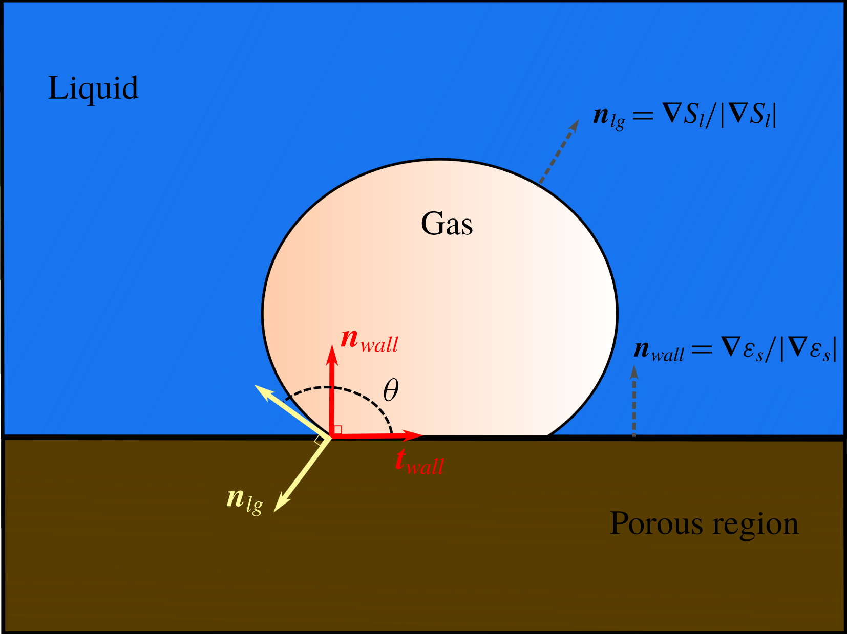
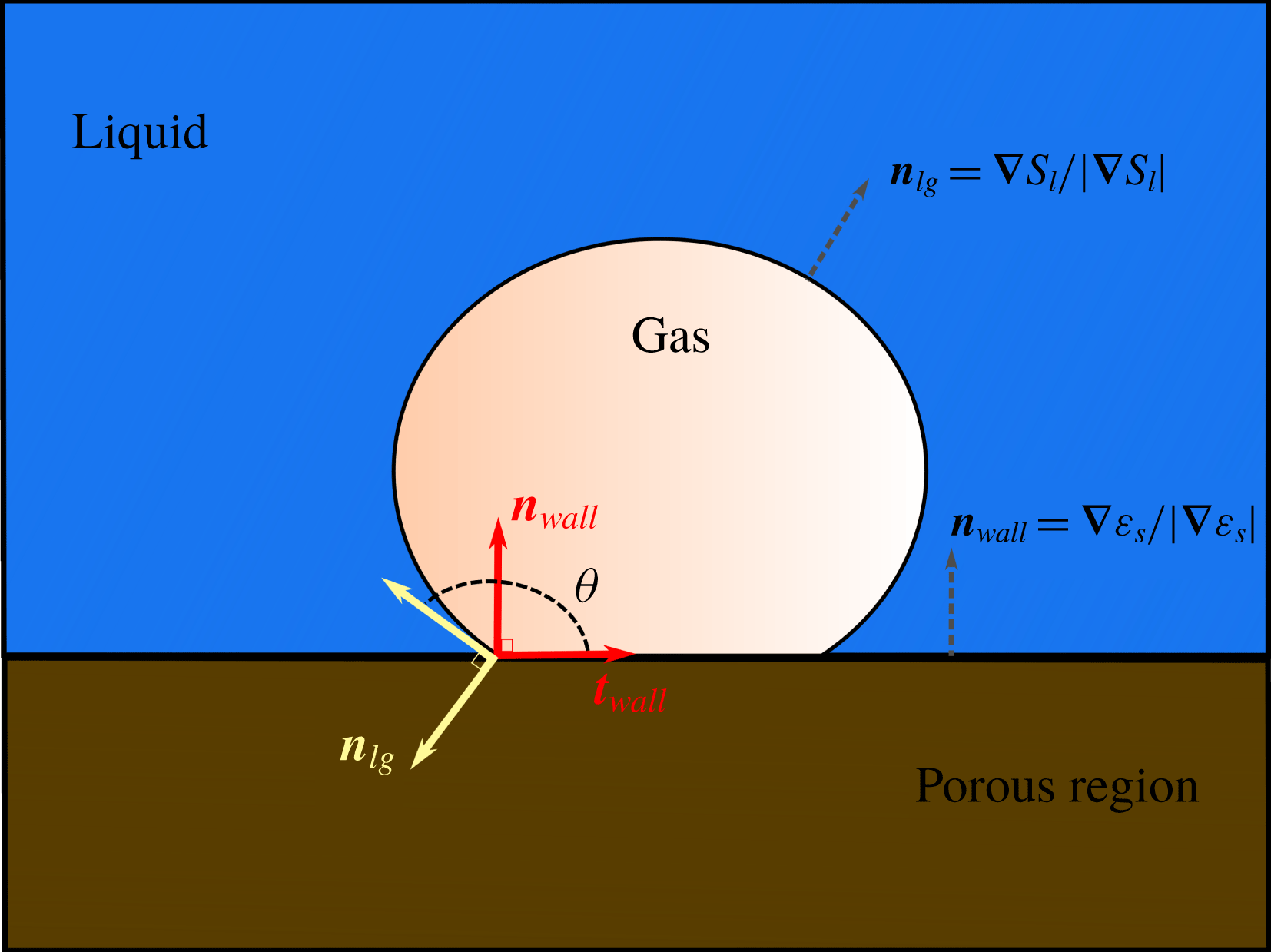
Illustration of the wall adhesion condition. The normal to the gas/liquid interface,
 $\boldsymbol{n}_{lg}$
, forms an angle
 $\unicode[STIX]{x1D703}$
with the normal to the solid wall,
 $\boldsymbol{n}_{wall}$
. These two normal vectors are computed from the gradient of the volume fraction fields.
The capillary effects due to the surface tension between the two fluids and the wettability with respect to the solid minerals are described by a unique volumetric source term,
 $\boldsymbol{F}_{c}$
, defined throughout the computational grid. The nature of this term, however, is different according to the cell porosity. In the free zone, the two fluid phases are immiscible, and the curvature of the interface leads to a discontinuity in the stress to balance the pressure gradient according to Young–Laplace law. At the fluid/solid boundary, the liquid–gas interface meets the solid surface forming a contact angle that reflects the wettability of the system. To model
 $\boldsymbol{F}_{c}$
with a unique formulation that is valid everywhere in the computational domain, we adopt the strategy proposed by Horgue et al. (Reference Horgue, Prat and Quintard2014). Regardless of the region of interest, we have
 $$\begin{eqnarray}\displaystyle \boldsymbol{F}_{c}=\unicode[STIX]{x1D700}\unicode[STIX]{x1D70E}\unicode[STIX]{x1D735}\boldsymbol{\cdot }(\hat{\boldsymbol{n}}_{lg})\unicode[STIX]{x1D735}S_{l}, & & \displaystyle\end{eqnarray}$$
where
 $\unicode[STIX]{x1D70E}$
is the surface tension between the gas and the liquid, and
 $\hat{\boldsymbol{n}}_{lg}$
is the normal to the gas/liquid interface locally modified to account for the wall adhesion condition. In the clear-fluid region,
 $\hat{\boldsymbol{n}}_{lg}$
corresponds to the normal to the gas–liquid interface
 $\boldsymbol{n}_{lg}=\unicode[STIX]{x1D735}S_{l}/\Vert \unicode[STIX]{x1D735}S_{l}\Vert$
and we have
 $\boldsymbol{F}_{c}=\unicode[STIX]{x1D70E}\unicode[STIX]{x1D735}\boldsymbol{\cdot }(\unicode[STIX]{x1D735}S_{l}/\Vert \unicode[STIX]{x1D735}S_{l}\Vert )\unicode[STIX]{x1D735}S_{l}$
, which corresponds to the continuum surface force (CSF) introduced by Brackbill, Kothe & Zemach (Reference Brackbill, Kothe and Zemach1992). At the solid boundaries,
 $\hat{\boldsymbol{n}}_{lg}$
is modified to enforce the wall adhesion condition:
 $$\begin{eqnarray}\displaystyle \hat{\boldsymbol{n}}_{lg}=\cos \unicode[STIX]{x1D703}\boldsymbol{n}_{wall}+\sin \unicode[STIX]{x1D703}\boldsymbol{t}_{wall}, & & \displaystyle\end{eqnarray}$$
where
 $\boldsymbol{n}_{wall}$
and
 $\boldsymbol{t}_{wall}$
are the normal and tangent vectors to the solid surface, respectively, and
 $\unicode[STIX]{x1D703}$
is the contact angle (see figure 2).
We use the correction strategy proposed by Horgue et al. (Reference Horgue, Prat and Quintard2014): after solving the saturation equation. The normal,
 $\boldsymbol{n}_{lg}$
, to the gas/liquid interface does not satisfy (2.18) but forms an angle
 $\unicode[STIX]{x1D703}_{I}$
with the vector normal to the wall,
 $\boldsymbol{n}_{wall}$
. That is,
 $\unicode[STIX]{x1D703}_{I}=\cos ^{-1}(\boldsymbol{n}_{wall}\boldsymbol{\cdot }\boldsymbol{n}_{lg})$
. The locally modified normal vector,
 $\hat{\boldsymbol{n}}_{lg}$
, used to compute the capillary forces in (2.17) – and defined over the entire computational domain – is corrected to enforce the correct value of
 $\unicode[STIX]{x1D703}$
by using the formula:
 $$\begin{eqnarray}\displaystyle \hat{\boldsymbol{n}}_{lg}=\frac{\cos \unicode[STIX]{x1D703}-\cos \unicode[STIX]{x1D703}_{I}\cos (\unicode[STIX]{x1D703}_{I}-\unicode[STIX]{x1D703})}{1-\cos ^{2}\unicode[STIX]{x1D703}_{I}}\boldsymbol{n}_{wall}+\frac{\cos (\unicode[STIX]{x1D703}_{I}-\unicode[STIX]{x1D703})-\cos \unicode[STIX]{x1D703}_{I}\cos \unicode[STIX]{x1D703}}{1-\cos ^{2}\unicode[STIX]{x1D703}_{I}}\boldsymbol{n}_{lg}. & & \displaystyle\end{eqnarray}$$
The derivation of this formula can be found in appendix B. The normal vectors to the solid wall and to the gas/liquid interface are computed using the volume fractions of the solid and liquid, respectively, with
 $\boldsymbol{n}_{wall}=\unicode[STIX]{x1D735}\unicode[STIX]{x1D700}_{s}/\Vert \unicode[STIX]{x1D735}\unicode[STIX]{x1D700}_{s}\Vert$
and
 $\boldsymbol{n}_{lg}=\unicode[STIX]{x1D735}S_{l}/\Vert \unicode[STIX]{x1D735}S_{l}\Vert$
. With (2.19), both Brackbill’s CSF and the wall adhesion condition are satisfied using a unique formulation. In the free region,
 $\boldsymbol{n}_{wall}=\mathbf{0}$
and we have
 $\hat{\boldsymbol{n}}_{lg}/\Vert \hat{\boldsymbol{n}}_{lg}\Vert =\boldsymbol{n}_{lg}/\Vert \boldsymbol{n}_{lg}\Vert$
, and then
 $\boldsymbol{F}_{c}=\unicode[STIX]{x1D70E}\unicode[STIX]{x1D735}\boldsymbol{\cdot }(\unicode[STIX]{x1D735}S_{l}/\Vert \unicode[STIX]{x1D735}S_{l}\Vert )\unicode[STIX]{x1D735}S_{l}$
. At the solid boundary, equation (2.19) automatically enforces the wall adhesion condition,
 $\hat{\boldsymbol{n}}_{lg}=\cos \unicode[STIX]{x1D703}\boldsymbol{n}_{wall}+\sin \unicode[STIX]{x1D703}\boldsymbol{t}_{wall}$
. Refer to Horgue et al. (Reference Horgue, Prat and Quintard2014) for details regarding the implementation and validation of this technique. In the porous regions, the surface-tension forces under confinement corresponds to the gradient of the capillary pressure,
 $\boldsymbol{F}_{c}=\unicode[STIX]{x1D735}p_{c}=(\unicode[STIX]{x2202}p_{c}/\unicode[STIX]{x2202}S_{l})\unicode[STIX]{x1D735}S_{l}$
. In the pore-scale simulations presented in this paper, the porous regions are initially saturated by the liquid at the thermodynamic equilibrium with the solid. Hence, there is no chemical reaction except at the boundaries of the porous regions. Therefore, in the matrix, we always have
 $\unicode[STIX]{x1D735}S_{l}=\mathbf{0}$
, and then
 $\boldsymbol{F}_{c}=\mathbf{0}$
.
2.5 Concentration equation
In a multiphase system, the chemical components are present in both fluid phases. For instance, there is
 $\text{CO}_{2}$
in the gas phase and dissolved
 $\text{CO}_{2}$
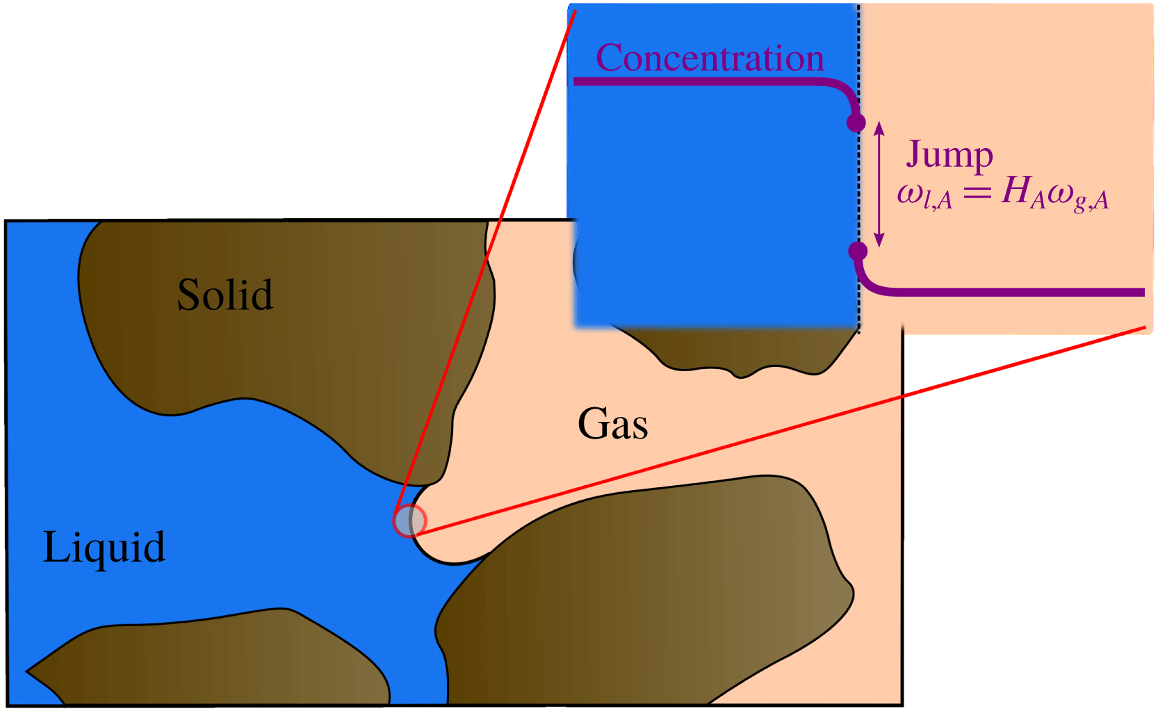
in the aqueous phase. The component concentration in each phase is governed by the advection–diffusion conservation equations coupled with the thermodynamic equilibrium condition at the gas/liquid interface. This latter condition is usually described using a partitioning relation, such as Henry’s laws (see figure 3):
 $$\begin{eqnarray}\displaystyle \unicode[STIX]{x1D714}_{l,A}=H_{A}\unicode[STIX]{x1D714}_{g,A}, & & \displaystyle\end{eqnarray}$$
where
 $H_{A}$
is the partitioning coefficient or Henry’s constant. When this condition is not fulfilled, there is a mass transfer from one phase to one another in order to reach thermodynamic equilibrium.
Illustration of the mass transfer between two immiscible phases. If Henry’s law is not satisfied at the gas/liquid interface, then there is a mass transfer across the interface in order to reach thermodynamic equilibrium.

In the micro-continuum approach, a single conservation equation governs the global concentration field,
 $\bar{\unicode[STIX]{x1D714}}_{A}$
. Two challenges arise to transport
 $\bar{\unicode[STIX]{x1D714}}_{A}$
using a single equation in a domain that contains two fluids. In the free zone, this equation has to be compatible with the VOF formulation to transport the species in a two-fluid system, where the thermodynamic equilibrium condition at the interface between the fluids, equation (2.20), is always satisfied. This equation should also capture the chemical reaction at the minerals surface. The model we propose for the evolution of
 $\bar{\unicode[STIX]{x1D714}}_{A}$
is a combination of the method proposed by Haroun, Legendre & Raynal (Reference Haroun, Legendre and Raynal2010) to transport a concentration field in a two-fluid system and the immersed boundary technique for micro-continuum models proposed by Soulaine et al. (Reference Soulaine, Roman, Kovscek and Tchelepi2017). Specifically, we write
 $$\begin{eqnarray}\displaystyle \frac{\unicode[STIX]{x2202}\unicode[STIX]{x1D700}\unicode[STIX]{x1D70C}\bar{\unicode[STIX]{x1D714}}_{A}}{\unicode[STIX]{x2202}t}+\unicode[STIX]{x1D735}\boldsymbol{\cdot }(\unicode[STIX]{x1D70C}\bar{\mathsf{v}}\bar{\unicode[STIX]{x1D714}}_{A})=\unicode[STIX]{x1D735}\boldsymbol{\cdot }(\unicode[STIX]{x1D700}\unicode[STIX]{x1D70C}D_{A}^{\ast }(\unicode[STIX]{x1D735}\bar{\unicode[STIX]{x1D714}}_{A}+\unicode[STIX]{x1D731}_{A}))-{\dot{m}}_{l,A}, & & \displaystyle\end{eqnarray}$$
where
 $D_{A}^{\ast }$
is the effective diffusion coefficient,
 $\unicode[STIX]{x1D731}_{A}$
is the continuum species transfer (CST) flux (Haroun et al.
Reference Haroun, Legendre and Raynal2010; Marschall et al.
Reference Marschall, Hinterberger, Schüler, Habla and Hinrichsen2012; Graveleau et al.
Reference Graveleau, Soulaine and Tchelepi2017; Maes & Geiger Reference Maes and Geiger2017; Maes & Soulaine Reference Maes and Soulaine2018) and
 ${\dot{m}}_{l,A}$
is a reaction rate at the mineral surface. This equation is valid everywhere in the computational domain, regardless the cells content.
The effective diffusion coefficient,
 $D_{A}^{\ast }$
, is:
 $$\begin{eqnarray}\displaystyle \unicode[STIX]{x1D700}D_{A}^{\ast }=\unicode[STIX]{x1D700}^{2}\frac{D_{l,A}D_{g,A}}{S_{l}D_{g,A}+(1-S_{l})D_{l,A}}, & & \displaystyle\end{eqnarray}$$
where
 $D_{g,A}$
and
 $D_{l,A}$
are the molecular diffusivity of the component
 $A$
in the gas and liquid phase, respectively. Haroun et al. (Reference Haroun, Legendre and Raynal2010) and Deising, Marschall & Bothe (Reference Deising, Marschall and Bothe2016) have demonstrated that this harmonic formulation is more robust than a simple mixing rule. In the free zone,
 $D_{A}^{\ast }=D_{g,A}$
in the gas phase and
 $D_{A}^{\ast }=D_{l,A}$
in the liquid phase. Similar to the single-phase micro-continuum model of Soulaine et al. (Reference Soulaine, Roman, Kovscek and Tchelepi2017), the exponent 2 allows the value of diffusion in the solid regions to drop to near zero.
The additional flux in (2.21),
 $\unicode[STIX]{x1D731}_{A}$
, describes the thermodynamic equilibrium at the gas/liquid interface. It transforms the solubility condition, equation (2.20), into a volumetric term under the framework of the VOF formulation (Haroun et al.
Reference Haroun, Legendre and Raynal2010). We have:
 $$\begin{eqnarray}\displaystyle \unicode[STIX]{x1D731}_{A}=\frac{\bar{\unicode[STIX]{x1D714}}_{A}(\unicode[STIX]{x1D70C}_{g}H_{A}-\unicode[STIX]{x1D70C}_{l})}{\unicode[STIX]{x1D70C}_{l}H_{A}S_{l}+\unicode[STIX]{x1D70C}_{g}(1-S_{l})}\unicode[STIX]{x1D735}S_{l}. & & \displaystyle\end{eqnarray}$$
The CST term is responsible for the concentration jump at the interface, while the flux continuity across the interface is always insured. This approach is similar of the continuum surface force (CSF) used for the modelling of the surface tension between two fluids (Brackbill et al. Reference Brackbill, Kothe and Zemach1992).
The reaction term,
 ${\dot{m}}_{l,A}$
, describes the chemical reaction of the mineral surface and the acid species included in the liquid phase. In (2.21), this term is negative because acid concentration decreases at the liquid/solid interface due to the chemical reaction. For a first-order reaction rate, we have
 $$\begin{eqnarray}\displaystyle {\dot{m}}_{l,A}=\unicode[STIX]{x1D70C}_{l}a_{v}^{l}r\bar{\unicode[STIX]{x1D714}}_{A}, & & \displaystyle\end{eqnarray}$$
where
 $r$
is the constant of reaction and
 $a_{v}^{l}$
is the wetted effective surface area in one grid block. The latter is a function of the specific area,
 $a_{v}$
and the liquid saturation. In the micro-continuum formulation for pore-scale simulation with a sharp interface between the non-obstructed regions and the low-permeability low-porosity regions, the surface area per control volume can be evaluated using the porosity gradient,
 $a_{v}=\Vert \unicode[STIX]{x1D735}\unicode[STIX]{x1D700}\Vert$
(Soulaine et al.
Reference Soulaine, Roman, Kovscek and Tchelepi2017). To enforce the reactive boundary solution at the fluid/solid interface only, the specific area is computed as
 $a_{v}=\Vert \unicode[STIX]{x1D735}\unicode[STIX]{x1D700}\Vert \unicode[STIX]{x1D713}$
, where
 $\unicode[STIX]{x1D713}$
is a diffuse interface function. We use
 $\unicode[STIX]{x1D713}=4\unicode[STIX]{x1D700}(1-\unicode[STIX]{x1D700})$
(Luo et al.
Reference Luo, Quintard, Debenest and Laouafa2012). Moreover, because the reaction occurs on wetted surface only, we simply write
 $a_{v}^{l}=a_{v}S_{l}$
.
2.6 Numerical implementation
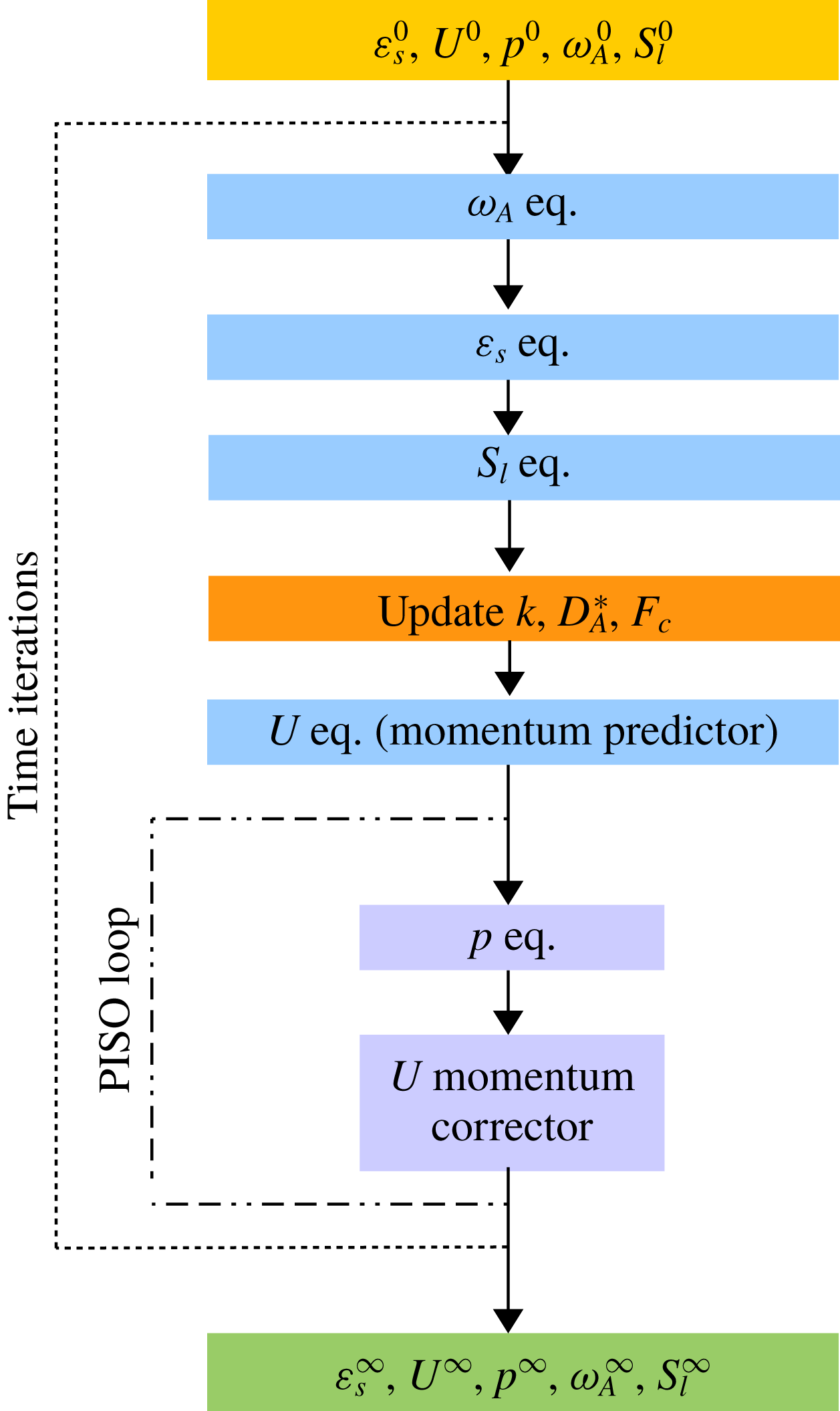
The mathematical model formed by (2.13)–(2.15) and (2.21) has been implemented in the open-source computational fluid dynamics platform OpenFOAM® (http://www.openfoam.org). The equations are first discretized using a finite-volume method and solved sequentially. The pressure–velocity coupling is handled by a predictor–corrector strategy based on the pressure-implicit with splitting of operators (PISO) algorithm (Issa Reference Issa1985). The full solution algorithm is described in appendix C.
3 Validation of the model
In this section, the multiphase DBS framework is used to reproduce experimental observations of the dissolution of a calcite crystal in a micro-channel with production of
 $\text{CO}_{2}$
gas. Simulation and experimental results are analysed and compared.
3.1 Experiments: materials and method
A calcite post embedded in a single straight polydimethylsiloxane (PDMS) microchannel is used to visualize directly the dissolution dynamics. The calcite post is a regular octagonal prism with a width of 0.5 mm and a height of 0.25 mm. The microchannel is 37 mm long with a rectangular cross-section of
 $1.5~\text{mm}\times 0.2~\text{mm}$
. The well-known technique of soft lithography is used to make the microchannels (McDonald et al.
Reference McDonald, Duffy, Anderson, Chiu, Wu, Schueller and Whitesides2000). Briefly, a glass-chrome photomask is used to create the positive relief of the microchannel etched in silicon (Buchgraber et al.
Reference Buchgraber, Al-Dossary, Ross and Kovscek2012; Roman et al.
Reference Roman, Soulaine, AlSaud, Kovscek and Tchelepi2016), that is then used as a master for the PDMS moulding process. A cast of the channel is obtained by pouring transparent liquid PDMS (Silicone Elastomer, Sylgard) onto the silicon master, baking it for 60 min at
 $65\,^{\circ }\text{C}$
to harden it, and peeling it from the master. Holes for the fluidics connections are made in the PDMS. Then, the PDMS is cleaned with soap and carefully dried. The calcite crystal is placed at the centre of the channel using a set of Teflon tweezers. Then, another cast of PDMS is prepared by pouring liquid PDMS into a flat mould and partially curing it (30–40 min,
 $55\,^{\circ }\text{C}$
), (Eddings, Johnson & Gale Reference Eddings, Johnson and Gale2008; Roman et al.
Reference Roman, Lorthois, Duru and Risso2012). The semi-cured PDMS had the ability to deform and create a seal around the calcite crystal. Eventually, the flat plate is placed on top of the calcite-embedded open channel and heated at
 $110\,^{\circ }\text{C}$
for 15 min until the two PDMS layers are securely bonded.
A polytetrafluoroethylene (PTFE) tube is connected on one side to the PDMS microchannel and on the other to a syringe (BD, 10 ml) filled with acid solution. The microchannel is initially saturated with air. A syringe pump (Harvard Apparatus Pump 11 Elite) provides a constant injection rate into the microchannel. The fluid injected is a mixture of deionized water, ethanol (EtOH) and hydrogen chloride (HCl). The PDMS channel walls are hydrophobic, thus ethanol is added to the acid mixture in order to wet the PDMS walls. Two sets of experimental conditions are used: (i) 0.5 % HCl concentration and
 $1.7\times 10^{-10}~\text{m}^{3}~\text{s}^{-1}$
flow rate (
 $5.8\times 10^{-4}~\text{m}~\text{s}^{-1}$
mean velocity), (ii) 1 % HCl concentration and
 $6.9\times 10^{-10}~\text{m}^{3}~\text{s}^{-1}$
flow rate (
 $2.3\times 10^{-3}~\text{m}~\text{s}^{-1}$
mean velocity).
The microfluidic device is placed under a Nikon ME600 microscope for direct visualization of the dissolution dynamics. The objective lens had a magnification of 4 and a numerical aperture of 0.13. Sequences of images are recorded using a pco.edge 5.5 camera (sCMOS sensor up to 50 f.p.s.).
Sequences of images of the dissolution process are analysed in order to measure the evolution of the size of the calcite post and to measure the evolution of
 $\text{CO}_{2}$
bubbles over time. The image processing workflow was developed using the image processing toolbox of MATLAB®. The parameters measured for each time step are: size of the calcite post, number of
 $\text{CO}_{2}$
bubbles connected to the calcite and size of
 $\text{CO}_{2}$
bubbles connected to the calcite. The dissolution is assumed to be uniform in the depth of the channel (Soulaine et al.
Reference Soulaine, Roman, Kovscek and Tchelepi2017) and only the top view of the dissolution process is visualized and measured for post-processing.
3.2 Experimental results
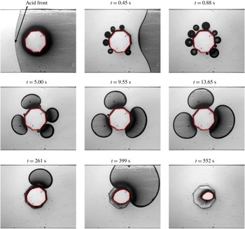
Image sequence of the formation of
 $\text{CO}_{2}$
bubbles during the acidifying process of a calcite crystal. Experimental conditions: 1 % HCl concentration,
 $6.9\times 10^{-10}~\text{m}^{3}~\text{s}^{-1}$
flow rate.
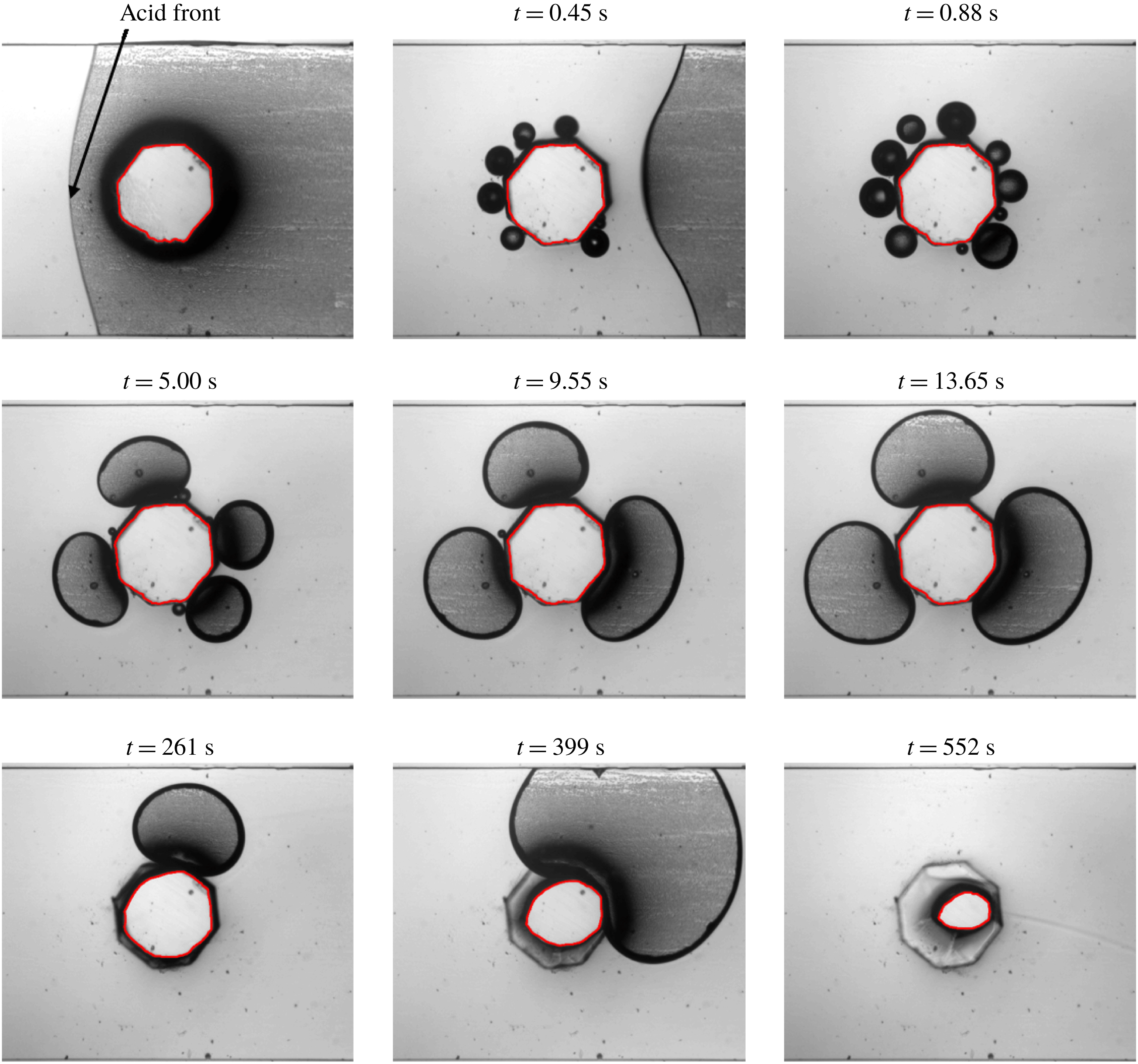
Figure 4 shows images of the calcite dissolution with production of gas bubbles at different times during the injection at
 $6.9\times 10^{-10}~\text{m}^{3}~\text{s}^{-1}$
of a solution containing 1 % of HCl. Similar results are obtained for the injection of 0.5 % of HCl at a lower rate. First, the sequence focuses on the events that occur just after the passage of the acid front, i.e. from 0 to about 15 s after the acid front reached the calcite. First, many small
 $\text{CO}_{2}$
bubbles nucleate at the crystal surface (figure 4,
 $t=0.45$
s,
 $t=0.88$
s). The nucleation sites are arranged uniformly all around the calcite surface. Then, as the chemical reaction continues, the bubbles grow and merge with their closest neighbours. After about 5 s, the bubble size distribution changes from large numbers of small bubbles to only a few – three or four – large bubbles (figure 4,
 $t=5.00$
s,
 $t=9.55$
s,
 $t=13.65$
s). The spacing between the largest bubbles remains relatively uniform. These larger bubbles are fed by smaller bubbles produced at the nucleation sites that are still exposed to the acidified aqueous phase. Some of these large bubbles come off the calcite surface, and they are transported away by the flow. At some point, one, or several, large bubbles continue to grow while no small bubbles are visible (figure 4,
 $t=13.65$
s,
 $t=261$
s,
 $t=399$
s). This suggests that very small bubbles are generated at the surface of the mineral, but migrate to the large ones before they become visible. Eventually, the large bubbles coalesce, detach and the sequence is repeated. For these experimental conditions, the calcite post is fully dissolved after 13 min. A similar behaviour is observed for the injection of 0.5 % HCl at
 $1.7\times 10^{-10}~\text{m}^{3}~\text{s}^{-1}$
(figure 6):
 $\text{CO}_{2}$
small bubbles are generated for approximately 35 s, then 3 or 4 large bubbles are observed, that will eventually coalesce and detach. In this case the calcite post is fully dissolved after approximately 50 min.
Distribution of bubble sizes over time for two experimental conditions.

Quantitative measurements of the bubble size distribution are presented in figure 5 for both experiments. For both cases, only small bubbles (blue stars and red squares) are generated in the beginning. Then, these bubbles grow and coalesce and larger bubbles appear, after 7.5 and 3.5 s, figure 5(a,b) respectively. For the greater acid concentration and greater flow rate, we observe large bubbles only after 10.5 s of injection (figure 5 b, green and purple markers) and after 40 s for the other case (figure 5 a). The same regimes of bubble generation, i.e. from a lot of very small bubbles to a couple of medium sized bubbles and to one or two very large bubbles, are observed.
Mass of calcite normalized by the initial mass (
 $t=0$
s) and mass of
 $\text{CO}_{2}$
normalized by the maximum mass of
 $\text{CO}_{2}$
that can be contained in the field of view, i.e. normalized mass of
 $\text{CO}_{2}=1$
when bubbles occupy the whole channel width. Experimental conditions: 0.5 % HCl concentration,
 $1.7\times 10^{-10}~\text{m}^{3}~\text{s}^{-1}$
flow rate.

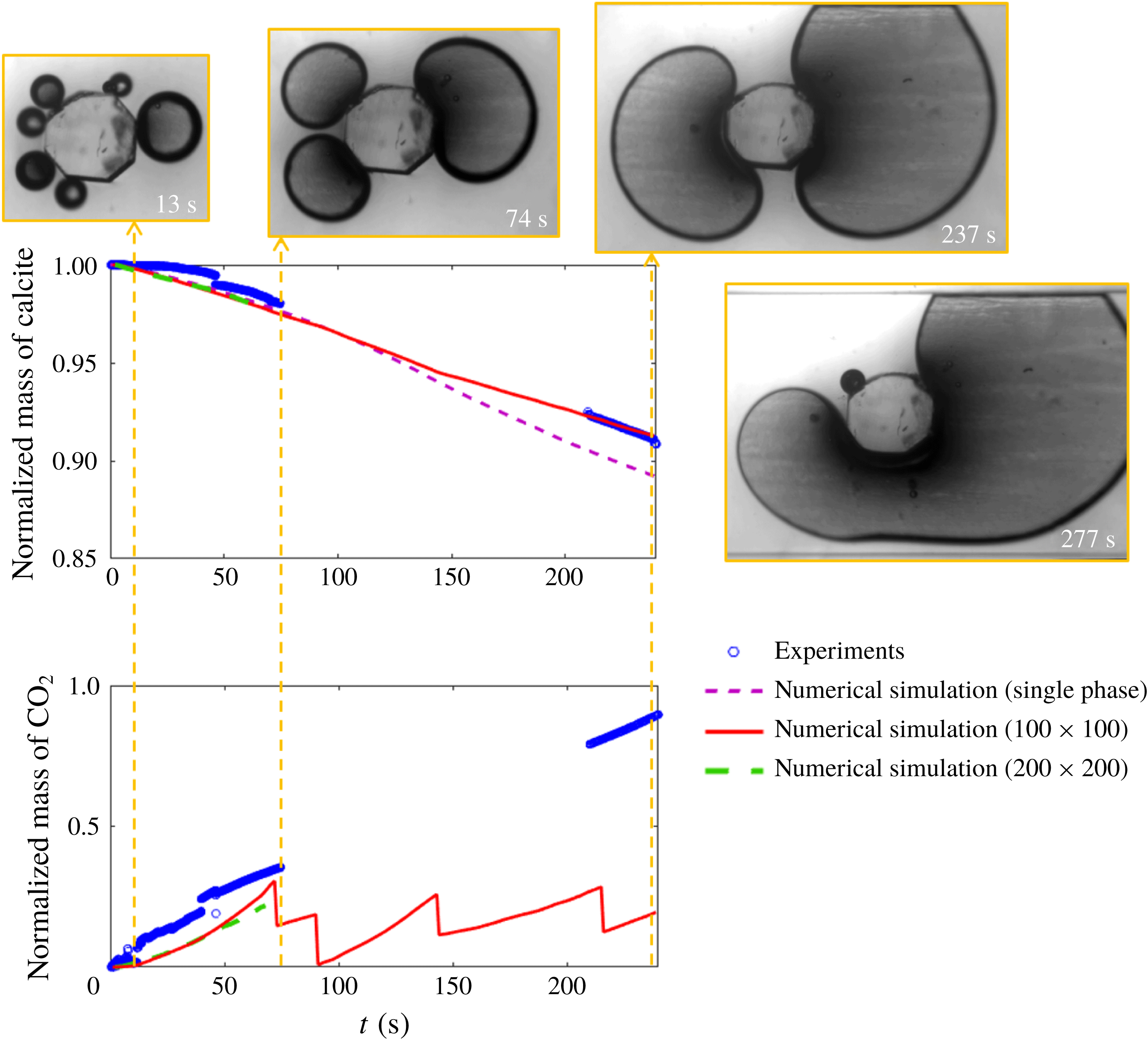
The evolution of the mass of the solid and of the gas are plotted in figure 6 for 0.5 % HCl concentration and
 $1.74\times 10^{-10}~\text{m}^{3}~\text{s}^{-1}$
flow rate. The area of the calcite normalized by the initial area is measured and is equivalent to the normalized mass of calcite. The area occupied by
 $\text{CO}_{2}$
bubbles, that are connected to the calcite, is normalized by the area of the channel in the field of view, meaning that when the gas occupies the whole space, this value is equal to 1. In figure 6 we observe that the mass of calcite decreases at a rate of approximately
 $0.025\,\%~\text{s}^{-1}$
from 0 to 300 s. At this point a very large bubble is protecting the calcite crystal from being exposed to the acid solution, see picture at 277 s on figure 6. Notes that the lack of experimental points from approximately 70 to 220 s is due to memory limitation of the camera when recording sequences of high-resolution images.
We also observe that the crystal geometry does not evolve to the petal-like shape identified during the dissolution of solid minerals under single-phase flow conditions (Molins et al.
Reference Molins, Trebotich, Miller and Steefel2017; Soulaine et al.
Reference Soulaine, Roman, Kovscek and Tchelepi2017). Instead of an elongated profile in the main direction of the flow, the shape of the crystal when
 $\text{CO}_{2}$
is produced as a separate phase is difficult to characterize and depends on the complex history of the gas bubble formation, from the nucleation to the drying of the mineral surface which stops the chemical reaction at this location.
3.3 Simulation results
The multiphase DBS framework is used to model the dissolution of the first experimental dataset (0.5 % HCl at
 $1.7\times 10^{-10}~\text{m}^{3}~\text{s}^{-1}$
). The geometry consists in a
 $1.5~\text{mm}\times 1.5~\text{mm}$
two-dimensional box that contains a cylindrical pillar in the middle. Two grids are considered: the domain is discretized by a
 $100\times 100$
Cartesian grid and by a finer
 $200\times 200$
grid. The cell porosity is set to
 $\unicode[STIX]{x1D700}=0.001$
for the cells that make up a cylinder of 0.5 mm in diameter centred in the middle of the domain. Elsewhere,
 $\unicode[STIX]{x1D700}=1$
. The top and bottom boundaries of the domain are set as impermeable fixed walls with no reaction. Initially, the domain is saturated with liquid water both in the clear-fluid region and in the porous region (
 $S_{l}=1$
everywhere). At the pillar boundary, a constant contact angle
 $\unicode[STIX]{x1D703}=45^{\circ }$
is imposed and the constant of reaction is set to
 $r=5\times 10^{-3}~\text{m}~\text{s}^{-1}$
based on the value obtained by Soulaine et al. (Reference Soulaine, Roman, Kovscek and Tchelepi2017). A solution of 0.5 % of acid is injected in the aqueous phase from the left-hand side of the domain at a constant velocity
 $v_{0}=5.8\times 10^{-4}~\text{m}~\text{s}^{-1}$
for 300 s. The right-hand side is an outflow condition. The other properties are
 $\unicode[STIX]{x1D70C}_{s}=2165~\text{kg}~~\text{m}^{-3}$
,
 $\unicode[STIX]{x1D70C}_{l}=1000~\text{kg}~~\text{m}^{-3}$
,
 $\unicode[STIX]{x1D70C}_{g}=1~\text{kg}~\text{m}^{-3}$
,
 $\unicode[STIX]{x1D707}_{l}=10^{-3}~\text{Pa}~\text{s}$
,
 $\unicode[STIX]{x1D707}_{g}=10^{-3}~\text{Pa}~\text{s}$
,
 $\unicode[STIX]{x1D70E}=0.03~\text{kg}~\text{s}^{-2}$
,
 $D_{l,A}=D_{g,A}=5\times 10^{-9}~\text{m}^{2}~\text{s}^{-1}$
,
 $H_{A}=1$
and
 $k_{0}=10^{-15}~\text{m}^{2}$
. To investigate the effect of the gas phase, simulations are also run under single-phase flow conditions assuming that the
 $\text{CO}_{2}$
produced at the mineral surface is entirely soluble in the aqueous phase.
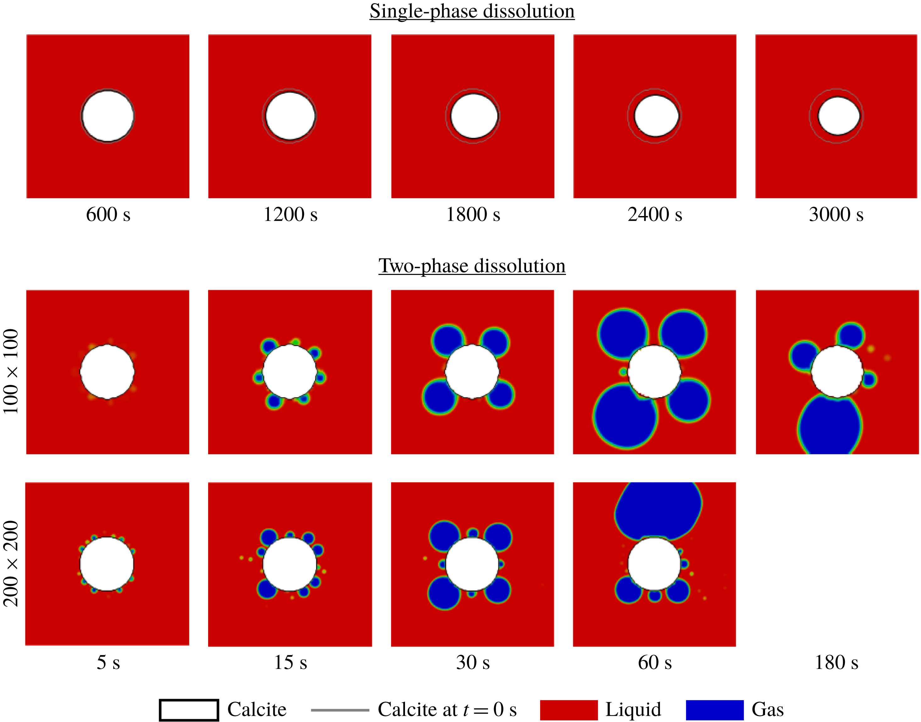
Simulation results for the evolution of a calcite grain during the injection of acid under single-phase and two-phase conditions.

Snapshots of the dissolution process are presented in figure 7 for the two grids and the single-phase dissolution. For the single-phase case, the solid grain evolves from a cylindrical shape to an oval with only one axis of symmetry. This evolution is due to the coupling with hydrodynamics and a faster dissolution rate upstream than downstream (Molins et al.
Reference Molins, Trebotich, Miller and Steefel2017; Soulaine et al.
Reference Soulaine, Roman, Kovscek and Tchelepi2017). For the multiphase simulations, the volume fraction of gas around the grain increases during the injection of acid. When enough
 $\text{CO}_{2}$
is produced, the surface tension forms small gas bubbles. Note that the interface between gas and liquid is resolved in the images when
 $S_{l}<0.5$
. The number of bubbles increases with the resolution of the computational grid. Similar to the sequence of events observed in the experiments, the bubbles grow and coalesce until three or four main bubbles occupy the domain with a uniform distribution around the calcite. The larger bubbles are fed by smaller gas bubbles that are not always visible in the image but are described with saturation between and eventually detach.
The evolution of the mass of solid and gas in the domain are plotted in figure 6 and compared with the experimental data. The prediction for the evolution of the mass of solid is in very good agreement with the experiment. Because the presence of the gas as a separate phase creates a barrier to the acid, the mean dissolution rate under two-phase condition is less important than under single-phase conditions. The rate of production of gas is also well captured by the multiphase DBS framework for the first 70 s. The sudden drops in the evolution of the mass of gas after that show, however, that the dynamics of the detachment is faster in the simulations than in the experiments. The fact that the simulations are two-dimensional while the experiment is actually three-dimensional can explain the premature detachments in the simulation. Indeed, the three-dimensional effects due to the confinement of the fluids between the top and bottom plates can play an important role in the multiphase dynamics. The modelling of the wall adhesion condition can also explain this difference and more accurate models for the contact angle could improve the prediction.
The successful comparison between the experimental measurements and the simulation results builds up confidence in the multiphase DBS predictions. In particular, the immersed boundaries used for the wettability conditions and the chemical reactions at the mineral surfaces capture the dynamics of the mineral dissolution.
4 Production of gas and evolution of wormholes
Now, we use the simulation framework of two-phase reactive transport to investigate the effect of the production of a gas phase during the injection of acid in a porous medium. The simulation set-up, i.e. the geometry, fluid and rock properties, is based on the experimental work of Song et al. (Reference Song, de Haas, Fadaei and Sinton2014). This set-up was already used in our previous study regarding the emergence of wormholes at the pore scale during mineral dissolution under single-phase flow conditions (Soulaine et al.
Reference Soulaine, Roman, Kovscek and Tchelepi2017). It consists of multiple solid pillars, approximately
 $500~\unicode[STIX]{x03BC}\text{m}\times 500~\unicode[STIX]{x03BC}\text{m}$
, distributed uniformly in a
 $24~\text{mm}\times 7.2~\text{mm}$
two-dimensional domain. The pillars are aligned and separated from each other by
 $300~\unicode[STIX]{x03BC}\text{m}$
wide vertical and horizontal channels. The porosity, permeability and specific area of the domain are
 $\unicode[STIX]{x1D719}_{0}\approx 0.76$
,
 $K_{0}=1.3\times 10^{-8}~\text{m}^{2}$
and
 $A_{0}=2310~\text{m}^{-1}$
, respectively.
The computational domain is meshed using a
 $500\times 150$
Cartesian grid. The top and bottom boundaries are set as impermeable walls. Two per cent of acid are injected from the left-hand side of the domain at a constant velocity
 $v_{0}=10^{-3}~\text{m}~\text{s}^{-1}$
corresponding to
 $Re=\unicode[STIX]{x1D70C}_{l}\sqrt{K_{0}}v_{0}/\unicode[STIX]{x1D707}_{l}\approx 0.1$
during approximately 4 min. The right-hand side is an outflow condition. At the pillar boundary, a constant contact angle
 $\unicode[STIX]{x1D703}=45^{\circ }$
is imposed and the constant of reaction is set to
 $r=5\times 10^{-3}~\text{m}~\text{s}^{-1}$
. Two cases are considered. First, the two-phase reactive transport simulation framework is used to investigate the dissolution of minerals in porous media with production of
 $\text{CO}_{2}$
that forms gas bubbles, limiting the dissolution process. In this case, simulation properties are set to
 $\unicode[STIX]{x1D707}_{l}=10^{-3}~\text{Pa}~\text{s}$
,
 $\unicode[STIX]{x1D70C}_{l}=1000~\text{kg}~\text{m}^{-3}$
,
 $\unicode[STIX]{x1D707}_{g}=10^{-3}~\text{Pa}~\text{s}$
,
 $\unicode[STIX]{x1D70C}_{g}=1~\text{kg}~\text{m}^{-3}$
,
 $\unicode[STIX]{x1D70E}=10~\text{mN}~\text{m}^{-1}$
,
 $D_{l,A}=D_{g,A}=5\times 10^{-9}~\text{m}^{2}~\text{s}^{-1}$
,
 $H_{A}=1$
,
 $\unicode[STIX]{x1D70C}_{s}=2165~\text{kg}~\text{m}^{-3}$
and
 $k_{0}=10^{-15}~\text{m}^{2}$
. In the second case, we consider that all the
 $\text{CO}_{2}$
dissolves instantaneously in the aqueous phase. This is achieved using the same framework with
 $\unicode[STIX]{x1D70E}=0~\text{mN}~\text{m}^{-1}$
,
 $\unicode[STIX]{x1D70C}_{g}=\unicode[STIX]{x1D70C}_{l}=1000~\text{kg}~\text{m}^{-3}$
,
 $\unicode[STIX]{x1D707}_{g}=\unicode[STIX]{x1D707}_{l}=10^{-3}~\text{Pa}~\text{s}$
and
 $a_{v}^{l}=a_{v}$
instead of
 $a_{v}^{l}=a_{v}S_{l}$
.
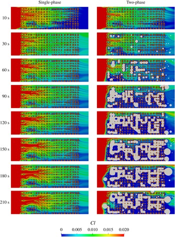
Evolution of a porous medium during the injection of acid. The colour map corresponds to the concentration of acid in the domain. Solid grains are depicted in brown. (a) Under single-phase flow conditions, the acid penetrates the domain and dissolves the solid grains producing wormholes. (b) The mineral dissolution generates
 $\text{CO}_{2}$
gas that occupies the pore space, limits the dissolution process and prevents the development of wormholes.
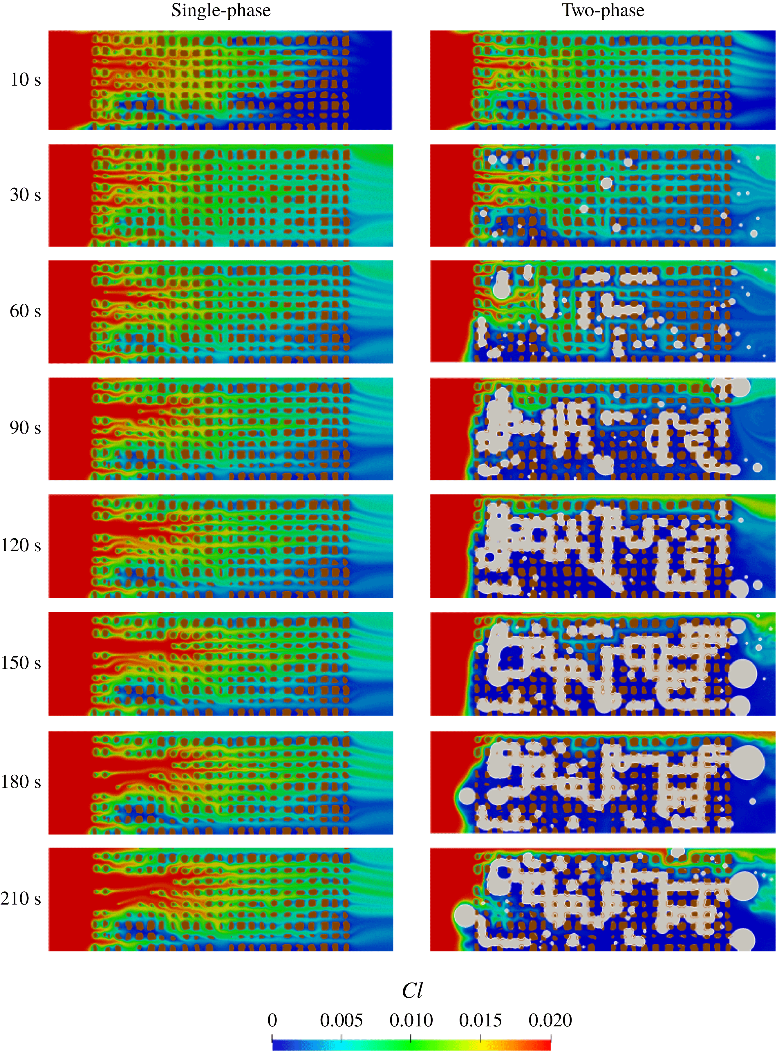
Under single-phase flow conditions, it is now well established that five different dissolution patterns exist according to the constant of reaction at the mineral surface and the injection mass flow rate, namely compact dissolution, conical dissolution, one dominant wormhole, ramified wormholes and uniform dissolution (Golfier et al.
Reference Golfier, Zarcone, Bazin, Lenormand, Lasseux and Quintard2002; Szymczak & Ladd Reference Szymczak and Ladd2009; Soulaine et al.
Reference Soulaine, Roman, Kovscek and Tchelepi2017). These regimes are usually characterized by the Péclet (
 $P\acute{e} =v_{0}\sqrt{K_{0}}/D_{l,A}$
) and the Damköhler (
 $Da_{II}=rA_{0}^{-1}/D_{l,A}$
) numbers. Here,
 $P\acute{e} \approx 22$
and
 $Da_{II}\approx 432$
that correspond to the wormhole regime. The objective of these simulations is to investigate the effect of the production of gas bubbles on the emergence of wormholes in the domain. The simulation results at different times for both cases are presented in figure 8. As expected for the single-phase flow conditions, regions of preferential flow induced by local heterogeneities of the porous medium lead to a non-uniform distribution of the acid concentration in the domain and subsequently to the emergence of wormholes.
For two-phase flow conditions, the chemical reactions at the grain boundaries generate
 $\text{CO}_{2}$
that form a separate phase. Some gas bubbles detach and flow out of the domain. Others occupy pores and continue to grow. When they filled the entire volume of the pore, bubbles from adjacent pores connect and coalesce forming larger clusters. The clusters of gas are flow barriers that limit the distribution of the acid concentration in the domain. The sequence from 10 to 60 s illustrates well this process: at 30 s, the bubbles in the second row from the top stop the propagation of the acid in the domain, and at 60 s the two first bubbles in this row have grown, coalesced and are moving to a location where the surface energy of the bubble is less important, i.e. in a larger pore. The dissolution of the minerals continues while releasing
 $\text{CO}_{2}$
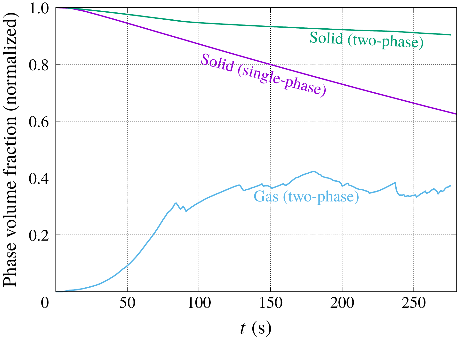
. Eventually, a large cluster occupies the pore space. The evolution of the average gas saturation in the porous medium is plotted in figure 9. The amount of gas in the domain increases monotonically until approximately 80 s where a gas cluster detaches and flow out of the domain. The volume of gas stabilizes to approximately 40 % of the pore space which corresponds to the indications of Thompson & Gdanski (Reference Thompson and Gdanski1993).
The large
 $\text{CO}_{2}$
clusters limit the flow and subsequently the propagation of the acid in the domain. We see in figure 8 that after 80 s, the acid has dissolved the first column and the first row of pillar mainly, slowing down significantly the average dissolution rate and preventing the development of wormholes in the domain. The evolution of the mass of solid normalized by the initial mass is plotted in figure 9 for both the single- and the two-phase conditions. We observe that the dissolution rate is strongly impacted by the presence of gas in the domain: after 4 min, 32.4 % of the solid is dissolved in the single flow set-up, while this is only 8.5 % in the two-phase flow set-up.
Evolution of the amount of solid and gas in the system for both the single-phase and two-phase flow conditions.

The simulations presented here emphasize the importance of considering the production of a gas phase in the modelling of acid stimulation processes. As suggested by the experiments of Ott & Oedai (Reference Ott and Oedai2015), dissolution during single-phase flow condition produces wormholes; however, the presence of a second fluid phase under the same flow conditions may lead to very different dissolution regimes. Behaviour diagrams that characterize the dissolution pattern based on the Péclet and Damköhler numbers (Golfier et al.
Reference Golfier, Zarcone, Bazin, Lenormand, Lasseux and Quintard2002) have to be complemented, at a minimum, by a third dimension that quantifies the solubility of the
 $\text{CO}_{2}$
in the aqueous phase.
5 Conclusions
We extended the micro-continuum DBS model proposed by Soulaine et al. (Reference Soulaine, Roman, Kovscek and Tchelepi2017) to the presence of two fluid phases. The framework is used to simulate the complex pore-scale reactive transport associated with dissolution dynamics of carbonates. The model uses a combination of the Darcy–Brinkman–Stokes equation and the volume of fluid (VOF) method, and accounts for the surface-tension force. Chemical reactions and wettability conditions at the mineral surface are described as immersed boundaries that evolve with the dissolution of the solid phase. The multiphase micro-continuum model is implemented in the finite-volume OpenFOAM® simulation framework.
The simulation framework is validated using an experimental microfluidic device to image and analyse the dissolution of a single calcite crystal, and the subsequent generation of
 $\text{CO}_{2}$
bubbles in the domain. The same sequence of events is observed for different flow conditions. First, a multitude of small gas bubbles nucleate at the solid surface. Second, as the bubbles grow, they coalesce with each other and their number decreases significantly until three or four large bubbles are visible. As the bubbles grow, the gas phase covers a larger surface of the solid and prevents the acid from reacting with the mineral. Eventually, large bubbles detach, and the whole sequence is repeated. The multiphase micro-continuum model was able to capture accurately the sequence of events. In particular, the immersed boundaries used for the wettability conditions and the chemical reactions at the mineral surfaces capture the dynamics of the mineral dissolution under multiphase flow conditions.
The micro-continuum model was then used to investigate the effect of
 $\text{CO}_{2}$
production during the acidization of carbonate formations. Under single-phase flow conditions, i.e. when the dissolution time of
 $\text{CO}_{2}$
into the aqueous phase is instantaneous, the solid structure dissolves forming wormholes. However, if the characteristic time scale of
 $\text{CO}_{2}$
dissolving in brine is much longer compared with the rate of gas production, then the simulation results show that
 $\text{CO}_{2}$
bubbles grow, coalesce and form flow barriers that limit the transport of the acid in the domain. These flow barriers prevent the emergence of wormholes and limit significantly the overall dissolution rate.
Further improvements of the model include accounting for gas compressibility, diffusion-induced phase separation between the liquid and the gas, and dynamic contact angle changes due to the evolution of the surface roughness during minerals dissolution.
Acknowledgements
We acknowledge the Office of Basic Energy Sciences Energy Frontier Research Center under contract number DE-AC02-05CH11231 and the TOTAL STEMS project for financial support. We thank the Stanford Center for Computational Earth & Environmental Sciences (CEES) for computational support. The authors also acknowledge Ms W. Song (Stanford University) for discussions regarding the reactive microfluidic apparatus.
Appendix A. Derivation of the saturation equation
Here, we derive the saturation equation from the conservation law for the liquid phase. We have,
 $$\begin{eqnarray}\displaystyle \frac{\unicode[STIX]{x2202}\unicode[STIX]{x1D700}_{l}\unicode[STIX]{x1D70C}_{l}}{\unicode[STIX]{x2202}t}+\unicode[STIX]{x1D735}\boldsymbol{\cdot }(\unicode[STIX]{x1D700}_{l}\unicode[STIX]{x1D70C}_{l}\bar{\mathsf{v}}_{l})=\dot{m_{l}}. & & \displaystyle\end{eqnarray}$$
Because the liquid is incompressible and because
 $\unicode[STIX]{x1D700}_{l}=\unicode[STIX]{x1D700}S_{l}$
and
 $S_{l}+S_{g}=1$
, equation (A 1) can be recast into,
 $$\begin{eqnarray}\displaystyle & \displaystyle \frac{\unicode[STIX]{x2202}\unicode[STIX]{x1D700}S_{l}}{\unicode[STIX]{x2202}t}+\unicode[STIX]{x1D735}\boldsymbol{\cdot }(\unicode[STIX]{x1D700}S_{l}(S_{l}+S_{g})\bar{\mathsf{v}}_{l})=\frac{\dot{m_{l}}}{\unicode[STIX]{x1D70C}_{l}}, & \displaystyle\end{eqnarray}$$
 $$\begin{eqnarray}\displaystyle & \displaystyle \frac{\unicode[STIX]{x2202}\unicode[STIX]{x1D700}S_{l}}{\unicode[STIX]{x2202}t}+\unicode[STIX]{x1D735}\boldsymbol{\cdot }(\unicode[STIX]{x1D700}S_{l}S_{l}\bar{\mathsf{v}}_{l})+\unicode[STIX]{x1D735}\boldsymbol{\cdot }(\unicode[STIX]{x1D700}S_{l}S_{g}\bar{\mathsf{v}}_{l})=\frac{\dot{m_{l}}}{\unicode[STIX]{x1D70C}_{l}}, & \displaystyle\end{eqnarray}$$
 $$\begin{eqnarray}\displaystyle & \displaystyle \frac{\unicode[STIX]{x2202}\unicode[STIX]{x1D700}S_{l}}{\unicode[STIX]{x2202}t}+\unicode[STIX]{x1D735}\boldsymbol{\cdot }(\unicode[STIX]{x1D700}S_{l}(S_{l}\bar{\mathsf{v}}_{l}+S_{g}\bar{\mathsf{v}}_{g}))+\unicode[STIX]{x1D735}\boldsymbol{\cdot }(\unicode[STIX]{x1D700}S_{l}S_{g}(\bar{\mathsf{v}}_{l}-\bar{\mathsf{v}}_{g}))=\frac{\dot{m_{l}}}{\unicode[STIX]{x1D70C}_{l}}. & \displaystyle\end{eqnarray}$$
By definition of the total velocity and relative velocity, we have
 $\bar{\mathsf{v}}=\unicode[STIX]{x1D700}(S_{l}\bar{\mathsf{v}}_{l}+S_{g}\bar{\mathsf{v}}_{g})$
and
 $\bar{\mathsf{v}}_{r}=(\bar{\mathsf{v}}_{l}-\bar{\mathsf{v}}_{g})$
respectively. Finally, the saturation equation is,
 $$\begin{eqnarray}\displaystyle \frac{\unicode[STIX]{x2202}\unicode[STIX]{x1D700}S_{l}}{\unicode[STIX]{x2202}t}+\unicode[STIX]{x1D735}\boldsymbol{\cdot }(\bar{\mathsf{v}}S_{l})+\unicode[STIX]{x1D735}\boldsymbol{\cdot }(\unicode[STIX]{x1D700}S_{l}(1-S_{l})\bar{\mathsf{v}}_{r})=\frac{\dot{m_{l}}}{\unicode[STIX]{x1D70C}_{l}}. & & \displaystyle\end{eqnarray}$$
Appendix B. Normal to the gas/liquid interface locally modified to account for wall adhesion condition
We have,
 $$\begin{eqnarray}\displaystyle \boldsymbol{n}_{lg}=\cos \unicode[STIX]{x1D703}_{I}\boldsymbol{n}_{wall}+\sin \unicode[STIX]{x1D703}_{I}\boldsymbol{t}_{wall} & & \displaystyle\end{eqnarray}$$
and we want,
 $$\begin{eqnarray}\displaystyle \hat{\boldsymbol{n}}_{lg}=\cos \unicode[STIX]{x1D703}\boldsymbol{n}_{wall}+\sin \unicode[STIX]{x1D703}\boldsymbol{t}_{wall}. & & \displaystyle\end{eqnarray}$$
The multiplication of (B 1) by
 $\sin \unicode[STIX]{x1D703}_{I}$
leads to,
 $$\begin{eqnarray}\displaystyle \boldsymbol{t}_{wall}=\frac{\sin \unicode[STIX]{x1D703}_{I}}{\sin ^{2}\unicode[STIX]{x1D703}_{I}}\boldsymbol{n}_{lg}-\frac{\cos \unicode[STIX]{x1D703}_{I}\sin \unicode[STIX]{x1D703}_{I}}{\sin ^{2}\unicode[STIX]{x1D703}_{I}}\boldsymbol{n}_{wall} & & \displaystyle\end{eqnarray}$$
that can be recast into,
 $$\begin{eqnarray}\displaystyle \boldsymbol{t}_{wall}=\frac{\sin \unicode[STIX]{x1D703}_{I}}{1-\cos ^{2}\unicode[STIX]{x1D703}_{I}}\boldsymbol{n}_{lg}-\frac{\cos \unicode[STIX]{x1D703}_{I}\sin \unicode[STIX]{x1D703}_{I}}{1-\cos ^{2}\unicode[STIX]{x1D703}_{I}}\boldsymbol{n}_{wall}. & & \displaystyle\end{eqnarray}$$
Combining (B 2) and (B 4), we have,
 $$\begin{eqnarray}\displaystyle \hat{\boldsymbol{n}}_{lg}=\left(\cos \unicode[STIX]{x1D703}-\frac{\sin \unicode[STIX]{x1D703}\sin \unicode[STIX]{x1D703}_{I}\cos \unicode[STIX]{x1D703}_{I}}{1-\cos ^{2}\unicode[STIX]{x1D703}_{I}}\right)\boldsymbol{n}_{wall}+\left(\frac{\sin \unicode[STIX]{x1D703}\sin \unicode[STIX]{x1D703}_{I}}{1-\cos ^{2}\unicode[STIX]{x1D703}_{I}}\right)\boldsymbol{n}_{lg}. & & \displaystyle\end{eqnarray}$$
Finally, with simple algebra, we have,
 $$\begin{eqnarray}\displaystyle \hat{\boldsymbol{n}}_{lg}=\left(\frac{\cos \unicode[STIX]{x1D703}-\cos \unicode[STIX]{x1D703}_{I}\cos (\unicode[STIX]{x1D703}_{I}-\unicode[STIX]{x1D703})}{1-\cos ^{2}\unicode[STIX]{x1D703}_{I}}\right)\boldsymbol{n}_{wall}+\left(\frac{\cos (\unicode[STIX]{x1D703}_{I}-\unicode[STIX]{x1D703})-\cos \unicode[STIX]{x1D703}_{I}\cos \unicode[STIX]{x1D703}}{1-\cos ^{2}\unicode[STIX]{x1D703}_{I}}\right)\boldsymbol{n}_{lg}. & & \displaystyle\end{eqnarray}$$
Appendix C. Numerical implementation
The model proposed in this paper is implemented in the open-source computational fluid dynamics (CFD) platform OpenFOAM®. This code is a C++ library that solves partial differential equations with the finite-volume method. It handles complex three-dimensional grids by default and has demonstrated a good scalability for parallel computing of flow in porous media (Orgogozo et al. Reference Orgogozo, Renon, Soulaine, Hénon, Tomer, Labat, Pokrovsky, Sekhar, Ababou and Quintard2014; Guibert et al. Reference Guibert, Nazarova, Horgue, Hamon, Creux and Debenest2015; Horgue et al. Reference Horgue, Soulaine, Franc, Guibert and Debenest2015). One of its features is to solve the coupled equations using sequential approaches. This section details the solution algorithm developed in this paper. Close attention is paid to the velocity–pressure coupling.
C.1 Discretization of the equations
The momentum equation, equation (2.15), is transformed into a set of algebraic equations after application of the finite-volume discretization procedure. The nonlinearity introduced by the advection term is dealt with by linearizing around the latest velocity field. Using the Euler implicit difference scheme and denoting successive time levels by
 $k$
and
 $k+1$
, the semi-discrete form of the momentum equation can be written as:
 $$\begin{eqnarray}\displaystyle {\mathcal{V}}\left(\frac{\unicode[STIX]{x1D70C}^{k+1}\boldsymbol{v}_{P}^{k+1}-\unicode[STIX]{x1D70C}^{k}\boldsymbol{v}_{P}^{k}}{\unicode[STIX]{x1D6FF}t}\right)=-a_{P}^{\prime }\boldsymbol{v}_{P}^{k+1}+\mathop{\sum }_{NP}a_{NP}^{\prime }\boldsymbol{v}_{NP}^{k+1}-\unicode[STIX]{x1D735}p+\boldsymbol{F}_{c}-K_{fs}\boldsymbol{v}_{P}^{k+1}. & & \displaystyle\end{eqnarray}$$
In this equation,
 ${\mathcal{V}}$
and
 $\unicode[STIX]{x1D6FF}t$
respectively stand for the cell volume and the time step. The subscript
 $P$
indicates values at the cell centre, and the coefficients
 $a_{NP}^{\prime }$
account for the influence of neighbouring control volumes. They are mainly composed by convective and diffusive fluxes across cell faces.
 $K_{fs}$
corresponds to the exchange of momentum of the fluid with regard to the solid structure (the Darcy term in (2.15)). The pressure gradient is not discretized at this stage.
All the explicit source terms other than the pressure gradient and the capillary force, i.e. here the source part of the transient term, are lumped into a single vector,
 $\boldsymbol{S}={\mathcal{V}}\unicode[STIX]{x1D70C}^{k}\boldsymbol{v}_{P}^{k}/\unicode[STIX]{x1D6FF}t$
. Equation (C 1) can be rearranged as,
 $$\begin{eqnarray}\displaystyle \left(\frac{{\mathcal{V}}\unicode[STIX]{x1D70C}^{k+1}}{\unicode[STIX]{x1D6FF}t}+a_{P}^{\prime }+K_{fs}\right)\boldsymbol{v}_{P}^{k+1}=\mathop{\sum }_{NP}a_{NP}^{\prime }\boldsymbol{v}_{NP}^{k+1}+\boldsymbol{S}-\unicode[STIX]{x1D735}p+\boldsymbol{F}_{c}. & & \displaystyle\end{eqnarray}$$
This equation forms a matrix system that results from the momentum equation discretization. The term,
 $a_{P}=(({\mathcal{V}}\unicode[STIX]{x1D70C}^{k+1}/\unicode[STIX]{x1D6FF}t)+a_{P}^{\prime }+K_{fs})$
, represents the diagonal term of this matrix. Following OpenFOAM® internal notations, the operator
 $\boldsymbol{H}(\boldsymbol{X})=\sum _{NP}a_{NP}^{\prime }\boldsymbol{X}_{NP}+\boldsymbol{S}$
is introduced (Jasak Reference Jasak1996) and (C 2) turns into,
 $$\begin{eqnarray}\displaystyle a_{P}\boldsymbol{v}_{P}^{k+1}=\boldsymbol{H}(\boldsymbol{v}^{k+1})-\unicode[STIX]{x1D735}p+\boldsymbol{F}_{c}. & & \displaystyle\end{eqnarray}$$
This semi-discretized form of the momentum balance is used to form the pressure equation. This is usually achieved by dividing (C 3) by the diagonal coefficient,
 $a_{P}$
, and substituting the semi-discretized form of
 $\boldsymbol{v}^{k+1}$
into the overall mass balance, equation (2.13). Finally, the pressure equation can be written as:
 $$\begin{eqnarray}\displaystyle \unicode[STIX]{x1D735}\boldsymbol{\cdot }\left(\frac{\boldsymbol{H}(\boldsymbol{v}^{k+1})+\boldsymbol{F}_{c}}{a_{P}}\right)-\unicode[STIX]{x1D735}\boldsymbol{\cdot }\left(\frac{1}{a_{P}}\unicode[STIX]{x1D735}p^{k+1}\right)={\dot{m}}_{l,HCl}\left(\frac{\unicode[STIX]{x1D6FE}_{l}}{\unicode[STIX]{x1D70C}_{l}}+\frac{\unicode[STIX]{x1D6FE}_{g}}{\unicode[STIX]{x1D70C}_{g}}+\frac{\unicode[STIX]{x1D6FE}_{s}}{\unicode[STIX]{x1D70C}_{s}}\right). & & \displaystyle\end{eqnarray}$$
The transport equation for species, equation (2.21), is also discretized following a similar procedure. For a better accuracy of the results, convection terms are discretized with a van Leer scheme. Further details regarding the discretization procedure in OpenFOAM® can be found in Jasak (Reference Jasak1996), Weller et al. (Reference Weller, Tabor, Jasak and Fureby1998). The saturation, equation (2.14), is discretized with a van Leer limiter function for the convection term and a forward Euler for time discretization.
C.2 Solution algorithm
Schematic of the sequential algorithm.

The discretized equations are solved with OpenFOAM® in a segregated way. In particular, the pressure–velocity coupling formed by (C 3) and (C 4) is handled by a predictor–corrector algorithm along the same lines as the pressure implicit splitting-operator (PISO) algorithm originally designed by Issa (Reference Issa1985) to solve the transient Navier–Stokes equations. Our implementation follows guidelines proposed for the simulations of multiphase system with gas/liquid phase change during boiling processes (Juric & Tryggvason Reference Juric and Tryggvason1998; Welch & Wilson Reference Welch and Wilson2000; Guo et al. Reference Guo, Sun, Li and Tao2011). It is built on the top of the OpenFOAM® VOF solver interFoam. The main steps are described below and sketched in figure 10.
(i) Each mass balance equations for species, equation (2.21), is computed sequentially. The advection terms are based on the velocity,
 $\boldsymbol{v}^{k}$
, of the previous time step and all these equations are solved implicitly with regard to their main variable. At the end of this first step, the reaction rates for species
${\dot{m}}_{l,A}$
and phases
$\dot{m_{i}}$
(with
$i=s,g,l$
) are computed with (2.24) and (2.9), respectively.
(ii) Evolution of the volume fraction of solid solving (2.10).
(iii) The saturation, equation (2.14), is solved explicitly using the OpenFOAM® implementation of the flux corrected transport (FCT) theory (Rudman Reference Rudman1997) called multidimensional universal limiter with explicit solution (MULES). Details regarding the MULES algorithm can be found in Damian (Reference Damian2013) chap. 5.
(iv) Update of the micro-permeability
$k$
and the dispersion tensor
$D_{A}^{\ast }$
using (2.16) and (2.22) with the new value of
$\unicode[STIX]{x1D700}$
and
$S_{l}$
. The density,
$\unicode[STIX]{x1D70C}$
, and viscosity,
$\unicode[STIX]{x1D707}$
, are also updated with the new value of the saturation field. The surface-tension force,
$\boldsymbol{F}_{c}^{k+1}$
, is computed using (2.17) and (2.19).(v) The next stage consists in the prediction of the velocity field,
$\boldsymbol{v}^{\ast }$
, by solving implicitly the momentum equation, (C 5)where the gradient of the pressure field is evaluated from the values computed at the previous time step. This stage is called the momentum predictor. Actually, if the time step is small enough, it is not even necessary to solve this equation and only an update of$$\begin{eqnarray}\displaystyle a_{P}\boldsymbol{v}_{P}^{\ast }=\boldsymbol{H}(\boldsymbol{v}^{\ast })+\boldsymbol{F}_{c}^{k+1}-\unicode[STIX]{x1D735}p^{k}, & & \displaystyle\end{eqnarray}$$
$a_{P}$
and
$\boldsymbol{H}(\boldsymbol{v})$
with the latest computed velocity profile is necessary.(vi) The predicted velocity
$\boldsymbol{v}^{\ast }$
does not satisfy the continuity equation (2.13) and has to be corrected. This is achieved by looking for
$(\boldsymbol{v}^{\ast \ast },p^{\ast })$
that obeys, (C 6)$$\begin{eqnarray}\displaystyle & \displaystyle \boldsymbol{v}_{P}^{\ast \ast }=\frac{1}{a_{P}}[\boldsymbol{H}(\boldsymbol{v}^{\ast })+\boldsymbol{F}_{c}^{k+1}-\unicode[STIX]{x1D735}p^{\ast }], & \displaystyle\end{eqnarray}$$
(C 7)Assembling these two equations, the pressure equation can be formulated as$$\begin{eqnarray}\displaystyle & \displaystyle \unicode[STIX]{x1D735}\boldsymbol{\cdot }\boldsymbol{v}^{\ast \ast }={\dot{m}}_{l,HCl}\left(\frac{\unicode[STIX]{x1D6FE}_{l}}{\unicode[STIX]{x1D70C}_{l}}+\frac{\unicode[STIX]{x1D6FE}_{g}}{\unicode[STIX]{x1D70C}_{g}}+\frac{\unicode[STIX]{x1D6FE}_{s}}{\unicode[STIX]{x1D70C}_{s}}\right). & \displaystyle\end{eqnarray}$$
(C 8)and solved implicitly with a generalized method of geometric-algebraic multi-grid (GAMG) embedded in OpenFOAM®. The corrected velocity$$\begin{eqnarray}\displaystyle \unicode[STIX]{x1D735}\boldsymbol{\cdot }\left(\frac{\boldsymbol{H}(\boldsymbol{v}^{\ast })+\boldsymbol{F}_{c}^{k+1}}{a_{P}}\right)-\unicode[STIX]{x1D735}\boldsymbol{\cdot }\left(\frac{1}{a_{P}}\unicode[STIX]{x1D735}p^{\ast }\right)={\dot{m}}_{l,HCl}\left(\frac{\unicode[STIX]{x1D6FE}_{l}}{\unicode[STIX]{x1D70C}_{l}}+\frac{\unicode[STIX]{x1D6FE}_{g}}{\unicode[STIX]{x1D70C}_{g}}+\frac{\unicode[STIX]{x1D6FE}_{s}}{\unicode[STIX]{x1D70C}_{s}}\right), & & \displaystyle\end{eqnarray}$$
$\boldsymbol{v}^{\ast \ast }$
is then computed pointwise from (C 6). This second step, called the PISO loop, may be repeated several times to force the convergence. Issa (Reference Issa1985) demonstrates that at least two iterations are necessary to ensure that the solution of the pressure–velocity
$(\boldsymbol{v},p)$
coupling satisfies the mass conservation. The resulting values are set to
$(\boldsymbol{v}^{k+1},p^{k+1})$
and then the algorithm marches in time.