



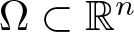



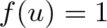
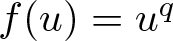
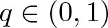






1. Introduction
In the 1970s and 1980s, significant progress was made in understanding the convexity and concavity properties of solutions to certain elliptic differential equations on convex domains and Dirichlet boundary conditions. In the pivotal papers by Brascamp and Lieb [Reference Brascamp and Lieb12] and Makar-Limanov [Reference Makar-Limanov58], the authors showed that solutions of the eigenfunction problem and of the torsion problem are concave up to a composition, respectively, with the logarithm function or the square root function. The seminal papers by Korevaar [Reference Korevaar51] and Kennington [Reference Kennington49] gave a new boost to this research by introducing general concavity maximum principles to deal with general classes of equations. We refer to [Reference Almousa, Assettini, Gallo and Squassina2, Reference Gallo and Squassina32] and references therein for a general overview of the topic. Let us mention, among various mathematical applications, that in [Reference Singer, Wong, Yau and Yau64] the authors exploit the  $\log$-concavity of the eigenfunction to show notable results about the eigenvalue gap, i.e. the difference between the first and the second Dirichlet eigenvalue.
In the framework of parabolic equations and Cauchy–Dirichlet problems
 \begin{equation*}
\begin{cases}
u_t - \Delta u = b(x,u,t) & \quad \hbox{in}\ \Omega \times (0,T),\\
u=0 & \quad \hbox{on}\ \partial \Omega \times [0,T), \\
u=u_0& \quad \hbox{on}\ \overline{\Omega} \times \{0\},
\end{cases}
\end{equation*}
 $T \in (0, +\infty]$, several questions arise. A first problem is to study very particular examples of
 $b$ and discuss if, under suitable assumptions on
 $u_0$, the solution
 $u(x,t)$ becomes logarithmic or power concave (i.e.
 $\log(u)$ or
 $u^\alpha$ for some
 $\alpha \gt 0$ is concave) after some amount of time (
 $t \gt 0$ or possibly
 $t\gg 0$): these kinds of results are strongly related to the particular shape of
 $b$ which allows, for instance, explicit representation of the solution, and have been investigated, for example, in [Reference Ishige39, Reference Lee and Vázquez54, Reference Lee and Vázquez55]. We highlight that these results allow, under suitable assumptions, to get interesting properties also in the elliptic case, by considering the limit of
 $u(x,t)$ as
 $t\to +\infty$, which coincides with the solution of the corresponding stationary problem.
A second question is the following: what is the optimal (in some sense) concavity on  $u_0$ which is preserved by the heat flow? In this problem, the logarithmic concavity plays a very special role. This and similar questions have been addressed in a series of papers [Reference Ishige and Salani41, Reference Ishige, Salani and Takatsu44–Reference Ishige, Salani and Takatsu46]. See also [Reference Chau and Weinkove17, Reference Daskalopoulos, Hamilton and Lee26] for similar questions regarding power concavity and porous medium flow.
In this paper, we are interested in a different question: under which assumptions on  $b$ and
 $u_0$ can we obtain that
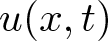 $u(x,t)$ enjoys some concavity properties for each
 $t \gt 0$? To the authors’ knowledge, only a few papers deal with this problem.
A first result can be found in Korevaar [Reference Korevaar51], where the author adapts the elliptic concavity maximum principles to study classes of parabolic equations and show that, for example, the parabolic eigenfunctions  $u(\cdot, t)$ are spatially logarithmic concave for each
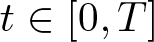 $t \in [0,T]$ if
 $u_0$ is so. Let us mention that in [Reference Andrews and Clutterbuck6] a stronger notion of
 $\log$-concavity is proved and it is exploited to prove a sharp result on the eigenvalue gap; it is notable to observe that the technique adopted in [Reference Andrews and Clutterbuck6] relies on the introduction and analysis of some suitable multivariable function in a spirit relatable to the one introduced in [Reference Kennington49, Reference Korevaar51] and used in the present paper. Some partial generalizations of the results in [Reference Korevaar51] can be found in [Reference Porru and Serra62] (see also [Reference Greco and Kawohl35]), by allowing the inclusion of other interesting models. Other results are contained in [Reference Ishige, Salani and Takatsu44] (see e.g. Proposition 4.2 therein) by means of spatial log-concave envelopes as viscosity subsolutions of the problem and corresponding comparison principles; similar techniques go back to [Reference Alvarez, Lasry and Lions4] (see also [Reference Colesanti, Qin and Salani23]).
A second result, i.e. a parabolic generalization for equations in the spirit of the torsion and Lane–Emden problems, which allows us to obtain power concavity (stronger than logarithmic one), appears first in [Reference Kennington48]: here the author studies the case  $a=1$ and
 $f(u)=(1-u)^q$,
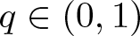 $q \in (0,1)$, obtaining that a suitable transformation of
 $u$ is concave and thus
 $u$ is quasi-concave (i.e. the superlevel sets of
 $u$ are convex). To gain the claim, the author exploits some concavity maximum principle again, and he strongly uses that
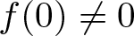 $f(0) \neq 0$ coupled with some comparison principle; moreover, he relies on the information at infinity given by the stationary problem. Other results have been more recently obtained in [Reference Ishige and Salani42, Reference Ishige and Salani43] (see also [Reference Ishige, Liu and Salani40]): here the authors rely on the use of parabolic concave envelopes as viscosity subsolutions. In such a way, the authors are able to study the concavity of nondecreasing solutions with controlled behaviour on the boundary, in the case of nonnegative nonlinearities satisfying a priori some comparison principle, set in smooth domains: for example, they cover the cases
 $f=1$, or
 $a=1$ and
 $f(u)=u^q$,
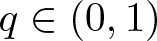 $q \in (0,1)$. Moreover, the authors study a rescaled concavity in space and time, namely they show that
 $(x,t) \mapsto u(x,t^{\beta})$ is power concave for suitable values of
 $\beta$.
The aim of this paper is twofold. First, we aim to recover and slightly generalize the abovementioned results, in a unified way, by means of parabolic concavity maximum principles. In particular, to recover the results previously obtained through different techniques, we need a finer analysis, especially regarding the boundary behaviour of the solution (including  $t \to +\infty$). A second goal is to derive quantitative estimates of concavity maximum principles, which will require a careful study of the objects in play. For the sake of clarity in presentation, we describe first some applications of the exact results (which are indeed a consequence of the quantitative estimates).
Notation. We say that  $u$ is
 $\alpha$-concave if
 $\alpha \gt 0$ and
 $u^{\alpha}$ is concave, or
 $\alpha=0$ and
 $\log(u)$ is concave (see (3.4)). Moreover, a solution of a PDE is meant positive when
 $u \gt 0$ in
 $\Omega\times (0,T]$. For the sake of simplicity, to say that
 $u\colon \overline{\Omega} \times [0,T] \to \mathbb{R}$ verifies
 $u(\cdot, t) \in C^k(\overline{\Omega})$ for each
 $t \in (0,T]$ (or
 $t \gt 0$ if
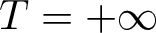 $T=+\infty$) and
 $u(x, \star) \in C^h([0,T])$ for each
 $x \in \Omega$, we will simply write
 $u \in C^k_x(\overline{\Omega}) \cap C^h_t([0,T])$. Finally, in what follows, we use the convention, for the sake of simplicity,
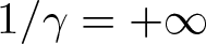 $1/\gamma=+\infty$ when
 $\gamma=0$.
We refer to the beginning of Section 3 for other notations.
We start with some examples which also cover results in [Reference Greco and Kawohl35, Reference Korevaar51, Reference Porru and Serra62] and [Reference Ishige, Salani and Takatsu44].
Theorem 1.1 (Weighted eigenfunctions and logarithmic equations)
Let  $\Omega \subset \mathbb{R}^n$,
 $n\geq 2$, be a bounded, smooth, strongly convex domain. Let
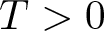 $T \gt 0$,
 $a\colon\Omega\times(0,T]\to \mathbb{R}$,
 $u_0\in C^1(\overline{\Omega})$ with
 $u_0=0$ on
 $\partial\Omega$ and
 $u \in C^2_x(\overline{\Omega}) \cap C^1(\overline{\Omega}\times[0,T])$ be a positive solution of
 \begin{equation*}
\begin{cases}
u_t - \Delta u = a(x,t) f(u) &\quad \hbox{in}\ \Omega \times (0,T], \\
u=0 & \quad\text{on }\partial \Omega\times [0,T], \\
D_x u \cdot \nu \gt 0 & \quad\text{on }\partial \Omega\times [0,T], \\
u =u_0 & \quad \text{on } \overline{\Omega} \times \{0\},
\end{cases}
\end{equation*}
where  $\nu$ is the interior normal to
 $\partial \Omega$. Assume moreover that
 $u_0 \gt 0$ is
 $\log$-concave in
 $\Omega$ and one of the following:
i)
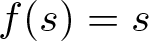
 $f(s)=s$, and $a(\cdot, t)$ is concave for each $t \in (0,T]$;
ii)
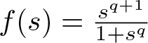
$f(s)=s \log^q(1+s)$ or $f(s)=\frac{s^{q+1}}{1+s^q}$, $q \in (0,1)$, and $a(\cdot,t)$ is $\frac{1}{1-q}$-concave for each $t \in (0,T]$;iii)
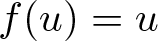
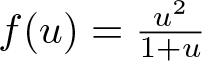
$f(s)=s \log(1+s)$, $f(s)=s \log(s)$ or $f(s)=\frac{s^2}{1+s}$, and $a$ is a positive constant.




Then 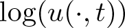 $\log(u(\cdot, t))$ is concave for each
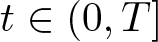
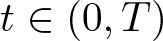 $t \in (0,T)$. Moreover, if
 $a \in C^{2,1}(\Omega\times(0,T])$ and
 $u \in C^{2,1}(\Omega\times(0,T])$, then
 $\log(u(\cdot, t))$ is strictly concave for each
 $t \in (0,T)$; as a consequence, for each
 $t \in (0,T)$ the function
 $u(\cdot, t)$ has a unique, nondegenerate, critical point.
Theorem 1.1 is a particular case of the more general Corollary 5.3; we highlight that the method allows a dependence of  $a$ both in
 $x$ and
 $t$, and to choose
 $a$ sign-changing in point (i) (which allows us to cover a broader range of applicative problems, see also Theorem 1.2 below). Moreover, we highlight the information on strict concavity that we obtain. A generalization of Theorem 1.1 in the sense of perturbed concavity is presented in Theorem 1.5 below and Corollary 5.6. We refer to Remark 2.1 for some technical comments on Theorem 1.1.
As an additional example, we may consider logistic models of population dynamics in heterogeneous environments with lethal boundary. That is, the equation is governed by a logistic law  $b(x,s) = a(x) s - s^2$ where
 $\{a \gt 0\}$ is the favourable habitat while
 $\{a \lt 0\}$ is the hostile one, see [Reference Belgacem and Cosner7, Reference Cantrell and Cosner15, Reference Oruganti, Shi and Shivaji60] (see also Remark 5.10 for bang-bang weights).
Theorem 1.2 (Logistic model)
Let  $\Omega \subset \mathbb{R}^n$,
 $n\geq 2$, be a bounded, smooth, strongly convex domain. Let
 $T \gt 0$,
 $a\colon\Omega\times(0,T]\to \mathbb{R}$,
 $u_0\in C^1(\overline{\Omega})$ with
 $u_0=0$ on
 $\partial\Omega$ and
 $u \in C^2_x(\overline{\Omega}) \cap C^1(\overline{\Omega}\times[0,T])$ be a positive solution of
 \begin{equation*}
\begin{cases}
u_t - \Delta u = a(x,t) u - u^2 &\quad \hbox{in}\ \Omega \times (0,T], \\
u=0 & \quad\text{on }\partial \Omega\times [0,T], \\
D_x u \cdot \nu \gt 0 & \quad\text{on }\partial \Omega\times [0,T], \\
u =u_0 & \quad \text{on } \overline{\Omega} \times \{0\},
\end{cases}
\end{equation*}
where  $\nu$ is the interior normal to
 $\partial \Omega$. Assume moreover that
 $u_0 \gt 0$ is
 $\log$-concave in
 $\Omega$ and
 $a(\cdot,t)$ is concave in
 $\Omega$ for each
 $t\in (0,T]$. Then
 $\log(u(\cdot, t))$ is concave for each
 $t \in (0,T)$. Moreover, if
 $a\in C^{2,1}(\Omega\times(0,T])$ and
 $u \in C^{2,1}(\Omega \times (0,T])$, then
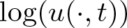 $\log(u(\cdot, t))$ is strictly concave for each
 $t \in (0,T)$.
Compared with [Reference Greco and Kawohl35, Reference Korevaar51, Reference Porru and Serra62], Theorems 1.1 and 1.2 point out some additional models and contain some minor generalizations (e.g. the presence of the weight  $a(x,t)$), which are not substantial but allow us to give a more complete picture. We continue by presenting some examples, inspired by [Reference Kennington48], and which cover models presented in [Reference Ishige and Salani42, Reference Ishige and Salani43].
Theorem 1.3 (Weighted Lane–Emden)
Let  $\Omega \subset \mathbb{R}^n$,
 $n\geq 2$, be a bounded, convex domain which satisfies the interior sphere property.
Let
 $q \in [0,1)$ and
 $\gamma \in [0,1]$. Let
 $u\in C^2_x(\Omega)\cap C^1_x(\overline{\Omega}) \cap C^1_t((0,+\infty)) \cap C(\overline{\Omega}\times[0,+\infty))$ be a positive solution of
 \begin{equation*}
\begin{cases}
u_t-\Delta u=a(x) t^{\gamma} u^q &\quad\text{in }\Omega\times (0,+\infty), \\
u=0 & \quad\text{on }\partial \Omega\times [0,+\infty), \\
u =0 & \quad \text{on } \overline{\Omega} \times \{0\}.
\end{cases}
\end{equation*}
Suppose  $a\colon \Omega \to \mathbb{R}$ to be measurable and that there exists
 $m \gt 0$ such that
 $a(x)\geq m$ for all
 $x\in \Omega$. If
 $\beta \in [1, \frac{1}{\gamma}) \cap [1,2]$ and
 $a$ is
 $\theta$-concave with
 $\theta \geq \frac{1}{1-\beta \gamma}$, then
 $u(\cdot, \star^{\beta})$ is
 $\frac{(1-q)\theta}{2\theta +\beta \gamma \theta+1}$-concave. If
 $\beta \in [1, \min\{\frac{1}{\gamma},2\}]$ and
 $a$ is constant, then
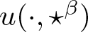 $u(\cdot, \star^{\beta})$ is
 $\frac{1-q}{2+\beta \gamma }$-concave.
We notice that, if  $q=0$, the condition
 $a(x) \geq m \gt 0$ above can be relaxed into
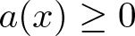 $a(x) \geq 0$, see Proposition 6.5; we highlight in Theorem 1.3 the possibility of the nonlinearity to vanish where
 $u=0$, which is a nontrivial improvement compared to [Reference Kennington48]. Theorem 1.3 is a particular case of the more general Corollary 5.18. We highlight that, whereas [Reference Ishige and Salani43, Theorem 3] and [Reference Ishige and Salani42, Theorem 4.1] rely on a priori assumptions on the solution
 $u$, in Theorem 5.16 and Corollary 5.18 we focus instead on furnishing operative conditions to check on the nonlinearity. Notice that Theorem 1.3 somehow unifies [Reference Ishige and Salani43, Theorem 5 and Theorem 6] (see also [Reference Ishige and Salani42, Theorem 5.3 and Corollary 6.1]), even if such generalization is not deducible from the arguments in [Reference Ishige and Salani42, Reference Ishige and Salani43].
A quantitative version of Theorem 1.3 can be found in Theorem 1.6 below and Corollary 5.17. We refer to Remark 2.2 for more technical comments on Theorem 1.3.
To mention another consequence of our general setting, we propose here the concavity of solutions for nonhomogeneous nonlinearities. Let us mention that our approach allows us to recover also the quasiconcavity obtained by [Reference Kennington48] (see Proposition 5.19 and the subsequent remark), and to treat gradient-type equations (see e.g. Remark 5.5).
Theorem 1.4 (Sum of powers)
Let  $\Omega \subset \mathbb{R}^n$,
 $n\geq 2$, be a bounded, convex domain which satisfies the interior sphere property.
Let
 $q\in (\frac{1}{3},1)$ and
 $p\in (\frac{3q-1}{2},q)$. Let
 $u\in C^2_x(\Omega)\cap C^1_x(\overline{\Omega}) \cap C^1_t((0,+\infty)) \cap C(\overline{\Omega}\times [0,+\infty))$ be a positive solution of
 \begin{equation*}
\begin{cases}
u_t-\Delta u= a(x) u^p+u^q &\quad\text{in }\Omega\times (0,+\infty), \\
u=0 & \quad\text{on }\partial \Omega\times [0,+\infty), \\
u =0 & \quad \text{on } \overline{\Omega} \times \{0\}.
\end{cases}
\end{equation*}
Suppose  $a\colon \Omega \to \mathbb{R}$ to be measurable and that there exists
 $m \gt 0$ such that
 $a(x)\geq m$ for all
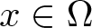 $x\in \Omega$; assume moreover
 $a$ to be
 $\theta$-concave with
 $\theta \in [\frac{1-q}{2(q-p)}, +\infty]$. Then we have that
 $u(\cdot, \star^{2})$ is
 $\frac{1-q}{2}$-concave.
We postpone the discussion of the technical difficulties of Theorems 1.1–1.4 (and of the corresponding generalizations Corollaries 5.3 and 5.18), see Remark 2.4.
As aforementioned, the second and main goal of this paper is to deal with quantitative versions of the concavity maximum principles. Recently, quantitative versions of symmetry results have been considered, for example, in [Reference Amato, Barbato, Masiello and Paoli5, Reference Ciraolo, Cozzi, Perugini and Pollastro21, Reference Dipierro, da Silva, Poggesi and Valdinoci29, Reference Gatti33]; we also mention [Reference Ciraolo, Figalli and Maggi22, Reference Deng, Sun and Wei27] where the error from bubble functions is quantified in Sobolev critical equations. In the realm of concavity properties, instead, similar results have been recently investigated in the elliptic case in [Reference Bucur and Squassina13] (see also [Reference Almousa, Bucur, Cornale and Squassina3, Reference Gallo and Squassina32]); such estimates are made in terms of some parameter of the weight  $a(x)$: more precisely, in these papers the authors show that, if
 $a$ is close to a constant function, then some power of
 $u$ is close to a concave function, up to some explicit error. We also mention the recent [Reference Hamel and Nadirashvili36] where a concavity result is obtained for problems with small perturbations, by exploiting the strong
 $\log$-concavity of the eigenfunction.
In this paper, we deal with estimations of the (space) concavity function of a solution  $v$ (see (3.5))
 \begin{equation*} \mathcal{C}^*_v(x_1,x_3,\lambda, t) :=v(x_2, t)-\lambda v(x_3, t)-(1-\lambda)v(x_1,t), \end{equation*}
or the (spacetime) concavity function
 \begin{equation*}\mathcal{C}_v(x_1,x_3,t_1,t_3,\lambda):= v(x_2,t_2)-\lambda v(x_3,t_3)-(1-\lambda)v(x_1,t_1),\end{equation*}
where  $x_1, x_3 \in \Omega $,
 $t_1, t_3 \in [0,+\infty)$,
 $\lambda \in [0,1]$ and
 $x_2=\lambda x_3+(1-\lambda)x_1$ and
 $t_2=\lambda t_3+(1-\lambda)t_1$; notice that
 $\mathcal{C}_v \geq 0$ if and only if
 $v$ is concave. Our goal is, as already anticipated, to generalize the abovementioned results also to the parabolic setting, which seems to be new in the literature. As a consequence of our general results, we get in particular the following statement. Here
 $f^- := \max\{0,-f\}$ stands for the negative part of a function
 $f$, while
 ${\rm osc}(a):= \sup(a) - \inf(a)$ stands for the oscillation of
 $a$.
Theorem 1.5 (Quantitative concavity, I)
Let  $\Omega \subset \mathbb{R}^n$,
 $n\geq 2$, be a bounded, smooth, strongly convex domain. Let
 $T \gt 0$,
 $a\colon \Omega \times (0,T] \to \mathbb{R}$ bounded,
 $u_0\in C^1(\overline{\Omega})$ with
 $u_0=0$ on
 $\partial\Omega$ and
 $u \in C^2_x(\Omega) \cap C^1(\overline{\Omega}\times[0,T])$ be a positive solution of
 \begin{equation*}
\begin{cases}
u_t - \Delta u = a(x,t) u &\quad \hbox{in}\ \Omega \times (0,T], \\
u=0 & \quad\text{on }\partial \Omega\times [0,T], \\
D_x u \cdot \nu \gt 0 & \quad\text{on }\partial \Omega\times [0,T], \\
u =u_0 & \quad \text{on } \overline{\Omega} \times \{0\},
\end{cases}
\end{equation*}
where  $\nu$ is the interior normal to
 $\partial \Omega$. Assume moreover that
 $u_0 \gt 0$ is
 $\log$-concave in
 $\Omega$. Then
 \begin{equation*}\inf_{\Omega \times \Omega \times [0,1] \times [0,T]} \mathcal{C}^*_{\log(u)} \geq -e T \sup_{\Omega \times \Omega \times [0,1] \times (0,T]} \left(\mathcal{C}^*_{a(\cdot, \star)}\right)^-.\end{equation*}
In Theorem 1.5, one may also consider other nonlinearities, like the ones in Theorem 1.1 (see Corollary 5.6). Moreover, if  $u_0$ is not assumed to be
 $\log$-concave, then an additional error related to
 $\mathcal{C}_{\log(u_0)}$ appears (see Remark 5.2).
Theorem 1.6 (Quantitative concavity, II)
Let  $\Omega \subset \mathbb{R}^n$,
 $n\geq 2$, be a bounded, convex domain which satisfies the interior sphere property. Let
 $q \in [0,1)$. Let
 $u\in C^2_x(\Omega)\cap C^1_x(\overline{\Omega}) \cap C^1_t((0,+\infty)) \cap C(\overline{\Omega}\times [0,+\infty))$ be a positive solution of
 \begin{equation*}
\begin{cases}
u_t-\Delta u=a(x) u^q &\quad\text{in }\Omega\times (0,+\infty), \\
u=0 & \quad\text{on }\partial \Omega\times [0,+\infty), \\
u =0 & \quad \text{on } \overline{\Omega} \times \{0\}.
\end{cases}
\end{equation*}
Suppose  $a\colon\Omega \to \mathbb{R}$ to be measurable and
 $0 \lt m \leq a \leq M$. Then
 $u$ is increasing in time and
 \begin{equation}
\min_{\overline{\Omega}\times \overline{\Omega}\times[0,+\infty]\times [0,+\infty]\times[0,1]}\mathcal{C}_{u^{\frac{1-q}{2}}} \geq
- \|u(\cdot, \infty)\|_{L^{\infty}(\Omega)}^{\frac{1-q}{2}} \frac{{\rm osc}(a^2)}{m^2},
\end{equation}
where  $u(\cdot, \infty)$ is the solution of the corresponding stationary problem.
If moreover  $\theta \geq 1$ and
 $m^\theta\geq M^{\theta}/2$, then
 \begin{equation}
\min_{\overline{\Omega}\times \overline{\Omega}\times[0,+\infty]\times [0,+\infty]\times[0,1]}\mathcal{C}_{u^{\frac{\theta(1-q)}{2\theta+1}}}
\geq
-\frac{\theta }{\theta+1} \frac{1}{m} \|u(\cdot, \infty)\|_{L^{\infty}(\Omega)}^{\frac{\theta(1-q)}{2\theta+1}}
\sup\limits_{\Omega \times \Omega\times[0,1]}
(\mathcal{C}^-_{a^{\theta}})^{1/\theta}.
\end{equation}
We refer to Remark 2.3 for some additional comments. We highlight that estimate (1.1) in Theorem 1.6 is slightly finer if compared with the ones obtained in the elliptic setting in [Reference Bucur and Squassina13, Reference Gallo and Squassina32]. Moreover, the estimate (1.2) does not involve the oscillation of  $a$ and is totally new, even for the elliptic setting. Indeed, some results of this paper can be easily adapted to the elliptic framework, allowing us to improve and generalize some previous results [Reference Bucur and Squassina13, Reference Gallo and Squassina32]. By way of example, with the same techniques, we obtain the following statement. We leave the details to the interested reader.
Theorem 1.7 ($\theta$-concavity estimate)

Let  $\Omega \subset \mathbb{R}^n$,
 $n\geq 2$, be a bounded, convex domain which satisfies the interior sphere property, and let
 $q \in [0,1)$. Let
 $u\in C^2(\Omega)\cap C^1(\overline{\Omega})$ be a positive solution of
 \begin{equation*}\begin{cases}
-\Delta u = a(x) u^q & \quad \hbox{in}\ \Omega, \\
u=0 & \quad \hbox{on}\ \partial \Omega.
\end{cases}
\end{equation*}
Suppose  $a\colon \Omega \to \mathbb{R}$ to be measurable and
 $0 \lt m\leq a \leq M$ and
 $1\leq\theta \leq\log(2)/\log(\frac{M}{m})$. Then
 \begin{equation*} \min_{\overline{\Omega}\times \overline{\Omega}\times[0,1]}\mathcal{C}_{u^{\frac{\theta(1-q)}{1+2\theta}}}
\geq
-\frac{\theta}{1+\theta} \frac{1}{m}||u||_\infty^{\frac{\theta(1-q)}{1+2\theta}}
\sup\limits_{\Omega \times \Omega\times[0,1]}
(\mathcal{C}^-_{a^{\theta}})^{1/\theta}.
\end{equation*}
As already mentioned, the main tool of this paper is composed by concavity and harmonic concavity maximum principles, which allow us to give an estimate on the concavity function  $\mathcal{C}_v$ of a solution of a general PDE in terms of the concavity/harmonic concavity function of the nonlinear term (see Definition 3.7). The equations treated do not rely on the boundary conditions and can have a very general form (see Theorems 4.1, 4.4), and in particular include the equations satisfied by
 $v=\log(u)$ or
 $v=u^{\alpha}$,
 $\alpha \in (0,1)$, where
 $u$ is the solution of the equation of interest. We highlight that the concavity principle approach is flexible since it can be used, for example, to deal with weak solutions of quasilinear equations, see [Reference Borrelli, Mosconi and Squassina11, Reference Gallo and Squassina32, Reference Lin57] (see also Remark 5.10 for another nonsmooth setting), and thus possibly useful for treating
 $p$-Laplace parabolic equations.
We refer to Remark 2.4 for some technical comments on the proofs and corresponding difficulties and novelties.
The paper is organized as follows. In Section 2, we collect some remarks on the main theorems and on the proofs, while in Section 3, we recall some basic facts on parabolic equations, and we introduce the main assumptions that we will require on the nonlinearity. Moreover, we recall notations and properties about concavity functions; more technical results are instead collected in Appendix B. Section 4 is devoted to the proof of the main concavity principles, which take into account only the PDE and not the boundary/initial conditions; these theorems will lead both to exact and quantitative results. In particular, we show both concavity principles in space (in the presence of nonlinearities which are concave but not necessarily decreasing, and set in  $(0,T]$) and in space-time (in the case of harmonic concave and decreasing nonlinearities set in
 $(0,+\infty)$); the latter will require the use of the harmonic concavity function. In Section 5, we take into account the boundary conditions and the initial condition, employing a suitable analysis of the solution and of the concavity function near the boundary of the parabolic cylinder; this analysis also exploits comparison principles and Hopf lemmas, which are collected in Appendix A. Some applications and examples follow, including the proofs of the main theorems presented in the introduction. When the nonlinearity does not depend on
 $u$, finally, we present some further results (both simplifications and improvements of the previous ones) in Section 6.
2. Some remarks on the theorems
We collect in this section some technical comments on the main theorems and on the proofs and difficulties of the present paper.
Remark 2.1 (On Theorems 1.1 and 1.2)
We observe the following facts.
• Once concavity is obtained, the strict concavity of solutions is usually gained, in elliptic PDEs, through the use of a constant rank theorem. Parabolic versions of the constant rank theorem have been obtained in a space version in [Reference Bian and Guan8, Reference Caffarelli, Guan and Ma14], and in a spacetime version in [Reference Chen18, Reference Chen and Hu19] (see Proposition 3.11). We mention that, in our case, the conclusion for the weighted eigenfunction (case (i)) can be obtained in a more straightforward way by assuming
$a$ strictly concave in $x$ (and no additional regularity), see Remark 5.4; similar properties appear in [Reference Bitterlin10] in the setting of periodic solutions.• The condition
$D_x u \cdot \nu \gt 0$ already appears in the papers [Reference Greco and Kawohl35, Reference Korevaar51]; we point out the requirement also in $t=0$ (that is, $u_0 \in C^1(\overline{\Omega})$ and $D_x u_0 \cdot \nu \gt 0$) which, as highlighted in [Reference Greco and Kawohl35, Section 6], is essential but erroneously neglected in previous papers; in the same section, the authors provide an approximation process in order to avoid this restriction in zero (in particular, allowing $u_0 \in C(\overline{\Omega})$). Moreover, in [Reference Greco and Kawohl35, Remark 2, page 7] the authors comment on the validity of such condition for general classes of nonlinearities. For example, assume $a \geq 0$ and $D_x u_0 \cdot \nu \gt 0$. Then $f(s) \geq 0$ is sufficient to ensure this condition thanks to the parabolic Hopf Lemma A.4; this covers almost every case of Theorem 1.1. To treat $f(s)=s \log(s)$, assuming moreover $M \geq a \geq m \gt 0$, we see that it is sufficient to choose $u_0$ such that $u_0 \geq w$ where $w$ is a positive solution to the stationary problem $-\Delta w = f(w)$ which, by [Reference Vázquez65, Theorem 2] verifies $D_x w \cdot \nu \gt 0$; then a comparison principle and $u=w=0$ on $\partial \Omega$ imply $D_x u \cdot \nu \geq D_x w \cdot \nu \gt 0$.• The requirement on the smoothness of
$\Omega$ (not required in Theorem 1.3 below) is here related to the control of the concavity function of $\log(u)$ near the boundary, by means of the positivity of the curvatures. Anyway, this condition can be relaxed through some standard approximation of the domain $\Omega$, see e.g. [Reference Borrelli, Mosconi and Squassina11, Reference Gallo and Squassina32].• We highlight that the logarithmic equation
$f(s)=s \log(s)$, being superlinear and sign-changing, is a problem not easy to tackle in the elliptic framework, see [Reference Gallo, Mosconi and Squassina31]; in the parabolic framework, on the other hand, it can be addressed through a suitable drift in time (see (4.5)). Notice moreover that the result is obtained on $[0,T]$ and, generally, the solutions of this problem do not converge to the one of the stationary problem (see Remark 5.7), thus it is not straightforward to obtain the elliptic result from the parabolic one.


Remark 2.2 (On Theorems 1.3 and 1.4)
We observe the following facts.
• We see that the exponent
$\alpha=\frac{(1-q)\theta}{2\theta +\beta \gamma \theta+1}$ is consistent with the results in [Reference Gallo and Squassina32, Reference Kennington49], where $\alpha=\frac{(1-q)\theta}{2\theta+1}$ if the problem is elliptic (and thus $\gamma=0$), and in [Reference Ishige and Salani42, Reference Ishige and Salani43], where $\alpha = \frac{\theta}{2\theta+\beta\gamma \theta+1}$ if the nonlinearity does not depend on $u$ (i.e. $q=0$).• The initial condition
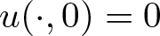
$u(\cdot, 0)=0$ also appears in [Reference Ishige and Salani42, Reference Ishige and Salani43, Reference Kennington48], and we mention that, for such a sublinear problem, nontrivial solutions generally may exist (see Remark 3.1). See also Remark 5.26 for some comments on the case $u(\cdot, 0)\neq 0$.• If
$u$ is nondecreasing in time (and this is the case of our setting, see Theorem 5.16), then if $u(\cdot,\star^{\beta_1})$ is $\alpha$-concave then $u(\cdot,\star^{\beta_2})$ is $\alpha$-concave for all $\beta_2\leq \beta_1$, see [Reference Ishige and Salani43, Section 2, Property (e)] (see also (3.7)).




Remark 2.3 (On Theorems 1.5 and 1.6)
We observe the following facts.
• In Theorem 1.6 we observe that
$ \|u(\cdot, \infty)\|_{L^{\infty}(\Omega)}$ could be bounded in terms of known quantities of the problems, i.e. $n$, $|\Omega|$, $q$, $m$ and $M$, see e.g. [Reference Ciraolo, Cozzi, Perugini and Pollastro21, proof of Corollary 1.4(b)].• In Theorem 1.6 the condition
$m^\theta\geq M^{\theta}/2$ comes into play in showing quantitative concavity properties of products (see Proposition B.1), but we believe it is technical.


Remark 2.4 (On the proofs)
As mentioned in the introduction, differently from [Reference Ishige and Salani42–Reference Ishige, Salani and Takatsu44], our proofs rely on concavity maximum principles, which also allow us to keep track of the concavity error. Such maximum principles require that the minimum of the concavity function is in the interior of the domain: to ensure such a property, we will exploit both the information at the boundary  $\partial \Omega\times [0,+\infty)$ and the information at
 $\Omega \times \{0\}$; when treating equations in
 $(0,+\infty)$, we will also exploit the information on the stationary problem (i.e.
 $t=+\infty$) (see Section 5.2). When
 $a(x,t)$ depends on
 $t$ in a coercive way (for instance,
 $a(x,t)=a(x) t^{\gamma}$) we also implement a truncation argument in order to be able to compare the problem with a stationary one at infinity (see Remark 3.6). In such a way, we control all the information on
 $\partial(\Omega \times (0,+\infty))$ and we can apply the concavity maximum principles. We notice that, when dealing with
 $T \lt +\infty$, the nonlinearity is concave and concavity is discussed only in the spatial sense, no a priori information on
 $u$ in
 $t=T$ is needed. To further treat equations like the logarithmic one, we need to implement a correction in time of the type
 $e^{\mu t}$,
 $\mu$ large, which allows us to decrease the monotonicity in
 $u$ of the nonlinearity involved, recovering the nonincreasing monotonicity which is needed for the argument (see (4.5), (4.3) and (4.7) in Theorem 4.1).
To gain the above results, we make some technical assumptions: on the nonlinearity  $b(x,s,t)$ we require some conditions to ensure that
 $u(x, \cdot)$ is monotone nondecreasing, and it converges to the stationary problems (see conditions (H2), (H3) and (i)–(iv) in Remark 3.3). Moreover, we need to ensure the validity of some comparison principles (notice that
 $b(x,\cdot,t)$, in this setting, cannot be generally assumed locally Lipschitz) and that
 $u$ can be compared through such a tool with some suitable known subsolution, whose behaviour near
 $t=0$ and near
 $\partial \Omega$ is known (see conditions (H1)-(H2)); in particular we highlight that, compared with [Reference Kennington48], the nonlinearities of interest in this paper vanish at zero, thus a finer analysis is needed. We notice again that, when logarithmic transformations are considered and the concavity is discussed only in the spatial sense, then the analysis on the boundary essentially relies on the strong convexity of the domain. Finally, in order to adapt the above proofs to some quantitative version and keep track of all the interested quantities in play, a finer and technical analysis of the relations among concavity and harmonic concavity functions is needed (see Appendix B).
3. Preliminaries
In what follows, we will denote by  $\Omega \subset \mathbb{R}^n$ an open, bounded, and convex domain. By smooth, we will mean
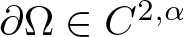 $\partial\Omega\in C^{2,\alpha}$, while by strongly convex we will mean that the second fundamental form with respect to its interior normal is positive definite everywhere. We moreover recall that
 $\Omega$ satisfies the interior sphere condition if for all
 $x\in \partial \Omega$, there exist
 $y\in \Omega$ and
 $r \gt 0$ such that
 $B_r(y)\subseteq \Omega$ and
 $x\in \partial B_r(y)$. We set
 $ d_\Omega(x):= \text{dist}(x,\partial \Omega)$ and
 \begin{equation*}\Omega_\rho:=\left\{x\in \Omega: d_{\Omega}(x) \gt \rho\right\}\end{equation*}
for  $\rho \gt 0$. We also denote
 $f^+:=\max\{0,f\}$ and
 $f^-:=\max\{0, -f\}$ the positive and negative parts of a function
 $f\colon \Omega \to \mathbb{R}$, so that
 $f=f^+-f^-$, and by
 \begin{equation*}{\rm osc}(f):=\sup_{\Omega} f-\inf_{\Omega} f\end{equation*}
the oscillation of  $f$, whenever well defined.
In the whole paper,  $\cdot$ represents spatial dependence and
 $\star$ time dependence, e.g. we write
 $u(\cdot, \star)$ for
 $u\colon \overline{\Omega} \times [0,T] \to \mathbb{R}$.
We finally denote
 \begin{equation*}Du:=(D_x u,\partial_t u) =(D_x u, u_t)\end{equation*}
where  $D_x$ is the spatial gradient and
 $\partial_t$ is the time derivative of
 $u$; in this regard, we will often decompose vectors as
 $p=(\tilde{p}, p^{n+1}) \in \mathbb{R}^n \times \mathbb{R} = \mathbb{R}^{n+1} $.
3.1. On parabolic equations
In this subsection, we recall some facts on the parabolic problem
 \begin{equation}
\begin{cases}
u_t-\Delta u=b(x,u,Du, t) &\text{in }\Omega\times (0,+\infty),\\
u \gt 0 & \text{in } \Omega\times (0,+\infty),\\
u=0 & \text{on }\partial \Omega\times (0,+\infty),\\
u=u_0& \text{on } \Omega \times \{0\},
\end{cases}
\end{equation}
where  $b\colon\Omega\times \mathbb{R}\times \mathbb{R}^{n+1}\times \mathbb{R}\to \mathbb{R}$.
Remark 3.1. We briefly comment on existence and regularity results for problem (3.1) when  $b(x,s,p,t)=a(x) f(s)$ and
 $u_0=0$. Assumed
 $a\in C(\overline{\Omega})\cap C^\sigma(\Omega)$,
 $\sigma \in (0,1]$,
 $a\not\equiv 0,$
 $a\geq 0$,
 $f\in C([0,+\infty))$, nondecreasing,
 $f(0)=0$ and
 $f \gt 0$ on
 $(0,+\infty)$ we have that (3.1) admits a nontrivial solution if (and only if) (see [Reference Fujita and Watanabe30, Theorem 1.5], [Reference Laister, Robinson and Sierżęga53, Corollary 2.6])
 \begin{equation*} \int_{0}^{\varepsilon}\frac{1}{f(s)}ds \lt +\infty \quad\text{for some }\varepsilon \gt 0.\end{equation*}
Observe that  $f(s)= s^q$ with
 $q\in [0,1)$ satisfies such condition. For regularity results, we refer again to [Reference Fujita and Watanabe30, Reference Laister, Robinson and Sierżęga53]. For local and global existence in the case
 $u_0 \neq 0$, see e.g. [Reference Kajikiya47, Lemma 3.5 and Theorem 2.1]. We further mention the existence of weighted eigenfunctions with periodic conditions, see [Reference Daners25, Reference Godoy and Kaufmann34] and references therein; see also Remark 5.7 for some comments on the logarithmic equation.
To give concavity information on the boundary of  $(0,+\infty)$, and in particular for
 $t=+\infty$, we need to be able to compare the evolutive problem with the stationary one. We thus give the following definition.
Definition 3.2. Let  $\Omega \subset \mathbb{R}^n$ be open and consider
 $u\colon\Omega\times (0,+\infty)\to \mathbb{R}$ such that (3.1) holds. We will say that
 $b$ satisfies the parabolic stability condition if
 \begin{equation}
\lim\limits_{t\to +\infty} ||u(\cdot,t)-v||_{L^\infty(\Omega)}=0
\end{equation}
for some  $v\colon\Omega\to \mathbb{R}$ solution of
 \begin{equation}
\begin{cases}
-\Delta v=b(x,v,D_xv,\infty) &\textrm{in }\Omega,\\
v=0 & \textrm{on }\ \partial \Omega;
\end{cases}
\end{equation}
here  $b(x,s,\tilde{p},\infty):=\lim\limits_{t\to+\infty}b(x,s,\tilde{p}, 0,
t)$ is assumed to exist for all
 $(x,s,p)\in \Omega\times (0,+\infty)\times \mathbb{R}^{n+1}$, where
 $p=(\tilde{p},p^{n+1})$.
Remark 3.3. We briefly comment on the validity of the parabolic stability condition: in [Reference Akagi and Kajikiya1, Theorem 1.1] it is proved that such property is satisfied by the power  $b(x,s,p,t)=|s|^{q-1}s$ where
 $0 \lt q \lt 1$.
Other examples can be deduced by [Reference Kajikiya47]: suppose indeed that
 $b(x,s,p,t)=b(x,s)$ satisfies the following facts
i)
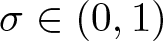
$b \in C(\overline{\Omega}\times \mathbb{R}) \cap C_{loc, x}^{\sigma}(\mathbb{R})$ for some $\sigma\in (0,1)$ and $b(x, \cdot)$ is odd for each $x \in \Omega$;ii) there exists
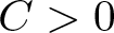
$C \gt 0$ such that
where\begin{equation*} |b(x,s)|\leq C(|s|^q+1)\quad \text{for }s\in\mathbb{R}, \ x\in \overline{\Omega} ,\end{equation*}$q \gt 1$ if $n=1,2$ and $q\in (1,\frac{n}{n-2})$ if $n\geq 3$;iii) it holds
where\begin{equation*} \limsup_{|s|\to +\infty} \left(\max_{x\in \overline{\Omega}}\frac{b(x,s)}{s}\right) \lt \lambda_1,\end{equation*}$\lambda_1$ is the first eigenvalue of the Laplacian.





Then, for any  $u_0 \in H^1_0(\Omega)$, [Reference Kajikiya47, Theorem 2.1] states that the orbit of
 $u(\cdot,t)$ for all
 $t\in(0,+\infty)$ is relatively compact in
 $C^{1,\theta}(\overline{\Omega})$ for some
 $\theta\in (0,1)$, and the limit points are stationary solutions. Suppose moreover that
iv)
$s\in(0,+\infty) \mapsto \frac{b(x, s)}{s}$ is strictly decreasing for each $x \in \Omega$


so that the limit problem (3.3) admits a unique solution  $v$ by a Brezis–Oswald result (see e.g. [Reference Gallo and Squassina32, Lemma A.1]), then
 $u(\cdot,t) \to v $ in
 $C^{1,\theta}(\overline{\Omega})$, which in particular implies (3.2). Notice that, if (i) and (iv) hold, then (iii) means
 $\inf_{s \gt 0} \left(\max_{x\in \overline{\Omega}}\frac{b(x,s)}{s}\right) \lt \lambda_1$. We are confident that the relative compactness to stationary solutions — which is weaker than the parabolic stability condition, and does not require (iv) — is sufficient to prove Theorem 5.16. On the other hand, in order to make use of the notation
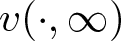 $v(\cdot,\infty)$ and keep the presentation simple, we prefer not to improve the generality of the result.
Some functions that satisfy (i)–(iv) are given by  $b(x,s)=a(x) f(s)$ with
 $f(s)=|s|^{q-1}s$ or
 $f(s)=-s\log |s|$, and
 $a \in C(\overline{\Omega})$ is positive. Moreover, the sum of these functions also satisfies (i)–(iv). The nonlinearity
 $b(s)=(1-s)^q$,
 $q \in (0,1)$ (see [Reference Kennington48]), does not verify
 $(i)$, but nevertheless verifies the parabolic stability condition when
 $u_0=0$: this can be shown in a standard way, once observed that
 $0\le u(x,t)\le v(x) \leq \|v\|_{L^\infty(\Omega)} \lt 1$, where
 $v$ is the unique positive stationary solution, that
 $u_t \geq 0$ by Corollary A.3, and that standard parabolic estimates hold.
Our problems will often involve a nonlinear term  $b=b(x,s,t)$; we present here some main assumptions for
 $b\colon\Omega\times(0,+\infty) \times (0,+\infty)\to \mathbb{R}$.
There exists  $T \gt 0$,
 $M \gt 0$,
 $k \gt 0$,
 $q\in [0,1)$, and
 $\gamma \in [0,1]$, such that
 \begin{equation*}b(x,s, t)\geq k t^{\gamma} s^q \quad \hbox{for all}\ (x,s,t)\in \Omega\times(0,M]\times (0,T].\end{equation*}
There exists  $T \gt 0$ such that
 $b(\cdot,s,t)$ is measurable and nonnegative for
 $(s,t)\in(0,+\infty)\times (0,T)$, and for all
 $M \gt 0$ there exists
 $L=L(M,T) \gt 0$ verifying
 \begin{equation*}b(x,s,t)-b(x,r,t)\leq \frac{L}{r}(s-r) \quad \hbox{for all}\ 0 \lt r\leq s\leq M\ \text{and}\ (x,t) \in \Omega \times (0, T].\end{equation*}
The function  $b(x,s,\cdot)$ is nondecreasing for each
 $(x,s) \in \Omega \times (0,+\infty)$.
With no loss of generality, whenever assumed together, we can choose the constant  $T$ in (H1)-(H2) to be the same. In practical situations, the constant
 $M$ in (H2) will actually be given by the
 $L^\infty$-norm of the solution involved. Moreover, since we will apply (H1) only for small values of
 $t$, if
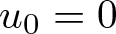 $u_0=0$ then for
 $t$ small
 $\|u(\cdot, t)\|_{L^{\infty}(\Omega)}$ can be chosen to be smaller than the fixed
 $M$ in (H1) (see also condition (H1*)).
Remark 3.4. Observe that the function  $b(x,s,t) = a(x,t) s^q$, with
 $q \in (0,1)$ and
 $a \in L^{\infty}(\Omega \times \mathbb{R})$ nonnegative, satisfies (H2). Indeed, for each
 $0 \lt r\leq s\leq M$ by Lagrange theorem there exists
 $\xi\in (r,s)$ such that
 \begin{align*}
b(x,s,t) - b(x,r,t) = a(x, t) \frac{q}{\xi^{1-q}}(s-r)\leq \|a\|_{\infty} \frac{q s^q}{r}(s-r)\leq \|a\|_{\infty} \frac{q M^q}{r}(s-r).
\end{align*}
Notice finally that (H2) is closed under summation.
Remark 3.5. In our arguments, it is possible to substitute (H2) with the following:
There exists 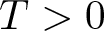 $T \gt 0$ and
 $\omega \in [\frac{1}{2},1]$ such that
 $b(\cdot,s,t)$ is measurable and nonnegative for
 $(s,t)\in(0,+\infty)\times (0,T)$, and for all
 $M \gt 0$ there exists
 $ L=L(M,T) \gt 0$ verifying
 \begin{equation*} b(x,s,t)-b(x,r,t)\leq L (s-r)^{\omega} \quad \hbox{for all}\ 0 \lt r\leq s\leq M, x\in \Omega\ \text{and}\ t\in (0,T).\end{equation*}
Notice that any  $\omega$-Hölder function with
 $\omega \in [\frac{1}{2},1]$ satisfies (H2*); moreover
 $b(s)=\sqrt{s |1-s|}$ satisfies (H2*) but not (H2). On the other hand, from a practical point of view related to the applications in the present paper, we see that (H2*) is somehow stronger than (H2), since
 $b(s)=s^q$ with
 $q\in (0,\frac{1}{2})$ satisfies (H2) but not (H2*). See also Remark 5.26.
Remark 3.6. We see that fixed  $T \gt 0$ and set
 \begin{equation*}b_T(x,s,t):=
\begin{cases}
b(x,s,t) & \quad \hbox{for}\ t \in [0,T], \\
b(x,s,T) & \quad \hbox{for}\ t \in [T,+\infty),
\end{cases}
\end{equation*}
then, if  $b$ satisfies (H2) (resp. (H3)), then
 $b_T$ satisfies (H2) (resp. (H3)) as well. As a consequence of the uniqueness result in Proposition A.1, since
 $b$ and
 $b_T$ coincide for
 $t \in [0,T]$, we see that positive solutions of
 \begin{equation*}
\begin{cases}
u_t-\Delta u = b(x,u,t)&\hbox{in }\Omega\times(0,+\infty),\\
u=0 &\hbox{on } \partial \Omega\times(0,\infty),\\
u=u_0&\hbox{on }
\Omega \times \{0\},
\end{cases}
\quad
\begin{cases}
v_t-\Delta v = b_T(x,v,t)&\hbox{in }\Omega\times(0,+\infty),\\
v=0 &\hbox{on } \partial \Omega\times(0,\infty),\\
v=u_0&\hbox{on }
\Omega \times \{0\},
\end{cases}
\end{equation*}
coincide on  $[0,T]$. As a consequence, to study (exact) concavity of the first equation, we can study concavity of the second one and obtain the result thanks to the arbitrariness of
 $T$. Notice that the second problem has the advantage of possibly satisfying the parabolic stability condition even if
 $b(x,s,t) \to +\infty$ as
 $t\to +\infty$ (for instance,
 $b(x,s,t)=t^{\gamma} a(x) s^q$). Indeed, consider
 $v$ solution of the second system and define
 $\tilde{v}(x,t):=v(x,t+T)$. Then
 $\tilde{v}$ satisfies
 \begin{equation*}
\begin{cases}
\tilde{v}_t-\Delta \tilde{v} = b_T(x,\tilde{v},t+T) = b(x, \tilde{v}, T) &\hbox{in }\Omega\times(0,+\infty),\\
\tilde{v}=0 &\hbox{on } \partial \Omega\times(0,\infty),\\
\tilde{v}=v(T) \in H^1_0(\Omega) &\hbox{on }
\Omega \times \{0\}.
\end{cases}
\end{equation*}
Thus, if  $b(x,s,T)$ satisfies the parabolic stability condition and
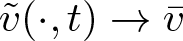 $\tilde{v}(\cdot, t) \to \bar{v}$ uniformly,
 $\bar{v}$ solution of a stationary problem
 $-\Delta \bar{v} = b(x,\bar{v}, T)$, then
 $v(\cdot,t)\to \bar{v}$ uniformly as well, and thus
 $b_T(x,s,t)$ satisfies the parabolic stability condition as well.
3.2. Power concavity and concavity functions
Let us recall some notions about  $\alpha$-concavity, see [Reference Kennington49] for details.
Notation. Throughout the paper, whenever  $z_1, z_3$ are picked in a convex domain together with a
 $\lambda \in [0,1]$, we will denote by
 $z_2$ the convex combination
 \begin{equation*}z_2 \equiv \lambda z_3 + (1-\lambda) z_1.\end{equation*}
Moreover, whenever a function  $g$ is in play, we will denote
 \begin{equation*}g_i \equiv g(z_i) \quad \hbox{for}\ i=1,2,3,\end{equation*}
if it creates no ambiguity. Finally if  $x\in \mathbb{R}^n$, then
 $x^i$ denotes the
 $i$-th component of
 $x$.
Let  $\alpha \in [-\infty, +\infty]$. We recall that a nonnegative function
 $u\colon\Omega \to \mathbb{R}$ is
 $\alpha$-concave if
 \begin{equation}
\begin{cases}
u \text{ is constant} & \text{if } \alpha =+\infty,\\
u^\alpha \text{ is concave} & \text{if } 0 \lt \alpha \lt +\infty,\\
\log(u) \text{ is concave} & \text{if } \alpha =0,\\
u^\alpha \text{ is convex} & \text{if } -\infty \lt \alpha \lt 0,\\
\left\{x\in \Omega: u(x) \gt t\right\} \text{ is
convex }\forall t\in \mathbb{R} & \text{if }\alpha=-\infty;
\end{cases}
\end{equation}
if  $-\infty \lt \alpha\leq 0$ we additionally require
 $u \gt 0$. Moreover, we say that
 $u$ is log-concave if it is
 $0$-concave and quasi-concave if it is
 $(-\infty)$-concave.
With the aim of treating perturbations of concavity, we introduce two operators which allow us to quantify the concavity of a function.
Definition 3.7. Let  $u\colon\Omega\times (0,+\infty) \to \mathbb{R}$, then for each
 $x_1,x_3\in \Omega, \ t_1, \ t_3\in (0,+\infty)$ and
 $\lambda \in [0,1]$, the concavity function
 $\mathcal{C}_u$ is defined as
 \begin{equation}
\mathcal{C}_u(x_1,x_3,t_1,t_3,\lambda):= u(x_2,t_2)-\lambda u(x_3,t_3)-(1-\lambda)u(x_1,t_1)
\end{equation}
where we recall  $x_2=\lambda x_3+(1-\lambda)x_1$ and
 $t_2=\lambda t_3+(1-\lambda)t_1$.
Let  $g\colon\Omega\times (0,+\infty)\to \mathbb{R}$, then we introduce
 \begin{align*}
{\rm Dom}(\mathcal{HC}_g)&:= \Big\{(x_1,x_3,s_1,s_3,\lambda) \in \Omega\times\Omega\times(0,+\infty)\times(0,+\infty)\times[0,1] \mid \\
& \qquad \lambda g(x_1,s_1)+(1-\lambda)g(x_3,s_3) \gt 0 \quad \hbox{or} \quad g(x_1,s_1)=g(x_3,s_3)=0\Big\}
\end{align*}
and the harmonic concavity function  $\mathcal{HC}_g$ defined on
 ${\rm Dom}(\mathcal{HC}_g)$ by
 \begin{equation*}
\mathcal{HC}_g\big((x_1,s_1),(x_3,s_3),\lambda\big):=
\begin{cases}
{g(x_2,s_2)-\dfrac{g(x_1,s_1)g(x_3,s_3)}{\lambda g(x_1,s_1)+(1-\lambda)g(x_3,s_3)}} \\[1ex]
\quad\quad\qquad\qquad\textrm{if } \lambda g(x_1,s_1)+(1-\lambda)g(x_3,s_3) \gt 0,
\\[1ex]
g(x_2,s_2)
\qquad\textrm{if }
g(x_1,s_1)=g(x_3,s_3)=0.
\end{cases}
\end{equation*}
We say that  $g$ is harmonic concave if
 $\mathcal{HC}_g \geq 0$ on its domain. Notice that, if
 $g \geq 0$, then
 ${\rm Dom}(\mathcal{HC}_g)=\Omega\times\Omega\times(0,+\infty)\times(0,+\infty)\times[0,1]$; moreover, if
 $f\geq g$, then
 ${\rm Dom}(\mathcal{HC}_g) \subseteq {\rm Dom}(\mathcal{HC}_f)$. Finally, if
 $g \gt 0$, then the harmonic concavity is equivalent to the
 $(-1)$-concavity in (3.4), while if
 $g \lt 0$ then
 $g$ is always harmonic concave being
 ${\rm Dom}(\mathcal{HC}_g)=\emptyset$.
Remark 3.8. In the rest of the paper, we will implicitly assume that the computations involving  $\mathcal{HC}_g$ are made in the points of its domain.
We have [Reference Bucur and Squassina13, page 4]
 \begin{equation}
\mathcal{HC}_g \geq \mathcal{C}_g,
\end{equation}
and, for any  $\beta \in (0,1]$, (see [Reference Ishige and Salani43, equation (2.2)])
 \begin{equation}
\mathcal{HC}_{u(\cdot, \star^{\beta})}(x_1, x_3, t_1,t_3,\lambda) \geq \mathcal{HC}_{u(\cdot, \star)}(x_1, x_3,t_1^{\beta},t_3^{\beta},\lambda).
\end{equation}
We highlight that  $\mathcal{C}$ and
 $\mathcal{HC}$ measure the concavity also with respect to
 $t$. When the concavity in time is not taken into account, we consider
 \begin{equation*} \mathcal{C}^*_u(x_1,x_3,\lambda, t):=u_2(t)-\lambda u_3(t)-(1-\lambda)u_1(t), \end{equation*}
where
 \begin{equation*}u_i(t):= u(x_i,t).\end{equation*}
Notice again that  $\mathcal{C}^*$ differs from
 $\mathcal{C}$ since there is no variation in time. Straightforward generalizations of the previous definitions will be used. Additionally, we will use the following notation.
Notation. We will write, for  $g\colon\Omega\times (0,+\infty)\times (0,+\infty)\to \mathbb{R}$ and
 $u\colon\Omega\times(0,+\infty)\to \mathbb{R}$,
 \begin{align*}
\mathcal{C}^*_{g(\cdot, u(\cdot,\star), \star)}(x_1,x_3,\lambda,t)& := \mathcal{C}_{g}(x_1, x_3, u_1(t), u_3(t), \lambda,t) \\
&= g \big(x_2,\lambda u_3(t)+(1-\lambda)u_1(t),t\big) - \lambda g(x_3, u_3(t),t)\\ &\quad - (1-\lambda) g(x_1, u_1(t),t)
\end{align*}
and
 \begin{align*}
\mathcal{HC}_{g(\cdot, u(\cdot,\star), \star)}(x_1,x_3,t_1,t_3,\lambda) & := \mathcal{HC}_g(x_1, x_3, u_1, u_3, t_1, t_3, \lambda) \\
&=g\big(x_2,\lambda u_3+(1-\lambda)u_1, t_2\big) \\ &\quad -\dfrac{g(x_1,u_1, t_1)g(x_3,u_3,t_3)}{\lambda g(x_1,u_1,t_1)+(1-\lambda)g(x_3,u_3,t_3)},
\end{align*}
whenever  $(x_1, x_3, u_1, u_3, t_1, t_3, \lambda) \in {\rm Dom}(\mathcal{HC}_g)$.
In what follows, for the sake of brevity, we adopt the conventions  $0^{-1}=+\infty$,
 $(+\infty)^{-1}=0$ and
 $0^0=1$. We recall results from [Reference Kennington49, Section 2 and Lemma A2], [Reference Kennington48, Lemma 3.2].
Proposition 3.9. ([Reference Kennington48, Reference Kennington49])
Let  $u\colon\Omega \to \mathbb{R}$ be a nonnegative function, and recall the notations in (3.4).
i) If
$u$ is $\alpha$-concave and $\beta \leq \alpha$, then $u$ is $\beta$-concave.ii) Let
$u$ be quasi-concave. Set $ \alpha(u):=\sup \left\{\beta \in \mathbb{R}: u \text{is }\beta\text{-concave}\right\}$, we have that $u$ is $\alpha(u)$-concave.iii) For
$\alpha\geq 1$, the $\alpha$-concave functions are closed under positive addition and positive scalar multiplication.iv) If
$\alpha,\beta \in [0, +\infty]$, $u$ is $\alpha$-concave and $v$ is $\beta$-concave, then the product $u \, v$ is $\gamma$-concave for $\gamma^{-1}=\alpha^{-1}+\beta^{-1}$.v) If
$u$ is harmonic concave, then $u-k$ is harmonic concave for each nonnegative $k \in\mathbb{R}$.vi) If
$u$ is concave and $u \gt 0$, then $x \mapsto \frac{(x^1)^2}{u(x)}$ is convex.


In Appendix B, we show some generalizations of Proposition 3.9 (iv), (v) and (vi) in terms of the concavity and harmonic concavity functions.
Furthermore, we recall the following classical result [Reference Hyers and Ulam38, Theorem 2].
Proposition 3.10. (Hyers–Ulam, [Reference Hyers and Ulam38])
Let  $ X $ be a space of finite dimension and
 $ K \subset X $ convex. Assume that
 $ f\colon K \rightarrow \mathbb{R} $ verifies, for some
 $\delta \gt 0$,
 \begin{equation*} \mathcal{C}_f \geq -\delta \quad \hbox{in}\ K\times K \times [0,1].\end{equation*}
Then there exists a concave function  $g : K \rightarrow \mathbb{R} $ such that
 \begin{equation*} \|f-g\|_{L^{\infty}(K
)}\leq k_{n} \delta,\end{equation*}
where  $ k_{n} \gt 0 $ depends only on
 $ n=\operatorname{dim}(X) $.
We highlight that the optimal constant  $k_n$ has been explicitly estimated, for instance by [Reference Hyers and Ulam38] and [Reference Laczkovich52] we know that
 $ \frac{1}{4}\log_2(\frac{n}{2}) \leq k_n \leq \frac{n(n+3)}{4(n+1)}$. Notice that
 $X$ can be chosen as the minimal hyperplane containing
 $K$.
We finally state the following constant rank theorem, consequence of [Reference Caffarelli, Guan and Ma14, Theorem 1.5], [Reference Bian and Guan8, Theorem 1.2], and [Reference Chen and Hu19, Theorem 1.3], [Reference Chen18, Theorem 1.3].
Proposition 3.11 (Constant rank theorem)
Let  $\widetilde{\mathscr{B}} \in C^{2,1}(\Omega \times
\mathbb{R} \times
\mathbb{R}^n \times
(0,T])$ and
 $w\in C^{2,1}(\Omega\times(0,T])$ be a spatially convex solution of
 \begin{equation}
w_t - \Delta w = \widetilde{\mathscr{B}}(x,w,D_x w, t) \quad \hbox{in}\ \Omega \times (0,T]
\end{equation}
and assume  $\widetilde{\mathscr{B}}(\cdot, \cdot, \tilde{p}, t)$ locally convex for each
 $(\tilde{p},t) \in \mathbb{R}^n \times (0, T)$. Then, for each
 $t\in (0,T)
$, the rank of
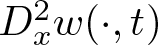 $D^2_x w(\cdot, t)$ is constant. Moreover, called
 $\ell(t)$ such value, we have that
 $t \in (0,T)
\mapsto \ell(t) \in \mathbb{N}$ is nondecreasing.
If moreover  $w$ is spacetime-convex and
 $\widetilde{\mathscr{B}}(\cdot, \cdot, \tilde{p}, \cdot)$ locally convex for each
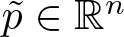 $\tilde{p} \in \mathbb{R}^n$, then the same conclusion as above applies to
 $D^2 w(\cdot, t)$.
Remark 3.12. We observe the following facts.
• The above result will be applied in the following way: let
$u$ be a solution of our Dirichlet problem, and $v=\varphi(u)$ its concave transformation. Then $w:= -v$ is convex and satisfies an equation as (3.8). By [Reference Gallo, Mosconi and Squassina31, Proposition 2.6] and the Dirichlet boundary condition, for each $t$ the matrix $D^2_x w(\cdot,t)$ has full rank in a point (equal to $n$). Thus, by the above constant rank theorem, it is maximum in the whole $\Omega$, and hence here $w$ is strictly convex for each $t$. That is, $v(\cdot, t)$ is strictly concave for each $t$.If
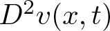
$w$ is also spacetime-convex, then $D^2 v(x,t)$ has constant rank for each $t$, and it can be equal to $n$ or $n+1$; more precisely, by the monotonicity, it is equal to $n$ in $(0,t_0)$ and equal to $n+1$ in $(t_0,+\infty)$ for some $t_0 \in [0,+\infty]$.• In the elliptic case [Reference Korevaar and Lewis50], the condition
$\widetilde{\mathscr{B}}(\cdot, \cdot, \tilde{p}, \cdot)$ convex can be substituted by $\widetilde{\mathscr{B}}(\cdot, \cdot, \tilde{p}, \cdot)$ positive and harmonic convex: as highlighted in [Reference Bian and Guan9], this is essentially related to the fact that the equation $0=\Delta w + \widetilde{\mathscr{B}}(x,w,D_{x}w,t) =: F(D_x^2 w, x, w, D_{x}w, t)$ can be rewritten as $0=\frac{1}{\Delta w} + \frac{1}{\widetilde{\mathscr{B}}(x,w,D_{x}w,t)} =: \bar{F}(D_x^2 w, x, w, D_{x}w, t)$. This is clearly not the case for parabolic equations $w_t =F(D_x^2 w, x, w, D_{x}w, t)$; this is the reason why we obtain the strict concavity in Theorem 1.1 but not in Theorem 1.3. A weaker parabolic counterpart of this generalization can anyway be found in [Reference Bian and Guan9, Theorem 2.3].




4. Concavity and harmonic concavity maximum principles
In this section, we present two maximum principles in the concavity framework, namely Theorem 4.1 and Theorem 4.4.
We start by showing Theorem 4.1, a maximum principle which allows us to relate the interior minimum of the concavity function of a solution  $v$ to the concavity function of the source; in applications,
 $v$ will be the transformation of a solution of a PDE. In this section, we consider a generalization of the result by Korevaar [Reference Korevaar51], by dealing with equations which may include weighted eigenfunctions
 $ u_t - \Delta u = a(x,t) u$. Differently from [Reference Korevaar51], the corresponding
 $\mathscr{B}$ is not required to be nonincreasing w.r.t. the solution
 $v$; actually, we will allow
 $\partial_s \mathscr{B}$ to be also positive, but bounded, in the spirit of [Reference Porru and Serra62] (see also [Reference Greco and Kawohl35]): this permits to study also equations of the type
 $u_t-\Delta u = a(x,t) u \log(u)$ (see [Reference Gallo, Mosconi and Squassina31]). In these results, we look at some concavity of
 $\mathscr{B}$, and we study concavity of
 $u$ in
 $x$ for each
 $t$.
We recall the notation  $p=(\tilde{p}, p^{n+1}) \in \mathbb{R}^{n+1}$.
Theorem 4.1 (Concavity maximum principle)
Let  $T \gt 0$ and
 $v \in C^2_x(\Omega) \cap C^1_t((0,T])$ be such that
 \begin{equation*} - \sum_{i,j=1}^n a_{ij}(D_x v, t) D^2_{ij} v = \mathscr{B}(x,v,D v, t) \quad \hbox{in}\ \Omega \times (0,T] \end{equation*}
where  $\mathscr{B}\colon \Omega\times \mathbb{R}\times \mathbb{R}^{n+1} \times (0,T]\to \mathbb{R} $ locally bounded and
 $(a_{ij}(\tilde{p},t))_{ij}$ is symmetric and positive definite for all
 $(\tilde{p},t)\in \mathbb{R}^{n} \times (0,T]$. Assume that
 $(s, p^{n+1})\in v(\Omega\times [0,T]) \times \mathbb{R} \mapsto \mathscr{B}(x,s,\tilde{p}, p^{n+1}, t)$ is differentiable for all
 $(x,\tilde{p},t)\in \Omega\times \mathbb{R}^{n} \times (0,T]$. Let
 $\mu \in [0,+\infty)$ and suppose
 $e^{-\mu (\star)}\mathcal{C}^*_v$ admits a negative interior minimum at
 $(x_1,x_3,\lambda,t)\in \Omega \times \Omega\times [0,1] \times (0,T]$. Then
 \begin{equation}
\tilde{\xi}:=D_xv(x_1,t)=D_xv(x_2,t)=D_xv(x_3,t).
\end{equation}
Assume moreover
 \begin{equation}
\partial_{p^{n+1}} \mathscr{B} \leq 0
\end{equation}
and that there exists  $\sigma \gt 0 $ such that (it is indeed sufficient to assume
 $\big(\partial_s \mathscr{B}+ \mu \partial_{p^{n+1}} \mathscr{B}\big)\big(x_2, z, \tilde{\xi}, \zeta, t\big) \leq -\sigma$ for any
 $z \in [v_2(t), \lambda v_3(t)+(1-\lambda)v_1(t)]$ and
 $\zeta \in [v_t(x_2,t), \lambda v_t(x_3,t) + (1-\lambda) v_t(x_1,t)]$)
 \begin{equation}
\partial_s \mathscr{B} + \mu \partial_{p^{n+1}} \mathscr{B} \leq -\sigma \lt 0.
\end{equation}
Then
 \begin{equation*} \inf_{\Omega \times \Omega \times [0,1] \times (0,T]} \left( e^{-\mu (\star)}\mathcal{C}^*_v \right) \geq \frac{e^{-\mu t}}{\sigma} \mathcal{C}^*_{\mathscr{B}(\cdot, v(\cdot, \star), \tilde{\xi}, v_t(\cdot, \star), \star)} (x_1, x_3, \lambda, t).\end{equation*}
As a consequence, set  $\rho:=\min \left\{d(x_1,\partial\Omega),d(x_3,\partial \Omega)\right\} \gt 0$, we have
 \begin{equation}
\inf_{\Omega \times \Omega \times [0,1] \times (0,T]} \mathcal{C}^*_v \geq - \frac{e^{\mu T}}{\sigma} \sup_{\Omega_{\rho} \times \Omega_{\rho} \times [0,1] \times (0,T]} \left(\mathcal{C}^*_{\mathscr{B}(\cdot, v(\cdot, \star), \tilde{\xi}, v_t(\cdot, \star), \star)}\right)^- .
\end{equation}
Proof. Let us perform a drift in time and define
 \begin{equation}
w(x,t):= e^{-\mu t} v(x,t)
\end{equation}
which satisfies
 \begin{align*}
- \sum_{i,j=1}^n a_{ij}(e^{\mu t} D_x w, t) D^2_{ij} w
&= e^{-\mu t} \mathscr{B}\big(x, e^{\mu t} w, e^{\mu t} D_x w, e^{\mu t} (\mu w + w_t), t\big) \\
&=: \widehat{\mathscr{B}}(x,w, D w, t) \quad \hbox{in}\ \Omega \times (0,T].
\end{align*}
Notice that
 \begin{equation*}
\begin{aligned}
(\partial_{p^{n+1}}\widehat{\mathscr{B}})(x,s,p,t) = (\partial_{p^{n+1}} \mathscr{B}) \big(x, e^{\mu t} s, e^{\mu t} \tilde{p}, e^{\mu t}(\mu s+p_{n+1}), t\big),
\\
(\partial_s\widehat{\mathscr{B}})(x,s,p,t) = \, (\partial_s \mathscr{B} + \mu \partial_{p^{n+1}} \mathscr{B}) \big(x, e^{\mu t} s, e^{\mu t} \tilde{p}, e^{\mu t}(\mu s+p_{n+1}), t\big),
\end{aligned}
\end{equation*}
thus assumptions (4.2) and (4.3) read
 \begin{equation}
\partial_{p^{n+1}}\widehat{\mathscr{B}} \leq 0
\end{equation}
 \begin{equation}
\partial_s\widehat{\mathscr{B}} \leq -\sigma \lt 0.
\end{equation}
We notice that  $(x_1,x_3,\lambda, t)$ is an interior minimum for
 $\mathcal{C}^*_w$; since it is an interior critical point (with respect to the spatial variable), we obtain
 \begin{equation*}\bar{\xi} := D_x w(x_1,t)=D_x w(x_2,t)=D_x w(x_3,t),\end{equation*}
and thus (4.1) holds, with  $\tilde{\xi} = e^{\mu t} \bar{\xi}$. Exploiting that it is an interior minimum (thus the Hessian matrix with respect to the spatial variable is positive semidefinite) and the positive definiteness of
 $a_{ij}(e^{\mu t} \bar{\xi}, t)$, by [Reference Kennington49, Lemma A.1] we obtain
 \begin{align*}&\sum_{i,j=1}^n a_{ij}(e^{\mu t}\bar{\xi}, t) D^2_{ij} w(x_2, t) - \lambda \sum_{i,j=1}^n a_{ij}(e^{\mu t}\bar{\xi}, t) D^2_{ij} w(x_3, t) - (1-\lambda) \\ &\quad\times \sum_{i,j=1}^n a_{ij}(e^{\mu t} \bar{\xi}, t) D^2_{ij} w(x_1, t) \geq 0\end{align*}
and thus, by the equation,
 \begin{align*}\widehat{\mathscr{B}}\big(x_2, w_2(t), \bar{\xi}, w_t(x_2,t), t\big) & \leq \lambda \widehat{\mathscr{B}}\big(x_3, w_3(t), \bar{\xi}, w_t(x_3,t), t\big)+ (1-\lambda)\\ &\quad\times \widehat{\mathscr{B}}\big(x_1, w_1(t),\bar{\xi}, w_t(x_1,t), t\big) .\end{align*}
Subtracting  $\widehat{\mathscr{B}}\big(x_2, \lambda w_3(t)+(1-\lambda)w_1(t), \bar{\xi}, \lambda w_t(x_3,t) + (1-\lambda) w_t(x_1,t), t\big)$ on both sides and applying Lagrange theorem, we know that there exists
 $z\in [w_2(t),\lambda w_3(t)+(1-\lambda)w_1(t)]$ and
 $\zeta \in [w_t(x_2,t), \lambda w_t(x_3,t) + (1-\lambda) w_t(x_1,t)]$ such that
 \begin{align*}
& \nabla_{s,p^{n+1}}\widehat{\mathscr{B}}(x_2, z, \bar{\xi}, \zeta, t) \cdot \big(\mathcal{C}^*_w(x_1,x_3,\lambda,t), \partial_t \mathcal{C}^*_w(x_1,x_3,\lambda, t)\big) \\ &\quad \leq - \mathcal{C}^*_{\widehat{\mathscr{B}}(\cdot, w(\cdot, \star), \bar{\xi}, w_t(\cdot, \star), \star)} (x_1, x_3, \lambda, t).
\end{align*}
Using that  $(x_1,x_3,\lambda, t)$ is a minimum (with respect to the time variable), we obtain
 \begin{equation*}\partial_t \mathcal{C}^*_w(x_1,x_3, \lambda, t) \leq 0,\end{equation*}
which plugged in the previous inequality together with (4.6) implies
 \begin{equation*}
\partial_s \widehat{\mathscr{B}}(x_2, z, \bar{\xi}, \zeta, t) \mathcal{C}^*_w(x_1,x_3,\lambda,t) \leq - \mathcal{C}^*_{\widehat{\mathscr{B}}(\cdot, w(\cdot, \star), \bar{\xi}, w_t(\cdot, \star), \star)} (x_1, x_3, \lambda, t).
\end{equation*}
By (4.7) and  $\mathcal{C}^*_w(x_1,x_3,\lambda,t) \lt 0$, we achieve
 \begin{equation}
-\sigma \mathcal{C}^*_w(x_1,x_3,\lambda,t) \leq - \mathcal{C}^*_{\widehat{\mathscr{B}}(\cdot, w(\cdot, \star), \bar{\xi}
, w_t(\cdot, \star), \star)} (x_1, x_3, \lambda, t)
\end{equation}
and thus
 \begin{equation*} e^{-\mu t}\mathcal{C}^*_v(x_1,x_3,\lambda,t) \geq \frac{e^{-\mu t}}{\sigma} \mathcal{C}^*_{\mathscr{B}(\cdot, v(\cdot, \star), \tilde{\xi}, v_t(\cdot, \star), \star)} (x_1, x_3, \lambda, t)\end{equation*}
which is the first claim. As a consequence
 \begin{align*}
\inf_{\Omega \times \Omega \times [0,1] \times (0,T]} \left( e^{-\mu (\star)}\mathcal{C}^*_v \right)
&\geq - \frac{e^{-\mu t}}{\sigma} \sup_{\Omega_{\rho} \times \Omega_{\rho} \times [0,1] \times (0,T]} \left(\mathcal{C}^*_{\mathscr{B}(\cdot, v(\cdot, \star), \tilde{\xi}, v_t(\cdot, \star), \star)}\right)^- \\
&\geq - \frac{1}{\sigma} \sup_{\Omega_{\rho} \times \Omega_{\rho} \times [0,1] \times (0,T]} \left(\mathcal{C}^*_{\mathscr{B}(\cdot, v(\cdot, \star), \tilde{\xi}, v_t(\cdot, \star), \star)}\right)^-
\end{align*}
and hence the second claim, observed that (recall that  $ \inf_{\Omega \times \Omega \times [0,1] \times (0,T]} \left( e^{-\mu (\star)}\mathcal{C}^*_v \right) \lt 0$)
 \begin{align*} \inf_{\Omega \times \Omega \times [0,1] \times (0,T]} \mathcal{C}^*_v & = \inf_{\Omega \times \Omega \times [0,1] \times (0,T]} \left( e^{\mu (\star)} e^{-\mu (\star)}\mathcal{C}^*_v\right)\\ & \geq e^{\mu T} \inf_{\Omega \times \Omega \times [0,1] \times (0,T]} \left(e^{-\mu (\star)}\mathcal{C}^*_v\right) . \end{align*}
Remark 4.2. We observe that the quantity  $\rho$ given in Theorem 4.1 and appearing in (4.4) is generally not known: indeed, it is related to the localization of the minimum of the concavity function, which is not an easy task even in simple elliptic equations in simple domains. Since, without any additional information on the equations and on the boundary conditions, the function
 $\mathscr{B}(\cdot, v(\cdot, \star), \tilde{\xi}, v_t(\cdot, \star), \star)$ may explode on the boundary, the presence of such
 $\rho$ allows to deduce anyway a quantitative estimate. In some models, anyway, the dependence on
 $\rho$ could be omitted by exploiting the trivial inequality
 \begin{equation*} \sup_{\Omega_{\rho} \times \Omega_{\rho} \times [0,1] \times (0,T]} \left(\mathcal{C}^*_{\mathscr{B}(\cdot, v(\cdot, \star), \tilde{\xi}, v_t(\cdot, \star), \star)}\right)^- \leq \sup_{\Omega \times \Omega \times [0,1] \times (0,T]} \left(\mathcal{C}^*_{\mathscr{B}(\cdot, v(\cdot, \star), \tilde{\xi}, v_t(\cdot, \star), \star)}\right)^- \end{equation*}
see for instance Corollary 5.6 and Theorem 1.5.
Remark 4.3. If  $\mathscr{B}(x,v,D v, t) \equiv \widetilde{\mathscr{B}}(x,v,D_x v, t) - v_t$, as in the heat equation, we see that
 $\partial_{p^{n+1}} \mathscr{B} = - 1 \leq 0$, while
 \begin{equation*}\partial_s \mathscr{B} + \mu \partial_{p^{n+1}} \mathscr{B} \equiv \partial_s\widetilde{\mathscr{B}} - \mu \leq \Lambda - \mu \leq -\sigma \lt 0\end{equation*}
is satisfied if  $\partial_s \widetilde{\mathscr{B}}$ is bounded from above by some
 $\Lambda \in \mathbb{R}$ and
 $\mu$ is sufficiently large (
 $\mu \gt \Lambda$).
We show now a maximum principle which allows us to relate the interior minimum of the concavity function of a solution  $v$ to the harmonic concavity function of the source. Notice that here we need the source to enjoy some strict monotonicity in
 $v$, see (4.10) (differently from Theorem 4.1, compare with (4.3)). In these results, we look at some harmonic concavity (rather than concavity) of
 $\mathscr{B}$, and we study concavity of
 $u$ in
 $(x,t)$ (rather than concavity in
 $x$ for each
 $t$).
Theorem 4.4 (Harmonic concavity maximum principle)
Let  $v\in C^2_x(\Omega) \cap C^1_t((0,+\infty))$ be such that
 \begin{equation*}
- \sum_{i,j=1}^{n}a_{ij}(Dv)D^2_{ij}v = \mathscr{B}(x,v,Dv, t) \quad \hbox{in}\ \Omega \times (0,+\infty),
\end{equation*}
where  $\mathscr{B}\colon\Omega\times \mathbb{R}\times \mathbb{R}^{n+1} \times (0,+\infty)\to \mathbb{R} $ and
 $(a_{ij}(p))_{ij}$ is symmetric and positive definite for all
 $p\in \mathbb{R}^{n+1}$. Assume that
 $s \in v(\Omega\times [0,+\infty)) \mapsto \mathscr{B}(x,s,p,t)$ is differentiable for all
 $(x,p,t)\in \Omega\times \mathbb{R}^{n+1} \times (0,+\infty)$. Suppose
 $\mathcal{C}_v$ admits a negative interior minimum at
 $(x_1,x_3,t_1,t_3,\lambda)\in \Omega \times \Omega \times (0,+\infty)\times (0,+\infty)\times [0,1]$. Then
 \begin{equation}
\xi:=Dv(x_1,t_1)=Dv(x_2,t_2)=Dv(x_3,t_3).
\end{equation}
Assume moreover that there exists  $\sigma \gt 0$ such that
 \begin{equation}
\sup_{z\in [v(x_2,t_2),\lambda v(x_3,t_3)+(1-\lambda)v(x_1,t_1)]} \partial_s\mathscr{B}(x_2,z,\xi, t_2)\leq-\sigma.
\end{equation}
Then
 \begin{equation}
\inf_{\Omega\times \Omega \times (0,+\infty)\times (0,+\infty)\times[0,1]}\mathcal{C}_v\geq \dfrac{1}{\sigma} \mathcal{HC}_{\mathscr{B}(\cdot, v(\cdot,\star), \xi, \star)}(x_1,x_3,t_1,t_3,\lambda).
\end{equation}
Proof. Notice first that  $(x_1,t_1)\ne (x_3,t_3)$ and
 $\lambda\in (0,1)$, otherwise
 $\mathcal{C}_v(x_1,x_3,t_1,t_3,\lambda)=0$, which is a contradiction. Being
 $(x_1,x_3,t_1,t_3,\lambda)$ in the interior of the domain we obtain
 \begin{equation*} D\mathcal{C}_v(x_1,x_3,t_1,t_3,\lambda)=0 \end{equation*}
and in particular  $D_{y_1}\mathcal{C}_v = D_{y_3}\mathcal{C}_v = D_{\tau_1}\mathcal{C}_v = D_{\tau_3}\mathcal{C}_v = 0$ imply (4.9). Set now
 $A:=(a_{ij}(\xi))_{ij}$ and define the
 $2n\times 2n$ matrices
 \begin{equation*} C:=
\begin{bmatrix}
D^2_{y_1, y_1}\mathcal{C}_v(x_1,x_3, t_1,t_3,\lambda) & D^2_{y_1, y_3}\mathcal{C}_v(x_1,x_3, t_1,t_3,\lambda)\\
D^2_{y_1, y_3}\mathcal{C}_v(x_1,x_3, t_1,t_3,\lambda) & D^2_{y_3, y_3}\mathcal{C}_v(x_1,x_3, t_1,t_3,\lambda)
\end{bmatrix}, \end{equation*}
which is positive semidefinite since  $(x_1,x_3, t_1,t_3,\lambda)$ is a minimum for
 $\mathcal{C}_v$ and
 \begin{equation*} B:= \begin{bmatrix}
s^2a_{ij}(\xi) & sra_{ij}(\xi) \\
sra_{ij}(\xi) & r^2a_{ij}(\xi)
\end{bmatrix}, \end{equation*}
which is positive semidefinite by hypothesis. So by [Reference Kennington49, Lemma A.1] we have  ${\rm Tr}(BC)\geq 0$, that is
 \begin{equation}
\alpha s^2 +2\beta sr +\gamma r^2\geq 0 \quad \hbox{for all}\ s,r\in \mathbb{R}
\end{equation}
where
 \begin{equation*} \alpha := {\rm Tr} (AD^2_{y_1,y_1}\mathcal{C}_v), \quad \beta:= {\rm Tr} (AD^2_{y_1,y_3}\mathcal{C}_v),\quad \gamma:= {\rm Tr} (AD^2_{y_3,y_3}\mathcal{C}_v),\end{equation*}
which rewrite as
 \begin{equation*}
\alpha =(1-\lambda)^2Q_2-(1-\lambda)Q_1, \qquad \beta= \lambda(1-\lambda)Q_2, \qquad \gamma= \lambda^2Q_2-\lambda Q_3,
\end{equation*}
where we have set for  $k\in\left\{1,2,3\right\}$
 \begin{equation*} Q_k:=\sum_{i,j=1}^na_{ij}D^2_{ij}v(x_k,t_k).\end{equation*}
By (4.12) we obtain  $\alpha\geq0, \gamma\geq0$ and
 $\beta^2-\alpha \gamma\leq0$, i.e.
 \begin{equation}
Q_2\geq \dfrac{Q_1}{1-\lambda},
\end{equation}
 \begin{equation}
Q_2\geq \dfrac{Q_3}{\lambda},
\end{equation}
 \begin{equation}
Q_1Q_3\geq Q_2((1-\lambda)Q_3+\lambda Q_1),
\end{equation}
where we justify the last by
 \begin{equation*}
\begin{split}
0&\geq \lambda^2(1-\lambda)^2Q_2^2-((1-\lambda)^2Q_2-(1-\lambda)Q_1)(\lambda^2 Q_2-\lambda Q_3)\\
& =\lambda(1-\lambda)((1-\lambda)Q_2Q_3+\lambda Q_2Q_1-Q_1Q_3).
\end{split}
\end{equation*}
Claim:  $(1-\lambda)Q_3+\lambda Q_1 \lt 0$ or
 $Q_1=Q_3=0$.
If  $(1-\lambda)Q_3+\lambda Q_1\geq0$, then by (4.13) and (4.15)
 \begin{align*}
Q_2 \big( (1-\lambda)Q_3+\lambda Q_1 \big)&\geq \frac{Q_1}{1-\lambda}\big( (1-\lambda)Q_3+\lambda Q_1\big),\\
Q_2\big( (1-\lambda)Q_3+\lambda Q_1 \big)&\geq Q_1Q_3+\frac{\lambda}{1-\lambda}Q_1^2,\\
Q_2\big( (1-\lambda)Q_3+\lambda Q_1 \big)&\geq Q_2\big( (1-\lambda)Q_3+\lambda Q_1 \big)+\frac{\lambda}{1-\lambda}Q_1^2,
\end{align*}
which imply  $Q_1=0$. Similarly (exploiting (4.14) and (4.15)), we have
 $Q_3=0$. Then if
 $(1-\lambda)Q_3+\lambda Q_1 \lt 0$ and from (4.15), it holds
 \begin{equation*} Q_2\geq \dfrac{Q_1Q_3}{(1-\lambda)Q_3+\lambda Q_1}. \end{equation*}
Being  $Q_k = -\mathscr{B}\big(x_k,v_k, \xi, t_k\big)$, we get
 \begin{align*}
-\mathscr{B}\big(x_2,v_2,\xi, t_2\big)\geq - \dfrac{\mathscr{B}\big(x_1,v_1,\xi, t_1\big)\mathscr{B}(x_3,v_3,\xi, t_3\big)}{(1-\lambda)\mathscr{B}\big(x_3,v_3,\xi, t_3\big)+\lambda \mathscr{B}\big(x_1,v_1,\xi, t_1\big)}.
\end{align*}
Adding on both sides  $\mathscr{B}\big(x_2,\lambda v_3+(1-\lambda)v_1,\xi, t_2\big)$ and applying Lagrange theorem, we obtain
 \begin{equation*}-\partial_s\mathscr{B}(x_2,z,\xi, t_2)\mathcal{C}_v(x_1,x_3,t_1,t_3,\lambda)\geq \mathcal{HC}_{\mathscr{B}(\cdot, v(\cdot,\star),\xi, \star)}(x_1,x_3,t_1,t_3,\lambda)\end{equation*}
for some  $z\in [v_2,\lambda v_3+(1-\lambda)v_1]$. Otherwise, if
 $Q_1=Q_3=0$, then
 $Q_2\geq 0$ and by the same arguments as before it holds
 \begin{equation*} -\partial_s\mathscr{B}(x_2,z,\xi, t_2)\mathcal{C}_v(x_1,x_3,t_1,t_3,\lambda)\geq \mathcal{HC}_{\mathscr{B}(\cdot, v(\cdot,\star),\xi,\star)}(x_1,x_3,t_1,t_3,\lambda).\end{equation*}
Since  $\mathcal{C}_v(x_1,x_3,t_1,t_3,\lambda) \lt 0$ and
 $\partial_s \mathscr{B}(x_2,z,\xi, t_2)\leq-\sigma$, in any case it follows that
 \begin{align*} \sigma \mathcal{C}_v(x_1,x_3,t_1,t_3,\lambda)& \geq -\partial_s\mathscr{B}(x_2,z,\xi,t_2)\mathcal{C}_v(x_1,x_3,t_1,t_3,\lambda)\\ &\geq \mathcal{HC}_{\mathscr{B}(\cdot, v(\cdot,\star),\xi,\star)}(x_1,x_3,t_1,t_3,\lambda), \end{align*}
and thus the claim.
We see that, in Theorem 4.4, the nonlinear term  $\mathscr{B}$ actually includes
 $v_t$ in any form. In the special case of heat-type equations, we can remove the dependence on the right side of (4.11) from
 $ v_t$ by assuming
 $v$ monotone.
Corollary 4.5. In the setting of Theorem 4.4, assume that  $\mathscr{B}$ has the form
 \begin{equation*}\mathscr{B}(x, v, Dv, t) \equiv \widetilde{\mathscr{B}}(x,v, D_x v, t) - k(t) v_t\end{equation*}
with  $\mathcal{HC}_{k} \leq 0$ (for instance,
 $k$ is constant). Assume moreover that
 $\xi^{n+1} \geq 0$ (recall
 $\xi^{n+1}= v_t(x_1,t_1)= v_t(x_2,t_2)= v_t(x_3,t_3)$) and
 $k \gt 0$. Then
 \begin{equation*} \inf_{\Omega\times \Omega \times (0,+\infty)\times (0,+\infty)\times[0,1]}\mathcal{C}_v\geq \dfrac{1}{\sigma} \mathcal{HC}_{\widetilde{\mathscr{B}}(\cdot, v(\cdot,\star), \tilde{\xi},\star)}(x_1,x_3,t_1,t_3,\lambda). \end{equation*}
Proof. It is sufficient to apply Theorem 4.4 and Proposition B.4 (notice that if  $\xi^{n+1}=0$ the claim is obvious).
Remark 4.6. We notice in Corollary 4.5, the essential role of  $ v_t$ being constant on
 $(x_1,t_1)$,
 $(x_2,t_2)$,
 $(x_3,t_3)$. This is a consequence of the fact that we study the space-time concavity in
 $(0,+\infty)$ (and not only space concavity in
 $(0,T]$).
5. Maximum principles with boundary conditions
In Section 4, we dealt with the value of the concavity function in the interior of the domain. In this section, we focus on the behaviour on the boundary: to this aim, we consider a Dirichlet boundary condition and a Cauchy initial datum. For the sake of simplicity, we focus now on equations of heat type, that is, with main operator 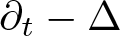 $\partial_t - \Delta$.
5.1. Concavity
In this subsection, we apply Theorem 4.1 to  $v$, transformation of a solution
 $u$ of a Cauchy–Dirichlet problem.
Theorem 5.1 (Estimate on log-concavity)
Let  $\Omega \subset \mathbb{R}^n$,
 $n\geq 2$, be a bounded, smooth, strongly convex domain. Let
 $T \gt 0$,
 $b\colon \Omega \times (0,+\infty) \times (0,T]\to \mathbb{R}$,
 $b(x,\cdot, t)$ differentiable for all
 $(x,t)\in \Omega\times (0,T]$,
 $u_0\in C^1(\overline{\Omega})$ with
 $u_0=0$ on
 $\partial\Omega$ and
 $u \in C^2_x(\overline{\Omega}) \cap
C^1(\overline{\Omega}\times[0,T])$, be such that
 \begin{equation*}u_t - \Delta u = b(x,u, t) \quad \hbox{in}\ \Omega \times (0,T]\end{equation*}
with
 \begin{equation}
\begin{cases}
u \gt 0 & \text{in } \Omega\times (0,T],\\
u=0 & \text{on }\partial \Omega \times[0,T],\\
D_x u \cdot \nu \gt 0 & \text{on }\partial \Omega\times [0,T], \\
u =u_0 & \text{on } \overline{\Omega} \times \{0\}.
\end{cases}
\end{equation}
Assume there exists  $\Lambda \geq 0$ such that
 \begin{equation*}\partial_s \big(e^{-s} b(x,e^{s}, t)\big) \leq \Lambda \quad \hbox{for each}\ (x,s, t) \in \Omega \times \mathbb{R} \times (0,T].\end{equation*}
Assume moreover that  $u_0 \gt 0$ is
 $\log$-concave in
 $\Omega$. Then there exists
 $\rho \gt 0$ such that
 \begin{equation}
\inf_{\Omega \times \Omega \times [0,1] \times [0,T]} \mathcal{C}^*_{\log(u)} \geq -T e^{1+\Lambda T} \sup_{\Omega_{\rho} \times \Omega_{\rho} \times [0,1] \times (0,T]} \left(\mathcal{C}^*_{\frac{b(\cdot, u(\cdot, \star), \star)}{u(\cdot,\star)} }\right)^-.
\end{equation}
Proof. We see that  $v:=\log(u)$ solves (exploiting the notation in Remark 4.3)
 \begin{equation*}v_t - \Delta v = e^{-v} b(x, e^v, t) + |D_x v|^2 =: \widetilde{\mathscr{B}}(x,v,D_x v, t) \quad \hbox{in}\ \Omega \times (0,T]\end{equation*}
with 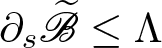 $\partial_s \widetilde{\mathscr{B}} \leq \Lambda$. If
 $ \mathcal{C}^*_v \geq 0$ the claim holds. Otherwise, assume that
 $ \mathcal{C}^*_v$ is somewhere negative. Let
 $\mu \gt \Lambda$. By the assumption on the initial condition, the function
 $e^{-\mu t}\mathcal{C}_v^*(x_1,x_3,\lambda, t)$ cannot get negative for
 $(x_1,x_3,\lambda,t) $ approaching
 $\overline{\Omega} \times \overline{\Omega}\times[0,1]\times\{0\}$. Let now by contradiction
 $(x_1^n,x_3^n,\lambda^n, t^n)$ be a minimizing sequence for
 $e^{-\mu t}\mathcal{C}_v^*$ approaching
 $\partial (\Omega \times \Omega) \times[0,1]\times(0,T]$; up to a subsequence
 $t_n \to t \in (0,+\infty)$. By
 $D_x u \cdot \nu \gt 0 $ we easily obtain
 $u(x_i^n, t^n)/u(x_i^n, t) \to 1$, i.e.
 $v(x_i^n, t^n) - v(x_i^n, t) \to 0$; this ensures that
 $(x_1^n,x_3^n,\lambda^n, t)$ is a minimizing sequence as well. Consider
 $u(\cdot, t)$: by the assumption on the boundary coupled with [Reference Korevaar51, Lemma 2.4] (see also [Reference Gallo and Squassina32, Proposition 4.6]), the function
 $e^{-\mu t}\mathcal{C}_v^*(x_1^n,x_3^n,\lambda^n, t)$ is positively far from zero, which is absurd.
Then  $e^{-\mu t}\mathcal{C}_v^*(x_1,x_3,\lambda, t)$ must admit an interior negative minimum. Thus, by Theorem 4.1, we obtain
 \begin{equation*}
\inf_{\Omega \times \Omega \times [0,1] \times (0,T]} \mathcal{C}^*_v \geq - \frac{e^{\mu T}}{\mu-\Lambda}
\sup_{\Omega_{\rho} \times \Omega_{\rho} \times [0,1] \times (0,T]} \left(\mathcal{C}^*_{e^{-v(\cdot, \star)} b(\cdot, e^{v(\cdot, \star)}, \star)}\right)^- .
\end{equation*}
Since the choice of  $\mu \gt \Lambda$ is arbitrary, we maximize the right-hand side (which is the case for
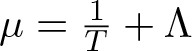 $\mu=\frac{1}{T}+\Lambda$) and conclude.
Let us remark that, in Theorem 5.1, if 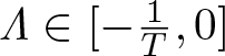 $\mathit\Lambda \in [-\frac{1}{T},0]$, the claim holds as well; if instead
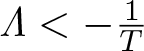 $\mathit\Lambda \lt -\frac{1}{T}$, then the coefficient on the right-hand side of (5.2) does not depend on
 $T$ and equals
 $-\frac{1}{|\mathit\Lambda|}$.
Remark 5.2. If in Theorem 5.1, we do not assume  $u_0$ to be
 $\log$-concave, then we take into account also
 $ \mathcal{C}_{\log(u_0)}$, obtaining
 \begin{align*}&\inf_{\Omega \times \Omega \times [0,1] \times [0,T]} \mathcal{C}^*_{\log(u)}\\ &\qquad \geq -\max\left \{T e^{1+\Lambda T} \sup_{\Omega_{\rho} \times \Omega_{\rho} \times [0,1] \times (0,T]} \left(\mathcal{C}^*_{\frac{b(\cdot, u(\cdot, \star), \star)}{u(\cdot,\star)} }\right)^-, \sup_{\Omega \times \Omega \times [0,1]} \mathcal{C}_{\log(u_0)}^- \right\}.\end{align*}
Indeed, as in the previous proof, the negative infimum is far from  $\partial(\Omega \times \Omega) \times [0,1]\times (0,T]$; if there is an interior minimum, then the previous reasoning applies and (5.2) holds. If instead the infimum is realized for
 $(x_1,x_3,\lambda,t) \to \overline{\Omega} \times \overline{\Omega}\times[0,1]\times\{0\}$, then it means
 \begin{equation*}\inf_{\Omega \times \Omega \times [0,1] \times [0,T]} \mathcal{C}^*_{\log(u)} \geq
\inf_{\Omega \times \Omega \times [0,1]} \left(-\mathcal{C}_{\log(u_0)}^- \right).\end{equation*}
Joining the two possibilities, we obtain the claim.
Corollary 5.3 (Exact log-concavity)
In the assumptions of Theorem 5.1 assume moreover that
•
$(s,x) \mapsto s^{-1} b(x,s,t)$ is concave for each $t \gt 0$.


Then  $u(\cdot, t)$ is
 $\log$-concave for each
 $t\in (0,T)
$. Moreover if
 $b\in C^{2,1}(\Omega\times(0,+\infty)\times [0,T))$ and
 $u \in C^{2,1}(\Omega \times [0,T))$, then
 $u(\cdot, t)$ is strictly
 $\log$-concave for each
 $t\in (0,T)
$.
Proof. By Theorem 5.1, we obtain that  $v=\log(u)$ is concave. Arguing as in Remark 3.12 and applying Proposition 3.11 to
 $w=-v$, we obtain the strict concavity.
5.1.1. Applications
Proof of Theorem 1.1 and Theorem 1.2
They are a consequence of Corollary 5.3 and Proposition 3.9 (iv).
Remark 5.4. We deduced strict concavity in Theorem 1.1 thanks to the constant rank theorem. In the eigenfunction case  $b(x,s,t)=a(x,t)s$, by assuming
 $a(\cdot, t)$ strictly concave for each
 $t \gt 0$, we can reach the same claim in a more straightforward way.
Indeed, assume by contradiction that there exists  $t \gt 0$ and
 $x_1 \neq x_3$,
 $\lambda \in (0,1)$ such that
 $\mathcal{C}^*_{\log(u)}(x_1, x_3, \lambda, t) = 0$. Recalled that we already proved
 $\mathcal{C}^*_{\log(u)}\geq 0$, in the notations of the proof of Theorem 4.1—fixed a whatever
 $\mu \gt 0$—we have
 $w=e^{-\mu t} v = e^{-\mu t} \log(u)$, thus
 $\mathcal{C}^*_{w} \geq 0 = \mathcal{C}^*_w(x_1,x_3,\lambda, t)$, and hence
 $(x_1,x_3,\lambda, t)$ is a point of minimum for
 $\mathcal{C}^*_w$. Thus by (4.8) we obtain
 \begin{equation*} 0 \leq - \mathcal{C}^*_{\widetilde{\mathscr{B}}(\cdot, w(\cdot, \star), \xi, \star)} (x_1, x_3, \lambda, t)
= - e^{-\mu t} \mathcal{C}^*_{a(x,t) } (x_1,x_3,\lambda, t) \lt 0, \end{equation*}
thanks to the strict concavity of  $a$ and the assumption
 $x_1 \neq x_3$,
 $\lambda \in (0,1)$. This contradiction concludes the proof.
Remark 5.5. We mention that Theorem 4.1 has interesting applications also in gradient-type equations. For instance, consider the evolutionary equation driven by the Ornstein–Uhlenbeck operator
 \begin{equation*}\partial_t u - \Delta u = -x \cdot \nabla u \quad \hbox{in}\ \Omega \times (0,+\infty)\end{equation*}
with  $u=0$ on
 $\partial \Omega \times (0,+\infty)$ and
 $u=u_0$ on
 $\Omega \times \{t=0\}$. Recently (after the submission of the present paper), the authors in [Reference Colesanti and Salani24] showed that every solution is log-concave in
 $x$ for each
 $t$, as long as
 $u_0$ is chosen
 $\log$-concave and
 $\Omega$ convex. We see that actually we can recover this result if we additionally require
 $\Omega$ strongly convex and
 $u_0 \in C^1(\overline{\Omega})$ with
 $D_x u_0 \cdot \nu \gt 0 $ on
 $\partial \Omega$ (see (5.1) and Lemma A.4). Indeed, reasoning on
 $[0,T]$ for arbitrary
 $T$ fixed, following Remark 4.3,
we have
 $\widetilde{\mathscr{B}}(x,s,\tilde{p}, t) = - x \cdot \tilde{p}+ |\tilde{p}|^2$, and hence
 $\partial_s \widetilde{\mathscr{B}}=0$. Moreover,
 $(x,s) \mapsto \widetilde{\mathscr{B}}(x,s,\tilde{p}, t)$ is concave. Arguing as in Theorem 5.1, we have that the minimum is in the interior; thus, Theorem 4.1 implies the claim. Differently from [Reference Colesanti and Salani24], we do not rely on an integral representation of the solution; thus, the result can be easily extended to more general drift Laplacians, e.g. of the form
 $\Delta u -V(x,t) \cdot \nabla u$.
We focus now on perturbed concavity as a consequence of Theorem 5.1. Exploiting it together with Propositions B.1 and B.2, we obtain the following statement. Notice that  $\{\partial_r(e^{-r} f(e^r)) \mid r \in \mathbb{R}\} \equiv \{s \partial_s( s^{-1} f(s)) \mid s \gt 0\} $.
Corollary 5.6. Let  $\Omega \subset \mathbb{R}^n$,
 $n\geq 2$, be a bounded, smooth, strongly convex domain. Let
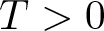 $T \gt 0$,
 $a\colon\Omega\times(0,T]\to \mathbb{R}$ locally bounded,
 $f\colon(0,+\infty)\to\mathbb{R}$ differentiable,
 $u_0\in C^1(\overline{\Omega})$ with
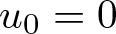 $u_0=0$ on
 $\partial\Omega$ and
 $u \in C^2_x(\overline{\Omega}) \cap C^1
(\overline{\Omega}\times [0,T])$ be such that
 \begin{equation*}u_t - \Delta u = a(x,t) f(u)\quad \hbox{in}\ \Omega \times (0,T]\end{equation*}
with (5.1). Set 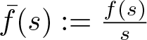 $\bar{f}(s):= \frac{f(s)}{s} $ for
 $s \gt 0$ and assume
 \begin{equation*}\Lambda:=\sup_{(x,s,t) \in \Omega \times(0,+\infty)\times (0,T]}
\big(a(x,t) s \bar{f}'(s) \big) \lt + \infty.\end{equation*}
Assume moreover that  $u_0 \gt 0$ is
 $\log$-concave in
 $\Omega$. Then there exists
 $\rho \gt 0$ such that the following facts hold.
i) If
$\bar{f}$ is constant, then
\begin{equation*}\inf_{\Omega \times \Omega \times [0,1] \times [0,T]} \mathcal{C}^*_{\log(u)} \geq -T e^{1+\Lambda T} \sup_{\Omega_{\rho} \times \Omega_{\rho} \times [0,1] \times (0,T]} \left(\mathcal{C}^*_{a(\cdot, \star)}\right)^-.\end{equation*}ii) If
$\bar{f}$ is $\theta'$-concave, with $\theta' \gt 1$, and $0 \lt m\leq a \leq M$ with $m^{\theta} \geq \frac{1}{2} M^{\theta}$, $\frac{1}{\theta} + \frac{1}{\theta'}=1$, then
\begin{align*}\inf_{\Omega \times \Omega \times [0,1] \times [0,T]} \mathcal{C}^*_{\log(u)}
& \geq -T e^{1+\Lambda T}
\|\bar{f}(u)\|_{L^{\infty}(\Omega_{\rho}\times (0,T])}\\
&\quad\times \sup_{\Omega_{\rho} \times \Omega_{\rho} \times [0,1] \times (0,T]}
\left( \left(\mathcal{C}^*_{a^{\theta}(\cdot, \star)}\right)^-\right)^{\frac{1}{\theta}}.
\end{align*}iii) If
$\bar{f}$ is concave and $a$ is bounded and nonnegative, then
\begin{equation*}\inf_{\Omega \times \Omega \times [0,1] \times [0,T]} \mathcal{C}^*_{\log(u)} \geq
-T e^{1+\Lambda T}
\|\bar{f}(u)\|_{L^{\infty}(\Omega_{\rho}\times (0,T])}
{\rm osc}(a).
\end{equation*}


We note that Corollary 5.6 applies to the following sources  $f(s)=s$ (case i),
 $f(s)=s\log^q(1+s)$,
 $f(s)=\frac{s^{q+1}}{1+s^q}$ with
 $q\in(0,1)$ (case ii),
 $f(s)=\frac{s^2}{1+s}$,
 $f(s)=s\log(1+s)$,
 $f(s)=s\log(s)$ (case iii).
Proof of Theorem 1.5
It is a particular case of Corollary 5.6.
Remark 5.7. Consider  $b(x,s,t)=s \log(s)$. In [Reference Gallo, Mosconi and Squassina31], the authors show the existence of a
 $\log$-concave solution for the stationary problem; here, in Theorem 1.1, we show the
 $\log$-concavity of the evolutionary solution in each
 $[0,T]$, whenever such solution exists. We discuss the possible (pointwise) convergence of
 $u(x,t)$ to a stationary solution as
 $t\to +\infty$ and, thus, the possibility of achieving the result in [Reference Gallo, Mosconi and Squassina31] through a parabolic approach. We start by noticing that the assumptions in Remark 3.3 are not fulfilled. Let
 $u_0$ be a
 $\log$-concave function. If
 $I(u_0):=|\nabla u_0|_2^2 - \int_{\Omega} u_0^2 \log(u_0) \lt 0$, then by [Reference Han37, Theorem 1.1] we obtain that
 $u(x,t) \to +\infty$ as
 $t \to +\infty$. If
 $I(u_0) \gt 0$, and
 $J(u_0):=I(u_0)+\frac{1}{4} \|u_0\|_2^2\leq \frac {1}{4} (2\pi)^{n/2} e^n=:M$, then by [Reference Chen, Luo and Liu20, Theorems 1.1 and 1.2] we have
 $u(x,t) \to 0$ as
 $t \to +\infty$. If
 $I(u_0)=0$, then by the logarithmic Sobolev inequality and arguing as in [Reference Wang and Wang66, Lemma 2.3], we obtain
 $J(u_0) \geq M$; if
 $J(u_0)=M$, then [Reference Chen, Luo and Liu20, Theorem 1.2] implies
 $u \in L^{\infty}((0,+\infty), H^1_0)$, even if it is not known whether the solution decays to zero or not. The cases
 $I(u_0) \gt 0$ and
 $J(u_0) \gt M$, or
 $I(u_0)=0$ and
 $J(u_0) \gt M$ are—up to the authors’ knowledge—still open problems. We further observe that, similarly to Corollary A.3, if
 $u_0$ is also a subsolution of the stationary problem (in particular,
 $I(u_0) \leq 0$), then we have that
 $u(x, \cdot)$ is nondecreasing, thus a limit must exist. By the above considerations, we have no examples at hand in which the convergence to the stationary solution can be pursued.
Example 5.8. As particular cases of concave  $a$ we may consider
 $a(x,t)=t^{\gamma} d_\Omega(x)^\omega $,
 $\gamma, \omega \in [0,1]$, with
 $\gamma+\omega=1$ (see Proposition 3.9). In such a case, the solutions of
 \begin{equation*} u_t - \Delta u = t^{\gamma} d(x,\partial \Omega)^{\omega} u\end{equation*}
are  $\log$-concave.
As an additional consequence of Theorem 5.1, we may also consider population models [Reference Cantrell and Cosner15].
Corollary 5.9. Let 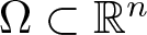 $\Omega \subset \mathbb{R}^n$,
 $n\geq 2$, be a bounded, smooth, strongly convex domain. Let
 $T \gt 0$,
 $a\colon\Omega\times(0,T]\to \mathbb{R}$ bounded,
 $u_0\in C^1(\overline{\Omega})$ with
 $u_0=0$ on
 $\partial\Omega$ and
 $u \in C^2_x(\overline{\Omega}) \cap C^1_t((0,T]) \cap C(\overline{\Omega}\times[0,T])$ be such that
 \begin{equation*}u_t - \Delta u = a(x, t) u - u^2 \quad \hbox{in}\ \Omega \times (0,T]\end{equation*}
with (5.1). Assume moreover that  $u_0 \gt 0$ is
 $\log$-concave in
 $\Omega$. Then there exists
 $\rho \gt 0$ such that
 \begin{equation*}\inf_{\Omega \times \Omega \times [0,1] \times [0,T]} \mathcal{C}^*_{\log(u)} \geq - e T \sup_{\Omega_{\rho} \times \Omega_{\rho} \times [0,1] \times (0,T]} \left(\mathcal{C}^*_{a(\cdot, \star) }\right)^-.\end{equation*}
Remark 5.10. We see that some results in Corollary 5.9 can be extended to piecewise constant weights  $a=a(x)$ arising in bang-bang optimization theory (see [Reference Cantrell and Cosner15, Theorem 3.9]), i.e. equal to
 $a_1 \gt 0$ on some region of
 $\Omega$ and to
 $-a_2 \lt 0$ on some other region. We give just a sketch of the proof. Let indeed
 $a$ be as above, and let
 $a_{\varepsilon} \in L^{\infty}(\mathbb{R}^n)$ be a suitable equibounded regular approximating sequence for
 $a$. Let
 $u_{\varepsilon}$ be positive solutions of
 $\partial_t u_{\varepsilon} -\Delta u_{\varepsilon} = a_{\varepsilon}(x) u_{\varepsilon} - u_{\varepsilon}^2$,
 $u_{\varepsilon} =0$ on
 $\partial \Omega$,
 $u_{\varepsilon}(0)=u_0$. Exploiting that
 $a_{\varepsilon}(x) t -t^2\leq 0$ for
 $t \geq \sup_{\varepsilon} \|a_{\varepsilon}\|_{\infty}$ and the maximum principle we obtain that
 $\|u_{\varepsilon}\|_{\infty}$ is equibounded; then standard regularity theory implies that
 $u_{\varepsilon}$ is also equibounded in some
 $C^{0,\sigma}$, and hence it converges uniformly up to a subsequence by Ascoli–Arzelà theorem. We can thus pass to the limit the weak formulation (see e.g. [Reference Cazenave, Dickstein and Escobedo16]) of the equations and obtain that
 $u_{\varepsilon} \to u$ solution of the equation with weight
 $a(x)$. Since
 $u_{\varepsilon}$ are regular, then they satisfy the assumptions of Corollary 5.9 and thus, in particular,
 $\inf \mathcal{C}^*_{\log(u_{\varepsilon})} \geq - e T \sup\left(\mathcal{C}^*_{a_{\varepsilon}(\cdot, \star) }\right)^- \geq - eT {\rm osc}(a_{\varepsilon})$. Passing to the limit, we obtain
 \begin{equation*}\inf \mathcal{C}^*_{\log(u)} \geq - eT (a_1+a_2).\end{equation*}
We leave the details to the interested reader.
5.2. Harmonic concavity
In this subsection, we consider applications of Cauchy–Dirichlet type to Theorem 4.4. The main assumptions are the following ones.
- Domain:
(5.3)\begin{align}
\Omega \subset \mathbb{R}^n, n\geq 2,\ & \hbox{bounded convex domain which satisfies the interior}\nonumber\\ & \quad \hbox{sphere property.}
\end{align}- Regularity:
(5.4)\begin{equation}
u\in C^2_x(\Omega)\cap C^1_x(\overline{\Omega})\cap C^1_t((0,+\infty))\cap C(\overline{\Omega}\times[0,+\infty)).
\end{equation}- Equation:
(5.5)\begin{equation}
u_t-\Delta u=b(x,u, t) \quad\hbox{in }\Omega\times (0,+\infty).
\end{equation}- Boundary conditions:
(5.6)\begin{equation}
\begin{cases}
u \gt 0 & \text{in } \Omega\times (0,+\infty),\\
u=0 & \text{on }\partial \Omega\times [0,+\infty), \\
u =0 & \text{on } \overline{\Omega} \times \{0\}.
\end{cases}
\end{equation}


Our aim is to deduce a quantitative estimate on the concavity function of a power of  $u$ (see Theorem 5.16). Let us consider a function
 $u\colon\overline{\Omega} \times[0,+\infty)\to \mathbb{R}$ which satisfies (5.6) and the equation (5.5). For
 $\alpha, \beta \gt 0$ set
 \begin{equation}
v(x,t):=u^\alpha(x,t^{\beta}) .
\end{equation}
By some straightforward computations, and recalled that  $v \gt 0$, we have that the equation solved by
 $v$ is
 \begin{equation}
-\Delta v =\mathscr{B} (x,v, Dv, t) \quad\text{in }\Omega\times (0,+\infty),
\end{equation}
where
 \begin{equation}
\begin{aligned}
\mathscr{B}(x,s,p,t) &:= \widetilde{\mathscr{B}}(x,s,\tilde{p},t) -\frac{1}{\beta} t^{1-\beta }p^{n+1} \\
&:= \frac{1-\alpha}{\alpha}\frac{|\tilde{p}|^2}{s}+\alpha s^{\frac{\alpha-1}{\alpha}}b\left(x,s^{1/\alpha}, t^{\beta}\right) -\frac{1}{\beta} t^{1-\beta} p^{n+1}.
\end{aligned}
\end{equation}
To apply Corollary 4.5 to  $v$, we need to ensure that a negative minimum of the concavity function is attained in the interior of
 $\Omega \times (0,+\infty)$ or at infinity. In the following propositions, thus, we rule out the possibility of having a minimum on
 $\partial \Omega$ or
 $t=0$.
We start with some boundary estimates. We also refer to Lemma 6.3 for a version including  $f(x_0,t)=0$ for
 $x_0 \in \partial \Omega$. We also mention [Reference Martel and Souplet59, Theorem 5].
Lemma 5.11 (Boundary estimates)
Let  $\Omega$ satisfy (5.3), and
 $u$ be a function such that (5.4), (5.5) and (5.6) hold. Suppose
 $b\colon\Omega\times(0,+\infty) \times (0,+\infty)\to \mathbb{R}$ satisfies (H1), and consider
 $M, T, q,\gamma, k$ therein; we can assume
 $T$ small enough in such a way
 $\|u\|_{L^{\infty}(\Omega\times[0,T])} \lt M$. The following facts hold.
(i) [Dealing with
$ \Omega \times \{0\}$]: let $\varphi_1$ be the first Dirichlet eigenfunction on $\Omega$ with eigenvalue $\lambda_1$, normalized by $\|\varphi_1\|_{\infty}=1$. Then,
for some explicit\begin{equation*}u(x,t) \geq C e^{-\lambda_1 t} t^{\frac{1+\gamma}{1-q}}\varphi_1(x) \quad \hbox{in}\ \Omega \times (0,T)\end{equation*}$C=C(\|u\|_{L^{\infty}(\Omega \times [0,T])}, q, \gamma, T,k) \gt 0$.(ii) [Dealing with
$\partial \Omega \times \{0\}$]: for any $x_0 \in \partial \Omega$ and $\beta \in (0,2]$, there exists $\delta=\delta(x_0,T, \beta,q,\gamma,k,\Omega) \gt 0$ such that
where\begin{equation*}u(x_0+t\nu,t^{\beta})\geq \delta t^{\frac{2\beta(1+\gamma)+(2-\beta)(1-q) }{2(1-q)}} \quad \hbox{for}\ t\in (0,T)\ \hbox{small},\end{equation*}$\nu$ is the interior normal to $\partial \Omega$ at $x_0$.


Proof. From (H1) with  $M=\|u\|_{L^{\infty}(\Omega \times [0,T])}$, we know that there exists
 $k=k(M, T) \gt 0$ such that
 $u$ satisfies (5.6) and
 \begin{equation*}u_t-\Delta u=b(x,u,t)\geq k t^{\gamma} u^q \quad \text{in }\Omega\times (0, T).\end{equation*}
Set
 \begin{equation*}w(x,t):= C e^{-\lambda_1 t} t^{\frac{1+\gamma}{1-q}} \varphi_1(x)\end{equation*}
and  $C := (\frac{1-q}{1+\gamma} k)^{\frac{1}{1-q}}
$. A straightforward computation shows that
 $w$ satisfies (5.6) together with
 \begin{equation*}w_t-\Delta w = C \frac{1+\gamma}{1-q} e^{-\lambda_1 t} t^{\frac{\gamma+q}{1-q}} \varphi_1(x) \quad \text{in }\Omega\times (0,+\infty)\end{equation*}
and hence, since  $q \lt 1$ and by definition of
 $C$,
 \begin{equation*}w_t-\Delta w =
\frac{1}{k} C^{1-q} \frac{1+\gamma}{1-q} e^{-(1-q) \lambda_1 t} \varphi_1^{1-q}(x) (k t^{\gamma} w^q) \leq k t^{\gamma} w^q \quad \text{in }\Omega\times (0,+\infty).\end{equation*}
Then by Proposition A.1,  $u\geq w$ in
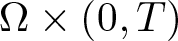 $\Omega\times (0,T)$, which is the first claim.
To show the second claim, assume first that  $x_0 = 0 \in \partial \Omega$. Let
 $\eta \in (0,\min\{1,T^{\beta}\})$ and define
 $w_\eta$ and
 $\Omega_\eta$ by
 \begin{equation*} w_\eta(x,t) :=\eta^{\frac{1 +\gamma}{1-q}}w(\eta^{-1/2}x,\eta^{-1}t), \quad \Omega_\eta:= \sqrt{\eta} \Omega \end{equation*}
which satisfy
 \begin{equation*}
\begin{cases}
\partial_t w_\eta-\Delta w_\eta \leq
k t^{\gamma}(w_\eta)^q &\text{in }\Omega_\eta\times (0,+\infty),\\
w_\eta \gt 0 & \text{in } \Omega_\eta\times (0,+\infty), \\
w_\eta=0 & \text{on }\partial \Omega_\eta\times (0,+\infty),\\
w_\eta=0& \text{on } \Omega_\eta \times \{0\}.
\end{cases}
\end{equation*}
Noticed that  $\Omega_{\eta} \subset \Omega$, by Proposition A.1 we obtain
 $u\geq w_\eta$ in
 $\overline{\Omega}_\eta\times (0,T)$. Now let
 $t=\eta^{\frac{1}{\beta}} \in (0, T)$ and, observed
 $0 \in \partial \Omega_{\eta}$, we choose
 $x=t\nu \in \Omega_{\eta}$ (i.e.
 $t^{1-\frac{\beta}{2}} \nu \in \Omega$ for
 $t$ small), so that
 \begin{equation}
u(t\nu,t^{\beta})\geq t^{\frac{\beta (1+\gamma)
}{1-q}}w(t^{\frac{2-\beta}{2}}\nu,1).
\end{equation}
If  $\beta=2$, we need a correction
 $rt \nu \in \Omega_{\eta}$ for
 $r$ small (so that
 $r \nu \in \Omega$), and the above expression becomes
 $u(r t \nu, (rt)^{2})\geq t^{\frac{2 (1+\gamma)
}{1-q}}w(r\nu,r^2)$ and the claim follows choosing
 $\delta := r^{-\frac{2 (1+\gamma)}{1-q}}w(r \nu, r^2)$. If
 $\beta \in (0,2)$, by Lagrange theorem there exists
 $\xi_{t}\in (0,t^{\frac{2-\beta}{2}}\nu)$ such that (recall
 $w(0,1)=0$)
 \begin{equation*}w(t^{\frac{2-\beta}{2}}\nu,1) = t^{\frac{2-\beta}{2}}\nu\cdot D_{x} w(\xi_t,1).
\end{equation*}
Being  $\delta:= \frac{1}{2}\nu\cdot D_{x} w(0,1) \gt 0$ thanks to Lemma A.4, for
 $t$ small enough we have
 $\nu\cdot D_{x} w(\xi_t,1) \gt \delta$ and hence we obtain
 \begin{equation}
w(t^{\frac{2-\beta}{2}}\nu,1) \geq \delta t^{\frac{2-\beta}{2}}\quad \hbox{for}\ t\ \hbox{small}.
\end{equation}
Thus, by (5.10) and (5.11) we obtain  $u(t\nu,t^{\beta})\geq \delta t^{\frac{2\beta(1+\gamma)+(2-\beta)(1-q) }{2(1-q)}}$.
The case of general  $x_0$ can be obtained straightforwardly, noticed that the equation related to
 $u \mapsto k t^{\gamma} u^q$ is
 $x$-translation invariant.
In the following proposition, we rule out the possibility of the negative minimum to be on the boundary of  $\Omega$ or at the initial time.
Proposition 5.12 (Rule out $\partial \Omega$ and $t=0$)


Let  $\Omega$ satisfy (5.3), and
 $u$ be such that (5.4), (5.5) and (5.6) hold. Let
 $v$ be as in (5.7). Suppose
 $b\colon\Omega\times(0,+\infty)\times (0,+\infty)\to \mathbb{R}$ is such that
 $b(x,\cdot,t)$ is differentiable for all
 $(x,t)\in \Omega\times (0,+\infty)$ and satisfies (H1), and let
 $\alpha \in \big(0, \frac{2(1-q)}{2\beta(1+\gamma)+(2-\beta)(1-q)}\big)$ and
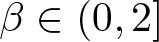 $\beta \in (0,2]$. Then
 $\mathcal{C}_{v}
$ cannot achieve any negative minimum at
 $(x_1,x_3,t_1,t_3,\lambda)\in \overline{\Omega} \times \overline{\Omega} \times [0,+\infty)\times [0,+\infty)\times (0,1) $ such that one of
 $t_1,t_3\in \left\{0\right\}$, or one of
 $x_1,x_2,x_3\in \partial \Omega$.
Proof. Assume now by contradiction that  $\mathcal{C}_{v}
$ admits a negative minimum at
 $(x_1,x_3,t_1,t_3,\lambda)$ such that one of
 $t_1,t_3\in \left\{0\right\}$ or one of
 $x_1,x_2,x_3\in \partial \Omega$. If
 $t_1,t_3\in [0,+\infty)$ and
 $x_1,x_3\in \partial \Omega$, then
 $\mathcal{C}_v(x_1,x_3,t_1,t_3,\lambda)=v(x_2,t_2) \geq 0$, which is not possible. If
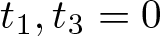 $t_1,t_3=0$ and
 $x_1,x_3\in \overline{\Omega}$,
 $\mathcal{C}_v(x_1,x_3,t_1,t_3,\lambda)= 0$ which again is not possible.
If  $t_1,t_3\in (0,+\infty)$,
 $x_1\in \partial \Omega$ and
 $x_3\in \Omega$, the parabolic Hopf Lemma A.4 implies
 $D_{\bar{\nu}_1}u (x_1, t_1^{\beta}) \gt 0$, where
 $\nu_1$ is the interior normal at
 $(x_1,t_1)$ and
 $\bar{\nu}_1:=(\tilde{\nu}_1, \beta t_1^{\beta-1}\nu_1^{n+1})$ thus
 \begin{align*}
& \lim_{(y_1,y_3,\tau_1,\tau_3,\eta)\to(x_1,x_3,t_1,t_3,\lambda)} D_{\nu_1}\mathcal{C}_v(y_1,y_3,\tau_1,\tau_3,\eta)\\ & \qquad =\lim_{(y_1,y_3,\tau_1,\tau_3,\eta)\to(x_1,x_3,t_1,t_3,\lambda)}\bigg((1-\eta) D_{\nu_1}v(y_2,\tau_2)-(1-\eta)\alpha u^{\alpha-1}(y_1,\tau_1^{\beta})\\
& \qquad\quad D_{\bar{\nu}_1} u(y_1, \tau_1^{\beta}) \bigg)=-\infty,
\end{align*}
and this is a contradiction since it is a minimum point. The same argument holds if  $t_1\in (0,+\infty)$,
 $t_3=0$,
 $x_1\in \partial \Omega$,
 $x_3\in \Omega$.
If  $t_1=0$,
 $t_3\in (0,+\infty)$,
 $x_1\in \Omega$ and
 $x_3\in \Omega$, by Lemma 5.11 (i) we have
 \begin{equation*}\limsup
_{\tau \to 0} v_t(x_1,\tau)\geq \limsup
_{\tau \to 0} \frac{v(x_1, \tau)}{\tau} \geq
C^{\alpha} \lim_{\tau \to 0} \frac{e^{-\alpha \lambda_1 \tau^{\beta}}}{\tau^{1-\frac{1+\gamma}{1-q}\alpha \beta}} (\varphi_{1}(x_1))^{\alpha} = +\infty\end{equation*}
by the assumption  $\alpha \lt \frac{2(1-q)}{2\beta(1+\gamma)+(2-\beta)(1-q)} \leq \frac{1-q}{\beta(1+\gamma)}$, which implies
 \begin{equation*}\lim_{(y_1,y_3,\tau_1,\tau_3,\eta)\to(x_1,x_3,t_1,t_3,\lambda)} D_{t_1}\mathcal{C}_v(y_1,y_3,\tau_1,\tau_3,\eta)=-\infty\end{equation*}
along a subsequence, again a contradiction.
We are left with the case  $t_1=0$,
 $t_3\in (0,+\infty)$,
 $x_1\in \partial \Omega$,
 $x_3 \in \Omega$. By Lemma 5.11 (ii) there exists
 $\delta \gt 0$ such that
 \begin{equation*}\frac{u^\alpha(x_1 +t\nu , t^{\beta})}{t}\geq \delta^\alpha t^{\alpha \frac{2\beta(1+\gamma)+(2-\beta)(1-q) }{2(1-q)} -1}\quad \hbox{for}\ t \gt 0\ \hbox{small},\end{equation*}
which positively diverges as  $t\to 0^+$ since
 $\alpha \lt \frac{2(1-q)}{2\beta(1+\gamma)+(2-\beta)(1-q)}$ by assumption. Thus
 $(\nu, 1) \cdot D_{(x_1, t_1)}\mathcal{C}_v$ negatively diverges while approaching
 $(x_1,t_1)$ and this implies
 $(x_1,x_3,t_1,t_3,\lambda)$ cannot be a minimum.
To deal with the case  $t=\infty$ we need to be able to compare the evolutive problem with the stationary one, and to this aim we will exploit the stability condition in Definition 3.2. From now on with
 $\widetilde{\mathscr{B}}(x,s,\tilde{p},\infty)$ and
 $v(x,\infty)$ we mean their pointwise limit in time whenever the stability condition is assumed.
Consider  $\alpha\in(0,1)$ and
 $\beta \in (0,2]$. In the following two remarks we discuss the possible localization of the global minimum of
 $\mathcal{C}_v$, in particular for
 $(t_1, t_3) \in [0,+\infty) \times \{+\infty\}$ and
 $\lambda\in \{0,1\}$.
Remark 5.13 (Case $(t_1, t_3) \in [0,+\infty) \times \{+\infty\}$)

Assuming  $v_t\geq 0$ in
 $\Omega \times (0,+\infty)$ and
 $v(x,t)\to v(x,\infty) \lt +\infty$ as
 $t\to+\infty$, if
 $(x_1,x_3,t_1,t_3,\lambda)\in \overline{\Omega}\times \overline{\Omega}\times [0,+\infty)\times \left\{+\infty\right\}\times (0,1)$ is a global minimum for
 $\mathcal{C}_v$, then also
 $(x_1,x_3,+\infty,+\infty,\lambda)$ is a global minimum for
 $\mathcal{C}_v$. Indeed
 \begin{align*}
\mathcal{C}_v(x_1,x_3,t_1,t_3,\lambda)&=v(x_2,\infty)-\lambda v(x_3,\infty
)-(1-\lambda)v(x_1,t_1
)\\
&\geq v(x_2,\infty)-\lambda v(x_3,\infty)-(1-\lambda)v(x_1,\infty).
\end{align*}
Remark 5.14 (Case $\lambda \in \{0,1\}$)

Let us discuss the case when  $\lambda\in\left\{0,1\right\}$. Assume
 $v_t\geq 0$ in
 $\Omega \times (0,+\infty)$ and
 $v(x,t)\to v(x,\infty) \lt +\infty$ as
 $t\to+\infty$. If
 $t_1,t_3\in [0,+\infty)$, then
 $\mathcal{C}_{v}
= 0$. If
 $t_3=+\infty$ and
 $\lambda=1$, then
 $\mathcal{C}_{v}
= 0$. If
 $\lambda = 0,t_3=+\infty$ let us consider a minimizing sequence
 $(x_1^n,x_3^n,t_1^n,t_3^n,\lambda^n)$ converging to
 $(x_1,x_3,t_1,+\infty,0)$ where
 $(x_1,x_3,t_1)\in\overline{\Omega}\times \overline{\Omega}\times [0,+\infty]$. We can assume, up to a subsequence, that
 $t_2^n$ converges to
 $t_2\in[t_1,+\infty]$. Since
 $x_2^n$ tends to
 $x_1$, then
 \begin{align*}
\lim_{n\to +\infty}\mathcal{C}_v(x_1^n,x_3^n,t_1^n,t_3^n,\lambda^n)&=v(x_1,t_2)-v(x_1,t_1)\geq 0.
\end{align*}
In light of Remarks 5.13 and 5.14, we will use the following convention.
Convention. If  $v_t\geq 0$, then by a global point of minimum for
 $\mathcal{C}_v$ on
 $\overline{\Omega}\times \overline{\Omega}\times [0,+\infty]\times [0,+\infty]\times [0,1]$ we mean a point picked in
 $\big(\overline{\Omega}\times \overline{\Omega}\times [0,+\infty)\times [0,+\infty) \times [0,1] \big) \cup \big(\overline{\Omega}\times \overline{\Omega}\times \{+\infty\}\times \{+\infty\}\times (0,1) \big)$.
With the above notations and conventions, and with the parabolic stability condition at hand, we can now include the case  $t=+\infty$ in the reasoning of Proposition 5.12.
Proposition 5.15. (On the case $t=+\infty$)

Under the same assumptions of Proposition 5.12, assume moreover  $v_t\geq 0$ and that
 $b$ satisfies the parabolic stability condition (e.g. i)–iv) in Remark 3.3 hold). Then
 $\mathcal{C}_{v}
$ cannot achieve any negative minimum at
 $(x_1,x_3,t_1,t_3,\lambda)\in \overline{\Omega} \times \overline{\Omega} \times [0,+\infty]\times [0,+\infty]\times (0,1) $ such that one of
 $t_1,t_3\in \left\{0\right\}$, or one of
 $x_1,x_2,x_3\in \partial \Omega$.
Proof. In light of Proposition 5.12 and Remark 5.13, we need to exclude only the stationary case  $t_1=t_3=+\infty$ and
 $x_1\in\partial \Omega$,
 $x_3\in \overline{\Omega}$; this can be done as in the proof of Proposition 5.12. See also [Reference Bucur and Squassina13, Reference Kennington49].
By knowing the behaviour of the concavity function on the boundary, we are now able to deduce the main concavity estimate of this section.
Theorem 5.16 (Estimate on power-concavity)
Let  $\Omega$ satisfy (5.3), and
 $u$ be a function such that (5.4), (5.5) and (5.6) hold. Let
 $\beta \in [1,2]$ and suppose
 $b\colon\Omega\times(0,+\infty)\times (0,+\infty)\to \mathbb{R}$ is such that
 $b(x,\cdot, t) \in C^1((0,+\infty))$ for all
 $(x,t)\in \Omega \times (0,+\infty)$, (H1), (H2) (with
 $T=\infty$) hold and
(i)
$\partial_s \left(s^{\alpha-1}b(x,s, t)\right) \lt 0$ for all $(x,s,t)\in \Omega \times (0,+\infty) \times (0,+\infty)$ for some $\alpha \in (0,1)$ as in Proposition 5.12.(ii)
$b$ satisfies the parabolic stability condition (e.g. i)–iv) in Remark 3.3 hold).(iii)
$b(x, s, \cdot)$ is nondecreasing for each $(x,s) \in \Omega \times (0,+\infty)$.


Then  $u_t \geq 0$. Let
 $(x_1,x_3,t_1,t_3,\lambda)\in \overline{\Omega}\times \overline{\Omega}\times [0,+\infty]\times [0,+\infty]\times [0,1]$ be a global minimum for
 $\mathcal{C}_{u^\alpha(\cdot, \star^{\beta})}
$ (with the above convention). Then (4.10) holds true for some
 $\sigma \gt 0$ and
 \begin{equation*}
\min_{\overline{\Omega}\times \overline{\Omega}\times[0,+\infty]\times [0,+\infty]\times[0,1]}\mathcal{C}_{u^\alpha(\cdot, \star^{\beta})} \geq -\frac{1}{\sigma}\mathcal{HC}^-_{\widetilde{\mathscr{B}}(\cdot, u^\alpha(\cdot,\star^{\beta}),D_xu^\alpha(x_1,t_1^{\beta}), \star)}(x_1,x_3,t_1,t_3,\lambda).
\end{equation*}
Proof. By (H2) we can apply Corollary A.3 and obtain  $u_t\geq 0$ in
 $ \Omega\times (0,+\infty)$, which in turn implies
 $v_t\geq 0$ (so we are in the setting of the above convention). If the minimum is nonnegative, the statement holds.
Assume
 $\mathcal{C}_{u^\alpha(\cdot, \star^{\beta})}$ admits a negative minimum.
By Remark 5.14 and Proposition 5.15, we know that
 $(x_1,x_3,t_1,t_3,\lambda)\in \Omega\times \Omega\times (0,+\infty]\times (0,+\infty]\times (0,1)$.
Let us verify the hypotheses of Corollary 4.5 on the equation (5.8) satisfied by  $v$. The function
 $\mathscr{B}$ takes the form (5.9).
Since
 $\alpha^{-1}(1-\alpha)s^{-1}|\tilde{p}|^2$ is nonincreasing with respect to
 $s$,
 $(i)$ implies the existence of
 $\sigma \gt 0$ such that (4.10) holds.
If  $(x_1,x_3,t_1,t_3,\lambda)\in \Omega\times \Omega\times (0,+\infty)\times (0,+\infty)\times (0,1)$, then the claim follows by Corollary 4.5.
If
 $t_1=t_3=+\infty$ the claim follows by [Reference Bucur and Squassina13, Lemma 2.9]. We conclude by observing that, being
 $\beta \in [1,2]$, we have
 $\mathcal{HC}_{\star^{1-\beta}} \leq 0$.
In the following corollary, starting from Theorem 5.16, we deduce a bound in terms of the concavity function of the nonlinearity (rather than on the harmonic function).
Corollary 5.17. In the assumptions of Theorem 5.16, we also have
 \begin{equation*} \min_{\overline{\Omega}\times \overline{\Omega}\times[0,+\infty]\times [0,+\infty]\times[0,1]}\mathcal{C}_{u^\alpha(\cdot, \star^{\beta})} \geq-\frac{\alpha}{\sigma}\frac{\mathcal{C}^-_{\tilde{g}(\cdot, u^{\alpha}(\cdot,\star^{\beta}), \star)}(x_1,x_3,t_1,t_3,\lambda)}{(\lambda u^\alpha(x_3,t_3^{\beta})
+(1-\lambda)u^\alpha(x_1,t_1^{\beta}))^2}\end{equation*}
where  $\tilde{g}(x,s,t):= s^{\frac{3\alpha-1}{\alpha}}b(x,s^{1/\alpha}, t^{\beta})$.
Proof. Since Theorem 5.16 holds, let us give a lower bound for the  $\mathcal{HC}^-_{\widetilde{\mathscr{B}}}$. Set
 \begin{equation*}g(x,s, t):=s^2\widetilde{\mathscr{B}}(x,s,\tilde{\xi},t)= \frac{1-\alpha}{\alpha}|\tilde{\xi}|^2s+\alpha s^{\frac{3\alpha-1}{\alpha}}b(x,s^{1/\alpha}, t^{\beta})\end{equation*}
where  $\tilde{\xi}=
D_x u^{\alpha}(x_1, t_1^{\beta})$, and moreover
 $v(x,t) = u^{\alpha}(x,t^{\beta})$.
By Proposition B.3 we have
 \begin{align*}
& {\mathcal{HC}}_{\widetilde{\mathscr{B}}(\cdot,v(\cdot,\star),\tilde{\xi}, \star)}(x_1,x_3,t_1,t_3,\lambda)\geq\frac{\mathcal{C}_{g(\cdot,v(\cdot,\star), \star)}(x_1,x_3,t_1,t_3,\lambda)}{(\lambda v_3 +(1-\lambda)v_1 )^2}.
\end{align*}
Since  $\frac{1-\alpha}{\alpha}|\tilde{\xi}|^2s$ is linear we have
 $\mathcal{C}_g=\alpha\mathcal{C}_{\tilde{g}(\cdot, v(\cdot, \star), \star)}$ and hence
 \begin{equation*} \mathcal{HC}_{\widetilde{\mathscr{B}}(\cdot,v(\cdot,\star),\tilde{\xi}, \star)}(x_1,x_3,t_1,t_3,\lambda)\geq \alpha\frac{\mathcal{C}_{\tilde{g}(\cdot, v(\cdot, \star), \star) }(x_1,x_3,t_1,t_3,\lambda)}{(\lambda v_3 +(1-\lambda)v_1 )^2} \end{equation*}
and thus the claim.
As a consequence of Corollary 5.17, we obtain the following result.
Corollary 5.18 (Exact power-concavity)
In the assumptions of Theorem 5.16, assume moreover
iv)
$(x,s,t) \mapsto s^{\frac{3\alpha-1}{\alpha}}b(x,s^{\frac{1}{\alpha}},t^{\beta}) $ is a concave function.

Then  $u^\alpha(\cdot, \star^{\beta})$ is a concave function in
 $\overline{\Omega}\times [0,+\infty]$.
5.2.1. Applications
Let  $\Omega$ be a convex bounded domain of
 $\mathbb{R}^n$ and suppose
 $u$ is a function such that (5.4) and (5.6) hold together with (5.5) in the case
 $b(x,u,t)=a(x,t) u^q$, namely
 \begin{equation}
u_t-\Delta u=a(x,t)u^q \quad\text{in }\Omega\times (0,+\infty),
\end{equation}
where  $q\in[0,1)$ and
 $a\colon\Omega \times (0,+\infty)\to \mathbb{R}$ is such that
 $a(\cdot,t)$ is measurable for all
 $t\in(0,+\infty)$.
Let us start from some exact results. For the sake of simplicity, we focus on  $a(x,t)=a(x) t^{\gamma}$, but more general behaviours in time may be considered.
Proof of Theorem 1.3
Let us verify the hypotheses of Corollary 5.18 with
 \begin{equation*}\alpha= \frac{\theta(1-q)}{1+2\theta +\beta \gamma \theta} \lt \frac{2(1-q)}{2\beta(1+\gamma)+(2-\beta)(1-q)} \lt 1-q\end{equation*}
and  $b(x,s, t)=a(x) t^{\gamma} s^q$. Notice
 $s \mapsto s^{\alpha-1} b(x,s,t) = a(x) t^{\gamma} s^{\alpha-(1-q)}$ is strictly decreasing for all
 $x\in \Omega$ and
 $t \gt 0$. Moreover
 $s \mapsto s^{\frac{3\alpha -1}{\alpha}}b(x,s^{1/\alpha},t^{\beta})=a(x) t^{\gamma \beta} s^{3-\frac{1-q}{\alpha}} $ is concave as a product since
 $\frac{1}{\theta}+\beta \gamma + 3-\frac{1-q}{\alpha}=1$, by the assumptions we have
 $3-\frac{1-q}{\alpha}\geq 0$ and thus the claim in light of Proposition 3.9 (iv). To get the parabolic condition, we argue as in Remark 3.6 (notice that the solution of the stationary problem of
 $-\Delta u = a(x) u^q$ is
 $\frac{\theta(1-q)}{1+2\theta}$-concave, where
 $\frac{\theta(1-q)}{1+2\theta}\geq \frac{\theta(1-q)}{1+2\theta +\beta \gamma \theta}$) thanks to Remark 3.3, while we see that (H2) is satisfied as shown in Remark 3.4. Then we can apply Corollary 5.18 and get the thesis. Moreover if
 $a$ is a constant, then
 $a$ is
 $\theta$-concave for all
 $\theta\geq 1$, thus the claim by Proposition 3.9 (ii). Finally, we see that, if
 $\beta=\frac{1}{\gamma}\leq 2$ and
 $a$ is constant, we can repeat the previous arguments with
 $\alpha=\frac{1-q}{2+\beta \gamma }$ and obtain the claim.
Proof of Theorem 1.4
Let us verify that  $b(x, s)=a(x) s^p+s^q$ satisfies the hypotheses of Corollary 5.18 with
 $\alpha=\frac{1-q}{2}$. Since
 $s^{\frac{1-q}{2}-1}(a(x) s^p+s^q)=a(x) s^{\frac{-1-q+2p}{2}}+s^{\frac{q-1}{2}}$, it is strictly decreasing by the hypothesis on
 $p$. Moreover the parabolic stability condition is guaranteed by Remark 3.3 and
 $b(x, s)=a(x) s^p+s^q$ satisfies (H2) as shown in Remark 3.4. Regarding the concavity, we observe that
 $s \mapsto a(x) s^{\frac{1-3q+2p}{1-q}} +s$ is concave by the assumptions. Thus we have the claim.
Proposition 5.19. Let  $\Omega$ satisfy (5.3), and
 $u$ be a function such that (5.4) and (5.6) hold. Suppose
 \begin{equation*}
u_t-\Delta u= (1-u)^p \quad\textit{in }\Omega\times (0,+\infty)
\end{equation*}
for some  $p\in (0,1)$. Then
 $u(\cdot, \star^{2})$ is
 $\frac{1}{2}$-concave in
 $\overline{\Omega} \times [0,+\infty)$.
Proof. Notice that  $u(\Omega \times (0,+\infty)) \subset [0,1]$; thus, we can substitute the right-hand side with
 $u$
 $(1-s)^p \chi_{[0,1]}(s)$ with
 $s \in \mathbb{R}$ (notice that the derivative explodes to
 $-\infty$ in
 $s=1$; anyway, for exact concavity arguments, it is sufficient a strict monotonicity on the image of
 $u$). Observe that
 $b(s)=(1-s)^p$ satisfies (H2) (being nonincreasing), and it satisfies (H1) with
 $q=0$ for
 $M \lt 1$. To conclude it is sufficient to observe that
 $s^{\alpha-1} b(s)$ is strictly decreasing for each
 $\alpha \in (0,1)$, while
 $s^{\frac{3\alpha-1}{\alpha}}b(s^{\frac{1}{\alpha}})$ is concave for each
 $\alpha \in [\frac{1}{3}, \frac{1}{2}]$. Noticed that
 $\alpha \lt \frac{1}{2} $ satisfies the restriction of Proposition 5.12, then the claim holds by Corollary 5.18 for such
 $\alpha$; by continuity of power concavity (see Proposition 3.9), the claim holds also for
 $\alpha=\frac{1}{2}$.
Remark 5.20. In [Reference Kennington48] the author shows that, for  $\beta=1$, the solution
 $u$ is such that
 $\varphi_p(u)$ is concave, where
 $\varphi_p(s) := \int_0^s \frac{1}{\sqrt{1-(1-r)^{p+1}}
} dr$. Set
 $\psi(s):=\sqrt{s}$ the transformation found in Proposition 5.19, by the fact that
 $\psi \circ \varphi_p^{-1}$ is (strictly) concave, we see that, generally, the information given by
 $\varphi_p$ is better (when compared to
 $\beta=1$). This fact is due to the choice of a transformation not necessarily of power type, but tailored on the nonlinearity, that is, up to constants,
 $\varphi_p(s)=\int_0^{s} \frac{1}{\sqrt{F(r)}} dr$, where
 $F(s)=\int_0^{s} f(r) dr$,
 $f(s)=(1-s)^p$. This choice is coherent with the approach in [Reference Almousa, Assettini, Gallo and Squassina2, Reference Borrelli, Mosconi and Squassina11, Reference Gallo and Squassina32]. In the present paper, we decided not to pursue this approach in order to focus on the difficulties given by the parabolic framework and avoid technicalities. On the other hand, similar arguments could be developed, and we leave the details to the interested reader.
Let us now move to some perturbative result for (5.12). For the sake of simplicity, we consider  $a=a(x)$ locally bounded (see also Remark 5.25), and
 $\beta=1$.
Let  $(x_1,x_3,t_1,t_3,\lambda)\in \Omega\times \Omega \times (0,+\infty]\times (0,+\infty]\times (0,1)$ be a global interior minimum of
 $\mathcal{C}_{u^{\frac{1-q}{2}}}$, then by (4.9) in Theorem 4.4 (and [Reference Kennington49]) we have
 \begin{align*}\tilde{\xi} & :=\tfrac{1-q}{2} u^{-\frac{1+q}{2}}(x_1,t_1)D_xu(x_1,t_1)=\tfrac{1-q}{2} u^{-\frac{1+q}{2}}(x_2,t_2)D_xu(x_2,t_2)\\ & =\tfrac{1-q}{2} u^{-\frac{1+q}{2}}(x_3,t_3)D_xu(x_3,t_3).\end{align*}
We define, for any  $\rho \gt 0$ small enough,
 \begin{equation}
\mathfrak{m}_{\rho} :=\frac{2}{1-q} \inf_{x \in \overline{\Omega_{\rho}}}f^{\tilde{\xi}}(x) ,\quad \mathfrak{M}_{\rho} :=\frac{2}{1-q} \sup_{x \in \overline{\Omega_{\rho}}}f^{\tilde{\xi}}(x),
\end{equation}
where
 \begin{equation}
f^{\tilde{p}}(x):=\dfrac{1+q}{1-q}|\tilde{p}|^2+\dfrac{1-q}{2}a(x), \quad \hbox{for}\ \tilde{p} \in \mathbb{R}^n\ \hbox{and}\ x \in \Omega.
\end{equation}
Notice that
 \begin{equation}
\mathfrak{M}_{\rho} - \mathfrak{m}_{\rho} = \sup _{\overline{\Omega_{\rho}} } a - \inf_{\overline{\Omega_{\rho}}} a, \quad \mathfrak{m}_{\rho} \geq \inf_{\overline{\Omega_{\rho}}} a.
\end{equation}
Proposition 5.21 (Oscillation estimate)
Let  $\Omega$ satisfy (5.3), and
 $u$ be a function such that (5.4), (5.6) and (5.12) hold. Suppose moreover
 $a\colon\Omega \to \mathbb{R}$ measurable, bounded and
 $a\geq m \gt 0$. Then
 $u$ is increasing in time and there exists
 $\rho \gt 0$ such that
 \begin{equation*}
\min_{\overline{\Omega}\times \overline{\Omega}\times[0,+\infty]\times [0,+\infty]\times[0,1]}\mathcal{C}_{u^{\frac{1-q}{2}}}\geq
- \frac{\|u(\cdot, \infty)\|^{\frac{1-q}{2}}_{L^{\infty}(\overline{\Omega})}}{\mathfrak{m}_{\rho} } \left(\inf_{\overline{\Omega_\rho}\times \overline{\Omega_\rho} \times [0,1] } \mathcal{C}_{a}-\frac{\mathfrak{M}_{\rho} }{\mathfrak{m}_{\rho} }\varepsilon \right)^{-}.
\end{equation*}
where  $\varepsilon:= \mathfrak{M}_{\rho} - \mathfrak{m}_{\rho} \geq 0$ and
 $ \mathfrak{M}_{\rho} , \mathfrak{m}_{\rho} $ are defined in (5.13). In particular
 \begin{equation*}\min_{\overline{\Omega}\times \overline{\Omega}\times[0,+\infty]\times [0,+\infty]\times[0,1]}\mathcal{C}_{u^{\frac{1-q}{2}}} \geq
-\|u(\cdot, \infty)\|^{\frac{1-q}{2}}_{L^{\infty}(\overline{\Omega_{\rho}})} \left(2+ \frac{\varepsilon }{\inf_{\overline{\Omega_{\rho}}} a} \right) \frac{\varepsilon}{\inf_{\overline{\Omega_{\rho}}} a } .\end{equation*}
Proof. We want to apply Theorem 5.16 with  $\alpha= \frac{1-q}{2}
$ and
 $b(x,s)=a(x)s^q$. Since
 $a$ is bounded from below,
 $b(x,s)\geq m s^q$. Moreover
 $s^{\alpha-1}b(x,s)=s^{\frac{1-q}{2}-1}a(x)s^q=a(x)s^{\frac{q-1}{2}}$ is a strictly decreasing function of
 $s$, the parabolic condition on
 $b$ is satisfied by Remark 3.3 and (H2) is satisfied as shown in Remark 3.4. Thus we can apply Theorem 5.16. Notice that
 $\widetilde{\mathscr{B}}$ defined in (5.9) takes the form
 \begin{equation*}\widetilde{\mathscr{B}}(x,s,\tilde{p})=\dfrac{f^{\tilde{p}}(x)}{s}\end{equation*}
where  $f^{\tilde{p}}$ is given in (5.14). Let
 $(x_1,x_3,t_1,t_3,\lambda)\in \overline{\Omega}\times \overline{\Omega}\times [0,+\infty]\times [0,+\infty]\times [0,1]$ be a global minimum for
 $\mathcal{C}_{v}$. By Proposition 5.15, we know that
 $(x_1,x_3,t_1,t_3,\lambda)\in \Omega\times \Omega\times (0,+\infty]\times (0,+\infty]\times [0,1]$. If the minimum is nonnegative, the statement holds. Suppose
 $\mathcal{C}_{v}$ admits a negative minimum at
 $(x_1,x_3,t_1,t_3,\lambda)\in \Omega\times \Omega\times (0,+\infty)\times (0,+\infty)\times (0,1)$, then we need to estimate the harmonic concavity function. Define
 \begin{equation*}\rho:=\min \big\{d(x_1,\partial\Omega),d(x_3,\partial \Omega)\big\} \gt 0. \end{equation*}
Then by (5.13), it holds (recall (3.6))
 \begin{align*}
& {\mathcal{HC}}_{\widetilde{\mathscr{B}}(\cdot,v(\cdot,\star),\tilde{\xi})}(x_1,x_3,t_1,t_3,\lambda)\\
= & \dfrac{f^{\tilde{\xi}}_2}{\lambda v_3 +(1-\lambda)v_1}-\dfrac{f^{\tilde{\xi}}_1}{v_1}\dfrac{f^{\tilde{\xi}}_3}{v_3 }\dfrac{v_1 v_3 }{\lambda f^{\tilde{\xi}}_1 v_3 +(1-\lambda)f^{\tilde{\xi}}_3v_1}\\
=& \dfrac{1}{\lambda v_3 +(1-\lambda)v_1}\left( f^{\tilde{\xi}}_2-f^{\tilde{\xi}}_1f^{\tilde{\xi}}_3\dfrac{\lambda v_3 +(1-\lambda)v_1}{\lambda f^{\tilde{\xi}}_1 v_3 +(1-\lambda)f^{\tilde{\xi}}_3v_1}\right)\\
\geq & \dfrac{1}{\lambda v_3 +(1-\lambda)v_1} \left(\mathcal{HC}_{f^{\tilde{\xi}}}(x_1,x_3,\lambda
)+f^{\tilde{\xi}}_1f^{\tilde{\xi}}_3\left(\frac{1}{\lambda f^{\tilde{\xi}}_1+(1-\lambda)f^{\tilde{\xi}}_3}-\frac{2}{(1-q) \mathfrak{m}_{\rho} } \right)\right) \\
\geq & \dfrac{1}{\lambda v_3 +(1-\lambda)v_1} \left(\mathcal{HC}_{f^{\tilde{\xi}}}(x_1,x_3,\lambda
)+\frac{1-q}{2} \mathfrak{M}_{\rho} ^2\left(\frac{1}{\mathfrak{M}_{\rho} }-\frac{1}{\mathfrak{m}_{\rho} } \right)\right) \\
\geq & \dfrac{1}{\lambda v_3 +(1-\lambda)v_1} \left(\mathcal{C}_{f^{\tilde{\xi}}}(x_1,x_3,\lambda
)-\frac{1-q}{2}\frac{\mathfrak{M}_{\rho} }{\mathfrak{m}_{\rho} }( \mathfrak{M}_{\rho} - \mathfrak{m}_{\rho} )\right)\\
= & \frac{1-q}{2}\dfrac{1}{\lambda v_3 +(1-\lambda)v_1} \left(\mathcal{C}_{a}(x_1,x_3,\lambda
)-\frac{\mathfrak{M}_{\rho} }{\mathfrak{m}_{\rho} }\varepsilon\right).
\end{align*}
In the case  $t_1=+\infty$ or
 $t_3=+\infty$, the previous inequality holds by the same arguments for
 $\mathcal{HC}_{\widetilde{\mathscr{B}}(\cdot,v(\cdot,\star),\tilde{\xi})}(x_1,x_3,+\infty,+\infty,\lambda)$. Thus it holds
 \begin{equation*} \mathcal{HC}_{\widetilde{\mathscr{B}}(\cdot,v(\cdot,\star),\tilde{\xi})}(x_1,x_3,+\infty, +\infty,\lambda)
\geq
\frac{1-q}{2} \frac{1}{\lambda v_3 +(1-\lambda)v_1} \left(\mathcal{C}_{a}(x_1,x_3,\lambda)-\frac{\mathfrak{M}_{\rho} }{\mathfrak{m}_{\rho} }\varepsilon\right).\end{equation*}
Let us write explicitly the constant  $\sigma$ of (4.10) recalling that
 $ v_2 \lt \lambda v_3 +(1-\lambda)v_1$:
 \begin{align*}
\sup_{z\in [ v_2 ,\lambda v_3 +(1-\lambda)v_1]} \partial_s\widetilde{\mathscr{B}}(x_2,z,D_x v_2 ) & \leq f^{D_x v_2 }(x_2) \sup_{z\in [ v_2 ,\lambda v_3 +(1-\lambda)v_1]}\bigg(-\frac{1}{z^2}\bigg)
\\ &
\leq -\frac{1-q}{2}\frac{\mathfrak{m}_{\rho} }{(\lambda v_3 +(1-\lambda)v_1)^2}
\end{align*}
which leads to  $\sigma:=\frac{1-q}{2}\frac{\mathfrak{m}_{\rho} }{(\lambda v_3 +(1-\lambda)v_1)^2}$. Finally, by Theorem 5.16, it holds
 \begin{equation*}\min_{\overline{\Omega}\times \overline{\Omega}\times[0,+\infty]\times [0,+\infty]\times[0,1]}\mathcal{C}_{u^{\frac{1-q}{2}}}\geq
\min \left\{0,\frac{\lambda v_3 +(1-\lambda)v_1}{\mathfrak{m}_{\rho} } \left(\mathcal{C}_{a}(x_1,x_3,\lambda)-\frac{\mathfrak{M}_{\rho} }{\mathfrak{m}_{\rho} }\varepsilon\right)\right\}\end{equation*}
which implies the claim. We conclude by observing that  $\mathcal{C}_{a} \geq \inf_{\overline{\Omega_{\rho}}}
a - \sup_{\overline{\Omega_{\rho}}}
a$ on
 $\overline{\Omega_{\rho}}
$, (5.15) and the trivial identity
 $\frac{\mathfrak{M}_{\rho} }{\mathfrak{m}_{\rho}} = \frac{\mathfrak{M}_{\rho} - \mathfrak{m}_{\rho} }{\mathfrak{m}_{\rho}} +1$.
Remark 5.22. We highlight that, in the previous proof, we exploited  $\inf_{\Omega} a \gt 0$. On the other hand, with regard to the conclusion, we observe that if
 $a\to 0$ on
 $\partial \Omega$, the final expression is still well defined; we refer to Section 6 for some generalization for the torsion problem in this direction.
Assumed  $a$ bounded and set
 $M:= \sup_{\Omega} a,\ m:= \inf_{\Omega} a$, the final statement in Proposition 5.21 implies
 \begin{equation*}\min_{\overline{\Omega}\times \overline{\Omega}\times[0,+\infty]\times [0,+\infty]\times[0,1]}\mathcal{C}_{u^{\frac{1-q}{2}}} \geq
- \|u(\cdot, \infty)\|^{\frac{1-q}{2}}_\infty \left(2+ \frac{{\rm osc}(a) }{m} \right) \frac{{\rm osc}(a)}{m}\end{equation*}
where we recall  ${\rm osc}(a)=M-m$. Finally, if
 $a\in C^1(\Omega)$, it is possible to express
 $\varepsilon$ in terms of the gradient of
 $a$. Indeed for some
 $\bar{x},\tilde{x}\in\overline{\Omega_\rho}$ and
 $\bar{z}$ on the segment
 $[\bar{x},\tilde{x}]$ lying in
 $\overline{\Omega_\rho}$, it holds
 \begin{align*}
\varepsilon = \mathfrak{M}_{\rho} - \mathfrak{m}_{\rho} &= \nabla a (\bar{z}) \cdot (\bar{x}-\tilde{x})
\leq \|\nabla a\|_{\infty} {\rm diam} (\Omega).
\end{align*}
As a consequence of Proposition 3.10, Proposition 5.21 and Remark 5.22, we obtain the following result.
Corollary 5.23 (Hyers–Ulam approximation)
Under the assumptions of Proposition 5.21, there exist  $C=C\big(\|u(\cdot, \infty)\|_{\infty}, \inf_{\Omega} a, {\rm osc}(a), q,
n \big) \gt 0$ (with a linear dependence with respect to
 ${\rm osc}(a)$) and a concave function
 $w:\Omega\times(0,+\infty)\to \mathbb{R}$ such that
 \begin{equation*} \|u^{\frac{1-q}{2}}-w\|_{L^\infty(\Omega\times(0,+\infty))}\leq C {\rm osc}(a).\end{equation*}
Proposition 5.24 ($\theta$-concavity estimate)

Let  $\Omega$ satisfy (5.3),
 $\theta \geq 1$, and
 $u$ be a function such that (5.4), (5.6) and (5.12) hold. Suppose moreover
 $a\colon\Omega \to \mathbb{R}$ measurable,
 $0 \lt m\leq a\leq M$ and
 $m^\theta\geq M^{\theta}/2$. Let
 $(x_1,x_3,t_1,t_3,\lambda)\in \overline{\Omega}\times \overline{\Omega}\times [0,+\infty]\times [0,+\infty]\times [0,1]$ be a global minimum for
 $\mathcal{C}_{u^{\frac{\theta(1-q)}{1+2\theta}}}$. Then
 \begin{equation*} \min_{\overline{\Omega}\times \overline{\Omega}\times[0,+\infty]\times [0,+\infty]\times[0,1]}\mathcal{C}_{u^{\frac{\theta(1-q)}{1+2\theta}}}
\geq
-\frac{\theta }{1+\theta}\frac{||u(\cdot, \infty)||_{L^{\infty}(\Omega)}^{\frac{\theta(1-q)}{1+2\theta}}}{m}(\mathcal{C}^-_{a^{\theta}})^{1/\theta}(x_1,x_3,\lambda).
\end{equation*}
Proof. As in Proposition 5.21, the hypotheses imply Corollary 5.17. Being  $b(x,s)=a(x)s^q$, we need to evaluate
 $\mathcal{C}_{\tilde{g}(\cdot, v(\cdot, \star))}$ with
 $\tilde{g}(x,s):= a(x) s^{\frac{3\alpha-1+q}{\alpha}}$ and
 $\alpha=\frac{\theta(1-q)}{1+2\theta}$. We see that
 $s\mapsto s^{\frac{3\alpha-1+q}{\alpha}}$ is
 $\left(1-\frac{1}{\theta}\right)^{-1}$-concave. If
 $\theta \gt 1$, applying Proposition B.1 it holds
 \begin{align*}
\mathcal{C}_{\tilde{g}(\cdot, v(\cdot, \star))} (x_1,x_3,t_1,t_3,\lambda)\geq
& -(\mathcal{C}^-_{a^{\theta}})^{1/\theta}(x_1,x_3,\lambda) \big(\lambda v^{1-1/\theta}_3+(1-\lambda) v^{1-1/\theta}_1\big).
\end{align*}
If instead  $\theta=1$, the previous inequality is obvious. So by Corollary 5.17
 \begin{align*}
\mathcal{C}_{u^\alpha}(x_1,x_3,t_1,t_3, \lambda)
\geq&-\frac{\alpha}{\sigma}\frac{\mathcal{C}_{\tilde{g}(\cdot, v(\cdot, \star))}^-
(x_1,x_3,t_1,t_3,\lambda)}{(\lambda v_3
+(1-\lambda)v_1)^2}
\\\geq& -\frac{\theta(1-q)}{1+2\theta}\frac{1}{\sigma}\frac{(\lambda v^{1-1/\theta}_3+(1-\lambda) v^{1-1/\theta}_1)}{(\lambda v_3+(1-\lambda)v_1)^2}(\mathcal{C}^-_{a^{\theta}})^{1/\theta}(x_1,x_3,\lambda).
\end{align*}
Then as in Proposition 5.21, we give an estimate of  $\sigma$: since
 $\widetilde{\mathscr{B}}$ in (5.9) is given by
 \begin{equation*} \widetilde{\mathscr{B}}(x,s,\tilde{p},t) = \frac{1+\theta+\theta q}{\theta(1-q)}
\frac{|\tilde{p}|^2}{s}+\frac{\theta(1-q)}{1+2\theta} a(x) s^{-\frac{1+\theta}{\theta}}
\end{equation*}
we have (for the sake of simplicity, here we straightaway get rid of the  $\tilde{\xi}$-term)
 \begin{align*}
\sup_{z\in [v_2,\lambda v_3+(1-\lambda)v_1]} \partial_s\widetilde{\mathscr{B}}(x_2,z,\tilde{\xi},t_2) &= \partial_s\widetilde{\mathscr{B}}(x_2,\lambda v_3+(1-\lambda)v_1,\tilde{\xi},t_2) \\
&\leq -\frac{(1+\theta)(1-q)}{1+2\theta} a(x_2) \big(\lambda v_3+(1-\lambda)v_1\big)^{-\frac{1+2\theta}{\theta}}
\end{align*}
hence
 \begin{align*}
\mathcal{C}_{u^\alpha}(x_1,x_3,t_1,t_3, \lambda) &\geq -\frac{\theta(1-q)}{1+2\theta}\frac{1}{\sigma}\frac{(\lambda v^{1-1/\theta}_3+(1-\lambda) v^{1-1/\theta}_1)}{(\lambda v_3+(1-\lambda)v_1)^2}(\mathcal{C}^-_{a^{\theta}})^{1/\theta}(x_1,x_3,\lambda)\\
& \geq -\frac{\theta}{1+\theta} \frac{1}{a(x_2)} \big(\lambda v_3+(1-\lambda)v_1\big)^{\frac{1}{\theta}} (\lambda v^{1-1/\theta}_3+(1-\lambda) v^{1-1/\theta}_1)\\ &\quad \times (\mathcal{C}^-_{a^{\theta}})^{1/\theta}(x_1,x_3,\lambda) \\
& \geq -\frac{\theta}{1+\theta} \frac{1}{m} \|u\|_{\infty}^{\frac{\theta(1-q)}{1+2\theta}} (\mathcal{C}^-_{a^{\theta}})^{1/\theta}(x_1,x_3,\lambda).
\end{align*}
Proof of Theorem 1.6
It is a consequence of Proposition 5.24 (see also Remark 5.22).
Remark 5.25. The above perturbative results can also be extended to time-dependent nonlinearities  $a(x,t)$. If, for instance,
 $a(x,t)$ is bounded and
 $a(x,t)\to \bar{a}(x)$ as
 $t\to +\infty$, it makes sense to investigate the parabolic stability condition for
 $b$. Moreover, if
 $a \gt 0$ in
 $\Omega \times (0,+\infty)$, one can consider the infimum over
 $\Omega_{\rho} \times [\rho, +\infty)$, where
 $\rho:=\min \big\{d(x_1,\partial\Omega),d(x_3,\partial \Omega), t_1, t_3\big\} \gt 0$.
If instead  $a(x,t) \sim a(x) t^{\gamma}$, then one may consider a truncation argument (see Remark 3.6) so that
 $a$ becomes bounded. In such a case, anyway, the perturbative estimate will depend on
 $T$. We omit the details, and leave them to the interested reader.
Remark 5.26. (Comments on $u(\cdot, 0) \neq 0$)

In the whole Subsection 5.2, we considered only zero initial conditions  $u(\cdot, 0)=u_0=0$, in accordance to [Reference Ishige, Liu and Salani40, Reference Ishige and Salani42, Reference Ishige and Salani43, Reference Kennington48]. Many of our arguments, anyway, could also be adapted to nonzero initial conditions. First, assume, in place of (H1), the following slightly stronger assumption:
There exist  $T \gt 0$,
 $q\in [0,1)$ and
 $\gamma \in [0,1]$ such that for all
 $M \gt 0$ there exists
 $k=k(M,T) \gt 0$ verifying
 \begin{equation*}b(x,s, t)\geq k t^{\gamma} s^q \quad \hbox{for all}\ (x,s,t)\in \Omega\times(0,M]\times (0,T].\end{equation*}
As in (H2),  $\|u\|_{\infty}$ takes the place of
 $M$. Notice that
 $f(s)=(1-s)^p$ (studied in Proposition 5.19) satisfies (H1) but not (H1*).
Assume
- $u_0 \in C(\overline{\Omega})$, $u_0=0$ on $\partial\Omega$,
(5.16)\begin{equation}
u_0\geq \delta d_{\Omega} \quad \hbox{for some}\ \delta \gt 0,
\end{equation}$u_0$ is $\alpha$-concave for some (suitable) $\alpha$, and
(for instance, when (H3) holds, we can require\begin{equation*}u(\cdot, t)\geq u_0 \quad \hbox{for each}\ t \gt 0\end{equation*}$u_0$ to be a subsolution of the stationary problem, see Corollary A.3). We highlight that the set of functions satisfying these conditions is nonempty; for example, consider $\Omega = B_1$, $b(x,s,t)=a(x)\in L^\infty(\Omega)$ with $a\geq m \gt 0$; let $u_0(x)=\delta d_{\Omega}(x) =\delta(1-|x|)$, $\delta$ small enough, on $B_1\setminus B_{\frac{1}{2}}$ and extended smoothly and in a concave way to $B_{\frac{1}{2}}$; then $-\Delta u_0=\delta \frac{n
-1}{|x|}\leq a(x)$ in $B_1 \setminus B_{\frac{1}{2}}$ and we can require also $-\Delta u_0\leq a(x)$ in $B_{\frac{1}{2}}$; thus, $u_0$ satisfies all the assumptions ($\alpha=1$); less trivial examples (such as perturbations of the present examples) hold as well. Moreover the requirement (5.16) is related to the application of comparison principles, see Proposition A.1; by requiring more regularity on $b$ (see (H2*)), this condition can be dropped (see Proposition A.2).


All the arguments still hold, except for the ones in Proposition 5.12, case  $t_1=0$,
 $t_3 \in (0,+\infty)$ and
 $x_1, x_3 \in \Omega$. As a matter of fact, in this case we have
 \begin{equation*}\limsup_{\tau \to 0} v_t(\tau) \geq \limsup_{\tau \to 0} \frac{v(x,\tau)-v(x,0)}{\tau},\end{equation*}
with  $v(x,0)=u_0^{\alpha}(x) \gt 0$, and we are not able to show that this limit explodes to
 $+\infty$, no matter who
 $\alpha$ is. More in details, by assuming for simplicity
 $b(x,s,t)= a(x) s^q$,
 $q \in [0,1)$,
 $a(x) \geq m \gt 0$, then an improvement of Proposition A.1 leads to
 \begin{equation*}u(x,t) \geq v(x,t) + e^{Lt} S(t) (u(x,0)-v(x,0)),\end{equation*}
for any supersolution  $u$ and any subsolution
 $v$; here
 $L= \frac{q m}{\|u\|_{\infty}^{1-q}}\geq 0$ and
 $S(t)$ is the heat semigroup. Exploiting this improvement in the proof of Lemma 5.11 (i), we obtain
 \begin{equation*}u(x,t) \geq C e^{-\lambda_1 t} t^{\frac{1}{1-q}}\varphi_1(x) + e^{Lt} S(t) u_0\end{equation*}
with  $C=((1-q) m)^{\frac{1}{1-q}}$. As a consequence, straightforward computations imply, if
 $\beta=1$ and
 $u_0 \in C^2(\overline{\Omega})$,
 \begin{equation*}\limsup_{\tau\to 0} v_t(x,\tau) \geq \alpha u_0^{\alpha-1}(x) \Delta u_0(x)+ \alpha L u_0^{\alpha}(x) + C \alpha u_0^{\alpha-1}(x) \varphi_1(x) \limsup_{\tau \to 0} \tau^{\frac{1}{1-q}-1}, \end{equation*}
where the right-hand side corresponds to  $\alpha u_0^{\alpha-1}(x) h(x)$ with
 \begin{equation*}h := \Delta u_0+ m
\varphi_1 \; \hbox{if}\ q=0, \quad h :=\Delta u_0 + L u_0 \, \hbox{if}\ q \in (0,1).\end{equation*}
As mentioned above, these are finite quantities (positive under suitable assumptions on  $u_0$), and thus do not allow us to conclude in Proposition 5.12.
With similar computations we see that, if  $\beta \lt 1$, then we actually obtain
 $\limsup_{\tau \to 0} v_t(\tau) = +\infty$: with such an information at disposal, we can conclude Proposition 5.12 and apply it to obtain (arguing as in Theorem 5.16 and Corollary 5.17)
 \begin{align*}\min_{\overline{\Omega}\times \overline{\Omega}\times[0,+\infty]\times [0,+\infty]\times[0,1]}\mathcal{C}_{u^\alpha(\cdot, \star^{\beta})} & \geq -\frac{\alpha}{\sigma}\frac{\mathcal{C}^-_{\tilde{g}(\cdot, u^{\alpha}(\cdot,\star^{\beta}) ) }(x_{1},x_{3},t_{1},t_{3},\lambda)}{(\lambda u^\alpha(x_{3},t_{3}^{\beta})
+(1-\lambda)u^\alpha(x_{1},t_{1}^{\beta})
)^2}\\ &\quad - \xi^{n+1}\mathcal{HC}_{\star^{1-\beta}}(t_{1},t_{3},\lambda),\end{align*}
where  $\tilde{g}(x,s):=a(x) s^{\frac{3\alpha-1+q}{\alpha}} $. While the first term, as in the case
 $u_0=0$ (see the proof of Theorem 1.3), can be positively estimated under suitable assumptions on
 $\alpha, q$ and
 $a(x)$, we see that for any
 $\beta \lt 1$ the second term remains negative (notice that
 $t_1$ or
 $t_3$ may go to zero as
 $\beta \to 1^-$). Thus we are not able to deduce any exact concavity in such a case.
Overall, we observe that conservation of concavity for nontrivial initial data is a delicate issue: in the case of porous medium equations, indeed, it has been proved that  $\frac{1}{2}$-concavity is preserved [Reference Lee and Vázquez55], while there are counterexamples in the case of
 $\alpha$-concavity,
 $\alpha \lt \frac{1}{2}$, [Reference Chau and Weinkove17]; this is in contrast with the general spirit of the present paper, where information on some
 $\alpha$ implies information also on smaller exponents. We leave thus
 $u(\cdot, 0)\neq 0$ as an open problem.
6. Further results on the weighted torsion problem
Let us deal with the case  $q=0$ in (5.12). First, we can find more explicit constants and comparison functions than Corollary 5.23; moreover, we have more freedom in the choice of the sign of
 $a$.
Proposition 6.1. Let  $\Omega$ satisfy (5.3), and
 $u,v$ be some functions such that (5.4) and (5.6) hold. Suppose
 \begin{equation*}
u_t-\Delta u=a(x, t) \quad \textit{in }\Omega\times (0,+\infty), \qquad v_t-\Delta v=K\quad\textit{in }\Omega\times (0,+\infty)
\end{equation*}
where  $K \gt 0$,
 $a\colon\Omega \times (0,+\infty)
\to \mathbb{R}$ and there exist
 $m,M\in\mathbb{R}$ such that
 $m\leq a\leq M.$ Then
 $v$ is
 $\frac{1}{2}$-concave and
 \begin{equation*} \|u^{1/2}-v^{1/2}\|_\infty\leq e^{R}\sqrt{\max\left\{|m-K|,|M-K|\right\}}, \end{equation*}
where  $R$ is such that
 $\Omega\subseteq B(0,R)$.
Proof. Let us subtract the two equations, obtaining that  $w:=u-v$ satisfies the problem
 \begin{equation*}
\begin{cases}
w_t-\Delta w=a(x, t)-K &\text{in }\Omega\times (0,+\infty),\\
w=0 & \text{on }\partial \Omega\times (0,+\infty),\\
w=0& \text{on } \Omega \times \{0\}. \\
\end{cases}
\end{equation*}
Set  $\psi:= e^{2R}-e^{x_1+R}$. Then
 \begin{equation*} \psi_t - \Delta \psi =e^{x_1+R}\geq 1 \quad \text{in }\Omega \times (0,+\infty).\end{equation*}
Set  $f(x,t):= a(x, t)-K$, hence we have
 $(\partial_t-\Delta)(w-\psi\sup_{\Omega\times(0,+\infty)} f^+)\leq0$ in
 $\Omega\times (0,+\infty)$ and
 $w-\psi \sup_{\Omega\times(0,+\infty)} f^+\leq 0$ on the parabolic boundary (see (A.4)). Then by the maximum principle [Reference Lieberman56, Corollary 2.5], it holds
 \begin{equation*}\sup\limits_{\Omega\times (0,+\infty)}(w-\psi\sup_{\Omega\times(0,+\infty)} f^+)\leq 0,\end{equation*}
so
 \begin{equation*}\sup_{\Omega\times (0,+\infty)}w\leq e^{2R}\sup_{\Omega\times(0,+\infty)} |f|.\end{equation*}
In a similar way we obtain
 \begin{equation*}\inf_{\Omega\times (0,+\infty)}w\geq -e^{2R}\sup_{\Omega\times(0,+\infty)} |f|.\end{equation*}
Then it holds
 \begin{equation*}
\|u^{1/2}-v^{1/2}\|_\infty\leq \|u-v\|^{1/2}_\infty \leq e^{R}\sqrt{\sup_{\Omega\times(0,+\infty)} |f|} \leq
e^R\sqrt{\max\left\{|m-K|,|M-K|\right\}}.
\end{equation*}
Finally,  $v$ is
 $\frac{1}{2}$-concave by Proposition 5.21.
When dealing with the torsion problem ( $q=0$), more general classes of concave weights
 $a(x)$ can be considered, in particular by allowing
 $a(x)=0$ on
 $\partial \Omega$. In particular, instead of (H1) we can consider the following condition
• (H1')There exists  $T \gt 0$,
 $k \gt 0$,
 $\omega \geq 0$ and
 $\gamma \in [0,1)$, such that,
 \begin{equation*}b(x,t)\geq k d_{\Omega}^\omega(x) t^{\gamma} \quad \hbox{for all}\ (x,t)\in \Omega\times (0,T].\end{equation*}
Remark 6.2. The presence of  $d_{\Omega}$ in assumption (H1') is due to the following fact: if
 $a(x)$ is a nonnegative, nontrivial concave function, then it is positive in
 $\Omega$ (but not necessarily in
 $\overline{\Omega}$), and there exists
 $C \gt 0$ such that
 \begin{equation*}a(x) \geq C d_{\Omega}(x) \quad \hbox{in}\ \overline{\Omega}.\end{equation*}
The fact that, differently from (H1), we focus on  $q=0$ in (H1′), allows us to compare our solutions, time-scaled by
 $\beta=2$, with the one of the equation
 $ U_t -\Delta U + U = k d_{\Omega}^{\omega}(x) t^{\gamma} $ for which a representation formula holds. Thus, combining [Reference Ishige and Salani43, Lemma 3] and Proposition A.1, we obtain an alternative version of Lemma 5.11.
Lemma 6.3. Let  $n\geq 2$,
 $\Omega$ be bounded, convex and smooth, and
 $u$ be a function such that (5.4), (5.5) and (5.6) hold. Suppose
 $b\colon\Omega\times(0,+\infty)\to (0,+\infty)$ satisfies (H1′), and let
 $T, \gamma, \omega$ given therein. Then
(i) for any
$K \Subset \Omega$ there exists $C_K \gt 0$ such that
\begin{equation*}u(x,t) \geq C_K
t^{1+\gamma} \quad \hbox{in}\ K \times (0,T);\end{equation*}(ii) for any
$x_0 \in \partial \Omega$ there exists $\delta \gt 0$ such that
where\begin{equation*}u(x_0+t\nu,t^2)\geq \delta t^{2+2\gamma+\omega} \quad \hbox{for}\ t \in (0,T)\ \text{small},\end{equation*}$\nu$ is the interior normal to $\partial \Omega$ at $x_0$.


Proof. With no loss of generality we can assume  $K=\overline{B}_r \subset B_R \subset \Omega$; by (H1′), we have
 $b(x,t) \geq C'_R t^{\gamma}$ in
 $B_R\times (0,T)$. Arguing as in the proof of Lemma 5.11 (i), with
 $q=0$, let
 $\varphi_1^R$ be the first Dirichlet eigenfunction in
 $B_R$, normalized
 $\|\varphi_1^R\|_{\infty}=1$; we set
 \begin{equation*}w(x,t):= C e^{-\lambda_1^R t} t^{1+\gamma} \varphi_1^R(x)\end{equation*}
and  $C :=\frac{C'_R}{1+\gamma}$. A straightforward computation shows that
 $w$ satisfies (5.6) together with
 \begin{equation*}w_t-\Delta w = C (1+\gamma) e^{-\lambda_1^R t} t^{\gamma} \varphi_1^R(x) \quad \text{in }B_R\times (0,T)\end{equation*}
and hence, by definition of  $C$,
 \begin{equation*}w_t-\Delta w =
\frac{1+\gamma}{C'_R} C e^{- \lambda_1^R t} \varphi_1^R(x) (C'_R t^{\gamma}) \leq C'_R t^{\gamma} \quad \text{in } B_R\times (0,T).\end{equation*}
Then by Proposition A.1,  $u\geq w$ on
 $B_R\times (0,T)$ and hence
 $u \geq C (\inf_{B_r} \varphi_1^R) t^{1+\gamma} =C_r t^{1+\gamma}$ in
 $B_r\times (0,T)$. The second claim follows from [Reference Ishige and Salani43, Lemma 3].
Thanks to this result, we are able to show the counterpart of Proposition 5.12 in the case  $\beta=2$, that is
Proposition 6.4. In the setting of Proposition 5.12, suppose  $b$ satisfies (H1′), and let
 $\alpha \in (0, \frac{1}{2+2\gamma+\omega})$. Then
 $\mathcal{C}_{u^\alpha(\cdot, \star^{2})}$ cannot achieve any negative minimum at
 $(x_1,x_3,t_1,t_3,\lambda)\in \overline{\Omega} \times \overline{\Omega} \times [0,+\infty]\times [0,+\infty]\times (0,1) $ such that one of
 $t_1,t_3\in \left\{0\right\}$, or one of
 $x_1,x_2,x_3\in \partial \Omega$.
Proof. The proof proceeds similarly to the one of Proposition 5.12. In particular if  $t_1=0$,
 $t_3\in (0,+\infty)$,
 $x_1\in \Omega$ and
 $x_3\in \Omega $, by Lemma 6.3 (i),
 \begin{equation*}\limsup
_{\tau \to 0} v_t(x_1,\tau)\geq C^{\alpha} \limsup
_{\tau \to 0} \frac{1}{\tau^{1-(2+2\gamma
)\alpha }} = +\infty\end{equation*}
by the assumption  $\alpha \lt \frac{1}{2+2\gamma+\omega}$ which implies the contradiction. If
 $t_1=0$,
 $t_3\in (0,+\infty)$,
 $x_1\in \partial \Omega$,
 $x_3 \in \Omega$, by Lemma 6.3 (ii)
 \begin{equation*}\frac{u^\alpha(x_1 +t\nu , t^{2})}{t}\geq \delta^\alpha t^{\alpha(2+2\gamma+\omega)-1}\quad \hbox{for}\ t \gt 0\ \text{small},\end{equation*}
which positively diverges as  $t\to 0^+$ again by assumptions and thus again a contradiction.
With this tool, we can prove a refinement of Theorem 1.3 when  $q=0$.
Proposition 6.5 (Weighted torsion)
Let  $\gamma \in [0,\frac{1}{2}]$,
 $\Omega$ satisfy (5.3), and
 $u$ be a function such that (5.4), (5.6) and
 \begin{equation*} u_t-\Delta u= c(t) a(x) \quad\text{in }\Omega\times (0,+\infty).\end{equation*}
We assume  $c$ nondecreasing, with
 $t \mapsto c(t^2)$ being
 $\frac{1}{2\gamma}$-concave and
 \begin{equation*}c(t) \geq t^{\gamma}.\end{equation*}
If  $\gamma \lt \frac{1}{2}$ and
 $a\geq 0$ is
 $\theta$-concave for some
 $\theta\geq \frac{1}{1-2\gamma}$, then
 $u(\cdot, \star^2)$ is
 $\frac{\theta}{2\theta+2\theta \gamma +1}$-concave. If
 $a$ is constant, then
 $u(\cdot, \star^{2})$ is
 $\frac{1}{2+2 \gamma }$-concave.
Proof. By Remark 6.2, we may assume  $a \geq C d_{\Omega}^{\omega}$ for
 $\omega=\frac{1}{\theta}$. By Remark 3.6 we can restrict to study
 \begin{equation*}u_t - \Delta u = c_T(t) a(x) \quad \hbox{in}\ \Omega \times (0,+\infty)\end{equation*}
where  $T$ is fixed and
 $c_T(t)=c(t)$ for
 $t \in [0,T]$ and
 $c_T(t)=c(T)$ for
 $t\geq
T$. Clearly
 $b(x,t):=c_T(t) a(x)$ satisfies (H1′) and (H2), as well as the parabolic stability condition thanks again to Remark 3.6. To apply Proposition 6.4 with
 $\alpha \in (0, \frac{1}{2+2\gamma+\omega}) \subset (0,1)$, we observe that
 $s \mapsto s^{\alpha-1} b(x,t)$ is strictly decreasing and moreover
 $(x,s,t) \mapsto s^{\frac{3\alpha-1}{\alpha}}b(x,t^2) = s^{\frac{3\alpha-1}{\alpha}} c_{T}(t^2) a(x) $ is concave if
 $\frac{3\alpha-1}{\alpha} \geq 0$ and
 $\frac{3\alpha-1}{\alpha} +2 \gamma + \frac{1}{\theta} = 1$ by Proposition 3.9 (iv). Both conditions imply that the optimal
 $\alpha$ is given by
 $\alpha=\frac{\theta}{2\theta+2 \theta \gamma +1}$ (recall also Proposition 3.9). Noticed that the solution of the stationary problem
 $-\Delta u = a(x)$ is
 $\frac{\theta}{2\theta+1}$-concave, and
 $\frac{\theta}{2\theta+2 \theta \gamma +1} \leq \frac{\theta}{2\theta+1}$, then we obtain that
 $u(\cdot, \star^2)$ is
 $\frac{\theta}{2\theta+2\theta \gamma +1}$-concave.
Funding statement
All the authors are members of INdAM-GNAMPA. M. Gallo was supported by INdAM-GNAMPA Projects ‘Metodi variazionali per problemi dipendenti da operatori frazionari isotropi e anisotropi’, codice CUP #E5324001950001#, and ‘Aspetti geometrici e qualitativi di equazioni ellitiche e paraboliche’, codice CUP #E53C25002010001#. R. Moraschi was partially funded by PRIN 2022 project 2022R537CS  $NO^3$, CUP F53D23002810006, granted by the MUR and funded by the European Union - Next Generation EU.
Appendix A. Comparison principles
We state now a comparison principle, which is the nonautonomous counterpart of [Reference Dickstein28, Corollary 2.3] (see also [Reference Cazenave, Dickstein and Escobedo16]). We recall that  $w=w(x,t)$ is a subsolution (resp. supersolution) of
 \begin{equation}
\begin{cases}
w_t-\Delta w = b(x,w,t)&\hbox{in }\Omega\times(0,T),\\
w=0 &\hbox{on } \partial \Omega\times(0,T),\\
w=u_0&\hbox{on } \Omega \times \{0\},
\end{cases}
\end{equation}
if the above three equalities are substituted by  $\leq$ (resp.
 $\geq$).
Proposition A.1 (Comparison and uniqueness, I)
Let  $\Omega \subset \mathbb{R}^n$ be a bounded open domain with the interior sphere property. Let
 $T \gt 0$ and
 $b\colon\Omega\times(0,+\infty) \times (0,T)\to [0,+\infty)$ satisfying (H2*) and assume
 $b(x,\cdot,t)$ continuous for all
 $(x,t)\in \Omega\times(0,T)$. Let
 $u_0\in C(\overline{\Omega})$ with
 $u_0\geq \delta d_\Omega$ for some
 $\delta \gt 0$. Let
 $u,v\in C^2_x(\Omega)\cap C^1_t((0,T])\cap C(\overline{\Omega}\times[0,T])$ and
 $(v(\cdot,t)-u(\cdot,t))^+\in H^1(\Omega)$ for each
 $t$. Assume
 $u$ is a positive supersolution and
 $v$ is a subsolution of (A.1). Then
 $u(\cdot,t)\geq v(\cdot,t)$ for all
 $0\leq t\leq T$. In particular, there exists at most one positive solution of (A.1).
The thesis still holds with  $u_0 \equiv 0$ by additionally assuming (H3).
Proof. Consider first the case  $u_0\geq \delta d_\Omega$. Based on Hardy’s inequality, it holds
 \begin{equation}
\int_{\Omega}\dfrac{\varphi^2}{d^2_\Omega}\leq C\int_\Omega |\nabla \varphi|^2,
\end{equation}
for all  $\varphi\in H^1_0(\Omega)$. Being
 $b$ nonnegative, we have
 $u_t-\Delta u\geq 0$ and thus, by comparison and the semigroup representation of the heat equation, we obtain
 $u(\cdot,t)\geq S(t)u(\cdot,0)$,
 $S(t)=e^{t \Delta}$. In particular there exists
 $\gamma \gt 0$ such that
 $u(\cdot,t)\geq \gamma d_\Omega$ for all
 $t\in[0,T]$. Taking
 $t\in (0,T)$, testing the inequalities satisfied by
 $u$ and
 $v$ with
 $(v(\cdot,t)-u(\cdot,t))^+$ and taking the difference we obtain
 \begin{align*}
\dfrac{1}{2}\dfrac{d}{dt}&\int_{\Omega}|\big(v(x,t)-u(x,t)\big)^{+}|^2dx
+ \int_{\Omega}|D_x (v(x,t)-u(x,t))^+|^2dx
\\ &\qquad\qquad\qquad \leq \int_{\left\{v(\cdot,t) \gt u(\cdot,t)\right\}}\big(b(x,v, t)-b(x,u, t))(v(x,t)-u(x,t)\big)^+dx\\
&\qquad\qquad\qquad \leq L_M \int_{\left\{v(\cdot,t) \gt u(\cdot,t)\right\}} \dfrac{|\big(v(x,t)-u(x,t)\big)^{+}|^2}{u(x,t)}dx,
\end{align*}
with  $M:=\max \left\{||u||_{L^\infty((0,T)\times\Omega)},||v||_{L^\infty((0,T)\times\Omega)}\right\}$. Since
 \begin{equation*}\dfrac{1}{u(\cdot,t)}\leq \dfrac{1}{\gamma d_\Omega}\leq \dfrac{\varepsilon}{d^2_\Omega}+C(\varepsilon) \quad \text{for all }\varepsilon \gt 0,\end{equation*}
we deduce that
 \begin{align*}
\dfrac{1}{2}\dfrac{d}{dt}\int_{\Omega}|(v(x,t)-u(x,t))^{+}|^2dx&+\int_{\Omega}|D_x(v(x,t)-u(x,t))^+|^2dx\\ &\quad\leq \varepsilon \int_{\Omega}\dfrac{|(v(x,t)-u(x,t))^{+}|^2}{d^2_\Omega(x)}dx+C(\varepsilon)\\ &\quad\times \int_\Omega |(v(x,t)-u(x,t))^{+}|^2dx.
\end{align*}
Applying (A.2) and choosing  $\varepsilon \gt 0$ sufficiently small, we then obtain
 \begin{equation*} \dfrac{1}{2}\dfrac{d}{dt}\int_\Omega |(v(x,t)-u(x,t))^{+}|^2dx\leq C\int_\Omega|(v(x,t)-u(x,t))^{+}|^2dx, \end{equation*}
from which the result follows by the Gronwall inequality
 \begin{equation*}\int_\Omega |(v(x,t)-u(x,t))^{+}|^2dx \leq e^{2CT} \int_\Omega|(v(x,0)-u(x,0))^{+}|^2dx.\end{equation*}
Now let us deal with the case  $u_0\equiv 0$. Since
 $u_t-\Delta u\geq 0$, by [Reference Cazenave, Dickstein and Escobedo16, Remark 6.1] (see also Lemma A.4) we have that
 $u(\cdot,t)\geq S(t-r)u(\cdot,r)$ for all
 $0 \lt r \lt t \leq T$ and hence, being
 $u(\cdot,r) \gt 0$, we obtain
 $u(\cdot,t)\geq \delta(t)d_\Omega$ for all
 $t\in (0,T)$ with
 $\delta(t) \gt 0$.
Let us fix
 $t \in (0,T)$. By the previous arguments, applied to
 $u(\cdot, \star + t)$ and
 $v$ (thanks to
 $b(x,u,s+t)\geq b(x,u,s)$ given by (H3)), we conclude that
 $u(\cdot,s+t)\geq v(\cdot,s
)$ for all
 $0 \lt s \lt T-t$.
The result follows by letting
 $t$
tend to
 $0$.
By requiring a more restrictive regularity of  $b(x,\cdot,t)$, we show now that the request
 $u \geq \delta d_{\Omega}$ can be dropped in Proposition A.1; notice anyway that such regularity is satisfied by
 $b(x,s,t)=a(x) s^q$ only for
 $q \in [\frac{1}{2},1]$. We also refer to [Reference Ishige, Liu and Salani40, Section A.1] and references therein for other comparison principles which involve nonincreasing
 $b(x,\cdot,t)$.
Proposition A.2 (Comparison and uniqueness, II)
Let  $\Omega \subset \mathbb{R}^n$ be a bounded open domain with the interior sphere property. Let
 $T \gt 0$ and
 $b\colon\Omega\times(0,+\infty) \times (0,T)\to [0,+\infty)$ satisfying (H2*) and
 $b(x,\cdot,t)$ continuous for all
 $(x,t)\in \Omega\times(0,T)$. Let
 $u_0\in C(\overline{\Omega})$. Let
 $u,v\in C^2_x(\Omega)\cap C^1_t((0,T])\cap C(\overline{\Omega}\times[0,T])$ and
 $(u-v)^+\in H^1(\Omega)$. Assume
 $u$ is a positive supersolution and
 $v$ is a subsolution of (A.1). Then
 $u(\cdot,t)\geq v(\cdot,t)$ for all
 $0\leq t\leq T$. In particular, there exists at most one positive solution of (A.1).
Proof. The proof follows the lines of the one in Proposition A.1, with no need for the Hardy inequality, but by exploiting (recall  $2\omega \geq 1$)
 $D^{1,2}(\Omega)
\hookrightarrow L^{2\omega}(\Omega)$ and Hölder inequality.
We state now a condition for monotonicity of solutions (see also [Reference Cazenave, Dickstein and Escobedo16, Proposition 6.12] and [Reference Pao61, Lemma 4.1, page 199]).
Corollary A.3 (Monotonicity)
In the assumptions of Proposition A.1 or Proposition A.2, assume in addition (H3). Let  $u$ be a positive solution to
 \begin{equation*}
\begin{cases}
u_t-\Delta u = b(x,u,t)&\hbox{in } \Omega\times(0,+\infty),\\
u=0 &\hbox{on } \partial \Omega\times(0,+\infty),\\
u=u_0&\hbox{on } \Omega \times \{0\}.
\end{cases}
\end{equation*}
Assume moreover that
 \begin{equation}
u(\cdot, t) \geq u_0 \quad \hbox{for each}\ t \gt 0.
\end{equation}
Then  $u_t \geq 0$ in
 $\Omega\times (0,+\infty)$. Extending the assumptions on
 $b$ also to
 $t=0$, a condition to ensure (A.3) is that
 $u_0$ is a subsolution of the stationary problem
 \begin{equation*}
\begin{cases}
-\Delta w = b(x,w,0)&\hbox{in } \Omega,\\
w=0 &\hbox{on } \partial \Omega.\\
\end{cases}
\end{equation*}
Proof. Fix  $\tau \gt 0$ and set
 $\tilde{u}(x,t):=u(x,t+\tau)$, then
 $\tilde{u}$ satisfies
 \begin{equation*} \begin{cases}
\tilde{u}_t -\Delta \tilde{u} =b(x,\tilde{u},t+\tau) \geq b(x,\tilde{u}, t) &\text{in }\Omega\times (0,+\infty),\\
\tilde{u}=0 & \text{on }\partial \Omega\times (0,+\infty),\\
\tilde{u} \geq u_0 & \text{on } \Omega \times \{0\}.
\end{cases}\end{equation*}
Since (H2) or (H2*) holds, by Proposition A.1 or A.2 we have  $\tilde{u}(x,t)\geq u(x,t)$ for all
 $(x,t)\in\Omega\times(0,+\infty)$, that is
 $u(x,t+\tau)\geq u(x,t)$, which is the claim. To see the last statement, it is sufficient to apply again Proposition A.1 or A.2 with
 $v=u_0$, after having observed that
 $b(x,s,0)\leq b(x,s,t)$ thanks to (H3).
To state the parabolic version of the Hopf lemma, we recall some usual notation for the domain and the boundary. Let  $\Omega$ be a bounded open set in
 $\mathbb{R}^n$,
 $T \gt 0$ and define the parabolic boundary as
 \begin{equation}
\partial_p\Omega_T:=\big(\overline{\Omega}\times[0,T]\big)\setminus\big( \Omega\times(0,T]\big).
\end{equation}
We observe that, if  $\Omega$ satisfies the interior sphere condition, then every point
 $(\bar{x},\bar{t})\in \partial_p \Omega_T$ satisfies the spherical cap condition, that is there exists an open ball
 $B_r(x_0,t_0)$,
 $x_0\ne \bar{x}$, such that
 $(\bar{x},\bar{t})\in \partial B_r(x_0, t_0)$ and
 \begin{equation*}C_r(\bar{x},\bar{t}):= B_r(x_0, t_0)\cap \left\{t \lt \bar{t}\right\}\subset \Omega\times (0,T].\end{equation*}
We recall thus the Hopf lemma for parabolic equations, see e.g. [Reference Protter and Weinberger63, Theorem 3, page 170].
Lemma A.4 (Parabolic Hopf lemma)
Let  $\Omega$ be an open bounded set in
 $\mathbb{R}^n$ satisfying the interior sphere condition,
 $T \gt 0$ and
 $u\in C^2_x(\Omega)\cap C^1_t((0,T])\cap C(\overline{\Omega}\times[0,T])$. Suppose further
 \begin{equation*} u_t+Lu\geq 0 \quad \text{in }\Omega\times(0,T]\end{equation*}
where
 \begin{equation*}Lu:=-\sum\limits_{i,j=1}^{n}a_{ij} D^2_{ij}u+\sum\limits_{i=1}^{n}b_i
D_{i}u\end{equation*}
with  $a_{ij}, b_i \in L^{\infty}(\Omega\times(0,T])\cap C(\Omega\times(0,T])$, and
 $L$ is uniformly elliptic. Moreover, suppose that there exists a point
 $(\bar{x},\bar{t})\in \partial_p\Omega_T$ such that
 \begin{equation*} u(\bar{x},\bar{t}) \lt u(x,t)\quad \forall (x,t)\in C_r(\bar{x},\bar{t}). \end{equation*}
Let  $\mathbf{e}\in \mathbb{R}^{n+1}$ be a direction such that
 $(\bar{x},\bar{t})+s\mathbf{e}\in \overline{C_r(\bar{x},\bar{t})}$ for some
 $s \gt 0$, and assume that
 $\partial_{\mathbf{e}} u (\bar{x},\bar{t})$ exists. Then
 $\partial_{\mathbf{e}} u (\bar{x},\bar{t}) \gt 0$.
Appendix B. Properties of concavity functions
Proposition B.1 (Concavity of the product)
Consider  $\alpha,\beta \in (1
,+\infty)$ with
 $\alpha^{-1}+\beta^{-1}=1$,
 $K$ a convex set and
 $f,g\colon K \to (0,+\infty)$. Suppose on
 $f$ one of the following:
i)
$m_1\leq f\leq M_1$ for some $m_1^{\alpha}\geq \frac{1}{2} M_1^{\alpha} \gt 0$,ii)
$\mathcal{C}^-_{f^{\alpha}}=0$,


and on  $g$ one of the following:
i)
$m_2\leq g\leq M_2$ for some $m_2^{\beta}\geq \frac{1}{2} M_2^{\beta} \gt 0$,ii)
$\mathcal{C}^-_{g^{\beta}}=0$.


Then, for each  $x_1,x_3 \in K$ and
 $\lambda \in [0,1]$, it holds
 \begin{align*}
\mathcal{C}_{fg}(x_1,x_3,\lambda)&\geq
-(\mathcal{C}^-_{f^{\alpha}})^{1/\alpha}(x_1,x_3,\lambda) (\lambda g_3+(1-\lambda) g_1)-(\mathcal{C}^-_{g^{\beta}})^{1/\beta}(x_1,x_3,\lambda)\\&\quad\times (\lambda f_3+(1-\lambda) f_1) +(\mathcal{C}^-_{f^{\alpha}})^{1/\alpha}(x_1,x_3,\lambda)(\mathcal{C}^-_{g^{\beta}})^{1/\beta}(x_1,x_3,\lambda).
\end{align*}
Proof. Suppose  $\alpha,\beta\in(1,+\infty)$ and set
 $\mu:= \frac{1}{\alpha}$. Assume for a moment that
 \begin{equation}
f^{1/\mu}_i-\mathcal{C}^-_{f^{1/\mu}}(x_1,x_3,\lambda)\geq 0, \quad g_i^{1/(1-\mu)}-\mathcal{C}^-_{g^{1/(1-\mu)}}(x_1,x_3,\lambda) \geq0 \qquad \hbox{for}\ i\in \{1,3\}.
\end{equation}
Then
 \begin{align*}
f_2 g_2=&\left(f_2^{1/\mu}\right)^\mu \left(g_2^{1/(1-\mu)}\right)^{1-\mu}
= \lim_{p\to 0}\left(\mu f_2^{p/\mu} + (1-\mu)g_2^{p/(1-\mu)}\right)^{1/p}\\
\geq& \lim_{p\to 0} \bigg(\mu \left(\lambda f_3^{1/\mu}+(1-\lambda)f_1^{1/\mu}-\mathcal{C}^-_{f^{1/\mu}}(x_1,x_3,\lambda)\right)^{p}+
\\ & + (1-\mu)\left(\lambda g_3^{1/(1-\mu)}+(1-\lambda)g_1^{1/(1-\mu)}-\mathcal{C}^-_{g^{1/(1-\mu)}}(x_1,x_3,\lambda)\right)^{p}\bigg)^{1/p}\\
\geq& \lim_{p\to 0} \lambda \left(\mu (f_3^{1/\mu}-\mathcal{C}^-_{f^{1/\mu}}(x_1,x_3,\lambda))^p+(1-\mu)\right.\\ \quad\times&\left. \left(g_3^{1/(1-\mu)}-\mathcal{C}^-_{g^{1/(1-\mu)}}(x_1,x_3,\lambda)\right)^p \right)^{1/p}+ \\
&+(1-\lambda) \left(\mu (f_1^{1/\mu}-\mathcal{C}^-_{f^{1/\mu}}(x_1,x_3,\lambda))^p+(1-\mu)\right.\\ \quad\times&\left.\left(g_1^{1/(1-\mu)}-\mathcal{C}^-_{g^{1/(1-\mu)}}(x_1,x_3,\lambda)\right)^p\right)^{1/p}\\
=& \lambda\left(f_3^{1/\mu}-\mathcal{C}^-_{f^{1/\mu}}(x_1,x_3,\lambda)\right)^\mu \left(g_3^{1/(1-\mu)}-\mathcal{C}^-_{g^{1/(1-\mu)}}(x_1,x_3,\lambda)\right)^{1-\mu}+
\\ &+(1-\lambda)\left(f_1^{1/\mu}-\mathcal{C}^-_{f^{1/\mu}}(x_1,x_3,\lambda)\right)^\mu \left(g_1^{1/(1-\mu)}-\mathcal{C}^-_{g^{1/(1-\mu)}}(x_1,x_3,\lambda)\right)^{1-\mu},
\end{align*}
where we used the inequality [Reference Kennington49, Property 7]
 \begin{equation*} (1-\lambda)\big(f_1^p+g_1^p\big)^{1/p}+\lambda \big(f_3^p+g_3^p\big)^{1/p}\leq \Big(\big((1-\lambda)f_1+\lambda f_3\big)^p+\big((1-\lambda)g_1+\lambda g_3\big)^p\Big)^{1/p}. \end{equation*}
Since  $\mu\in (0,1]$, then for all
 $A\geq B$ it holds
 $(A-B)^\mu\geq A^\mu-B^\mu$, and hence
 \begin{align*}
f_2g_2 \geq& \lambda \big(f_3-(\mathcal{C}^-_{f^{1/\mu}})^\mu(x_1,x_3,\lambda)\big)\big(g_3-(\mathcal{C}^-_{g^{1/(1-\mu)}})^{1-\mu}(x_1,x_3,\lambda)\big)+\\ &+(1-\lambda)\big(f_1-(\mathcal{C}^-_{f^{1/\mu}})^\mu(x_1,x_3,\lambda)\big)\big(g_1-(\mathcal{C}^-_{g^{1/(1-\mu)}})^{1-\mu}
(x_1,x_3,\lambda) \big)
\end{align*}
which implies the claim, observed that  $\frac{1}{\mu}=\alpha$ and
 $\frac{1}{1-\mu}=\beta$. We are left to verify (B.1). If
 $\mathcal{C}^-_{f^{1/\mu}}(x_1,x_3,\lambda)=0$, then the inequality trivially holds true. Otherwise, by the hypothesis on
 $M,m$:
 \begin{align*}
f^{1/\mu}_i\geq m_1^{1/\mu}\geq M_1^{1/\mu}-m_1^{1/\mu}
\geq \mathcal{C}^-_{f^{1/\mu}}(x_1,x_3,\lambda).
\end{align*}
Similar computations hold for  $g$. This concludes the proof.
We deal now with the boundary case  $\alpha=\infty$ and
 $\beta = 1$.
Proposition B.2. Let  $K$ be a convex set and
 $f,g\colon K \to \mathbb{R}$ with
 ${\rm osc}(f)$ finite. Then
 \begin{equation*}\mathcal{C}_{fg}(x_1, x_3, \lambda) \geq \mathcal{C}_g (x_1, x_3, \lambda) f_2 - {\rm osc}(f) (\lambda |g_3| + (1-\lambda) |g_1|).\end{equation*}
In particular, if  $f$ is nonnegative and
 $g$ is concave and bounded, then
 \begin{equation*}\mathcal{C}_{fg}(x_1,x_3,\lambda) \geq - \|g\|_{\infty} {\rm osc}(f).\end{equation*}
Proof. We have
 \begin{align*}
\mathcal{C}_{fg}(x_1,x_3,\lambda) &= f_2 g_2 - \lambda f_3 g_3 - (1-\lambda) f_1g_1 \\
& = \mathcal{C}_g(x_1, x_3, \lambda) f_2 + \lambda g_3 (f_2-f_3) + (1-\lambda) g_1 (f_2-f_1)
\end{align*}
and thus the two claims.
Proposition B.3. Let  $n\geq 1$,
 $j\in \left\{1,\dots,n\right\}$,
 $K\subseteq \{x \in \mathbb{R}^n \mid x^j \neq 0\}$ be a convex set. Let
 $g\colon K\to \mathbb{R}$ and consider
 $f\colon x \in K \mapsto \frac{g(x)}{(x^j)^{2}} \in \mathbb{R}$. Then for all
 $(x_1,x_3,\lambda)\in{\rm Dom}(\mathcal{HC}_{f})$ it holds
 \begin{equation*} \mathcal{HC}_{f}(x_1,x_3,\lambda)\geq \frac{\mathcal{C}_g(x_1,x_3,\lambda)}{(x_2^j)^2} .\end{equation*}
Proof. For clarity, let us set  $\zeta:=x^j$. If
 $f_1=f_3=0$, then
 $g_1=g_3=0$ and thus
 \begin{equation*}\mathcal{HC}_{f}(x_1,x_3,\lambda) = f_2 = \frac{g_2}{\zeta_2^2} = \frac{\mathcal{C}_g(x_1,x_3,\lambda)}{\zeta_2^2}.\end{equation*}
Assume now  $\lambda f_1+(1-\lambda) f_3 \gt 0$. Then we have
 \begin{align*}
\mathcal{HC}_{f}(x_1,x_3,\lambda)=&
\frac{g_2}{\zeta^2_2}-\frac{g_1g_3}{\lambda g_1 \zeta_3^2+(1-\lambda)g_3 \zeta_1^2}\\=&
\frac{\lambda g_3+(1-\lambda)g_1 + \mathcal{C}_g(x_1,x_3,\lambda)}{\zeta^2_2}-\frac{g_1g_3}{\lambda g_1 \zeta_3^2+(1-\lambda)g_3 \zeta_1^2}\\=& \lambda(1-\lambda)\frac{(g_1 \zeta_3-g_3 \zeta_1)^2}{\zeta_2^2(\lambda g_1 \zeta_3^2+(1-\lambda)g_3 \zeta_1^2)}+\frac{\mathcal{C}_g(x_1,x_3,\lambda)}{\zeta_2^2}\geq \frac{\mathcal{C}_g(x_1,x_3,\lambda)}{\zeta_2^2}.
\end{align*}
Proposition B.4. Let  $K$ be a convex set and
 $f,g :K\to \mathbb{R} $ with
 $g \gt 0$. Then
 \begin{equation}
\mathcal{HC}_{f-g}\geq \mathcal{HC}_f - \mathcal{HC}_g,
\end{equation}
where the inequality is meant on  ${\rm Dom}(\mathcal{HC}_{f-g})$. In particular, if
 $\mathcal{HC}_g \leq 0$ (e.g. if
 $g$ is constant or
 $g(t)=t^{\gamma}$ with
 $\gamma \in [-1,0]$), then
 \begin{equation*}\mathcal{HC}_{f-g}\geq \mathcal{HC}_f.\end{equation*}
Proof. Set for simplicity  $h:=f-g$. Let
 $x_1,x_3\in K$ and
 $\lambda \in [0,1]$. Suppose
 $h_1=h_3=0$, then
 $f_1=g_1$ and
 $f_3=g_3$, which imply
 $\lambda f_1+(1-\lambda)f_3 =\lambda g_1+(1-\lambda)g_3 \gt 0 $. Moreover
 \begin{equation*} \mathcal{HC}_f(x_1,x_3,\lambda)- \mathcal{HC}_g(x_1,x_3,\lambda)= f_2-g_2
= h_2 = \mathcal{HC}_h(x_1,x_3,\lambda).\end{equation*}
Otherwise, if  $\lambda h_1+(1-\lambda) h_3 \gt 0$, then
 $\lambda f_1+(1-\lambda) f_3 \gt \lambda g_1 + (1-\lambda) g_3 \gt 0$ by the positivity of
 $g$. Moreover, a straightforward computation implies
 \begin{align*}
& \mathcal{HC}_h(x_1,x_3,\lambda) -\mathcal{HC}_f(x_1,x_3,\lambda) +\mathcal{HC}_g(x_1,x_3,\lambda) = \\
&\qquad = \frac{\lambda(1-\lambda)(f_1 g_3 - f_3 g_1)^2}{\big(\lambda f_1 + (1-\lambda)f_3 \big) \big(\lambda g_1 + (1-\lambda) g_3\big) \big( \lambda (f_1-g_1) + (1-\lambda) (f_3-g_3)\big)} \geq 0.
\end{align*}


 Open access

