1 Introduction

Some writers have urged that evolutionary theory produces generalizations that hold only ceteris paribus, that is, provided “everything else is equal” (Sober and Lewontin Reference Sober1982, 178; Darden and Cain Reference Cresswell and Sayre1989, 118) or provided other causes are absent (Sober Reference Roughgarden1984, chap. 1). Others have claimed that all laws in the special sciences, or even all laws in science generally, hold only ceteris paribus (Fodor Reference Earman, Roberts and Smith1991; Lange Reference Hulten, Chickering and Heckerman1993, Reference Lange2002; Morreau Reference Lange1999). There is a clear motivation for adding the ceteris paribus proviso to generalizations in the special sciences: the generalizations have exceptions. Thirst causes drinking, but it does not always cause drinking; smoking increases cancer risk, but it does not always do so, and so on. Clearly, if we are going to assert such generalizations, they will need to be coupled with a proviso of some sort that will signal that they apply only some of the time.

However, if we lack a way to determine when everything else really is equal, hedging generalizations with the phrase “ceteris paribus” renders those generalizations vacuous. As Earman, Roberts, and Smith put it, “Consider the putative law that Cp, all Fs are Gs. The information that x is an F, together with any auxiliary hypotheses you like, fails to entail that x is a G, or even to entail that with probability p, x is a G. For, even given this information, other things could fail to be equal, and we are not even given a way of estimating the probability that they so fail” (Reference Earman and Roberts2002, 293). “[Ceteris paribus], all Fs are Gs,” does not imply anything definite at all since cases of Fs that are not Gs are simply written off as cases in which the ceteris paribus clause failed to hold.Footnote ¹

Thus, the use of generalizations in the special sciences poses a dilemma. On the one hand, generalizations in the special sciences do not work as tools of inference if they are stated bluntly without any sort of provisos because there are conditions in which they fail to hold. On the other hand, appending the phrase “ceteris paribus” to those generalizations leaves it mysterious as to how they could function as tools of inference at all. Indeed, it would seem that the only way to know whether all things are equal in some conditions is to check whether the generalization to which ceteris paribus is appended holds in those conditions, which requires us to affirm what was to be inferred before we can infer it, thereby obviating the inference. Whenever we can do otherwise and actually say when all else is equal, we can replace a law with a ceteris paribus clause with a strict law. The addition of a ceteris paribus clause to a generalization in the special sciences merely allows us to trade one defect for another, falsity for vacuity.

In what follows, I propose a solution to this dilemma for the case of causal equations from classical population genetics. My solution is an alternative, nonvacuous proviso to take the place of the phrase ceteris paribus, one that says explicitly under what circumstances classical population genetics equations can be used to make inferences about the dynamics of the populations over which the equations are deployed, including inferences about what would happen were we to intervene on them. When coupled with the right proviso, equations in classical population genetics function as strict laws. My proviso is nonvacuous in a specific sense: the proviso can be understood to hold for some system without its first being confirmed that the causal claim to which it is attached can be used as a principle of inference for that system.

My focus is on applications of classical population genetics because I understand, in a general way, how causal influences are modeled in that theory. Indeed, classical population genetics equations are all causally interpretable such that the mathematical dependencies they exhibit are also causal dependencies. The causal relationships among the entities that are modeled in classical population genetics can be exhibited using directed acyclic graphs, and the equations of classical population genetics have the usual implications that causal equations generally have. Causally interpretable equations are explanatory, and they express how an effect variable may be manipulated through interventions on its causes (Woodward Reference Walsh, Lewens and Ariew2003).Footnote ² So the proviso I offer below will specify the conditions under which classical population genetics equations not only supply good predictions about system dynamics but also carry implications about the consequences of interventions: when right-hand-side variables are intervened on, and the proviso holds, left-hand-side variables will change accordingly.

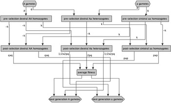
I will not discuss at any depth either what it means to causally interpret equations or how such interpretations are linked to directed acyclic graphs, although I will consider an example of applied population genetics in section 3 for which I draw a graph (fig. 1). The reader unfamiliar with causal graphs and causal equations need simply interpret the arrows in the graph as causal relations and know that causally interpretable equations have the causes on the right of the equal sign and the effects on the left. For an introduction to directed acyclic causal graphs and the causal interpretation of equations, see, for example, Glymour, Scheines, and Spirtes (Reference Glymour and Cooper1993), Pearl (Reference Morreau2000), or Woodward (Reference Walsh, Lewens and Ariew2003).

My main contribution comes in the next section, in which I state the proviso that can be appended to causal equations in classical population genetics to give them definite testable implications. In order to have a definite context in which to discuss my proviso, I consider an application of population genetics on the part of Michio Hori (Reference Hedrick1993), who causally explains the dynamics of a cichlid fish population by applying a population genetics model of frequency-dependent selection to it. I then provide a robust defense of my proviso and consider some objections to it. Section 8 modifies the proviso in the face of a technical challenge.

I have no evidence that the replacement for the phrase ceteris paribus that I suggest for classical population genetics will rescue causal equations in other special sciences from the dilemma presented by the alternatives of falsity and vacuity. However, my proviso is generated on the basis of a couple of conceptual maneuvers, “tricks,” which should be usable elsewhere too. In the conclusion, I discuss how my approach might be generalized.

2 An Alternative to Ceteris Paribus for Classical Population Genetics

I have based the proviso I developed for causal equations in classical population genetics on the one offered for applications of fundamental physics by John Earman, John Roberts, and Sheldon Smith (ERS). They offer their proviso in response to a putative example of a law of fundamental physics that is supposed to hold only ceteris paribus, specifically Marc Lange's “law” that a metal bar will expand when heated. Lange claims that this generalization holds only provided the bar is not being hammered on, is not encased in rigid material, and is not subject to indefinitely many other defeating influences. Earman, Roberts, and Smith write, “This list [of defeating influences] is indefinite only if expressed in a language that purposely avoids terminology from physics. If one helps oneself to technical terms from physics, the condition is easily stated: The ‘law’ of thermal expansion is rigorously true if there are no external boundary stresses on the bar throughout the process. Other putative examples of indefinite conditions can likewise be easily stated within the language of physics” (Reference Earman and Roberts2002, 284). External boundary stresses are forces applied to the surface of the bar; hammers, rigid materials, and anything else that would keep a metal bar from expanding when heated will count as an external boundary stress. ERS's talk of external boundary stresses groups together all potential defeaters and bans them in one fell swoop. The proviso is remarkable for a couple of other reasons, too.

First, notice that ERS's proviso is not something one can know automatically or without any possibility of error. Rather, they have provided a proviso that is meaningful because we can regard it as holding for some bar that is being heated, without first checking that the bar is expanding. My proviso, just like that of ERS, is not something one can know automatically or in some error-proof fashion, and it is equally the sort of thing one could know holds for some system without first determining whether a system of causal equations to which the proviso is attached accurately captures the dynamics of the target system. Second, note that ERS self-consciously use the language of physics to state rigorously the conditions under which physical laws hold; I will use the language of causation to state rigorously the conditions under which causal claims in classical population genetics hold.

A preliminary version of my proposal for a proviso to replace the vacuous phrase ceteris paribus that is usually attached to causal laws of the sort deployed in classical population genetics to save them from falsity is as follows:

To understand proviso 1, we need an explicit understanding of the following items: (1) what makes a cause pervasive, (2) what makes a cause interactive, (3) what nonpervasive causes are idealized away in classical population genetics, and finally, (4) how different values for causal variables are distinguished. I tackle these clarifications in turn.

A cause is pervasive if it affects all population members, rather than just some of them, at any given lifecycle stage. In the case of population genetics, a pervasive cause operating at one stage of the lifecycle will affect all the contemporaneous individuals at that lifecycle stage. Whether a cause is pervasive is a matter of how it is modeled. A pervasive cause may affect all population members by inducing changes in their probabilities of reproduction, rather than fully determining the reproductive output of the individuals subjected to it, and nonetheless count as pervasive; the causal influences modeled by Hori are like this. Whether some causal influence counts as pervasive in classical population genetics is a matter of whether the population is explicitly subdivided into distinct groupings in the mathematical model such that only some population members are subject to its influence, as in variable selection models (Hedrick Reference Glymour, Scheines and Spirtes2005, 210).

One cause is an interacting factor for another cause if the latter cause has a different influence on some effect depending on the value taken by the interacting factor. Cartwright (Reference Cartwright1979) offers a gripping, if somewhat imaginative, example of an interacting cause. Imagine I drink an acid poison. Normally, this will kill me since drinking an acid poison causes death. However, if I have just drunk an alkali poison, drinking an acid poison will save my life. This means that the recent consumption of an alkali poison is an interacting causal factor for acid poison intake when acid poison consumption is considered as a cause of death. In the context of no recent consumption of an alkali poison, drinking acid kills, while in the context of recent alkali poison consumption, drinking acid saves lives. The influence of any sort of cause can exhibit this sort of dependence on the value taken on by an interacting causal factor.

In classical population genetics, some nonpervasive causes are explicitly idealized away so that deterministic models can be deployed rather than stochastic ones. Once again, Hori's model is like this. The causes that are idealized away are informally referred to as those that produce drift; they result in “random changes in allele frequency” (Gale Reference Fodor1990, 13; Gillespie Reference Gildenhuys1998, 19; Hedrick Reference Glymour, Scheines and Spirtes2005, 304). Such causes have the same impact on all population members, regardless of what type they are, and exhibit no statistical associations with rival types (Gildenhuys Reference Gale2009). We can often idealize these causes away because they do not tend to swing relative frequencies in any particular direction over the long term. However, other causal influences that beset only some population members cannot be idealized away or left out of classical population genetics equations. For instance, statistical associations or interactions between target alleles and causally active alleles nearby on the genome must be officially recognized in classical population genetics through the use of multilocus selection models suitable for populations in linkage disequilibrium, while variable selection models are necessary for gene-by-environment interactions (Christiansen Reference Cartwright1975; Hedrick Reference Glymour, Scheines and Spirtes2005, 213).

Finally, to deploy proviso 1, it must be possible to assign values to causal variables, specifically to interacting factors, in a nonarbitrary fashion, a matter that is especially pressing in the case of continuous variables. If temperature is an interacting factor for some system of causal equations, we cannot limit the deployment of the equations to circumstances in which the ambient temperature is identical to the temperature at which the evidence for the equations was collected, at least not when temperature is measured in tiny fractions of degrees Celsius. The natural way to carve variables into values is to require that causal variables take on different values whenever the causes have a different impact on any of the effects in question, the y_n. So, interacting factors take on values that are different from those they took on when the evidence for f_n was collected, in any circumstance in which their impact on the value taken by any of the y_n is different. In many cases, small variations in temperature, for example, will not count as different values for temperature when it is conceived as a causal variable because temperature will not have a different influence on many effects when it changes only slightly. Again, Hori's fish are like this. Although great changes in the temperature of the lake that the fish inhabit would certainly scupper the equations Hori proposes for calculating the dynamics of cichlids, small variations in temperature would have no impact on the cichlids’ dynamics. Understanding how to tell when an interacting causal factor has taken on a different value requires knowing something about how it functions as a causal influence on the effect of interest. But knowing whether some interacting cause has taken on a different value does not require first checking whether the f_n hold, so this requirement brings no threat of circularity or vacuity.

It should now be possible to see that when completed with the above proviso, the claim that x causes y does have definite and meaningful implications. It means that the values of y ₁ through y_n can be inferred from the values of x ₁ through x_n for some system over which the equations are applied, provided the proviso holds. It also means that we can change the value of some y if we intervene on a system and change the value of some x, again provided the proviso holds. Finally, it means that the f_n explain the y_n, provided the proviso holds. The proviso has a definite content, too. The conditions in which we use causal equations to infer system dynamics must be like the conditions in which the evidence for the equations was collected, and the conditions in which the evidence was collected are a definite set of conditions. Furthermore, the conditions must be the same in a specific and definite way: all the pervasive causes of the y_n that are not represented in our causal equations (and are not causes or causal effects of those that are represented and are interacting factors for them in their influence on the effect variable) must take the same values in the conditions in which we use the equations to infer system dynamics as they took when the evidence used to affirm the equations was collected; additionally, all the nonpervasive causes of y must be included among the x ₁ through x_n, be their causal effects, or be explicitly idealized away.

Note how, when coupled with proviso 1, population genetics equations do not hold over a range of conditions in which those conditions vary in causally relevant ways. Of course, some conditions will be irrelevant to the dynamics of populations, and these can be allowed to vary in any way imaginable: most natural populations do not undergo different dynamics, depending on whether it is Monday or Tuesday. But proviso 1 is worded so that there is exactly one set of causally relevant conditions in which any population genetics equation functions as a tool of inference for a given system. Those conditions are ones in which pervasive interacting causal factors that are not represented in the equations (and are not causes or causal effects of ones that are) take on exactly the same values as they did when evidence for the equations was collected, and unrepresented nonpervasive causal influences that are not idealized away do not vary among population members.

This may strike the reader as far too strong a condition. Surely there is a range of conditions in which causal equations hold, a range in which causal connections are robust or invariant. In one sense there is. As discussed above, Hori's equations will capture the dynamics of his fish population, even when the lake temperature is slightly different from what it was when Hori collected his evidence. However, in such cases, I propose to understand lake temperature as taking the same value, when considered as a causal variable, despite taking two different values, when measured in degrees Celsius. Temperature takes on the same value as a causal variable, despite taking on different values in degrees Celsius whenever its impact on the dynamics of Hori's cichlids is the same as it was when Hori collected his evidence. So instead of trying to pick out a range of conditions in which causal equations function as tools of inference, I require that we carve pervasive interacting causal variables into values such that those variables only take on values that are different from the ones they took on when evidence was collected when they have a different impact on system dynamics. This allows me to state a proviso that picks out a definite set of conditions, rather than a range of conditions, that must be in place for some causal equations to be deployed.

Compare how, in Earman and Roberts’ discussion of Hempel's account of the provisos required for applications of fundamental physics, physical theory implies the same sort of conditional as that implied by classical population genetics: “What we can hope to derive from [theory] T are consequences of the form P→S, where again S is a logically contingent sentence whose nonlogical vocabulary belongs entirely to V_A [antecedently understood vocabulary] and P is a ‘proviso’ that requires the use of V_C [theoretical vocabulary]” (Reference Darden and Cain1999, 442). For applications of causal equations and applications of fundamental physical ones, what the provisos provide is a qualification that must be fulfilled for implications to be drawn from the equations for the observable systems.

3 An Example from Applied Population Genetics

The reader may well remain skeptical that the proviso I suggest does what it is supposed to do, and I will argue for it in a moment, but to make the case for proviso 1 it will be helpful to have at hand an example of an application of classical population genetics. Hori (Reference Hedrick1993) claims of a population of cichlid fish in the African Rift valley that a polymorphism that results from a single genetic variation is maintained in that population by frequency-dependent selection. Perissodus microlepis approaches prey from behind to snatch several scales. The mouths of these predators are angled either to the left or the right, making some left-handed (dextral) and others right-handed (sinistral). The fish only ever snatch scales from one flank of their prey, with right-handed fish favoring the left flank and left-handed fish favoring the right flank. The allele that produces dextrality is dominant, so that any cichlid with at least one dextral allele is dextral.

The cichlids have relatively poor hunting success, succeeding in snatching scales only about one-fifth of the time they attempt to do so, and this is because their prey are aware of them and guard against their assaults. The more frequent predator morph, whether dextral or sinistral, is at a disadvantage because the prey guard their left or right flank more vigilantly when that flank is the subject of a greater number of assaults. Each morph decreases the hunting success of like morphs and increases that of rival morphs by altering the flank-guarding behavior of the prey. Increased guarding by prey leads to fewer successful assaults by the more common predator. Accordingly, selection for rare types keeps both morphs at intermediate relative frequencies in the population.

In order to underwrite his claim that the selection regime among the cichlids will lead to a sustained polymorphism, Hori references a discussion of evolutionarily stable strategies in which a discrete generation model of frequency-dependent selection leading to a stable polymorphism is discussed (Cresswell and Sayre Reference Christiansen1991). Technically, the model considered in that article is suitable for haploids rather than diploids, and the cichlids are diploids. The model is adequate since diploid zygotes that exhibit complete dominance and random mating, as do Hori's cichlids, behave just as variant haploids do, at least in cases of frequency-dependent selection of the sort that Hori considers. Nonetheless, it would be better for our purposes here to consider a set of equations appropriate for selection in a diploid population. Accordingly, an idealized system of equations for frequency-dependent selection on diploid populations that is approximately appropriate for Hori's population is

where , , , p is the current-generation frequency of the A allele, p′ is the next-generation frequency of the A allele, q is the current-generation frequency of the a allele, q′ is the next-generation frequency of the a allele, and k is a coefficient expressing the extent to which zygotes affect the reproduction of their fellow population members.

For a population whose dynamics are governed by the above equation, we get a stable polymorphism at p = .25, which under random mating leads us to expect intermediate frequencies for both types of fish, the relative frequency around which the fish oscillate during Hori's study.Footnote ³ Hori clearly means to explain the persistence of the polymorphism as the result of frequency-dependent selection: “the handedness of this scale-eater is a documented example of a polymorphism maintained solely by frequency-dependent selection through prey-predator interaction” (Reference Hedrick1993, 218). But equation (1) can only be used to infer the dynamics of the handedness alleles, provided that proviso 1 holds for the population.

It is worth making clear how, for Hori, a grip on the causal influences of the handedness alleles is critical to his explanation of the dynamics of the two morphs. Hori runs a number of statistical tests to justify the causal scenario he envisions as what explains the dynamics of his fish population. Scales from the left and the right flanks of the cichlids’ prey appear different under a microscope. The claim that being left-handed causes the cichlid to attack the right flank of prey fish while being right-handed causes the cichlid to attack the left flank implies a covariance between fish morphologies and the appearance of the scales in the cichlids’ stomachs. Hori confirms this covariance observationally. Hori also conducts an experiment, using the prey fish as lures on fishing lines, to show that the cichlids only ever attack one flank of their prey. Similarly, that a single genetic variation causes differences in handedness would imply Mendelian statistical relationships between the morphologies of broods and the morphologies of the adults guarding them, something that Hori also confirms observationally. Hori is further able to track the oscillation in frequency of the two morphs through their lifecycle by sampling the fish population and thereby establishes that smaller, younger juveniles typically show the opposite bias in relative frequency to that seen among larger, older adults, providing evidence that the rare types have more reproductive success. Hori conducts more tests than this, but in one way or another, all of Hori's statistical tests serve to justify the causal scenario he attributes to his population. Hori traces out the implications of the causal scenario he envisions as what explains the cichlids’ dynamics and then verifies that those implications do in fact hold in the natural population.

Using the now widespread formal apparatus of directed acyclic graphs, we can exhibit the causal relationships that justify the deployment of equation (1) above for an idealized (deterministic, discrete generation) version of Hori's fish population. The relationship between causal facts and mathematical models is left implicit by Hori; population geneticists generally leave this connection implicit. Directed acyclic graphs serve as a formal tool to express the inferential connection between causal facts and mathematical models. Figure 1 is a graph for Hori's fish population.

Figure 1.

With the exception of the average-fitness node, all the nodes in the graph represent frequencies (or equivalently absolute numbers) of gametes or zygotes.Footnote ⁴ The coefficients between the first and the second array of nodes, p and q, express the Hardy-Weinberg law for randomly mating populations, that is, the rates at which gametes (sperm and eggs) bearing the variant alleles combine to form zygotes (fish). The second set of coefficients measures the extent of the causal influence that rival zygotes have on one another's viability during maturation. Note how each type of zygote benefits individuals of the opposite type and is harmful to individuals of the same type, something that is reflected in the sign on the k coefficient. The third set of coefficients expresses the contributions of the zygotes to the gametes of the next generation, as well as the contributions of the zygotes to the average fitness of the population, both of which are proportional to the zygotes’ frequencies. Among the heterozygotes, meiosis is represented as a coefficient on the final set of edges, too (hence, the coefficient on some of the edges rooted at the heterozygotes is a product, 1/2 × 2pq). We can derive equation (1) from this graph, if (with the exception of the influence of the average-fitness node) we treat all the functional relationships between ancestor nodes and descendant nodes as additive and form products from the coefficients on the edges and the values of the nodes at the feet of the edges. The average fitness functions as a divisor.

4 Arguing for Proviso 1

Having established that Hori's research provides us with an example of a causal equation from classical population genetics that is used as a tool of inference to explain the dynamics of a real population, I now turn to argue that proviso 1 can function to restrict the application of the system of equations that is approximately appropriate for Hori's fish to those circumstances in which it can be used to make inferences about their dynamics. It is at least imaginable that things will change among the cichlids such that equation (1) can no longer be used to make inferences about the dynamics of the handedness alleles. If we want to use equation (1) to predict that the population will remain polymorphic, or explain that it does so, we will have to know that things have not changed in a way that will undermine equation (1).

I claim that knowing that proviso 1 holds is exactly what we need to know to continue to deploy equation (1) over Hori's cichlids. By extension, the proviso is supposed to apply to population genetics equations in general. My claim is essentially that were things to change with respect to the cichlids in a way that would scupper the use of equation (1) to explain the dynamics of Hori's cichlids, the proviso would expressly forbid deployment of it. Furthermore, it would do so in a noncircular fashion, without forbidding the deployment of equation (1) on the grounds that it failed.

It is fairly easy to think up situations in which proviso 1 might fail to hold for Hori's cichlids in the future. For instance, were there to arise in the population a statistical association between one of the handedness alleles and a novel beneficial genetic variation at a nearby locus, then equation (1) would fail as a tool of inference for population dynamics. But such a beneficial allele at a nearby locus would constitute a nonpervasive causal influence not accounted for in equation (1), and so the proviso would bar us from applying equation (1) in such a scenario. Equation (1) might also fail if the sinistral but not the dextral fish become prized by fishermen. However, the fishermen constitute an interactive causal influence on the system's dynamics, having a different impact on the success of different types of fish or, equivalently, altering the causal impact of handedness on viability. The proviso instructs us not to apply equation (1), should such fishermen have the sort of impact that is being imagined, because the fishermen, considered as a causal influence, are taking on a different value than they took on when the evidence for equation (1) was collected.

That last claim might strike the reader as odd because it is natural to think of the fisherman as a causal influence that was not operative at all when Hori did his research. In fact, one of the tricks behind my proposal is to think of many defeating causal influences as operative even when they have no impact on system dynamics. Although it is counterintuitive to do so, the way to think of the fishermen is as an interactive causal influence that actually was at work when the evidence was being collected. It is just that the fishermen were a causal influence that took a null value, such that they had no influence on population dynamics. Many causal variables are like this, having an influence when they take one value but having no impact when they take another value.

A variable takes on a null value whenever dropping it from an equation entirely would have no impact on the mathematical calculation performed (we will consider an example in a moment). It is legitimate to drop variables from equations when they take null values, and it is equally legitimate not to insert into an equation variables that represent causal influences with null impacts, when one is formulating the equations in the first place. But causes may go unrecognized in causal equations, neither because they are not causes of the effect nor because they are not at work; instead, they may go unrecognized because they take null values.

To see how this works, let us represent the impact of the fishermen with a fondness for sinistral fish formally, by adding some definite coefficients to equation (1) so as to introduce the fishermen into the model. Let us say that the fishermen variable takes on two values, 1 and 0.8, corresponding to absence and presence. Using g for fishermen, equation (1) with the fishermen explicitly recognized is as follows:

When Hori collected his evidence, g was set at 1, a null value, in accordance with the absence of the fishermen. If the population were to be confronted by fishermen with a preference for sinistral fish, g would take the value 0.8.

It is not the case, however, that we must represent the influence of the fishermen formally, as in equation (2) above, in order to make inferences about the dynamics of the cichlid population. But if we do not mention the fishermen in our equation and use equation (1) instead of (2), then we must take it that the value taken on by this interactive causal influence remains the same as the one it took on when Hori collected his evidence. Equation (2) just reduces to (1) when the fishermen are absent and g = 1, the conditions in which Hori collected his evidence. So, the evidence justifies using equation (1) to infer the dynamics of the system only insofar as the fishermen continue to be absent, that is, continue to have a null impact on the dynamics of the system.

While there are indefinitely many pervasive interactive causal influences on the cichlids, we can calculate the cichlids’ dynamics using the relatively simple equation (1) because the bulk of these causal influences have null impacts. Indeed, there are only “indefinitely many” conditions necessary for equation (1) to hold if we try to count them without using causal language. But if we group defeaters using causal language, then we can say with a definite proviso what all the pervasive interactive causal factors must be like for us to use some equations as inferential tools. They are causes that must not change their values, provided they are not represented in the equations used to infer the dynamics of the population and are not causes or causal effects of those that are. Compare this to how ERS gather together all the defeating factors for Lange's law under the rubric of “external stresses.”

Nonpervasive causal influences that are not mentioned in equation (1) are also easy to pick out using causal language since we can contrast the individuals in the system beset by them to those individuals that are not beset by them. The second sentence of proviso 1 essentially rules out any of our population members varying with respect to the nonpervasive causal influences to which they are subject, unless these are explicitly represented in the equations used to infer the dynamics of the system or are explicitly idealized away. That condition, too, may seem too strong because surely individual fish are subject to different causal influences that affect their viability and reproduction. But recall that by invoking deterministic population genetics equations, Hori idealizes away the causes that are responsible for drift. These are nonpervasive causal influences on the reproduction of the fish that are noninteractive (they have the same influence on the dextral and sinistral fish) and are not statistically associated with either morph. The cichlids can vary in their exposure to these without undermining equation (1) because such causal influences have no sustained directional or stabilizing influence on the dynamics of the population (Gildenhuys Reference Gale2009).

I should note, though, that it is not possible to explicitly recognize the appearance of a beneficial mutant allele near to the handedness locus by transforming equation (1), as we did when we used equation (2) to recognize the impact of the fishermen. Instead, the occurrence of such a statistical association would require us to ditch equation (1) in favor of a multilocus selection model. Models of this sort can be used to recognize interactions between alleles at different loci or statistical associations between alleles nearby on the genome. As it turns out, causal influences are recognized in the formalism of classical population genetics, both through the deployment of parameters that quantify their impact as well as through the use of distinct systems of equations that are appropriate for causally distinct sorts of systems.

Note how the situation here parallels the case of fundamental physics. Just as it is impossible to rule out all the defeating conditions for the law of thermal expansion without using the language of physical theory, it is impossible to list all defeating conditions for Hori's causal claim about the cichlids without using the language of causation. But we can take care of all the exceptional cases (selective fishermen, genetic mutations, bizarre alien fish eaters, and anything you care to imagine) using a finitely expressible proviso if we use cause-talk to formulate it.

Indeed, the very fact that philosophers have no difficulty thinking up defeaters for causal equations is evidence that they have an intuitive grip on what features a defeater must have in order to undermine a putative causal relationship. My suggestion is that this intuitive knowledge amounts to the understanding that positing changes in the values of interacting causal factors is sufficient to undermine a causal relationship. (In the case of population genetics, positing novel causal influences that affect only some members of the population can undermine the use of population genetics models to make inferences about system dynamics, too.) But that anyone can come up with a great many defeaters for any causal claim should actually induce us to believe that there must be a general way of grouping these together as instances of one or a few sorts of things. It is an implicit understanding of what features a defeater must have, what sorts of things they are, that makes it possible for us to think up instances of them ad nauseam.

5 Objection: The Proviso Is Versed in Cause-Talk

I now turn to consider some objections to proviso 1. First, proviso 1 is versed in causal language, so one must have a grip on how to ascertain causal relationships in order to deploy the proviso. However, “cause” has not been defined in a noncircular fashion, and it is notoriously difficult to state the circumstances in which causal relationships may be affirmed. An objector might refuse to countenance proviso 1 until she is presented with an account of how causal relationships are ascertained.

It is certainly true that one major problem with causation concerns how one might put oneself in a position to affirm causal relationships. However, the problem is not utterly intractable. Much recent work on causal inference has been oriented toward providing sufficient grounds for affirming causal relationships on the basis of statistical data along with some plausible assumptions (see, e.g., Glymour et al. Reference Glymour and Cooper1993; Glymour and Cooper Reference Gillespie1999; Pearl Reference Morreau2000; Hulten, Chickering, and Heckerman Reference Hori2003; Zhang and Spirtes Reference Woodward2008). Statistical data, combined with principles of inference such as the causal Markov condition, minimality, and faithfulness, are sometimes good enough to zero in on a specific causal structure for some system, when only that causal structure would imply the statistical data. Earlier, we saw that Hori was informally engaged in a similar kind of evidence-based reasoning. He infers from the fact that a great many implications of a causal relationship hold in some system to the fact that the causal relationship itself does.

Reasoning on the basis of evidence in this way is not error proof or logically compelling. But it is surely too much to ask that causal relationships be affirmable on logically compelling grounds. Fundamental physical theories, for instance, cannot be established in such a fashion because they involve unobservables.

Of course, if a critic is unwilling to countenance causal inference in the first place, then she will regard proviso 1 as meaningless. But she will have a problem with claims of the form x causes y no matter what, whether they are coupled with my proviso, ceteris paribus, some other alternative, or nothing at all. My aim is not to convince a causal skeptic to lay her faith in the sort of evidential reasoning used to affirm causal relationships. My aim is to show how causal equations can be coupled with a definite proviso so as to give them definite implications for system dynamics; I simply assume that we can get a grip on causal facts using evidence.

6 Objection: The Proviso Is Not Helpful

The proviso I propose for causal laws makes explicit reference to the values taken on by causal variables at a specific time, when evidence for them is collected. That is part of what gives the proviso its definite meaning. But one might object to my proposal on the grounds that all causal influences over a system of interest that we recognize as such will be those that appear in the equations we deploy for the system. The proviso I have suggested commits us to facts about the values taken on by other causal influences, those that, by appearances anyhow, we did not explicitly recognize as potentially interacting factors when the research was done. Because we are not aware of causal influences not featured among the x ₁ through x_n, since otherwise we would have included them in our equation (the objector has us imagine), how does attaching proviso 1 to some system of equations help us to deploy those equations to reason about natural systems?

First, note that my proviso is no different from that of ERS in this regard. While ERS's proviso commits them to facts about stresses acting on the bar that are not mentioned in Lange's generalization, my proviso commits me to facts about causes not represented in causal equations. So the objector is effectively aiming to undermine not only the sort of provisos we need for causal equations but the sort we need to apply any dynamical theory, something that should make us dubious.

Indeed, the objection is based on a misunderstanding of what it means for causes or forces to be left out of an equation. While the absence of variables representing either forces or causes in an equation makes it appear as though they were overlooked, what is really going on is that the evidence used to deploy the equation justifies leaving the forces or causes out of the picture. Causes or forces may go unmentioned in a system of equations, but the evidence would not have warranted their disregard had they taken non-null values. This is true, anyway, in cases in which our evidential reasoning does not let us down, something we can never fully guarantee. But whenever we use evidence to affirm a causal relationship, we must assume the evidence is not conspiring against us. One way in which that assumption manifests itself is in researchers’ commitment that no latent variables with an impact on system dynamics have been overlooked.Footnote ⁵ That assumption does not amount to the assumption that there are no causes of the effect that are not represented explicitly in the system of equations; instead, it amounts to the assumption that unrepresented causal influences take null values in the system. Evidence can license taking this attitude to unrepresented causes, even if those causes cannot be picked out in noncausal terms, even if they cannot be picked out as anything but other pervasive interactive causes of the effect.

In the cases at hand, if we really imagine collecting evidence to license the deployment of Lange's law for some real metal bar, it would be bizarre to suppose that we would overlook a man with a hammer pounding on the bar, or a rigid structure encasing it, and so on. Similarly, when Hori did his research, it is reasonable to suppose that his evidence would have turned up discerning fishermen and the like. What is critical, however, is the general point: evidence can license us not only to disregard the causal influence of the fishermen but also to disregard all other pervasive interactive causal influences on Hori's fish, pervasive interactive causal influences that, unlike the fishermen, we pick out in no other terms except as such.

Evidence that a cause or a force has no impact on some system is not, of course, logically compelling, but when dealing with theories that require us to countenance causes or unobservables, we can do no better than to evaluate what causes or forces have an impact on system dynamics using evidence. When the evidence indicates that a cause or a force has no impact on system dynamics, it is left out of the equation we apply to the system, and that in turn means the equation only applies when the left-out forces and causes continue to have no impact: hence, the provisos.

7 Objection: How Are We Supposed to Know What Causes Are Covered by Proviso 1?

The readers who remain dissatisfied with proviso 1 may find themselves wondering how we are supposed to know what the causal influences covered by proviso 1 are. This sort of concern can be understood in two different ways. On the one hand, it might be understood as an appeal for more specificity: “Tell me how to pick out these potentially ‘defeating’ causal influences to which proviso 1 refers.” On the other hand, the concern could be understood as epistemic in nature: “How are we supposed to figure out that the pervasive causal influences picked out in proviso 1 take the same values as they did when the evidence was collected, and how are we supposed to figure out that no new nonpervasive causes have appeared since the collection of evidence?” I will deal with these concerns in turn.

With respect to the appeal for further specificity, I can only respond that proviso 1 is versed in causal language on purpose. Indeed, one of the insights behind the proviso is supposed to be that causal language is appropriate for a proviso for causal equations, just as the language of physical theory is appropriate for a proviso for equations drawn from physical theory. The proviso picks out potential defeaters using causal language because any alternative vocabulary will inevitably be either too specific or too general or both. For instance, we cannot trade in proviso 1 for a proviso that requires that the “environment” be the same in the context of application as it was in the context of investigation, for some specific system of causal equations such as equation (1). This is in part because some environmental features will be irrelevant to the dynamics of the genetic variations among the cichlids, making such a proviso unnecessarily strong, perhaps even impossibly so. It is also because some things that are relevant to the dynamics of genetic variations are not environmental in origin; they are genes at other loci, sex differences, other population members, genomic imprints, or what have you.

The feature that everything covered by the proviso must share is causal relevance to the dynamics of the population, indeed causal relevance of a specific sort. There is no alternative characterization that will do the trick, at least none that I or anyone else has been able to think up. But we do not need an alternative characterization of “defeaters” to assert a meaningful proviso. A causal characterization is still a characterization. We need not be able to pick out potential defeaters in any terms other than those used in proviso 1 for that proviso to be meaningful. If one regards cause-talk as meaningful, and one must do this to be in the business of evaluating a proposed proviso for causal equations, then the causal characterization of potential defeaters used in proviso 1 must be regarded as meaningful.

With respect to the epistemic concern about how the causes discussed in proviso 1 are to be picked out, it should be acknowledged that there is no reason to think that we will generally be able to put ourselves in a position to affirm proviso 1 when applying classical population genetics. But while it may seem that affirming proviso 1 is very difficult to do, that is really beside the point. I am trying to say explicitly to what you need to commit in order to deploy some causal equations as tools of inference. I am aiming for a nonvacuous proviso for causal equations, not one that is necessarily easy to check. Indeed, our physical theories can be difficult to apply for epistemic reasons, too: the dynamics of a falling leaf cannot be predicted using physical theory because we cannot expect to know how, when, and to what extent the leaf will be subject to the forces that affect its dynamics as it falls. But that is no reason to question provisos of the sort proffered by ERS, and similar epistemic difficulties are no reason to question proviso 1.

That said, it is not in fact uncommon to have very good reasons for taking it that causal influences will at later times take on the same values as they did earlier on, even when one does not know what those causal influences are or even whether they exist at all. I do not endorse Nancy Cartwright's broader views on natural laws, but one of her better insights about causality concerns the role of shielding in setting up situations in which we can safely develop expectations on the basis of causal relationships (Reference Cartwright1999, 29, 67). A laboratory is very good shield; in a lab, just about everything that even could be an interacting factor for a cause takes on the same value from one day to the next, unless it is expressly altered by an experimenter. A causal relationship affirmed on the basis of evidence collected in a lab can license very strong expectations about what will happen to the system in the laboratory in the future because the laboratory provides a shield to all sorts of changes in conditions, whether or not those conditions are interacting factors for the causal relationship of interest.

In laboratories, we can shield systems very effectively. Simpler examples of shields include the casings around batteries and computer parts. But even in the absence of shielding, it might not be unreasonable to develop expectations about the values taken on by interactive causal influences. A couple of degrees Celsius difference in the temperature of the lake water will not matter to the dynamics of Hori's fish, and the lake will not freeze or begin to boil anytime soon. We also have a decent grip on the rates at which alleles mutate, and we know that beneficial mutations are especially rare. Indeed, we can take the same sort of attitude we do to our exemplary defeaters of Hori's equations, the lake temperature and the beneficial mutations, to every causal influence that could defeat Hori's equations. We can do so by conceptualizing the potential defeaters in causal terms, and we can do this even though we lack any alternative way to conceptualize these causal influences. Indeed, I claim that were one to deploy Hori's equations to develop expectations about the dynamics of the Perissodus microlepis over the next year, one would implicitly do just that.

8 A Technicality

The reader may have already noticed a flaw in the above proviso. Consider a scenario in which evidence is collected for some system that yields this causally interpretable equation:

where all the variables take on value 1 or −1. Let us imagine the research we used to affirm equation (3) involved 10 trials. As it turns out, there are unmeasured causal influences x ₃ and x ₄ that interact with x ₁ and x ₂, and, in the tenth trial, both x ₃ and x ₄ took on different values for all the individuals in the system on which data were collected. Putting this in formal terms, let us imagine that what is really going on is this:

where, just like x ₁ and x ₂, both x ₃ and x ₄ may take on value 1 or −1. In the first nine trials, x ₃ and x ₄ both took value 1, while in the tenth trial they were both equal to −1, so that in each trial they had the same impact on the system together. Even though x ₃ and x ₄ varied when the evidence was collected, because they happened to vary such that they cancelled each other out, the evidence still licensed the researcher to characterize the system using equation (3), which makes no mention of x ₃ and x ₄. However, because x ₃ and x ₄ took on different values at different times when the evidence was collected, the proviso as it is stated does not make sense for equation (3): there is no fact of the matter about the value taken on when the research was done by pervasive interacting causes not included on the right-hand side of equation (3) because some pervasive unmeasured interacting causes, x ₃ and x ₄, did not take on invariant values. (Because they affected all population members in each trial, x ₃ and x ₄ still count as pervasive causal influences; they are just variant pervasive causal influences.)

Accordingly, the proviso I put forward above has to be modified a little. I make a conservative amendment. While invariant pervasive interactive causal influences that are not featured among the causes in some system of equations, and that are not effects of these, must not take new values when the equations are deployed, sets of variant pervasive interactive causes must take on one of the sets of values they took on when the evidence was collected. Here is the new proviso 1:

In our little example, the proviso requires that x ₃ and x ₄ must both take on value 1 or both take on value −1 in any context in which one uses the causal claim (eq. [3]) to make inferences about what will happen in the system because the variant causes x ₃ and x ₄ together took on one of those two sets of values when the evidence for equation (3) was collected.

My solution is a conservative solution to the technical difficulty with which we began, for it is imaginable that some sets of unmeasured interactive causal influences could take on sets of values that render them innocuous, even though they never took on those sets of values when the evidence was collected. So, we can imagine that x ₃ could take on one of three values (1, 1/2, and −1), while x ₄ could take on 1, 2, and −1, and although they together did not take on values 1/2 and 2 at the same time when the evidence for equation (3) was collected, should they together do so in the future, we could deploy equation (3) to make inferences about what would happen to the system in such circumstances.

However, we do not want to undertake the kind of commitment that ERS have criticized as vacuous; we do not want to say that “x ₁ and x ₂ cause y except when they do not.” When we say of sets of interactive causal influences that they must take one of the sets of values they took on when the evidence for some causal equations was collected, we are saying something definite about them. We are availing ourselves of the fact that the circumstances in which evidence was collected are a definite set of circumstances. But I cannot think of a noncircular way to pick out sets of values for unmeasured varying interactive causal influences that render them innocuous without making reference to the values they take when evidence is collected, so I cannot think of a proviso that would allow us to deploy equation (3) when x ₃ and x ₄ take the values 1/2 and 2, respectively. We cannot very well say that x causes y except when other variant causes of y are not innocuous.

My conservative solution to the flaw in the proviso will sometimes allow us to deploy causal relationships in fewer circumstances than we could in fact deploy them to make good inferences, but that is a minor sort of flaw. More important, my conservative solution does not license the deployment of causal laws in circumstances in which they will invite us to make bad inferences that do not preserve truth. Equally crucial is that my amended proviso has a definite meaning.

Finally, it is worth noting that it will probably be rare that pervasive interactive causal influences not represented in our equations vary but just happen to vary in a fashion such that they cancel each other out. I modified proviso 1 to cover cases involving covarying mutually canceling unrepresented pervasive interactive causal influences in order to make sure that the proviso says something definite about such cases so that it is not nonsensical. I was not motivated to modify proviso 1 so as to make it possible to exploit causal equations as often as possible. Indeed, covarying mutually canceling pervasive interactive causal influences may often cease to covary at later times. When we use causal equations secured by evidence from situations in which mutually canceling unrepresented variant pervasive interactive causes merely happened to covary such that they together had a null impact, we will often go wrong when we deploy the equations later on. We will have been unfortunate in our data collection. Using statistical data to hit upon definite lawlike relationships, causal or otherwise, is generally quite hard, and the possibility of incidentally covarying unrepresented mutually canceling variant pervasive interactive causal influences in the system from which we gather evidence is just one more hazard for such reasoning.

9 Conclusion

My aim in this article has been to offer an account of how the causal equations of classical population genetics can be supplied with provisos that are nonvacuous, such that the equations can function as strict laws or at any rate as meaningful tools of inference about the dynamics of the systems to which they are applied. My proposal relies on a couple of tricks that make it possible to state a nonvacuous proviso for classical population genetics equations. The first trick is to pin the applicability of causal equations to the conditions in which the evidence for them was collected. After all, when we generate causal equations for some system, we are at least willing to affirm that they capture the dynamics of the system when it was investigated. Because the circumstances of investigation occurred at a definite place and at a definite time, talk of such circumstances has a definite meaning. The second trick is to think of those circumstances as ones in which many causal influences that could defeat the causal equations were actually operative, although they took null values. These maneuvers are what makes it possible to talk about all the defeaters at once and to require that they do not change their values.

The two tricks just discussed should be usable for other systems of causal equations, those outside classical population genetics. For instance, consider how the development of preventative therapies for lung cancer would scupper the causal relationship between smoking and lung cancer. Evidence for the causal relationship between smoking and lung cancer was collected in a set of conditions in which preventative therapies were unavailable, conditions we should think of as those in which lung cancer prevention therapies functioned as causes but in which such causes were set to null values associated with their absence, such that they had no impact on lung cancer rates. So we should say that the causal claim “smoking causes lung cancer” is applicable to human populations only insofar as those populations resemble, in a specific way, the human populations that were used as evidence to ascertain the causal relationship between smoking and lung cancer. More specifically, the pervasive interactive causal influences on lung cancer in human populations over which we deploy the generalization “smoking causes lung cancer” must not take on values that differ from those such causes took in the populations from which evidence for that last causal claim was collected. This means, among other things, that everyone in the population must not make use of preventative therapies for lung cancer if we are to assert a causal connection between smoking and lung cancer within it.

Thus, the part of proviso 1 dealing with pervasive interactive causes should be appropriate quite generally for causal equations, at least for systems of causal equations that are deployed over populations of entities. However, simply out of caution, I am reluctant to affirm that all causal equations from all disciplines in the special sciences should be paired with proviso 1. I am uncertain whether the treatment of nonpervasive causal influences in classical population genetics matches the treatment of such causes in other special sciences. My general understanding of causal modeling in classical population genetics was critical to my development of proviso 1 for systems of equations in classical population genetics, and I simply do not know very much about causal modeling in other disciplines.

So, I claim to have gone some distance to specifying what sort of proviso is appropriate for causal claims in general. My two tricks—requiring that the conditions of application of causal equations resemble, in a definite way, the conditions of investigation and taking it that pervasive defeaters are operative in the conditions of investigation while taking null values—should provide the means to state provisos appropriate for other systems of causal equations. Furthermore, I expect that the first part of proviso 1, dealing with pervasive interactive causal influences, should have general applicability for causal equations concerning populations of entities in the special sciences.