2.1 Constitutive equations

We assume the fluids to be of generalized Newtonian type, in particular obeying the Herschel–Bulkley model, which includes Newtonian, power law and Bingham models. The dimensionless constitutive laws for Herschel–Bulkley fluids are

(2.6) $$\begin{eqnarray}\displaystyle & \displaystyle \dot{\unicode[STIX]{x1D6FE}}(\boldsymbol{u})=0\quad \text{if}~\unicode[STIX]{x1D70F}_{k}(\boldsymbol{u})\leqslant B_{k}, & \displaystyle\end{eqnarray}$$

(2.7) $$\begin{eqnarray}\displaystyle & \displaystyle \unicode[STIX]{x1D70F}_{k,ij}(\boldsymbol{u})=\left[\unicode[STIX]{x1D705}_{k}\dot{\unicode[STIX]{x1D6FE}}^{n_{k}-1}(\boldsymbol{u})+\frac{B_{k}}{\dot{\unicode[STIX]{x1D6FE}}(\boldsymbol{u})}\right]\dot{\unicode[STIX]{x1D6FE}}_{ij}(\boldsymbol{u})\quad \text{if}~\unicode[STIX]{x1D70F}_{k}(\boldsymbol{u})>B_{k}, & \displaystyle\end{eqnarray}$$

where the subscripts $k=H,L$ and the strain rate tensor has components

(2.8) $$\begin{eqnarray}\displaystyle \dot{\unicode[STIX]{x1D6FE}}_{ij}(\boldsymbol{u})=\frac{\unicode[STIX]{x2202}u_{i}}{\unicode[STIX]{x2202}x_{j}}+\frac{\unicode[STIX]{x2202}u_{j}}{\unicode[STIX]{x2202}x_{i}}, & & \displaystyle\end{eqnarray}$$

and the norms of these tensors (i.e. the second invariants), $\dot{\unicode[STIX]{x1D6FE}}(\boldsymbol{u})$ and $\unicode[STIX]{x1D70F}_{k}(\boldsymbol{u})$ , are defined by

(2.9a,b ) $$\begin{eqnarray}\displaystyle \dot{\unicode[STIX]{x1D6FE}}(\boldsymbol{u})=\left[\frac{1}{2}\mathop{\sum }_{i,j=1}^{2}[\dot{\unicode[STIX]{x1D6FE}}_{ij}(\boldsymbol{u})]^{2}\right]^{1/2},\quad \unicode[STIX]{x1D70F}_{k}(\boldsymbol{u})=\left[\frac{1}{2}\mathop{\sum }_{i,j=1}^{2}[\unicode[STIX]{x1D70F}_{k,ij}(\boldsymbol{u})]^{2}\right]^{1/2}. & & \displaystyle\end{eqnarray}$$

Since the parameters are dimensionless, we find $\unicode[STIX]{x1D705}_{H}=1-B_{H}$ and $\unicode[STIX]{x1D705}_{L}=m-B_{L}$ , with the viscosity ratio, $m$ , defined as

(2.10) $$\begin{eqnarray}\displaystyle m\equiv \frac{\hat{\unicode[STIX]{x1D707}}_{L}}{\hat{\unicode[STIX]{x1D707}}_{H}}=\frac{\hat{\unicode[STIX]{x1D705}}_{L}[\hat{V}_{0}/\hat{D}_{0}]^{n_{L}-1}+\hat{\unicode[STIX]{x1D70F}}_{L,Y}[\hat{V}_{0}/\hat{D}_{0}]^{-1}}{\hat{\unicode[STIX]{x1D705}}_{H}[\hat{V}_{0}/\hat{D}_{0}]^{n_{H}-1}+\hat{\unicode[STIX]{x1D70F}}_{H,Y}[\hat{V}_{0}/\hat{D}_{0}]^{-1}}, & & \displaystyle\end{eqnarray}$$

where $\hat{\unicode[STIX]{x1D707}}_{H}$ and $\hat{\unicode[STIX]{x1D707}}_{L}$ are viscosity scales for fluids $H$ and $L$ , respectively. For two Newtonian fluids, we recover $\hat{\unicode[STIX]{x1D707}}_{k}=\hat{\unicode[STIX]{x1D705}}_{k}$ . The Bingham numbers $B_{k}$ are also defined as

(2.11) $$\begin{eqnarray}\displaystyle B_{k}\equiv \frac{\hat{\unicode[STIX]{x1D70F}}_{k,Y}}{\hat{\unicode[STIX]{x1D705}}_{H}[\hat{V}_{0}/\hat{D}_{0}]^{n_{H}}+\hat{\unicode[STIX]{x1D70F}}_{H,Y}}. & & \displaystyle\end{eqnarray}$$

Note that based on the definitions of the Bingham numbers above, we always have $0\leqslant B_{H}<1$ and $0\leqslant B_{L}<m$ .

It is worth emphasizing that, in the above scalings, the ‘effective viscosity’ is used to produce the dimensionless groups, such as the Bingham numbers and the viscosity ratio, implying that we are dealing with the ‘effective’ versions of $B_{k}$ , $m$ , etc. This approach, which has been introduced in the recent literature (see e.g. Nirmalkar, Chhabra & Poole Reference Nirmalkar, Chhabra and Poole2013 and Thompson & Soares Reference Thompson and Soares2016), provides a reasonable framework to analyse the role played by viscosity in our displacement flows. Also note that our effective dimensionless groups can be easily converted to their more conventional forms using simple relations (Nirmalkar et al. Reference Nirmalkar, Chhabra and Poole2013; Thompson & Soares Reference Thompson and Soares2016).

3.1 Computing flux function

In this section we explain our method to find the stress and velocity solutions, from which the flux can be computed. For fixed parameters, including fixed $h$ and $\unicode[STIX]{x2202}h/\unicode[STIX]{x2202}X$ , equations (3.6) and (3.7) can be written as

(3.19) $$\begin{eqnarray}\displaystyle \frac{\unicode[STIX]{x2202}}{\unicode[STIX]{x2202}y}\unicode[STIX]{x1D70F}_{H,Xy} & = & \displaystyle \frac{\unicode[STIX]{x2202}P_{0}}{\unicode[STIX]{x2202}X},\quad y\in (0,h),\end{eqnarray}$$

(3.20) $$\begin{eqnarray}\displaystyle \frac{\unicode[STIX]{x2202}}{\unicode[STIX]{x2202}y}\unicode[STIX]{x1D70F}_{L,Xy} & = & \displaystyle \unicode[STIX]{x1D712}-h_{X}+\frac{\unicode[STIX]{x2202}P_{0}}{\unicode[STIX]{x2202}X},\quad y\in (h,1),\end{eqnarray}$$

showing that, in each pure fluid layer, the shear stresses are linear in $y$ .

For Newtonian displacements, the equations can be simply integrated to deliver the analytical solution for the flux function:

(3.21) $$\begin{eqnarray}\displaystyle q_{H}(h,h_{X},\unicode[STIX]{x1D712},m,\unicode[STIX]{x1D706}_{l},\unicode[STIX]{x1D706}_{u})=q_{H,A}(h,m,\unicode[STIX]{x1D706}_{l},\unicode[STIX]{x1D706}_{u})+q_{H,B}(h,m,\unicode[STIX]{x1D706}_{l},\unicode[STIX]{x1D706}_{u})(\unicode[STIX]{x1D712}-h_{X}), & & \displaystyle\end{eqnarray}$$

which includes an advective component ( $q_{H,A}$ ) and a buoyancy-driven component ( $q_{H,B}$ ), found as

(3.22) $$\begin{eqnarray}\displaystyle q_{H,A} & = & \displaystyle \frac{a_{11}\unicode[STIX]{x1D706}_{l}^{1}\unicode[STIX]{x1D706}_{u}^{1}+a_{10}\unicode[STIX]{x1D706}_{l}^{1}\unicode[STIX]{x1D706}_{u}^{0}+a_{01}\unicode[STIX]{x1D706}_{l}^{0}\unicode[STIX]{x1D706}_{u}^{1}+a_{00}\unicode[STIX]{x1D706}_{l}^{0}\unicode[STIX]{x1D706}_{u}^{0}}{c_{11}\unicode[STIX]{x1D706}_{l}^{1}\unicode[STIX]{x1D706}_{u}^{1}+c_{10}\unicode[STIX]{x1D706}_{l}^{1}\unicode[STIX]{x1D706}_{u}^{0}+c_{01}\unicode[STIX]{x1D706}_{l}^{0}\unicode[STIX]{x1D706}_{u}^{1}+c_{00}\unicode[STIX]{x1D706}_{l}^{0}\unicode[STIX]{x1D706}_{u}^{0}},\end{eqnarray}$$

(3.23) $$\begin{eqnarray}\displaystyle q_{H,B} & = & \displaystyle \frac{b_{11}\unicode[STIX]{x1D706}_{l}^{1}\unicode[STIX]{x1D706}_{u}^{1}+b_{10}\unicode[STIX]{x1D706}_{l}^{1}\unicode[STIX]{x1D706}_{u}^{0}+b_{01}\unicode[STIX]{x1D706}_{l}^{0}\unicode[STIX]{x1D706}_{u}^{1}+b_{00}\unicode[STIX]{x1D706}_{l}^{0}\unicode[STIX]{x1D706}_{u}^{0}}{c_{11}\unicode[STIX]{x1D706}_{l}^{1}\unicode[STIX]{x1D706}_{u}^{1}+c_{10}\unicode[STIX]{x1D706}_{l}^{1}\unicode[STIX]{x1D706}_{u}^{0}+c_{01}\unicode[STIX]{x1D706}_{l}^{0}\unicode[STIX]{x1D706}_{u}^{1}+c_{00}\unicode[STIX]{x1D706}_{l}^{0}\unicode[STIX]{x1D706}_{u}^{0}},\end{eqnarray}$$

where the coefficients $a_{ij}$ , $b_{ij}$ and $c_{ij}$ (with $i,j=0,1$ ) are functions of $h$ and $m$ only, and they are given in appendix A. If $\unicode[STIX]{x1D706}_{l}=\unicode[STIX]{x1D706}_{u}=0$ (i.e. no-slip at both walls), we retrieve

(3.24) $$\begin{eqnarray}\displaystyle q_{H}=\frac{a_{00}+b_{00}(\unicode[STIX]{x1D712}-h_{X})}{c_{00}}, & & \displaystyle\end{eqnarray}$$

which matches the flux function given in Taghavi et al. (Reference Taghavi, Seon, Martinez and Frigaard2009) for a displacement flow in a channel with no wall slip.

In a similar manner, the velocity profiles for Newtonian fluids can be also analytically found as

(3.25) $$\begin{eqnarray}\displaystyle u_{H} & = & \displaystyle u_{H,A}+u_{H,B}(\unicode[STIX]{x1D712}-h_{X}),\end{eqnarray}$$

(3.26) $$\begin{eqnarray}\displaystyle u_{L} & = & \displaystyle u_{L,A}+u_{L,B}(\unicode[STIX]{x1D712}-h_{X}),\end{eqnarray}$$

where the subscripts $A$ and $B$ represent the advective and buoyancy-driven components, respectively. We find these components as

(3.27) $$\begin{eqnarray}\displaystyle u_{k,A} & = & \displaystyle \frac{d_{k,11}\unicode[STIX]{x1D706}_{l}^{1}\unicode[STIX]{x1D706}_{u}^{1}+d_{k,10}\unicode[STIX]{x1D706}_{l}^{1}\unicode[STIX]{x1D706}_{u}^{0}+d_{k,01}\unicode[STIX]{x1D706}_{l}^{0}\unicode[STIX]{x1D706}_{u}^{1}+d_{k,00}\unicode[STIX]{x1D706}_{l}^{0}\unicode[STIX]{x1D706}_{u}^{0}}{f_{k,11}\unicode[STIX]{x1D706}_{l}^{1}\unicode[STIX]{x1D706}_{u}^{1}+f_{k,10}\unicode[STIX]{x1D706}_{l}^{1}\unicode[STIX]{x1D706}_{u}^{0}+f_{k,01}\unicode[STIX]{x1D706}_{l}^{0}\unicode[STIX]{x1D706}_{u}^{1}+f_{k,00}\unicode[STIX]{x1D706}_{l}^{0}\unicode[STIX]{x1D706}_{u}^{0}},\end{eqnarray}$$

(3.28) $$\begin{eqnarray}\displaystyle u_{k,B} & = & \displaystyle \frac{e_{k,11}\unicode[STIX]{x1D706}_{l}^{1}\unicode[STIX]{x1D706}_{u}^{1}+e_{k,10}\unicode[STIX]{x1D706}_{l}^{1}\unicode[STIX]{x1D706}_{u}^{0}+e_{k,01}\unicode[STIX]{x1D706}_{l}^{0}\unicode[STIX]{x1D706}_{u}^{1}+e_{k,00}\unicode[STIX]{x1D706}_{l}^{0}\unicode[STIX]{x1D706}_{u}^{0}}{f_{k,11}\unicode[STIX]{x1D706}_{l}^{1}\unicode[STIX]{x1D706}_{u}^{1}+f_{k,10}\unicode[STIX]{x1D706}_{l}^{1}\unicode[STIX]{x1D706}_{u}^{0}+f_{k,01}\unicode[STIX]{x1D706}_{l}^{0}\unicode[STIX]{x1D706}_{u}^{1}+f_{k,00}\unicode[STIX]{x1D706}_{l}^{0}\unicode[STIX]{x1D706}_{u}^{0}},\end{eqnarray}$$

in which $k=H,L$ (corresponding to the heavy and light fluids). The coefficients $d_{k,ij}$ , $e_{k,ij}$ and $f_{k,ij}$ (with $i,j=0,1$ ) are functions of $m$ , $h$ and $y$ , and they are given in appendix B.

Having found the analytical form of the Newtonian flux function, we now turn to finding the solution for non-Newtonian fluids. Let us first denote the wall shear stresses in fluids $H$ and $L$ by $\unicode[STIX]{x1D70F}_{H}$ and $\unicode[STIX]{x1D70F}_{L}$ , respectively, and then simply find them versus $\unicode[STIX]{x2202}P_{0}/\unicode[STIX]{x2202}X$ and interfacial stress $\unicode[STIX]{x1D70F}_{i}$ through

(3.29) $$\begin{eqnarray}\displaystyle \unicode[STIX]{x1D70F}_{H} & = & \displaystyle \unicode[STIX]{x1D70F}_{i}-h\frac{\unicode[STIX]{x2202}P_{0}}{\unicode[STIX]{x2202}X},\end{eqnarray}$$

(3.30) $$\begin{eqnarray}\displaystyle \unicode[STIX]{x1D70F}_{L} & = & \displaystyle \unicode[STIX]{x1D70F}_{i}+(1-h)\left(\unicode[STIX]{x1D712}-h_{X}+\frac{\unicode[STIX]{x2202}P_{0}}{\unicode[STIX]{x2202}X}\right).\end{eqnarray}$$

In each layer, the shear stresses in terms of $\unicode[STIX]{x1D70F}_{i}$ , $\unicode[STIX]{x1D70F}_{H}$ and $\unicode[STIX]{x1D70F}_{L}$ are

(3.31) $$\begin{eqnarray}\displaystyle \unicode[STIX]{x1D70F}_{H,Xy}(y) & = & \displaystyle \unicode[STIX]{x1D70F}_{H}\left(1-\frac{y}{h}\right)+\unicode[STIX]{x1D70F}_{i}\frac{y}{h},\end{eqnarray}$$

(3.32) $$\begin{eqnarray}\displaystyle \unicode[STIX]{x1D70F}_{L,Xy}(y) & = & \displaystyle \unicode[STIX]{x1D70F}_{L}\frac{h-y}{h-1}+\unicode[STIX]{x1D70F}_{i}\frac{1-y}{1-h}.\end{eqnarray}$$

Using the constitutive laws, the velocity gradient $\unicode[STIX]{x2202}u/\unicode[STIX]{x2202}y$ can be determined at each point and therefore $\unicode[STIX]{x2202}u/\unicode[STIX]{x2202}y$ can be integrated away from the walls at $y=0$ and $y=1$ , where the Navier slip conditions are implemented, towards the interface. For given wall and interfacial stresses ( $\unicode[STIX]{x1D70F}_{H}$ , $\unicode[STIX]{x1D70F}_{L}$ and $\unicode[STIX]{x1D70F}_{i}$ ) and known flow parameters, two interfacial velocities are delivered:

(3.33) $$\begin{eqnarray}\displaystyle u_{i}(h^{-}) & = & \displaystyle \int _{0}^{h}\frac{u(y;\unicode[STIX]{x1D70F}_{H},\unicode[STIX]{x1D70F}_{i})}{\unicode[STIX]{x2202}y}\,\text{d}y+\unicode[STIX]{x1D706}_{l}\unicode[STIX]{x1D70F}_{H,Xy}(X,y=0,T),\end{eqnarray}$$

(3.34) $$\begin{eqnarray}\displaystyle u_{i}(h^{+}) & = & \displaystyle \int _{1}^{h}\frac{u(y;\unicode[STIX]{x1D70F}_{L},\unicode[STIX]{x1D70F}_{i})}{\unicode[STIX]{x2202}y}\,\text{d}y-\unicode[STIX]{x1D706}_{u}\unicode[STIX]{x1D70F}_{L,Xy}(X,y=1,T),\end{eqnarray}$$

which are not the same for initial guess values of wall stresses $(\unicode[STIX]{x1D70F}_{H},\unicode[STIX]{x1D70F}_{L})$ , but we can simply iterate on $\unicode[STIX]{x1D70F}_{i}$ to arrive at

(3.35) $$\begin{eqnarray}\displaystyle \unicode[STIX]{x0394}u_{i}(\unicode[STIX]{x1D70F}_{i})\equiv u_{i}(h^{-})-u_{i}(h^{+})<\unicode[STIX]{x1D700}, & & \displaystyle\end{eqnarray}$$

where $\unicode[STIX]{x1D700}$ is a small tolerance (typically set to $10^{-12}$ in our work). Computationally, $\unicode[STIX]{x1D70F}_{i}$ and $\unicode[STIX]{x2202}P_{0}/\unicode[STIX]{x2202}X$ are obtained using a nested iteration. More specifically, for fixed $\unicode[STIX]{x2202}P_{0}/\unicode[STIX]{x2202}X$ , $\unicode[STIX]{x1D70F}_{i}$ is found in an inner iteration to satisfy relation (3.35). To prescribe lower and upper bounds for $\unicode[STIX]{x1D70F}_{i}$ in the inner iteration, $\unicode[STIX]{x1D70F}_{i}$ is typically expected to lie between $\unicode[STIX]{x1D70F}_{L}$ and $\unicode[STIX]{x1D70F}_{H}$ for each fluid. Subsequently, $\unicode[STIX]{x2202}P_{0}/\unicode[STIX]{x2202}X$ is obtained in an outer iteration to satisfy relation (2.5). The initial bounds for $\unicode[STIX]{x2202}P_{0}/\unicode[STIX]{x2202}X$ for the outer iteration are determined numerically. Knowing $\unicode[STIX]{x1D70F}_{i}$ , $\unicode[STIX]{x1D70F}_{H}$ and $\unicode[STIX]{x1D70F}_{L}$ , it is possible to derive lengthy algebraic expressions for the two interfacial velocities versus these stresses and, subsequently, for the flux functions in each fluid layer, which we do not present for brevity.

Figure 2.

Examples of results obtained using the iterative technique explained in the text. (a,b) Validation against the Newtonian fluid results for $m=100$ , $\unicode[STIX]{x1D712}=10$ , $h_{X}=0$ : (a) flux versus interface height; (b) velocity profiles for a given interface height ( $h=0.4$ ), marked by the thick horizontal line. The symbols used for the slip cases are according to table 1, here and elsewhere. The small square dots superimposed on each curve are from the analytical relations for Newtonian fluids. (c,d) Validation against the results for a single viscoplastic fluid flow (by putting $h=1$ ), with $\unicode[STIX]{x1D706}_{l}=0$ and $\unicode[STIX]{x1D706}_{u}=0,0.2,2,\infty$ : (c) velocity profiles for $B_{H}=0.5$ and $n_{H}=1$ ; (d) velocity profiles for $B_{H}=0.5$ and $n_{H}=0.5$ . The lines show our results while the superimposed hollow squares are from figure 3 in Panaseti & Georgiou (Reference Panaseti and Georgiou2017). Note that, due to a different scaling compared to our work, the Bingham number and the upper wall slip coefficient in Panaseti & Georgiou (Reference Panaseti and Georgiou2017) are equivalent to $B_{H}/(1-B_{H})$ and $\unicode[STIX]{x1D706}_{u}(1-B_{H})$ , respectively.

To verify the iterative method used for non-Newtonian fluids, we have compared some flux functions and velocity profiles against the analytical solutions for Newtonian fluids. For given values of $m$ , $\unicode[STIX]{x1D712}$ and $h_{X}$ , an example of such a comparison is presented in figure 2(a,b), wherein the flux function and the velocity profiles for different slip cases are plotted. An extreme value of $m$ is intentionally chosen to verify the robustness of the numerical code. A perfect agreement is found between the analytical solutions and the results obtained through the iterative method explain above, for both the flux function and the velocity profiles. Finally, since there is a viscosity ratio between the fluids, there is a significant jump in $\unicode[STIX]{x2202}u/\unicode[STIX]{x2202}y$ at the interface (figure 2 b), which is well captured by the numerical method. In addition, we have further validated our model results against the recent work of Panaseti & Georgiou (Reference Panaseti and Georgiou2017) in which a single viscoplastic fluid flow is considered in a 2-D channel in which the upper wall is slippery. For various slip coefficients, figure 2(c,d) shows that our velocity profiles (found numerically) perfectly match those of Panaseti & Georgiou (Reference Panaseti and Georgiou2017). Note that, to obtain this comparison, one needs to put $h=1$ , which implies that only a pure heavy fluid flow is considered.

Table 1.

Main wall slip cases considered throughout the manuscript.

For a given interface height, the heavy fluid flux function was calculated using the method explained (analytically for Newtonian fluids and numerically for non-Newtonian fluids). Therefore, the kinematic condition was solved to give the interface motion versus time and space. To this end, fully developed flows were considered at the two channel ends, and an initially sharp interface was assumed to be localized at $X=0$ , following a linear function $h(X,T=0)=-X+0.5$ (unless otherwise stated), also typically used in previous studies. The slope of the function had little effects on the interface propagation at long times. Discretization of the kinematic condition was implemented in conservative form, first-order explicit in time and second-order in space, and a (shock capturing) Van Leer flux limiter scheme (Yee, Warming & Harten Reference Yee, Warming and Harten1985) was used for robust integration. A spatial mesh step of $\text{d}X=0.05$ was typically chosen, which was below the satisfactory convergence threshold. With regard to validation, our results for displacement flows in a channel with no-slip walls were successfully compared with those of Taghavi et al. (Reference Taghavi, Seon, Martinez and Frigaard2009).

3.2 Remarks

Even in its reduced form, our problem is governed by eight dimensionless parameters, i.e. $\unicode[STIX]{x1D712}$ , $m$ , $B_{H}$ , $B_{L}$ , $n_{H}$ , $n_{L}$ , $\unicode[STIX]{x1D706}_{u}$ and $\unicode[STIX]{x1D706}_{l}$ , making it difficult to provide quantitative predictions for the flow regimes that cover all ranges of these dimensionless groups. Thus, to better focus on the main features, we study Newtonian and non-Newtonian fluids separately. Regarding the former, we will study a wide range of detailed flow patterns/regimes based on reasonable variations of $\unicode[STIX]{x1D712}$ and $m$ . Concerning non-Newtonian fluids, we will first analyse the displacement efficiency for a wide range of parameters and then we will mainly concentrate on the variation of the rheological parameters that modify crucial viscoplastic displacement features, e.g. static residual wall layers (SRWLs). Finally regarding the channel wall slip conditions, we will study 4 displacement cases:

1. (i) Case I: no-slip at either wall;

2. (ii) Case II: slip at the lower wall only;

3. (iii) Case III: slip at the upper wall only;

4. (iv) Case IV: slip at both walls.

To provide a better understanding of the wall slip effects, we assume that significant slip occurs. Particularly, we consider relatively large values for the slip coefficients ( $\unicode[STIX]{x1D706}_{l}$ and $\unicode[STIX]{x1D706}_{u}$ ) and, unless otherwise stated, fix these values for the 4 cases according to table 1 throughout the paper.

4.1 Examples of typical behaviours

Figure 3 presents Newtonian displacement examples for a fixed $\unicode[STIX]{x1D712}$ value ( $\unicode[STIX]{x1D712}=0$ , implying a viscous-dominated flow). Three viscosity ratios and four slip cases are illustrated. In all cases, as time grows, the initially steep interface quickly transitions to a slumping pattern with the leading front advancing near the lower wall. Regarding the displacements with no-slip boundary conditions (a–c), the flow behaviours are intuitive. As the leading front sweeps the displaced fluid near the lower wall, the trailing front seems to be pinned to the upper wall. When a more viscous fluid displaces a less viscous one, the displacement is efficient: the leading front height ( $h_{f}$ ) is large and the leading front speed ( $V_{f}$ ) is small. As $m$ increases, the displacement becomes less efficient: the height of the leading front decreases while its speed increases. The velocity contours superimposed on the subfigures (e.g. figure 3 c) also show that the displacing fluid moves much faster within the slumping layer. When slip occurs only at the lower wall (Case II, d–f), the displacement does not seem to be much affected, except for that, comparatively, $h_{f}$ values are slightly lower and $V_{f}$ values are slightly higher. However, the displacements in Case III (g–i) are more affected by slip at the upper wall. In fact, for all viscosity ratios the trailing front slips at the upper wall; however this slip appears to considerably affect the overall displacement only for $m=10$ . Comparing figure 3(i) to figure 3(c) and figure 3(f), it is clear that slip at the upper wall improves the displacement efficiency as $V_{f}$ remarkably decreases and $h_{f}$ increases. When slip occurs at both walls (Case IV), the displacement does not generally change compared to Case III, although, for large $m$ , figure 3(i) reveals that the displaced phase can slip ahead of the leading front.

Exploring displacement examples in which buoyancy was not strong ( $\unicode[STIX]{x1D712}=0$ ), slip at the upper wall appeared to be less significant in terms of impacting the flow. However, as buoyancy increases for lager $\unicode[STIX]{x1D712}$ , the trailing front can become unpinned and even move backward against the mean imposed flow direction; therefore, slip at the upper wall can become a crucial flow parameter. For brevity, we do not provide exhaustive figures to showcase these displacement examples. Instead, in the following subsections we will focus on certain features of the flow, for example long time front heights and speeds, which we examine for a wide range of parameters that include the slip cases. This in return will provide us with an understanding of when/where/how slip at either or both walls can affect the displacement flow.

4.2 Long time behaviours

Since the interface typically has a segment between two fronts (which move with constant velocities at long times), the slope of the interface ( $h_{X}$ ) becomes negligible throughout the interface except close to the fronts (which may have non-zero heights). Thus, we can assume that $h_{X}\rightarrow 0$ as $T\gg 1$ and that the long time interfacial behaviours can be approximated by

(4.1) $$\begin{eqnarray}\displaystyle \frac{\unicode[STIX]{x2202}h}{\unicode[STIX]{x2202}T}+\frac{\unicode[STIX]{x2202}\tilde{q}(h,\unicode[STIX]{x1D712},m,\unicode[STIX]{x1D706}_{l},\unicode[STIX]{x1D706}_{u})}{\unicode[STIX]{x2202}X}=0, & & \displaystyle\end{eqnarray}$$

where $\tilde{q}={q_{H}|}_{_{h_{X}=0}}$ . Let us first concentrate on the leading front. Due to the constant flux, as the interface elongates between $X_{f}$ (the leading front position) and $X_{b}$ (the trailing front position), the area behind it remains equal to $T$ , to conserve mass. On the other hand, the leading front moves with a constant height and speed at long times. Mathematically, all this can be summarized into the following equations:

(4.2) $$\begin{eqnarray}\displaystyle \tilde{q}(h_{f}^{\infty }) & = & \displaystyle h_{f}^{\infty }\frac{\unicode[STIX]{x2202}\tilde{q}}{\unicode[STIX]{x2202}h}(h_{f}^{\infty }),\end{eqnarray}$$

(4.3) $$\begin{eqnarray}\displaystyle V_{f}^{\infty } & = & \displaystyle \frac{\unicode[STIX]{x2202}\tilde{q}}{\unicode[STIX]{x2202}h}(h_{f}^{\infty }),\end{eqnarray}$$

where the superscript $\infty$ here and elsewhere denotes the value at long times (i.e. $T\rightarrow \infty$ ). Therefore, to predict the displacement flow behaviours at long times, first $h_{f}^{\infty }$ can be found through the solution of (4.2) (equal areas rule) and then $V_{f}^{\infty }$ can be simply obtained from (4.3). Similarly, concerning the trailing front we can find

(4.4) $$\begin{eqnarray}\displaystyle 1-\tilde{q}(1-h_{b}^{\infty }) & = & \displaystyle h_{b}^{\infty }\frac{\unicode[STIX]{x2202}\tilde{q}}{\unicode[STIX]{x2202}h}(1-h_{b}^{\infty }),\end{eqnarray}$$

(4.5) $$\begin{eqnarray}\displaystyle V_{b}^{\infty } & = & \displaystyle \frac{\unicode[STIX]{x2202}\tilde{q}}{\unicode[STIX]{x2202}h}(1-h_{b}^{\infty }),\end{eqnarray}$$

using which the trailing front height and speed at long times can be calculated.

Figure 4.

Use of the equal areas rule (4.2) in determining the leading front height at long times, $h_{f}^{\infty }$ , for the same parameters as in figure 3(c,f,i,l) (i.e. $\unicode[STIX]{x1D712}=0$ and $m=10$ ): (a) Case I; (b) Case II; (c) Case III; (d) Case IV. Vertical broken line in each subfigure indicates the leading front height at long times determined from (4.2).

An example of the use of the equal areas rule (4.2) in the determination of $h_{f}^{\infty }$ is illustrated in figure 4, in which the results correspond to the long time interface behaviours in the simulations performed in figure 3(c,f,i,l) (i.e. the right column in figure 3). Different slip cases are examined. A few interpretations and comparisons can be made using this figure. First of all, a comparison between figure 4 and the corresponding simulations in figure 3 shows good agreement in terms of the prediction of the leading front heights at longer times. Second, it is seen that the slip cases significantly affect the variation of $(\unicode[STIX]{x2202}\tilde{q}/\unicode[STIX]{x2202}h)(h)$ versus $h$ and, consequently, the value of $h_{f}^{\infty }$ . Finally, for Cases I and II, one finds that $\unicode[STIX]{x2202}\tilde{q}/\unicode[STIX]{x2202}h(h)\rightarrow 0$ as $h\rightarrow 1$ ; therefore, the trailing front at long times would be pinned to the upper wall, while for Cases III and IV, $\unicode[STIX]{x2202}\tilde{q}/\unicode[STIX]{x2202}h(h)>0$ as $h\rightarrow 1$ , implying that the trailing front would advance with a speed equal to $(\unicode[STIX]{x2202}\tilde{q}/\unicode[STIX]{x2202}h)(h=1)$ . Note that, regardless of the slip case, the leading front is not pinned and it always advances forward due to the formation of the kinematic shock, with a positive speed equal to $(\unicode[STIX]{x2202}\tilde{q}/\unicode[STIX]{x2202}h)(h=h_{f}^{\infty })$ , which in the case of figure 4 corresponds to the horizontal line separating the equal areas in each subfigure.

Figure 5.

Heights and speeds of the leading front at long times versus $m$ . From left to right $\unicode[STIX]{x1D712}=0$ , $\unicode[STIX]{x1D712}=20$ and $\unicode[STIX]{x1D712}=50$ .

Figure 5 shows the variation of $h_{f}^{\infty }$ and $V_{f}^{\infty }$ versus $m$ for the four wall slip cases (within each subfigure) and three typical values of $\unicode[STIX]{x1D712}$ (in different subfigures). Concentrating on the top row, at all values of $\unicode[STIX]{x1D712}$ , the curve of $h_{f}^{\infty }$ versus $m$ in Case II lies below the curves for the other cases. In addition, figure 5(a) illustrates that, while $h_{f}^{\infty }$ in Cases I and II continuously decreases with $m$ , in Cases III and IV, it reaches a near plateau at large $m$ . However, for larger $\unicode[STIX]{x1D712}$ values shown in figure 5(b,c), the variation of $h_{f}^{\infty }$ versus $m$ can be non-monotonic. Looking at (d–f), at $\unicode[STIX]{x1D712}=0$ , $V_{f}$ gradually increases with $m$ , while the opposite is true at $\unicode[STIX]{x1D712}=50$ . Finally, as $\unicode[STIX]{x1D712}$ increases the variation of $V_{f}^{\infty }$ versus $m$ can be non-monotonic in Cases I and II.

Figure 6.

Heights and speeds of the trailing front at long times versus $m$ . From left to right $\unicode[STIX]{x1D712}=0$ , $\unicode[STIX]{x1D712}=30$ and $\unicode[STIX]{x1D712}=200$ .

Figure 6 shows the variation of $h_{b}^{\infty }$ and $V_{b}^{\infty }$ versus $m$ for the four wall slip cases (within each subfigure) and three typical values of $\unicode[STIX]{x1D712}$ (in different subfigures). In comparison to figure 5, a generally different behaviour is observed. First, at $\unicode[STIX]{x1D712}=0$ , $h_{b}^{\infty }$ is zero for all the slip cases. For larger $\unicode[STIX]{x1D712}$ , $h_{b}^{\infty }$ is still zero for Cases I and II (expect for very small $m$ ) but becomes appreciable for Cases III and IV. In addition, Case IV has the largest $h_{b}^{\infty }$ . For very large $\unicode[STIX]{x1D712}$ , for which there is a significant backflow against the mean imposed flow direction, the trailing front height remains ${\sim}0.4$ (with only small variations with $m$ ) for all four slip cases. Regarding $V_{b}^{\infty }$ , at $\unicode[STIX]{x1D712}=0$ there is forward motion of the trailing fronts with notable speeds for Cases III and IV, although their heights remain equal to zero. The behaviour of $V_{b}^{\infty }$ at the intermediate value of $\unicode[STIX]{x1D712}$ is also noteworthy: starting from negative values, $V_{b}^{\infty }$ increases and crosses over into positive values for Cases III and IV, while for Cases I and II the trailing front does not move forward. For the largest $\unicode[STIX]{x1D712}$ , $V_{b}^{\infty }$ continuously increases with $m$ for all the slip cases, while the trailing front motion is fastest for Case IV (although it does not have the smallest height; cf. figure 6 c).

4.3 Critical stationary interface flows

Perhaps Taghavi et al. (Reference Taghavi, Seon, Wielage-Burchard, Martinez and Frigaard2011) were first to study critical stationary interfaces in buoyant displacement flows with Newtonian fluids. Their experiments and numerical simulations showed that for a critical value of $\unicode[STIX]{x1D712}$ , there exists a marginal stationary interface flow state, in which the trailing front is on the verge of moving upstream. Meanwhile the displacing fluid is advected from the domain, under an interface that remains stationary for the most part. The displaced layer above the interface is in counter-current motion with a zero net flux. A stationary interface flow state is a crucial flow feature in that it marks the transition between inefficient displacements (i.e. the trailing front moves upstream implying that the displaced phase cannot be washed away) and efficient ones (the trailing front does not move upstream implying that the displaced phase can be eventually washed away). In the view of our model, a stationary interface occurs with a flux equal to unity at an interface that has a zero speed. Concentrating at long times (in other words $h_{X}\rightarrow 0$ ), the stationary interface condition satisfies

(4.6) $$\begin{eqnarray}\displaystyle \left.\begin{array}{@{}l@{}}\tilde{q}_{H}(1-h_{c},\unicode[STIX]{x1D712}_{c},m,\unicode[STIX]{x1D706}_{l},\unicode[STIX]{x1D706}_{u})=1,\\ \displaystyle \left.\frac{\unicode[STIX]{x2202}\tilde{q}_{H}(h,\unicode[STIX]{x1D712}_{c},m,\unicode[STIX]{x1D6EC})}{\unicode[STIX]{x2202}h}\right|_{h=1-h_{c}}=0,\end{array}\right\} & & \displaystyle\end{eqnarray}$$

where $\unicode[STIX]{x1D712}_{c}$ denotes the critical buoyancy number and $h_{c}$ the critical residual layer height (thickness) above the stationary interface. Note that $h_{c}$ is measured with respect to the upper wall. $h_{c}$ and $\unicode[STIX]{x1D712}_{c}$ can be obtained through solving the coupled equations above.

Figure 7.

Variation of $h_{c}$ and $\unicode[STIX]{x1D712}_{c}$ versus $m$ , for the critical stationary flow state.

Figure 7(a) shows the variation of $h_{c}$ versus $m$ , for the four slip cases. It is interesting to note that $h_{c}$ has considerable values in all the slip cases. The behaviour of $h_{c}$ is slightly non-monotonic versus $m$ and versus the slip cases. In each slip case, $h_{c}$ seems to reach its maximum at a critical viscosity ratio $0.1<m<1$ , the value of which depends on the slip case. Also, in general, the curve of $h_{c}$ versus $m$ for Case II remains above the rest of the curves, while the one for Case III lies below the other curves. Finally, the behaviour of $h_{c}$ versus $m$ is similar for Cases I and IV, i.e. the two symmetric cases. This observation may be justified by a simple argument. When buoyancy is significant, a symmetric slip at both walls enhances the downward/upward motion of the heavy/light fluids at the lower/upper wall; loosely speaking, since this enhancement is more or less equal, the critical interface height is not much affected. More rigorously, using a series of expansions for a symmetric slip case ( $\unicode[STIX]{x1D706}=\unicode[STIX]{x1D706}_{l}=\unicode[STIX]{x1D706}_{u}$ , with a small $\unicode[STIX]{x1D706}$ ) in an iso-viscous displacement ( $m=1$ ), we find

(4.7) $$\begin{eqnarray}\displaystyle h_{c}=\frac{2-\sqrt{2}}{2}+(1-\sqrt{2})\unicode[STIX]{x1D706}+O(\unicode[STIX]{x1D706}^{2}). & & \displaystyle\end{eqnarray}$$

On the other hand, for $\unicode[STIX]{x1D706}\rightarrow \infty$ we can also analytically show that

(4.8) $$\begin{eqnarray}\displaystyle h_{c}={\textstyle \frac{1}{3}}. & & \displaystyle\end{eqnarray}$$

Therefore, for an iso-viscous case, the critical interface height varies only within the small range of $(2-\sqrt{2})/2=0.293$ (no slip) and $1/3=0.334$ (free slip), which is in agreement with the above discussion.

Figure 7(b) shows how $\unicode[STIX]{x1D712}_{c}$ varies versus $m$ for the four slip cases. Unlike $h_{c}$ , $\unicode[STIX]{x1D712}_{c}$ monotonically increases with $m$ , for which the increase rate is sharper at smaller $m$ . Finally, $\unicode[STIX]{x1D712}_{c}$ for Case I has generally the largest value while the opposite is true for Case IV. Therefore, the effects of slip on $\unicode[STIX]{x1D712}_{c}$ and $h_{c}$ are not the same.

4.4 Characteristic spreading length of the front

Looking back at the interface profiles in figure 3, it can be recognized that the interfacial slopes are much sharper at the frontal region, where diffusive spreading of the interface is dominant. In fact, the curved shape of the leading (or trailing) front is due to these significant diffusive effects. In order to find the front shape, we can follow the approach explained in Taghavi et al. (Reference Taghavi, Seon, Martinez and Frigaard2009), which is based on calculating $h_{f}^{\infty }$ and $V_{f}^{\infty }$ , and then shifting to a reference frame that moves with $V_{f}^{\infty }$ (i.e. $\unicode[STIX]{x1D701}=X-V_{f}^{\infty }T$ ), to finally arrive at a steadily travelling interface solution:

(4.9) $$\begin{eqnarray}\displaystyle \frac{\text{d}}{\text{d}\unicode[STIX]{x1D701}}[hV_{f}^{\infty }-q_{H}(h,h_{\unicode[STIX]{x1D701}},\unicode[STIX]{x1D712},m,\unicode[STIX]{x1D706}_{l},\unicode[STIX]{x1D706}_{u})] & = & \displaystyle 0,\nonumber\\ \displaystyle \Rightarrow q_{H}(h,h_{\unicode[STIX]{x1D701}},\unicode[STIX]{x1D712},m,\unicode[STIX]{x1D706}_{l},\unicode[STIX]{x1D706}_{u}) & = & \displaystyle hV_{f}^{\infty }.\end{eqnarray}$$

The equation above can be simply solved for $h\in (0,h_{f}^{\infty })$ to deliver the leading front shape (and similarly the trailing front shape provided that the equations are accordingly modified). However, the shape of the diffusive front is of less interest compared to the characteristic spreading length of the front, $\unicode[STIX]{x1D701}_{L}$ , which we define as the longitudinal length over which the leading front shape extends. Following Taghavi et al. (Reference Taghavi, Mollaabbasi and St-Hilaire2017), to calculate this characteristic length, we assume that the frontal region in the interval of ( $0,h_{f}^{\infty }$ ) varies only linearly over $\unicode[STIX]{x1D701}_{L}$ , implying that the interface slope in relation (4.9) can be replaced by $-h_{f}^{\infty }/\unicode[STIX]{x1D701}_{L}$ . Integration within the frontal region delivers

(4.10) $$\begin{eqnarray}\displaystyle \int _{0}^{h_{f}^{\infty }}q_{H}\left(h,-\frac{h_{f}^{\infty }}{\unicode[STIX]{x1D701}_{L}},\unicode[STIX]{x1D712},m,\unicode[STIX]{x1D706}_{l},\unicode[STIX]{x1D706}_{u}\right)\text{d}h & {\approx} & \displaystyle \int _{0}^{h_{f}^{\infty }}hV_{f}^{\infty }\,\text{d}h=\frac{V_{f}^{\infty }(h_{f}^{\infty })^{2}}{2},\end{eqnarray}$$

(4.11) $$\begin{eqnarray}\displaystyle \Rightarrow \int _{0}^{h_{f}^{\infty }}q_{H}\left(h,-\frac{h_{f}^{\infty }}{\unicode[STIX]{x1D701}_{L}},\unicode[STIX]{x1D712},m,\unicode[STIX]{x1D706}_{l},\unicode[STIX]{x1D706}_{u}\right)\text{d}h & {\approx} & \displaystyle \frac{(h_{f}^{\infty })^{2}}{2}\left.\frac{\unicode[STIX]{x2202}\tilde{q}_{H}(h,\unicode[STIX]{x1D712},m,\unicode[STIX]{x1D706}_{l},\unicode[STIX]{x1D706}_{u})}{\unicode[STIX]{x2202}h}\right|_{h=h_{f}^{\infty }}.\end{eqnarray}$$

To find the characteristic spreading length for a given set of parameters ( $\unicode[STIX]{x1D712},m,\unicode[STIX]{x1D706}_{l},\unicode[STIX]{x1D706}_{u}$ ), first $h_{f}^{\infty }$ is calculated using (4.2) and then an iterative method is used to obtain $\unicode[STIX]{x1D701}_{L}$ that satisfies (4.11).

Figure 8.

The leading front characteristic spreading length, $\unicode[STIX]{x1D701}_{L}$ , versus $m$ . From left to right $\unicode[STIX]{x1D712}=0$ , $\unicode[STIX]{x1D712}=20$ and $\unicode[STIX]{x1D712}=50$ .

Figure 8(a) illustrates the variation of $\unicode[STIX]{x1D701}_{L}$ versus $m$ , at $\unicode[STIX]{x1D712}=0$ , for the four slip cases. As can be seen, $\unicode[STIX]{x1D701}_{L}$ decreases with $m$ ; however, the values of $\unicode[STIX]{x1D701}_{L}$ and the decrease rate of $\unicode[STIX]{x1D701}_{L}$ versus $m$ both highly depend on the slip cases. Figure 8(b) shows that, as $\unicode[STIX]{x1D712}$ increases, $\unicode[STIX]{x1D701}_{L}$ decreases. Comparatively, figure 8(c) suggests that the effects of the wall slip and the viscosity ratio on $\unicode[STIX]{x1D701}_{L}$ become more or less unimportant as $\unicode[STIX]{x1D712}$ is increased to large values (i.e. when the flow becomes strongly buoyant).

4.5 Short time behaviour

In the limit of $T\ll 1$ , we may expect flow reversal to occur due to significant buoyancy (large interface slopes), implying that gravitational spreading dominates the flow at short times. Therefore, to study the flow at short times, it is natural to reconsider (3.17) while shifting to a steadily moving frame of reference $z=X-T$ :

(4.12) $$\begin{eqnarray}\displaystyle \frac{\unicode[STIX]{x2202}h}{\unicode[STIX]{x2202}T}+\frac{\unicode[STIX]{x2202}}{\unicode[STIX]{x2202}z}[q_{H,A}+q_{H,B}(\unicode[STIX]{x1D712}-h_{X})-h]=0, & & \displaystyle\end{eqnarray}$$

where the first and second terms in the bracket represent the advective and the buoyancy-driven components of the flux, respectively. Defining $\unicode[STIX]{x1D702}=z/\sqrt{T}$ and assuming $T\sim 0$ , we arrive at

(4.13) $$\begin{eqnarray}\displaystyle \frac{1}{2}\unicode[STIX]{x1D702}\frac{\text{d}h}{\text{d}\unicode[STIX]{x1D702}}=\frac{\text{d}}{\text{d}\unicode[STIX]{x1D702}}\left(-q_{H,B}\frac{\text{d}h}{\text{d}\unicode[STIX]{x1D702}}\right). & & \displaystyle\end{eqnarray}$$

Looking into the literature of similar multilayer flow problems, we find that Taghavi et al. (Reference Taghavi, Seon, Martinez and Frigaard2009) and Martin et al. (Reference Martin, Rakotomalala, Talon and Salin2011) argue that, due to singularity issues, in place of $h(\unicode[STIX]{x1D702})$ it is more comfortable to work with $\unicode[STIX]{x1D702}(h)$ , for which the boundary conditions are: $\unicode[STIX]{x1D702}(0)=\unicode[STIX]{x1D702}_{0}$ and $\unicode[STIX]{x1D702}(1)=\unicode[STIX]{x1D702}_{1}$ with unknown values of $\unicode[STIX]{x1D702}_{0}$ and $\unicode[STIX]{x1D702}_{1}$ , which depend on the slip conditions among the other parameters. Since slumping due to gravity leads to a strong interpenetration of the fluids, we can always expect that $\unicode[STIX]{x1D702}_{0}>0$ and $\unicode[STIX]{x1D702}_{1}<0$ , which we use as an assumption to compute the solution of (4.13) through a numerical method (here a shooting method).

Figure 9.

The similarity solution $h(\unicode[STIX]{x1D702})$ . From left to right $m=0.1$ , $m=1$ and $m=10$ .

Figure 9 shows the similarity solutions, $\unicode[STIX]{x1D702}(h)$ , for various $m$ and wall slip cases. It is seen that the viscosity ratio and the slip conditions significantly affect the interface shape. In particular, the solution is not symmetric for $m\neq 1$ , since a more viscous fluid further resists motion. In addition, the solution is slightly asymmetric when the fluids slip at one of the channel walls, for obvious reasons.

Figure 10(a) depicts $\unicode[STIX]{x1D702}_{0}$ and $\unicode[STIX]{x1D702}$ as a function of $m$ for the four wall slip cases. The asymmetry discussed above is also quite clear. Figure 10(b) depicts the variation of $h_{0}\equiv h(\unicode[STIX]{x1D702})|_{\unicode[STIX]{x1D702}=0}$ versus $m$ for the four wall slip cases. While for Case I at $m=1$ one finds $h_{0}=0.5$ (as expected), the curve of $h_{0}$ versus $m$ is symmetric about the point $(m,h_{0})=(1,0.5)$ , which may be also expected. However, the symmetry is broken for Case II and certainly for Cases III and IV, where even a non-monotonic variation of $h_{0}$ versus $m$ is observed.

Figure 10.

Values of (a) $\unicode[STIX]{x1D702}_{0}$ and $\unicode[STIX]{x1D702}$ and (b) $h_{0}$ , versus $m$ .

An additional feature observed in figure 10 is that when $m<1$ the lower boundary condition seems more determinant as the results of Cases I and III approach each other; the same trend is observed for the results of Cases II and IV. On the other hand, when $m>1$ this trend is reversed and the upper boundary condition seems more determinant. An explanation for this behaviour lies in the fact that the wall slip velocities are proportional to the wall shear stresses, which are scaled with the heavy fluid’s effective viscosity. Therefore, at a constant slip coefficient, for $m<1$ the wall slip velocity is relatively larger at the lower wall, while for $m>1$ the wall slip velocity is relatively larger at the upper wall. Note that the same principle can be applied to all the results presented throughout the paper (Newtonian and non-Newtonian cases): for $m<1$ ( $m>1$ ) the lower (upper) wall slip dominates that of the upper (lower) wall.

4.5.1 A simplified model for interface evolution at short times

To better understand displacement flow behaviours at short times, we develop a simplified analysis, for which we crudely assume that the interface slope stretched between the spatial positions of the leading and trailing fronts, $X_{f}$ and $X_{b}$ (respectively), has an average slope of $\bar{h}_{X}\approx -1/(X_{f}-X_{t})$ . We also assume that the leading front height and speed can be still approximated through modifying equations (4.2) and (4.3):

(4.14) $$\begin{eqnarray}\displaystyle q(h_{f},\bar{h}_{X}) & {\approx} & \displaystyle h_{f}\frac{\unicode[STIX]{x2202}q}{\unicode[STIX]{x2202}h}(h_{f},\bar{h}_{X}),\end{eqnarray}$$

(4.15) $$\begin{eqnarray}\displaystyle V_{f} & {\approx} & \displaystyle \frac{\unicode[STIX]{x2202}q}{\unicode[STIX]{x2202}h}(h_{f},\bar{h}_{X}).\end{eqnarray}$$

The trailing front height ( $h_{b}$ ) and speed ( $V_{b}$ ) can be similarly approximated by modifying (4.4) and (4.5). Finally, the leading and trailing front positions can be linked to the leading and trailing front velocities by

(4.16) $$\begin{eqnarray}\displaystyle X_{f} & = & \displaystyle \int _{0}^{T}V_{f}\,\text{d}t,\end{eqnarray}$$

(4.17) $$\begin{eqnarray}\displaystyle X_{b} & = & \displaystyle \int _{0}^{T}V_{b}\,\text{d}t.\end{eqnarray}$$

The system of equations above provides a simple framework to analyse the leading and trailing front heights and speeds, perhaps more systematically than performing simulations, for which for instance defining a front height at short times is not straightforward.

Figure 11.

Short time behaviours for $\unicode[STIX]{x1D712}=0$ . From left to right $m=0.1$ , $m=1$ and $m=10$ .

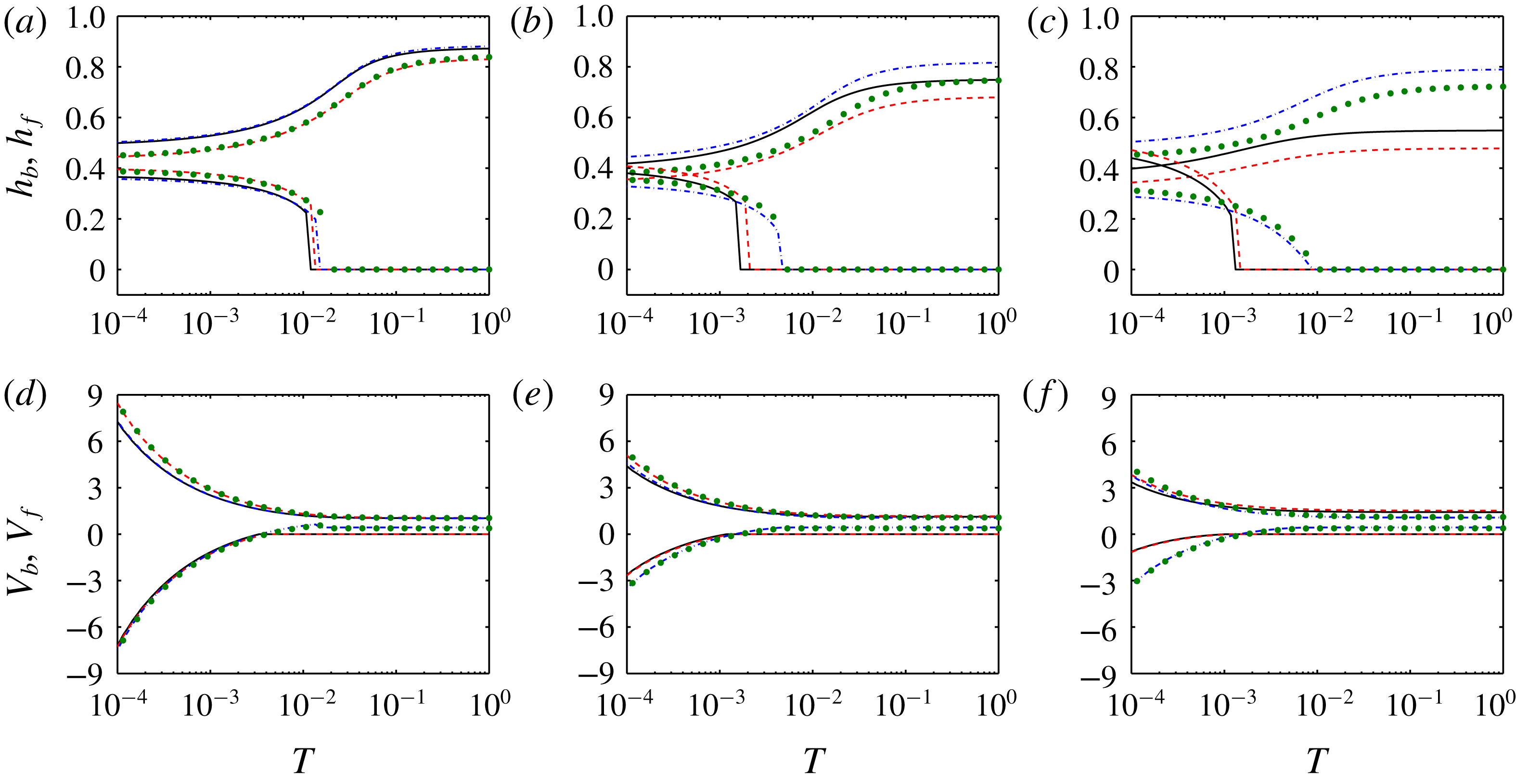
Figure 11 plots the variation of the leading and trailing front heights and speeds versus time, at $\unicode[STIX]{x1D712}=0$ , for different $m$ and the four slip cases. In general, it is observed that the leading/trailing front height increases/decreases as time grows. On the other hand, $|V_{f}|$ and $|V_{b}|$ both decrease with time. It is interesting to note that generally $|V_{f}|\neq |V_{b}|$ and that $V_{f}$ remains always positive (as expected) but $V_{b}$ crosses over between negative and positive values. In addition, $h_{f}$ and $h_{b}$ are far from symmetric with respect to $h=0.5$ . In general, it can be also said that the front heights and speeds reach their steady values as $T\sim O(10^{-1})$ . Finally, lower/higher viscosity ratios further affect the leading/trailing front velocities, which, as explained earlier, is simply to the dominance of the wall slip at the lower/upper wall.

4.6 Lock-exchange flows

Our main purpose in this paper is to study two-layer flows for which there is always an imposed flow velocity ( $\hat{V}_{0}\neq 0$ ). In this case, the model is valid for small and large values of the buoyancy number. However, an important class of problems, i.e. the lock-exchange flows, cannot be directly evaluated using the scaling presented earlier (since $\unicode[STIX]{x1D712}\rightarrow \infty$ as $\hat{V}_{0}\rightarrow 0$ ). Therefore, it is worth developing and presenting an alternative lubrication model scaling, exclusively for the case of lock-exchange flows in an inclined channel. To do so, we re-scale velocities using a characteristic velocity defined as

(4.18) $$\begin{eqnarray}\displaystyle \hat{V}_{c}\equiv \frac{(\hat{\unicode[STIX]{x1D70C}}_{H}-\hat{\unicode[STIX]{x1D70C}}_{L}){\hat{g}}D_{0}^{2}\cos \unicode[STIX]{x1D6FD}}{2\hat{\unicode[STIX]{x1D707}}_{H}}, & & \displaystyle\end{eqnarray}$$

which is simply the longitudinal component of a viscous velocity scale obtained through balancing viscous and buoyant stresses. We can therefore re-define the lubrication model parameters as

(4.19) $$\begin{eqnarray}\displaystyle \unicode[STIX]{x1D712}_{e} & = & \displaystyle 2,\end{eqnarray}$$

(4.20) $$\begin{eqnarray}\displaystyle \unicode[STIX]{x1D6FF}_{e} & = & \displaystyle \frac{\cot \unicode[STIX]{x1D6FD}}{2},\end{eqnarray}$$

(4.21) $$\begin{eqnarray}\displaystyle X_{e} & = & \displaystyle \unicode[STIX]{x1D6FF}_{e}x,\end{eqnarray}$$

(4.22) $$\begin{eqnarray}\displaystyle T_{e} & = & \displaystyle \unicode[STIX]{x1D6FF}_{e}t,\end{eqnarray}$$

(4.23) $$\begin{eqnarray}\displaystyle P_{e} & = & \displaystyle \unicode[STIX]{x1D6FF}_{e}p,\end{eqnarray}$$

(4.24) $$\begin{eqnarray}\displaystyle V_{e} & = & \displaystyle v/\unicode[STIX]{x1D6FF}_{e}.\end{eqnarray}$$

For Newtonian fluids, the definition of $m$ , $\unicode[STIX]{x1D706}_{l}$ and $\unicode[STIX]{x1D706}_{u}$ would not be affected by the alternative scaling. The lock-exchange flow flux function can be simply obtained through removing the advective component from $q_{H}$ to find

(4.25) $$\begin{eqnarray}\displaystyle q_{H,e}=q_{H,B}(\unicode[STIX]{x1D712}_{e}-h_{X_{e}}). & & \displaystyle\end{eqnarray}$$

In all the above relations, the subscript $e$ represents the lock-exchange flow case.

Figure 12.

Examples of lock-exchange interface profiles for $m=1$ and $T_{e}=0,10,\ldots ,90,100$ . For a better visualization of symmetry/asymmetry, a bold line marks the last profile (corresponding to $T_{e}=100$ ). A steep linear function, i.e. $h(X,T_{e}=0)=-10X_{e}+0.5$ , is used as the initial profile. (a) Case I; (b) Case II; (c) Case III; (d) Case IV.

Figure 12 illustrates the evolution of the lock-exchange interface profiles for the four slip cases, for an iso-viscous displacement. The interface evolution is initially faster due to a large interface slope. At longer times the interface evolution slows down and the interface steadily evolves due to the channel slope. The symmetric slip cases, i.e. Case I (no slip at either wall) and Case IV (equal slip at both walls), present a symmetric flow evolution, although the interpenetration is stronger in Case IV, as expected. The interface profiles of Cases II and III present asymmetric flows. To highlight this, the interface positions at $X_{e}=0$ are also marked by the arrows. Overall, figure 12 shows that the wall slip cases affect lock-exchange flows at both short and long times.

5.1 Static residual wall layers

Although the literature of static wall layers in viscoplastic fluid flows is expanding thanks to the recent works of Roustaei & Frigaard (Reference Roustaei and Frigaard2013), Roustaei & Frigaard (Reference Roustaei and Frigaard2015), Roustaei, Gosselin & Frigaard (Reference Roustaei, Gosselin and Frigaard2015), Mollaabbasi & Taghavi (Reference Mollaabbasi and Taghavi2016) and others, it was perhaps Allouche et al. (Reference Allouche, Frigaard and Sona2000) who pioneered a model to analyse SRWLs in viscoplastic displacement flows, for the case of a vertical channel flow (i.e. symmetric). Taghavi et al. (Reference Taghavi, Seon, Martinez and Frigaard2009) extended the work of Allouche et al. (Reference Allouche, Frigaard and Sona2000) to slumping displacements in a channel with no-slip boundary conditions. These and similar works have demonstrated that, for the cases where SRWLs exist, the maximal SRWL thickness is typically observed at longer times. Therefore, we also concentrate our analysis on long times and rely on a similar procedure proposed by Allouche et al. (Reference Allouche, Frigaard and Sona2000) and Taghavi et al. (Reference Taghavi, Seon, Martinez and Frigaard2009) to calculate our SRWL thickness for displacements with wall slip.

Below, we will systematically analyse the formation of SRWLs, for the four wall slip cases. First, we will treat Cases I and II and then extend our analysis to a marginal state for Cases III and IV.

5.1.1 Static wall layers for Cases I and II

Assuming that fluid $L$ is fully static for $y\in [h,1]$ , the governing equation for the heavy fluid motion can be written as

(5.2) $$\begin{eqnarray}\displaystyle \frac{\unicode[STIX]{x2202}}{\unicode[STIX]{x2202}y}\unicode[STIX]{x1D70F}_{H,Xy}=\frac{\unicode[STIX]{x2202}P_{0}}{\unicode[STIX]{x2202}X},\quad y\in (0,h_{s}), & & \displaystyle\end{eqnarray}$$

where $h_{s}$ is the corresponding interface height. The appropriate boundary conditions are

(5.3) $$\begin{eqnarray}\displaystyle u(0) & = & \displaystyle \unicode[STIX]{x1D706}_{l}\unicode[STIX]{x1D70F}_{H},\end{eqnarray}$$

(5.4) $$\begin{eqnarray}\displaystyle u(h_{s}) & = & \displaystyle 0.\end{eqnarray}$$

On the other hand, the flow rate condition becomes

(5.5) $$\begin{eqnarray}\displaystyle \int _{0}^{h_{s}}u(y)\,\text{d}y=1. & & \displaystyle\end{eqnarray}$$

For simplicity, let us assume that $\unicode[STIX]{x1D706}_{l}$ is small so that the plug core within the lower layer does not touch the lower wall. We then define $h_{1}$ as the vertical distance between the lower wall and the place where the shear stress becomes zero within the heavy layer (note that due to the slip at the lower wall, the velocity profile can be asymmetric within the lower layer). We simply integrate the above system to find the velocity field and then integrate across the heavy fluid layer to transform equation (5.5) into

(5.6) $$\begin{eqnarray}\displaystyle & & \displaystyle \frac{h_{s}^{2}{\tilde{B}_{H}}^{1/n_{H}}((\tilde{h}_{1}-\unicode[STIX]{x1D709})^{2+1/n_{H}}-(\tilde{h}_{1}-2)(2-\tilde{h}_{1}-\unicode[STIX]{x1D709})^{1+1/n_{H}})}{4\,\unicode[STIX]{x1D709}^{1/n_{H}}\left(2+\displaystyle \frac{1}{n_{H}}\right)}\nonumber\\ \displaystyle & & \displaystyle \quad +\,\frac{h_{s}^{2}{\tilde{B}_{H}}^{1/n_{H}}\left(\displaystyle \frac{1}{n_{H}}+3\right)(2-\tilde{h}_{1}-\unicode[STIX]{x1D709})^{1+1/n_{H}}}{4\,\unicode[STIX]{x1D709}^{1/n_{H}-1}\left(\displaystyle 1+\frac{1}{n_{H}}\right)\left(2+\displaystyle \frac{1}{n_{H}}\right)}-\frac{\tilde{h}_{1}\,\tilde{\unicode[STIX]{x1D706}}_{l}(\unicode[STIX]{x1D709}-\tilde{h}_{1})h_{s}\,\tilde{B}_{H}}{2\unicode[STIX]{x1D709}}=1,\end{eqnarray}$$

where $\tilde{B}_{H}=B_{H}/(1-B_{H})$ and $\tilde{\unicode[STIX]{x1D706}}_{l}=\unicode[STIX]{x1D706}_{l}(1-B_{H})$ , while $h_{s}$ and $\tilde{h}_{1}=2h_{1}/h_{s}$ are dependent parameters related through the solution of

(5.7) $$\begin{eqnarray}\displaystyle h_{s}=\,\frac{2{\tilde{B}_{H}}^{1-1/n_{H}}\tilde{\unicode[STIX]{x1D706}}_{l}\,\tilde{h}_{1}\left(\displaystyle 1+\frac{1}{n_{H}}\right)}{\unicode[STIX]{x1D709}^{1-1/n_{H}}((2-\tilde{h}_{1}+\unicode[STIX]{x1D709})^{1+1/n_{H}}-(\tilde{h}_{1}-\unicode[STIX]{x1D709})^{1+1/n_{H}})}. & & \displaystyle\end{eqnarray}$$

The above equation is obtained by considering the fact that one needs to find the same speed for the heavy layer plug when integrating the equations starting from the lower wall or from the interface (otherwise the plug would be deformable). Finally, $\unicode[STIX]{x1D709}$ and $\unicode[STIX]{x2202}P_{0}/\unicode[STIX]{x2202}X$ are related through

(5.8) $$\begin{eqnarray}\displaystyle -\frac{\unicode[STIX]{x2202}P_{0}}{\unicode[STIX]{x2202}X}=\frac{2B_{H}}{\unicode[STIX]{x1D709}h_{s}}. & & \displaystyle\end{eqnarray}$$

Our analysis shows that the root of (5.6), lying in $(0,1]$ , can be found numerically. In other words, $\unicode[STIX]{x1D709}$ can be found for a given set of parameters $(h_{s},\tilde{B}_{H},n_{H},\tilde{\unicode[STIX]{x1D706}}_{l})$ . Let us now suppose that $\unicode[STIX]{x1D712}$ is small so that the stress at the upper wall has the same sign as the interfacial stress. Considering that the interfacial stress is $\unicode[STIX]{x2202}P_{0}/\unicode[STIX]{x2202}X(h_{s}-h_{1})$ and the upper wall shear stress is $(1-h_{1})(\unicode[STIX]{x2202}P_{0}/\unicode[STIX]{x2202}X)+\unicode[STIX]{x1D712}(1-h_{s})$ , the initial static layer assumption is

(5.9) $$\begin{eqnarray}\displaystyle \left|(1-h_{1})\frac{\unicode[STIX]{x2202}P_{0}}{\unicode[STIX]{x2202}X}+\unicode[STIX]{x1D712}(1-h_{s})\right|\leqslant B_{L}. & & \displaystyle\end{eqnarray}$$

A maximal SRWL can be defined using the minimum of $h_{s}$ , denoted by $h_{s,min}$ , for which relation (5.9) holds:

(5.10) $$\begin{eqnarray}\displaystyle Y_{static}=1-h_{s,min}. & & \displaystyle\end{eqnarray}$$

Substituting the pressure gradient from (5.8) into (5.9), we reach at the condition governing the maximal SRWL:

(5.11) $$\begin{eqnarray}\displaystyle \frac{\tilde{B}_{Y}}{\unicode[STIX]{x1D709}}\left(\frac{2}{h_{s,min}}-\tilde{h}_{1}\right)-\tilde{\unicode[STIX]{x1D712}}(1-h_{s,min})=1, & & \displaystyle\end{eqnarray}$$

where $\tilde{B}_{Y}=B_{H}/B_{L}$ and $\tilde{\unicode[STIX]{x1D712}}=\unicode[STIX]{x1D712}/B_{L}$ . Therefore, only five parameters govern the solution of the maximal SRWL:

(5.12) $$\begin{eqnarray}\displaystyle \left.\begin{array}{@{}l@{}}\tilde{\unicode[STIX]{x1D706}}_{l},\\ \tilde{B}_{H},\\ \tilde{B}_{Y},\\ \tilde{\unicode[STIX]{x1D712}},\\ n_{H}.\end{array}\right\} & & \displaystyle\end{eqnarray}$$

In order to compare the results of the simplified method explained here and those of our numerical simulations, the horizontal dashed lines in figure 16(a,b) mark the maximal SRWL predictions, where good agreement is observed: in the simulations, the SRWL thicknesses at long times approach the predictions of the simplified method. In addition, as the heavy fluid slips at the lower wall (Case II), the SRWL thickness increases.

Figure 17.

Maximal SRWL thickness, $Y_{static}$ , with contours spaced at intervals $Y_{static}=0.1$ , for $\tilde{\unicode[STIX]{x1D712}}=n_{H}=1$ : (a) Case I with $\tilde{\unicode[STIX]{x1D706}}_{l}=0$ ; (b) Case II with $\tilde{\unicode[STIX]{x1D706}}_{l}=0.1$ . Shaded areas mark the limit where no SRWLs exist.

The critical existence condition of any SRWL is found as $h_{s,min}\rightarrow 1$ and it is given by

(5.13) $$\begin{eqnarray}\displaystyle \tilde{B}_{Y}=\frac{\unicode[STIX]{x1D709}|_{h_{s,min\rightarrow 1}}}{(2-\tilde{h}_{1})}. & & \displaystyle\end{eqnarray}$$

Figure 17 shows the variation of the maximum SRWL versus $\tilde{B}_{H}$ and $\tilde{B}_{Y}$ , for Cases I and II, at fixed values of $\tilde{\unicode[STIX]{x1D712}}$ and $n_{H}$ . The shaded area marks the region where no SRWL is found. It can be seen that, at large $\tilde{B}_{H}$ , slip at the lower wall (Case II) has two effects: reducing the region where no SRWL is possible and changing the spacing between the contours of the maximal SRWL thickness.

Figure 18.

Maximal SRWL thickness, $Y_{static}$ , with contours spaced at intervals $Y_{static}=0.1$ , for $n_{H}=1$ : (a) Case III with $\tilde{\unicode[STIX]{x1D706}}_{l}=0$ ; (b) Case IV with $\tilde{\unicode[STIX]{x1D706}}_{l}=0.1$ . For a given set of $h_{s}$ and $\tilde{B}_{H}$ , the corresponding values of $\tilde{\unicode[STIX]{x1D712}}$ can be calculated using equation (5.14). Shaded areas mark the limit where no SRWLs exist.

5.1.2 Static wall layers for Cases III and IV

Regarding Cases III and IV, SRWLs appear only if the stress at the upper wall is exactly zero and the interfacial stress is smaller than the light fluid’s yield stress. This means that the following relations need to be simultaneously satisfied to deliver the maximal SRWL thickness:

(5.14) $$\begin{eqnarray}\displaystyle \left.\begin{array}{@{}l@{}}\displaystyle \tilde{\unicode[STIX]{x1D712}}=\frac{2-h_{s,min}\tilde{h}_{1}}{h_{s,min}(2-\tilde{h}_{1})(1-h_{s,min})},\\ \displaystyle \tilde{B}_{Y}=\frac{\unicode[STIX]{x1D709}}{2-\tilde{h}_{1}}.\end{array}\right\} & & \displaystyle\end{eqnarray}$$

For a given parameter set, there exists a critical value for $\tilde{\unicode[STIX]{x1D712}}$ for which the displaced layer is fully static. Figure 18 plots the variation of the maximum SRWL in the plane of $\tilde{B}_{H}$ and $\tilde{B}_{Y}$ , for Cases III and IV, at a fixed value of $n_{H}$ . Note that, for a given set of $h_{s}$ and $\tilde{B}_{H}$ , the corresponding values of $\tilde{\unicode[STIX]{x1D712}}$ need be calculated using equation (5.14). For example, in this figure for $h_{s}=0.5$ and $\tilde{B}_{H}=6$ , the critical values of $\tilde{\unicode[STIX]{x1D712}}$ for Cases III and IV are equal to 6 and 5.3, respectively. This suggests the parameter ranges for which a SRWL is observed is sensitive to the variations of the Bingham numbers and the buoyancy number. Finally, compared to Case III, slip at both walls (Case IV) results in a further shrinkage of the region where no SRWL is possible.