1. Introduction
Hydrodynamic systems subjected to time-periodic forcing are a captivating area of study that has attracted considerable attention across various scientific disciplines, including environmental science, engineering and biophysics. This includes the dynamics of the sediments transported by unsteady flows over river/sea beds (Vittori et al. Reference Vittori, Blondeaux, Mazzuoli, Simeonov and Calantoni2020) and the behaviour of thermocapillary and buoyant flows under gravitational modulation in materials processing aboard spacecraft (Ostrach Reference Ostrach1982). These systems, which involve the interplay of fluid dynamics and external periodic forcing, display intricate and complex behaviour that is both fascinating and challenging to comprehend.
The Faraday experiment is one of the most useful prototypical configurations for time-periodically modulated systems where surface waves are parametrically excited by subjecting the fluid container to a purely sinusoidal vertical acceleration of one single component (Faraday Reference Faraday1831). The waves oscillate subharmonically when the forcing amplitude exceeds a threshold. In this experiment, patterns with different symmetries including rolls, squares, hexagons and 8,10,12-fold quasipatterns have been observed (Christiansen, Alstrøm and Levinsen Reference Christiansen, Alstrøm and Levinsen1992). By employing two-frequency forcing, these patterns becomes more readily observed and several other exotic patterns have been detected in laboratory experiments such as triangular patterns (Muller Reference Muller1993), quasipatterns (Edwards & Fauve Reference Edwards and Fauve1994; Kudrolli, Pier & Gollub Reference Kudrolli, Pier and Gollub1998) and superlattice patterns (Kudrolli et al. Reference Kudrolli, Pier and Gollub1998). The use of multiple-frequency driving alters and controls the interactions of different excited modes, as each excitation frequency can linearly excite a well-defined wave pattern with a specific wavenumber (Arbell & Fineberg Reference Arbell and Fineberg2002; Porter, Topaz & Silber Reference Porter, Topaz and Silber2004).
In thermal convection, the use of multiple-frequency gravitational modulation has been widely used by several authors as a control strategy to delay or enhance the convection threshold. In the presence of vertical quasiperiodic vibrations having two incommensurate frequencies, Boulal et al. (Reference Boulal, Aniss, Belhaq and Rand2007, Reference Boulal, Aniss, Belhaq and Azouani2008) and Boulal, Riahi and Aniss (Reference Boulal, Riahi and Aniss2024) showed that thermal instability in a horizontal Newtonian liquid layer with rigid boundaries could be stabilised or destabilised depending on the irrational frequency ratio. The influence of this type of gravitational modulation on convective instability of reaction fronts in porous media has been studied by Allali, Belhaq and Karouni (Reference Allali, Belhaq and Karouni2012). Using direct numerical simulations of the derived linear stability equations, these authors showed that, for specific values of amplitudes and frequency ratios of the quasiperiodic vibration, a stabilising effect of reaction fronts in a porous medium can be gained if the reacting fluid is heated from below. The onset of Rayleigh–Bénard convection and heat transfer under two-frequency rotation modulation has been recently investigated by Ansa and Pranesh (Reference Ansa and Pranesh2021), who concluded that two-frequency rotation modulation yields higher stability bounds and inhibits the convective heat transfer process in comparison with the unmodulated and single-frequency rotation modulation cases.
While the aforementioned papers concerned gravitational and rotational modulations, several investigations in the literature are interested in studying the effect of time-periodically varying boundary conditions (Yang et al. Reference Yang, Chong, Wang, Verzicco, Shishkina and Lohse2020; Sakine et al. Reference Sakine, Hayani Choujaa, Riahi, Daya and Aniss2022; Urban et al. Reference Urban, Hanzelka, Králik, Musilová and Skrbek2022; Riahi et al. Reference Riahi, Hayani Choujaa, Er Rajy and Aniss2024; Riahi, Hayani Choujaa & Wang Reference Riahi, Hayani Choujaa and Wang2025). Ansa & Pranesh (Reference Ansa and Pranesh2023) investigated the effect of bottom-wall two-frequency boundary temperature modulations on the onset of Rayleigh–Bénard convection and showed that the two-frequency case leads to a stabilisation of the system in comparison with the single-frequency case. This stabilisation means a suppression of the convective rolls observed at the threshold calculated in the single-frequency case. Chen, Gibson & Craven (Reference Chen, Gibson and Craven2023) studied the transport of energy between heat baths with two-frequency oscillating temperatures with commensurate ratios. It is concluded that time-periodic temperature modulations are a potential route to control energy storage and release in molecular devices and nanosystems. Recently, El Jaouahiry & Aniss (Reference El Jaouahiry and Aniss2025) performed a linear stability analysis to investigate the dynamics of a thin Newtonian fluid layer with a deformable free surface bounded at the bottom by a horizontal wall subjected to quasiperiodic forcing in its own plane. It was shown that, for a large frequency ratio and for a velocity amplitude ratio equal to unity, an alternation between instabilities of long wavelength and finite wavelength sets in. However, decreasing the frequency ratio leads to a merging phenomenon of three long/finite wavelength instability modes into one single mode.
Time-modulated Taylor–Couette flow is also one of the most useful prototypical configurations for studying time-periodically modulated systems (Riley & Laurence Reference Riley and Laurence1976; Youd, Willis & Barenghi Reference Youd, Willis and Barenghi2003; Youd & Barenghi Reference Youd and Barenghi2005; Avila et al. Reference Avila, Belisle, Lopez, Marques and Saric2008; Riahi, Aniss & Ouazzani Touhami Reference Riahi, Aniss and Ouazzani Touhami2019; Hayani Choujaa et al. Reference Hayani Choujaa, Aniss, Ouazzani Touhami, Khalid Naciri and Riahi2021; Riahi, Hayani-Choujaa & Aniss Reference Riahi, Hayani-Choujaa and Aniss2022; Hayani Choujaa, Riahi & Aniss Reference Hayani Choujaa, Riahi and Aniss2024a
). On the basis of narrow-gap linear stability analysis, Riley & Laurence (Reference Riley and Laurence1976) have shown that by slowly and periodically oscillating the inner cylinder with zero mean, the radial and axial components of the disturbance pulse in different directions on successive oscillations. This is not the case when the oscillation frequency becomes greater than a critical value where the radial and axial components have the same direction during successive pulses. After twenty-seven years, this feature has been revisited in detail on the basis of finite-gap nonlinear analysis by Youd et al. (Reference Youd, Willis and Barenghi2003) and Youd & Barenghi (Reference Youd and Barenghi2005), who demonstrated the existence of two classes of Taylor vortex flows called reversing and non-reversing flows. In the latter, taking place at relatively high frequency where the oscillation period is small, the Taylor vortices rotate in one privileged direction regardless of the change in the direction of rotation of the inner drive. This is in contrast to the reversing flow, which takes place at low frequencies, where the oscillation period is sufficient for the Taylor vortices to respect the direction of rotation of the drive. This dynamics has been revisited both experimentally and theoretically by Avila et al. (Reference Avila, Belisle, Lopez, Marques and Saric2008), who shed light on the symmetry breaking bifurcation experienced by the basic state at the onset of instability. Indeed, when the reversing flow sets in, the
 $Z_2$
spatio-temporal symmetry of the basic state is broken while it is preserved by the non-reversing flow. The effect of oscillating the outer cylinder in phase or out of phase with the same frequency as the inner cylinder was studied by Riahi et al. (Reference Riahi, Aniss and Ouazzani Touhami2019), Riahi et al. (Reference Riahi, Hayani-Choujaa and Aniss2022) and Hayani Choujaa et al. (Reference Hayani Choujaa, Riahi and Aniss2024b
), who showed that the reversing flow is sustained by the counter-oscillation which inhibits the non-reversing flow. New families of reversing and non-reversing flows were discovered by these authors by varying the relative amplitudes of the cylinders.
Time-modulated Taylor–Couette flow with two-frequency forcing has not been sufficiently studied (Ern & Wesfreid Reference Ern and Wesfreid2002; Marques, Lopez & Iranzo Reference Marques, Lopez and Iranzo2002; Riahi, Hayani Choujaa & Aniss Reference Riahi, Hayani Choujaa and Aniss2025). Ern & Wesfreid (Reference Ern and Wesfreid2002) are interested in the case where both the inner and outer cylinders are co-oscillating with the angular velocity
 $\varOmega _1 \cos (\omega _1t)+ \varOmega _2 \cos (\omega _2t)$
. These authors considered only one frequency ratio,
 $\omega _2/\omega _1 = 16$
, where
 $\omega _2 = 32$
and
 $\omega _1 = 2$
, corresponding to the case of weakly oscillating cylinders subjected to a high-frequency forcing with two commensurate frequencies. This study was conducted experimentally and theoretically using a quasi-steady analysis where time derivatives are completely neglected from the linear stability equations. This analysis is generally valid under the assumption of low-frequency forcing, and this is the reason why they considered a second high frequency, i.e.
 $\omega _2$
, with a weak amplitude such that
 $\varOmega _2/\varOmega _1 = 0.2$
. Under these assumptions, satisfactory agreement between theoretical and experimental findings is found where it is shown that the temporal behaviour of secondary flow grows and damps several times during a flow cycle. This feature was observed neither experimentally nor theoretically in the single-frequency case (Aouidef et al. Reference Aouidef, Normand, Stegner and Wesfreid1994; Aouidef & Normand Reference Aouidef and Normand1996, Reference Aouidef and Normand2000; Ern Reference Ern1998; Ern & Wesfreid Reference Ern and Wesfreid1999). When dealing with periodically forced Taylor–Couette systems in the axial direction, Marques, Lopez & Iranzo (Reference Marques, Lopez and Iranzo2002) investigated the case where the inner cylinder is rotating at constant angular velocity and oscillating in the axial direction with velocity
 $W(\sin (\bar {\omega } t) + \epsilon \sin (2\bar {\omega } t))$
(
 $W$
and
 $\bar {\omega }$
denote respectively the oscillation amplitude and the oscillation frequency of the inner cylinder in the axial direction). The outer cylinder is considered fixed. Here,
 $\epsilon$
is considered as a parameter measuring the order of magnitude of imperfections in the axial force. These authors showed that the presence of the two frequencies at a sufficiently low value of
 $\epsilon$
significantly reduces the range of validity of the generic unfolding of the gluing bifurcation of three-tori observed in the single-frequency case.
In this paper, we perform a detailed numerical study on the linear dynamics of two-frequency-modulated Taylor–Couette flow using Floquet analysis of the basic state. We consider the case where the inner and outer cylinders are oscillating with the angular velocities
 $\varOmega _{\textit{in}} = \varOmega _0 \cos (\omega _1t)$
and
 $\varOmega _{\textit{out}} = \varOmega _0 \cos (\omega _2t)$
, respectively. This flow configuration has been recently studied by Riahi, Hayani Choujaa & Aniss (Reference Riahi, Hayani Choujaa and Aniss2025), who demonstrated, at assigned values of the frequencies
 $\omega _1$
and
 $\omega _2$
, the occurrence of bursting and regular oscillations caused by interactions of two Stokes layer flows generated by each cylinder. These authors based their analysis on the growth rate of axisymmetric disturbances to correlate the occurrence of bursting oscillations with the emergence of several harmonic and subharmonic instability modes at the critical Taylor number. However, when only one instability mode is obtained we are dealing with regular modes. In the current study, we determine, over a wide range of the frequency
 $\omega _1$
, the critical instability parameters at different irrational frequency ratios
 $\omega =\omega _2/\omega _1$
with emphasis on the limiting boundaries between bursting and regular oscillations. One of the most interesting questions that we seek to answer in the present paper concerns the influence of this quasiperiodic frequency ratio on the critical instability parameters and how it could alter the reversing and non-reversing flow observed in the case
 $\omega = 1$
. Also, we attempt to shed light on the physical mechanisms behind the growing and damping behaviour that occurred several times during a flow cycle in Ern and Wesfried’s experiment (Ern & Wesfreid Reference Ern and Wesfreid2002).
The paper is organised as follows. Section 2 deals with a description of the mathematical equation related to the basic state and its linear stability analysis taking into account three-dimensional disturbances. The numerical procedure is presented in § 3. In § 4, the results stemming from the Floquet analysis of the basic state are presented in the cases of axisymmetric and non-axisymmetric disturbances. The asymptotic low-frequency behaviour of the system is investigated on the basis of a local quasi-steady analysis and Rayleigh discriminant detailed in § 5 while § 6 is devoted to the conclusion.
2. Base flow and linear stability problem
Consider a Newtonian fluid layer with kinematic viscosity
 $\nu$
and density
 $\rho$
filling the gap between two concentric and infinitely long cylinders of radii
 $R_1$
and
 $R_2 = R_1 + d$
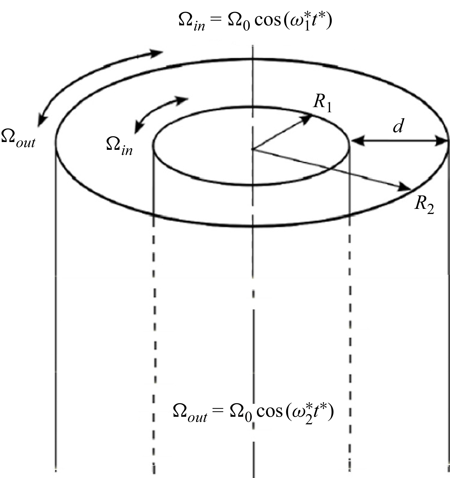
. The inner and outer cylinders are oscillating about zero mean with the angular velocities
 $\varOmega _{\textit{in}} = \varOmega _0 \cos (\omega ^*_1 t^*)$
and
 $\varOmega _{\textit{out}} = \varOmega _0 \cos (\omega ^*_2 t^*)$
, respectively. The quantities
 $\varOmega _0$
and
 $t^*$
denote respectively the modulation amplitude and the dimensional time while
 $\omega ^*_1$
and
 $\omega ^*_2$
represent respectively the dimensional modulation frequencies of the inner and outer cylinders (see figure 1). Under these conditions, the dynamics of the system becomes dependent on three time scales given by the viscous diffusive time of the fluid,
 $\tau _v = d^2/\nu$
and the dimensional modulation periods
 $T^*_1$
and
 $T^*_2$
related to the inner and outer cylinders, respectively.
Sketch of the geometry.

Assuming that the gap width
 $d$
between the cylinders is small compared with the radius
 $R_1$
and using the small-gap approximation in which all terms of order
 $\varepsilon = d/R_1$
are generally neglected except those multiplied by a control parameter. In this case, the time-dependent velocity of the purely azimuthal base flow satisfies the following equation:
 \begin{equation} \dfrac {\partial\! V_{\!B}}{\partial t} = \dfrac {\partial ^2\! V_{\!B}}{\partial x^2}, \end{equation}
with the boundary conditions
 \begin{equation} V_{\!B} (x = 0,t)= \cos (\omega _1 t)\,\,\,\,\mbox{and}\,\,\,\,V_{\!B} (x = 1,t)= \cos (\omega _2 t), \end{equation}
while the base pressure field
 $P_{\!B}$
is determined by the equation
 \begin{equation} \frac {\partial\! P_{\!B}}{\partial x} = \varepsilon \textit{Re} V_{\!B}^2, \end{equation}
where
 $x$
is the radial coordinate related to the dimensional radial one,
 $r$
, by:
 $r = x d + R_1$
. This dimensionless form is obtained by using
 $d^2/\nu$
,
 $R_1\varOmega _0$
and
 $\rho R_1\varOmega _0 \nu /d$
as the time, azimuthal velocity and pressure scales respectively. Within this context, curvature effects are involved only in the pressure field through the centrifugal force term of order
 $\varepsilon Re$
, by requiring that the Reynolds number,
 $Re = R_1\varOmega _0 d/\nu$
, be held fixed as
 $\varepsilon \to 0$
. However, curvature effects are entirely neglected in the velocity field, which is reminiscent of the velocity field of flows between two oscillating plates. It is worth noting that the parameters
 $\omega _1$
and
 $\omega _2$
represent respectively the dimensionless frequencies of the inner and outer cylinders. Each frequency represents the ratio between the viscous diffusive time,
 $\tau _v$
, and the dimensional modulation periods, denoted
 $T^*_1$
and
 $T^*_2$
, where
 $\omega _1 = 2\pi \tau _v/T^*_1 = \omega ^*_1 d^2/ \nu$
and
 $\omega _2 = 2\pi \tau _v/T^*_2 = \omega ^*_2 d^2/\nu$
.
The solution of (2.1) associated with the boundary conditions (2.2) is written as the superposition of two velocity profiles. The first one corresponds to the flow generated by the oscillation of the inner cylinder, designated by
 $V_{B1}$
, while the second one is that of the outer one designated by
 $V_{B2}$
. The expression of
 $V_{\!B} (x, t)$
is then given by
 \begin{equation} V_{\!B} (x,t)= \sum _{i=1}^{2} V_\textit{Bi} (x, t), \end{equation}
where
 \begin{equation} V_\textit{Bi} (x,t)= V_{1i} (x) \cos (\omega _i t) + V_{2i} (x) \sin (\omega _i t), \end{equation}
and the functions
 $V_{1i}$
and
 $V_{2i}$
are given by
 \begin{align} V_{11} (x)=\frac {\cos (\gamma _1 x)\cosh (\gamma _1 (1-x))\cosh (\gamma _1)- \cos (\gamma _1 (1-x))\cosh (\gamma _1 x)\cos (\gamma _1)}{\cosh ^2(\gamma _1) - \cos ^2(\gamma _1 )}, \end{align}
 \begin{align} V_{12} (x)=\frac {\cos (\gamma _2 (1-x))\cosh (\gamma _2 x)\cosh (\gamma _2)- \cos (\gamma _2 x)\cosh (\gamma _2 (1-x))\cos (\gamma _2)}{\cosh ^2(\gamma _2) - \cos ^2(\gamma _2)}, \end{align}
 \begin{align} V_{21} (x)=\frac {\sin (\gamma _1 x)\sinh (\gamma _1 (1-x))\cosh (\gamma _1)- \sin (\gamma _1 (1-x))\sinh (\gamma _1 x)\cos (\gamma _1)}{\cosh ^2(\gamma _1) - \cos ^2(\gamma _1 )}, \end{align}
 \begin{align} V_{22} (x)=\frac {\sin (\gamma _2 (1-x))\sinh (\gamma _2 x)\cosh (\gamma _2 )-\sin (\gamma _2 x)\sinh (\gamma _2 (1-x))\cos (\gamma _2)}{\cosh ^2(\gamma _2) - \cos ^2(\gamma _2)}. \end{align}
This basic state consists of two viscous waves generated by the oscillating inner and outer cylinders. These waves penetrate the gap between the cylinders at a distance of the order of the (dimensional) Stokes layer given by
 $\delta _{1} = \sqrt {2\nu /\omega _1^*}$
for the wave generated by the inner cylinder and
 $\delta _{2} = \sqrt {2\nu /\omega _2^*}$
for the wave generated by the outer one. In addition, the naturally appearing parameter
 $\gamma _1 = \sqrt {\omega _1/2}$
(
 $\gamma _2 = \sqrt {\omega _2/2}$
) is defined as the ratio of two characteristic lengths
 $d$
and
 $\delta _{1}$
(
 $\delta _{2}$
), i.e.
 $\gamma _1 = d/\delta _{1}$
(
 $\gamma _2 = d/\delta _{2}$
).
The ratio between the frequencies represents the ratio between the two-dimensional thicknesses of the inner and outer boundary Stokes layers squared, i.e.
 $\omega _2/\omega _1 = (\delta _{2}/\delta _{1})^2$
. This ratio represents in addition the ratio between the period of the driving force applied to the inner and outer cylinders, i.e.
 $\omega _2/\omega _1 = T_1/T_2$
. Here,
 $T_1$
and
 $T_2$
denote respectively a dimensional form of the modulation periods of the inner and outer cylinders respectively,
 $T_1 = T^*_1/\tau _v = 2\pi /\omega _1$
and
 $T_2 = T^*_2/\tau _v = 2\pi /\omega _2$
.
Once the base flow is determined, its linear stability with respect to three-dimensional non-axisymmetric disturbances is considered. A small perturbation field
 \begin{equation} (\tilde {\boldsymbol {u}}, \tilde {p})= \left (\hat {u}_r(x, t), \hat {u}_\theta (x, t), \hat {u}_z (x, t), \hat {p}(x, t) \right )e^{i(qz + m\theta )} \end{equation}
superimposing the base state
 $(0, V_{\!B}, 0, P_{\!B})$
is then introduced. The velocity and pressure fields in the perturbed state are written as
 \begin{equation} (u_r, u_\theta , u_z, p)= (0, V_{\!B}, 0, P_{\!B}) + (\tilde {\boldsymbol {u}}, \tilde {p}). \end{equation}
Here,
 $q$
is the axial wavenumber that is related to the wavelength
 $\tilde {\lambda }$
, i.e. the size of two counter-rotating vortices in the radial–axial plane of the geometry, by
 $\tilde {\lambda }=2 \pi /q$
, whereas
 $m$
is the azimuthal wavenumber. Since
 $\theta \in [0, 2\pi ]$
,
 $m$
is considered as an integer, in contrast to
 $q$
, which is real owing to the infinite length of the cylinders. It is worth noting that these perturbations are considered spatially periodic along the axial and azimuthal directions. In this framework, we are dealing with a three-directional time-dependent perturbed flow. By substituting the expression (2.11) into the Navier–Stokes and continuity equations, a linearisation in the perturbation quantities yields the following linear partial differential equations:
 \begin{align} & \left (M - \frac {\partial }{\partial t} - i\varepsilon \textit{mReV}_{\!B} \right ) \hat {u}_r-2\varepsilon \textit{Re}\! \left (i\varepsilon m-\textit{Re} V_{\!B}\right )\hat {u}_\theta = \textit{Re} \frac {\partial \hat {p}}{\partial x} , \end{align}
 \begin{align} &\left (M - \frac {\partial }{\partial t} - i\varepsilon \textit{mReV}_{\!B} \right ) \hat {u}_\theta -\frac {\partial V_{\!B}}{\partial x}\hat {u}_r = 0 , \end{align}
 \begin{align} & \left (M - \frac {\partial }{\partial t} - i\varepsilon \textit{mReV}_{\!B} \right )\hat {u}_z = \textit{iqRe}\hat {p} , \end{align}
 \begin{align} & \frac {\partial }{\partial x}\hat {u}_r+i\varepsilon \textit{mRe}\hat {u}_\theta +iq\hat {u}_z=0 , \end{align}
where
 $M = ( {{\partial }^2}/{{\partial x}^2})-q^2$
. The radial and axial velocities,
 $\tilde {u}_r$
and
 $\tilde {u}_z$
, are scaled by
 $\nu /d$
whereas the azimuthal one and pressure are scaled by
 $R_1 \varOmega _0$
and
 $\rho \nu R_1 \varOmega _0/d$
, respectively. It is important to point out that this stability system is obtained using the small-gap approximation where all terms of order
 $\varepsilon = d/R_1$
or higher are neglected except those multiplied by the Reynolds number. By considering non-axisymmetric disturbances, curvature effects become more significant in the stability equations, where terms of order
 $\varepsilon m$
are retained. Following Duck & Hall (Reference Duck and Hall1981) in studying the centrifugal instability of an infinite Stokes layer to non-axisymmetric disturbances, we introduce the quantity
 $k$
defined by
 \begin{equation} k = m\varepsilon ^{1/2}, \end{equation}
and consider the narrow-gap limit where
 $\varepsilon ^{1/2} \to 0$
while keeping
 $k$
fixed. Owing to the flow periodicity in the azimuthal direction, it is evident that the values of
 $k$
corresponding to non-integer values of
 $m$
have no physical relevance. After eliminating the pressure and the axial velocity, the evolution equations for amplitudes of the radial and azimuthal velocity (
 $\hat {u}_r, \hat {u}_\theta$
) components, linearised around the basic state, are given by the following linear partial differential equations:
 \begin{align} &\left (M-\frac {\partial }{\partial t} - \textit{ik}\mathit{Ta}V_{\!B} \right )M\hat {u}_r + \textit{ik}\mathit{Ta} \frac {\partial ^2 V_{\!B}}{\partial x^2}\hat {u}_r = 2 q^2 \mathit{Ta} ^2 V_{\!B} \hat {u}_\theta , \end{align}
 \begin{align} &\left (M-\frac {\partial }{\partial t} - \textit{ik}\mathit{Ta}V_{\!B} \right )\hat {u}_\theta =\frac {\partial V_{\!B}}{\partial x}\hat {u}_r , \end{align}
with the boundary conditions
 \begin{equation} \hat {u}_r=\hat {u}_\theta =\frac {\partial \hat {u}_r}{\partial x}=0\,\,\,\,\,\,\mbox{at}\,\,\,x=0\,\,\,\,\mbox{and}\,\,\,\,x=1, \end{equation}
where the Taylor number,
 $\mathit{Ta}$
, defined as
 \begin{equation} \mathit{Ta} = \mathit{Re}\sqrt {\varepsilon } = \frac {R_1 \varOmega _0 d}{\nu }\sqrt {\dfrac {d}{R_1}}, \end{equation}
represents the ratio of the centrifugal velocity
 $R_1 \varOmega _0$
and the viscous velocity
 $\nu /d$
in rotating flows with curvature, incorporated via the quantity
 $\sqrt {\varepsilon }$
. Instability sets in when the destabilising centrifugal force becomes greater than the stabilising viscous one. At a critical value of this dimensionless number,
 $\mathit{Ta_c}$
, also called a critical instability onset, time-dependent Taylor vortices emerge and their spatial structure is characterised by both the axial and azimuthal wavenumbers calculated at
 $\mathit{Ta_c}$
.
At
 $k = 0$
, we recover the stability system related to axisymmetric disturbances (Aouidef et al. Reference Aouidef, Normand, Stegner and Wesfreid1994) where curvature effects are retained solely through the Taylor number expression. However, by neglecting the time derivatives in the system (2.17)–(2.18), we recover the stability equations obtained by Krueger, Gross & Di Prima (Reference Krueger, Gross and Di Prima1966) in the case of steadily rotating cylinders. In this case, it is important to mention that the term
 $\textit{ik}\mathit{Ta} ({\partial ^2 V_{\!B}}/{\partial x^2})\hat {u}_r$
vanishes owing to the linear nature of the base flow velocity profile in this flow configuration.
When dealing with hydrodynamic systems subject to two-frequency forcing, it is more convenient to study their dynamics on the basis of the frequency ratio. The latter appears in the basic velocity expression by using the following change of variable:
 $\tau = \omega _1 t$
and the stability system becomes
 \begin{align} &\left (M-\omega _1\frac {\partial }{\partial \tau } - \textit{ik}\mathit{Ta}V_{\!B} \right )M\hat {u}_r + \textit{ik}\mathit{Ta} \frac {\partial ^2 V_{\!B}}{\partial x^2}\hat {u}_r = 2 q^2 \mathit{Ta} ^2 V_{\!B} \hat {u}_\theta , \end{align}
 \begin{align} &\left (M-\omega _1\frac {\partial }{\partial \tau } - \textit{ik}\mathit{Ta}V_{\!B} \right )\hat {u}_\theta =\frac {\partial V_{\!B}}{\partial x}\hat {u}_r. \end{align}
In this case, the components of the base flow expression are written as
 \begin{align} &V_{B1} (x,\tau )= V_{11} (x) \cos (\tau ) + V_{21} (x) \sin ( \tau ), \end{align}
 \begin{align} &V_{B2} (x,\tau )= V_{12} (x) \cos (\omega \tau ) + V_{22} (x) \sin (\omega \tau ). \end{align}
This base flow varies synchronously with the imposed harmonic forcing applied to the cylinders if and only if
 $\omega _2 = \tilde {k}\,\omega _1$
with
 $ \tilde {k} \in Q$
. The system is considered
 $2\pi$
-periodic and therefore a Floquet analysis is convenient to investigate its dynamics in light of the parameter
 $\omega$
. This periodicity is broken if the frequencies
 $\omega _1$
and
 $\omega _2$
are incommensurates, meaning that their ratio
 $\omega$
is irrational,
 $\omega \in R/Q$
. The system thus undergoes a quasiperiodic forcing and one can have recourse to the balance harmonic method or direct numerical simulations. Consequently, the use of Floquet theory is no longer efficient unless the irrational number can be approached by a rational one. Indeed, for an irrational value of
 $\omega$
there exist two relatively prime integers
 $\tilde {p}$
and
 $\tilde {q}$
such that
 $\omega = {\tilde {p}}/{\tilde {q}}$
. In this framework, using the following change of variable:
 $\tau = 2\tilde {q} \tau '$
, the final stability system is written as
 \begin{align} &\left (M-\dfrac {\omega _1}{2\tilde {q}}\frac {\partial }{\partial \tau '} - \textit{ik}\mathit{Ta}V_{\!B} \right )M\hat {u}_r + \textit{ik}\mathit{Ta} \frac {\partial ^2 V_{\!B}}{\partial x^2}\hat {u}_r = 2 q^2 \mathit{Ta} ^2 V_{\!B} \hat {u}_\theta , \end{align}
 \begin{align} &\left (M-\dfrac {\omega _1}{2\tilde {q}}\frac {\partial }{\partial \tau '} - \textit{ik}\mathit{Ta}V_{\!B} \right )\hat {u}_\theta =\frac {\partial V_{\!B}}{\partial x}\hat {u}_r , \end{align}
where the components of the base flow expression in turn are rewritten as
 \begin{align} &V_{B1} (x,\tau ')= V_{11} (x) \cos (2 \tilde {q}\tau ') + V_{21} (x) \sin (2\tilde {q} \tau '),\\[-12pt]\nonumber \end{align}
 \begin{align} &V_{B2} (x,\tau ')= V_{12} (x) \cos (2\tilde {p}\tau ') + V_{22} (x) \sin (2\tilde {p}\tau '). \end{align}
Under these assumptions, the partial differential system (2.25)–(2.26) is time periodic and therefore the use of Floquet theory becomes convenient. The validity of this numerical approach has been sufficiently proved in Riahi et al. (Reference Riahi, Hayani Choujaa and Aniss2025) since it reproduces quite well results obtained by direct numerical simulations considering irrational frequency ratios.
This procedure has been adopted recently by El Jaouahiry & Aniss (Reference El Jaouahiry and Aniss2025), who investigated the stability of a fluid layer with a deformable free surface bounded at the bottom by a horizontal wall subjected to quasiperiodic oscillation in its own plane and also by Yagoubi & Aniss (Reference Yagoubi and Aniss2017), who were interested in studying the effect of vertical quasiperiodic vibrations on the stability of the free surface of a fluid layer. The results stemming from the harmonic balance method reproduced quite well those obtained from a Floquet analysis using the same approach adopted in this paper, which consists of approaching an irrational number by a rational one.
3. Numerical approach: spatial discretisation and Floquet analysis
The stability of the system under consideration will be discussed in light of the critical instability parameters,
 $\mathit{Ta}_c$
,
 $q_c$
and
 $m_c$
(
 $k_c$
). These parameters are determined by a numerical resolution of the governing system (2.25)–(2.28) associated with their boundary conditions (2.19) using a standard method combining both the Chebyshev spectral collocation method and Floquet theory. The Chebyshev collocation spectral method is used to treat the spatial dependence using the Chebyshev functions written at
 $N$
Chebyshev collocation points (see Appendix A). Within this framework, a finite matrix equation written in the form of a Floquet system can be obtained
 \begin{equation} \overline {\overline {\mathrm{B}}}\frac {\partial }{\partial \tau '}\widehat {\mathrm{\boldsymbol {X}}}=\overline {\overline {\mathrm{M}}}\left (t\right )\widehat {\mathrm{\boldsymbol {X}}}, \end{equation}
where the state vector
 $\widehat {\boldsymbol{\mathrm{X}}}$
consists of an arrangement of the Chebyshev coefficients
 ${\widehat {\boldsymbol{\mathrm{X}}}}^t= (\hat {u}_{r_1}, \hat {u}_{r_2},\ldots .,\hat {u}_{r_N}, \hat {u}_{\theta _1}, \hat {u}_{\theta _2},\ldots .,\hat {u}_{\theta _N} )$
and
 $\overline {\overline {\mathrm{M}}}(\tau ') =\boldsymbol {M}_0 +\boldsymbol {M}_{c_1} \cos (2\tilde {q} \tau ') + \boldsymbol {M}_{s_1} \sin (2\tilde {q} \tau ') +\boldsymbol {M}_{c_2} \cos (2\tilde {p} \tau ') + \boldsymbol {M}_{s_2} \sin (2\tilde {p} \tau ')$
is a time-periodic matrix whereas
 $\overline {\overline {\mathrm{B}}}$
,
 $\boldsymbol {M}_0$
,
 $\boldsymbol {M}_{c_1}$
,
 $\boldsymbol {M}_{c_2}$
,
 $\boldsymbol {M}_{s_1}$
and
 $\boldsymbol {M}_{s_2}$
are constant coefficient matrices.
We apply the Floquet theory Nayfeh & Mook (Reference Nayfeh and Mook1979) to the discretised matrix system (3.1) which is
 $\pi$
-periodic in time. This theory then suggests the existence a constant matrix
 $\boldsymbol {R}$
, called a monodromy matrix, such that
 \begin{eqnarray} \boldsymbol {S}(\tau ' + \pi )=\boldsymbol {R}\boldsymbol {S}(\tau ') ,\end{eqnarray}
where S is the fundamental solution matrix for the system (3.1) satisfying
 \begin{equation} \boldsymbol {B}\frac {\partial \boldsymbol {S}}{\partial t}=(\boldsymbol {A} +\boldsymbol {B}_1 \cos (2\tilde {q} \tau ') + \boldsymbol {C}_1 \sin (2\tilde {q} \tau ') +\boldsymbol {B}_2 \cos (2\tilde {p} \tau ') + \boldsymbol {C}_2 \sin (2\tilde {p} \tau '))\,\boldsymbol {S}. \end{equation}
In addition, the eigenvalues of the matrix
R
,
 $\mu$
, also called Floquet multipliers and calculated using the MATLAB eig routine, allow us to determine the Floquet exponents
 $\lambda$
where
 \begin{eqnarray} \lambda _{\!j}=\frac {1}{\pi }\ln (\mu _{\!j}). \end{eqnarray}
To calculate
 $\lambda _{\!j}$
, we first determine the matrix
 $\boldsymbol {R}$
using the relation (3.2) to obtain
 \begin{eqnarray} \boldsymbol {S}(T)=\boldsymbol {R}\,\boldsymbol {S}(0). \end{eqnarray}
Thus,
 $\boldsymbol {R}$
is calculated using a fourth-order Runge–Kutta numerical scheme for the integration of the system (3.3) over one period with the initial condition
 $\boldsymbol {S}(0)=\boldsymbol {I}$
, where
 $\boldsymbol {I}$
is the identity matrix.
Change of stability occurs when one or more eigenvalues have unit modulus; this can occur in three generic ways. Indeed, the instability mode is determined by identifying the eigenvalue with the largest real part of the Floquet exponent denoted by
 $\lambda _r$
(temporal growth rate). The stability of the base flow depends on the sign of the real part,
 $\lambda _r$
. If
 $\lambda _r\gt 0$
, the flow is unstable and if
 $\lambda _r \lt 0$
, the flow is stable. Three types of solutions are expected: harmonic, subharmonic and quasiperiodic. The first and second ones correspond to the case where the Floquet multiplier is purely real whereas the quasiperiodic solutions (Hayani Choujaa et al. Reference Hayani Choujaa, Riahi and Aniss2024b
, Reference Hayani Choujaa, Riahi and Aniss2025, Reference Hayani Choujaa, Riahi and Aniss2026) correspond to the case where a pair of complex-conjugate eigenvalues cross the unit circle.
4. Results
The results presented in this paper will be discussed in light of the mode competition observed in the single-frequency case. Indeed, when the cylinders are co-oscillating with the same frequency, i.e.
 $\varOmega _{\textit{in}} = \varOmega _{\textit{out}} = \varOmega _0 \cos (\omega ^* t^*)$
and
 $\omega = 1$
(Riahi et al. Reference Riahi, Aniss and Ouazzani Touhami2019), the system exhibits two classes of axisymmetric time-periodic flows termed ‘reversing’ and ‘non-reversing’ Taylor vortex flows. Their relative dominance depends on the oscillation frequency of the cylinders, denoted by the parameter
 $\gamma$
, where
 $\gamma = \sqrt {\omega ^* d^2/2\nu }$
. Indeed, reversing Taylor vortices emerge when the driving period becomes larger than
 $0.3$
times the viscous time corresponding to
 $\gamma \prec 1.3$
in contrast to the non-reversing Taylor vortices that set in when
 $\gamma \succ 1.3$
. In addition, the presence of these flows gives rise to a discontinuity in the evolution of both the first derivative of the critical Taylor number and the critical wavenumber versus the oscillation frequency at
 $\gamma = 1.5$
(Riahi et al. Reference Riahi, Aniss and Ouazzani Touhami2019). At this latter, the system exhibits a codimension-two bifurcation point and a bi-critical state arises between these flows. These flow reversal properties are altered by the presence of the irrational nature of the frequency number
 $\omega$
, as will be shown in the present paper. What happens when the cylinders are oscillating with two incommensurate frequencies,
 $\omega \in R/Q$
? Does this quasiperiodic frequency ratio trigger other instability modes besides the known reversing and the non-reversing flows observed in the case
 $\omega = 1$
? Are there any other bi-critical states involved in the system on varying
 $\omega$
? These questions among others are answered in the framework of this section. On the other hand, we shed light on the effects produced by the quasiperiodicity (presented in term of the parameter
 $\omega$
) on the stability characteristics of the system including evolution of the critical Taylor number and the wavenumber versus the oscillation frequency. We recall here that when
 $\omega = 1$
our numerical computations reproduce quite well the experimental findings of Aouidef et al. (Reference Aouidef, Normand, Stegner and Wesfreid1994), who showed that the system is potentially unstable at the frequency number
 $\gamma = \gamma _p = 2$
and the critical Taylor number tends to infinity at the low and high oscillation frequencies. It is interesting to point out here that this
 $\gamma _p$
value corresponds to the case where the inner and outer Stokes layer thicknesses areequal to half the gap
 $\delta = d/2$
. However, when the cylinders are oscillating with different frequencies (
 $\gamma _1$
and
 $\gamma _2$
), we are dealing with two different Stokes layer thicknesses, i.e.
 $\delta _1 = d/\gamma _1$
and
 $\delta _2 = d/\gamma _2$
. If the system remains potentially unstable by varying the frequency ratio
 $\omega$
, two frequencies, i.e.
 $\gamma _{1p}$
and
 $\gamma _{2p}$
, and their corresponding
 $\delta _1$
and
 $\delta _2$
are to be determined,
 $\delta _1 = d/\gamma _{1p}$
and
 $\delta _2 = d/\gamma _{2p}$
. This question will be also elucidated in this section.
4.1. Correlation between bursters and topology of marginal stability curves
Based on the linear growth rate of axisymmetric disturbances, i.e.
 $m = 0$
 $(k_c = 0)$
, Riahi et al. (Reference Riahi, Hayani Choujaa and Aniss2025) have noticed the presence of bursters near codimension-two bifurcation points where more than one instability mode co-exist and compete at the critical onset of the primary bifurcation. The presence of these multitude of instability modes gives rise to rough growth rate evolution versus the axial wavenumber, which is not the case when dealing with regular instability modes where unimodal and smooth growth rate evolutions are observed. Does the burster nature of the primary instability mode alter the topology of the marginal stability curves ? This is the main question that we aim to highlight in this subsection.
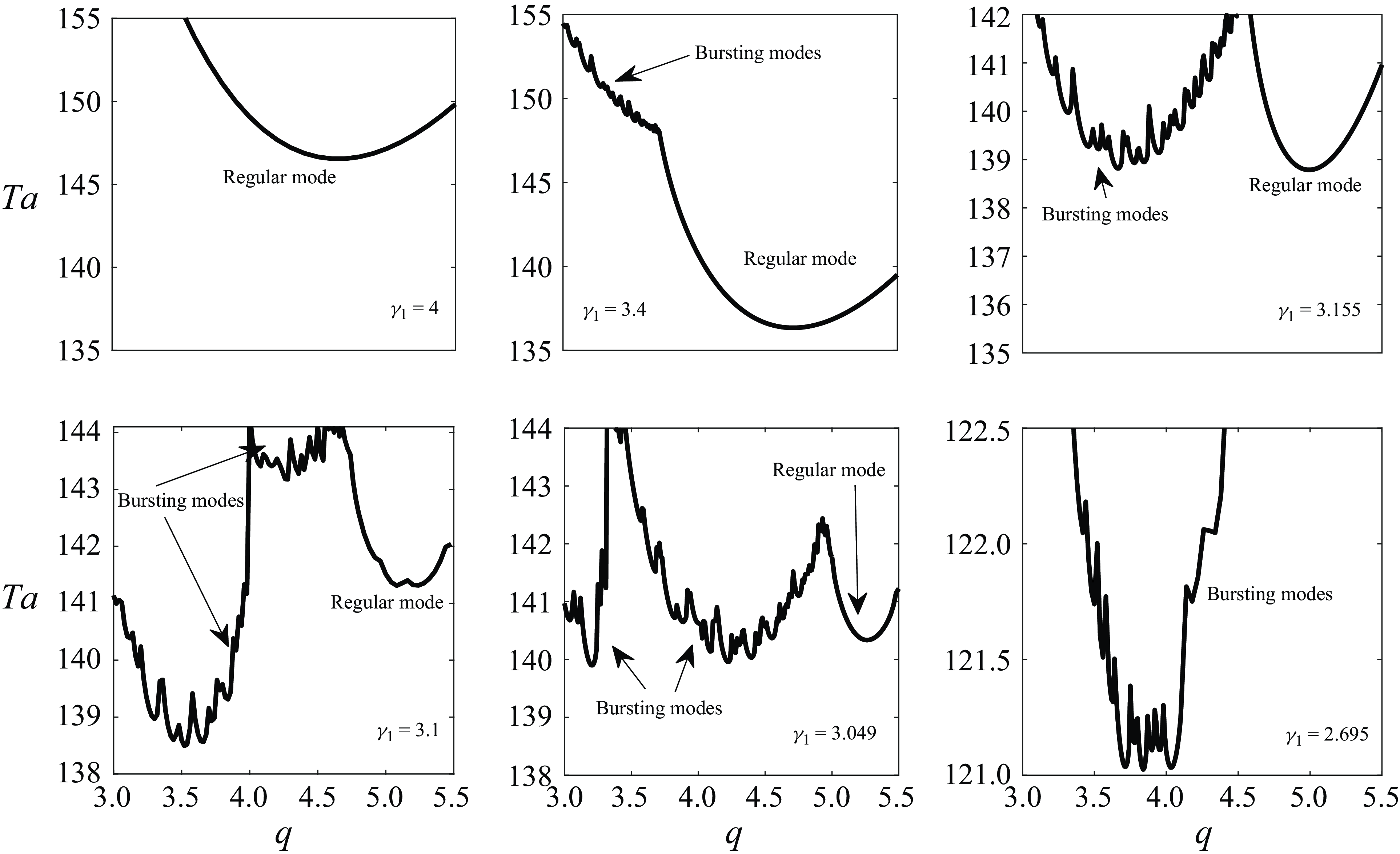
Marginal stability curves computed using Floquet theory showing the apparition of new flow states and bicritical states under the effect of the frequency
 $\gamma _1$
in the case where
 $\omega = \sqrt {3}$
. On each curve, the vertical axis is the Taylor number
 $\mathit{Ta}$
while the horizontal one is the dimensionless axial wavenumber
 $q$
, ranging from 3 to 5.5.

For this purpose, marginal stability curves are depicted in figure 2 at
 $\omega = \sqrt {3} \approx 97/56$
and different values of the frequency
 $\gamma _1$
. As one notices, only smooth, regular and uni-modal marginal stability curves are obtained when
 $\gamma _1 \succcurlyeq 4$
in contrast to the case
 $\gamma _1 = 3.4$
where finger-like features appear on a low wavenumber branch. The latter becomes more evident and parabolic at
 $\gamma _1 = 3.155$
where a codimension-two bifurcation point is detected, corresponding to a bicritical state between smooth and rough branches. Indeed, the smooth branch corresponds to a regular non-reversing instability mode, whose numerical characterisation has been carried out recently by Riahi et al. (Reference Riahi, Hayani Choujaa and Aniss2025) at
 $\gamma _1 = 10$
, whereas the rough one corresponds to a family of bursting modes. Such roughness is a physical feature that indicates the existence of numerous instability modes close to each other, clustered in a specific marginal stability branch. Such roughness concerns also the growth rate of the perturbations, as was recently shown by Riahi et al. (Reference Riahi, Hayani Choujaa and Aniss2025) when dealing with the bursting mode discussed at
 $\gamma = 3.1$
, which belongs to the rough branch in the marginal stability curve presented in figure 2. This feature sheds light on the existence of a strong correlation between the topology of the marginal stability curves and the nature of the bifurcated solution, whether it corresponds to a regular or bursting mode: smooth marginal stability curves correspond to regular instability modes whereas bursting modes correspond to rough marginal curves. It is interesting to note here that such a bursting phenomenon requires a very small wavenumber increment to be adequately elucidated because even a small uncertainty in the selection of the critical wavenumber could lead to incorrect identification of the most dangerous mode on rough branches of marginal stability curves.
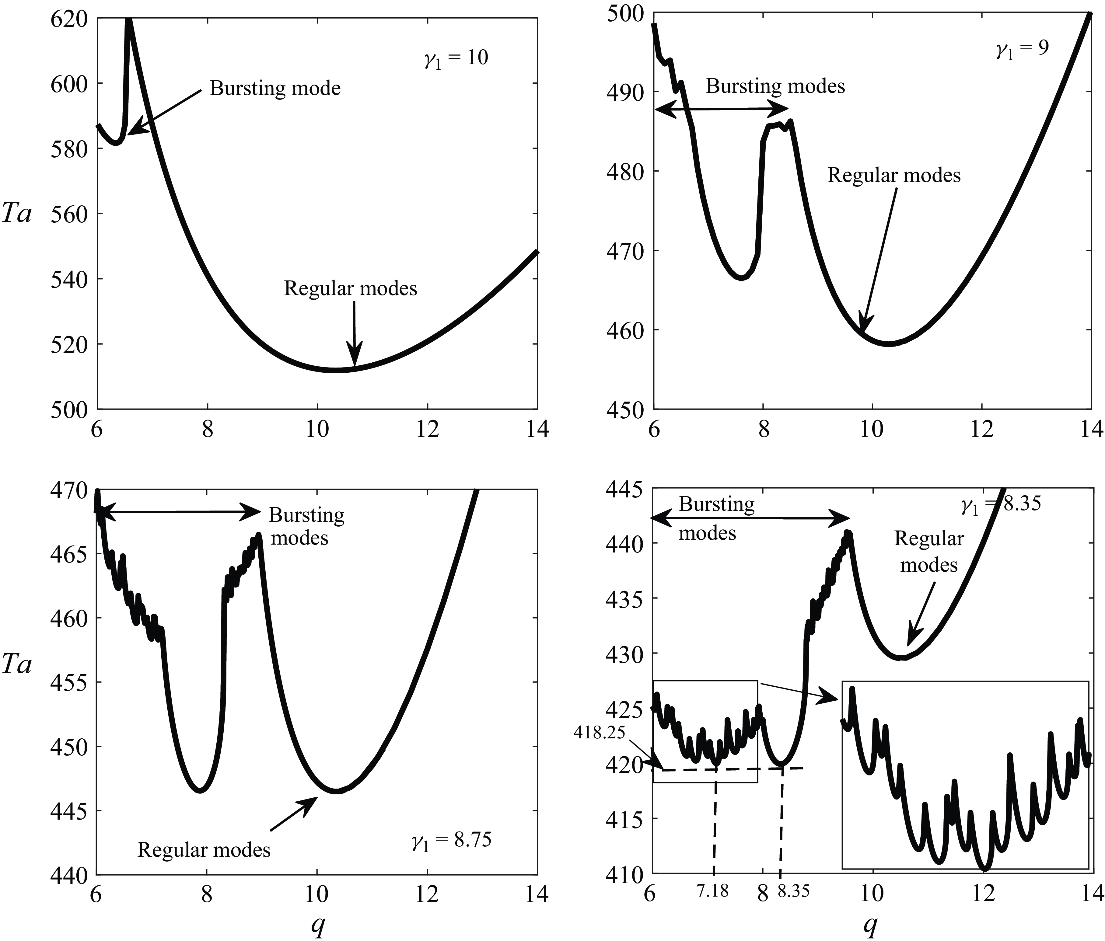
Marginal stability curves computed using Floquet theory, showing the apparition of new flow states and bicritical states under the effect of the frequency
 $\gamma _1$
in the case where
 $\omega = 1/\sqrt {37}$
. On each curve, the vertical axis is the Taylor number
 $\mathit{Ta}$
while the horizontal one is the dimensionless axial wavenumber
 $q$
, ranging from 6 to 14.

A further decrease in the frequency parameter
 $\gamma _1$
suppresses the smooth instability branch, while other rough branches appear. The dynamics of the system becomes subsequently rich and complex in the sense that each rough instability branch is composed of numerous sub-branches and consequently several codimension-two bifurcation points arise. This results in discontinuities in the axial wavenumber evolution versus the frequency number. The frequency step in these numerical calculations has to be slowly and carefully varied owing to the strong competition between numerous harmonic and subharmonic instability modes.
For the case
 $\omega \prec 1$
and by considering
 $\omega = 1/\sqrt {37} \approx 12/37$
, strong mode competition is observed at sufficiently high frequencies. This feature is illustrated in figure 3, presenting examples of marginal stability curves obtained at
 $\omega = 1/\sqrt {37}$
and some representative values of the frequency
 $\gamma _1$
. As one can see, two smooth instability branches emerge at
 $\gamma _1 = 10$
. The most unstable mode is a regular non-reversing mode, as demonstrated by Riahi et al. (Reference Riahi, Hayani Choujaa and Aniss2025) at this frequency, reached by crossing
 $\mathit{Ta}_c = 511.868$
and
 $q_c = 10.3$
while the second one is a bursting mode. This bursting mode is represented by a smooth, narrow portion of a stability curve belonging to a rough stability branch. Such roughness is evident as the oscillation frequencies of the cylinders, i.e.
 $\gamma _1$
and
 $\gamma _2$
, diminish. In this case, the first high-frequency codimension-two bifurcation point occurs at
 $\gamma _1 = 8.75$
where the primary bifurcation switches from a harmonic regular non-reversing Taylor vortex flow emerging in the frequency interval
 $\gamma _1 \succ 8.75$
to a bursting harmonic reversing Taylor vortex flow emerging in the frequency interval
 $8.35 \prec \gamma _1 \prec 8.75$
. In this case, the non-reversing frequency range shrinks considerably in comparison with the case
 $\omega = \sqrt {3}$
, i.e.
 $\gamma _1 \succ 8.75$
against
 $\gamma _1 \succ 3.2$
and against
 $\gamma _1 \succ 1.3$
when
 $\omega = 1$
. The second high-frequency codimension-two bifurcation point occurs at
 $\gamma _1 = 8.35$
below which only rough marginal stability curves with both reversing harmonic and subharmonic bursting solutions are observed.
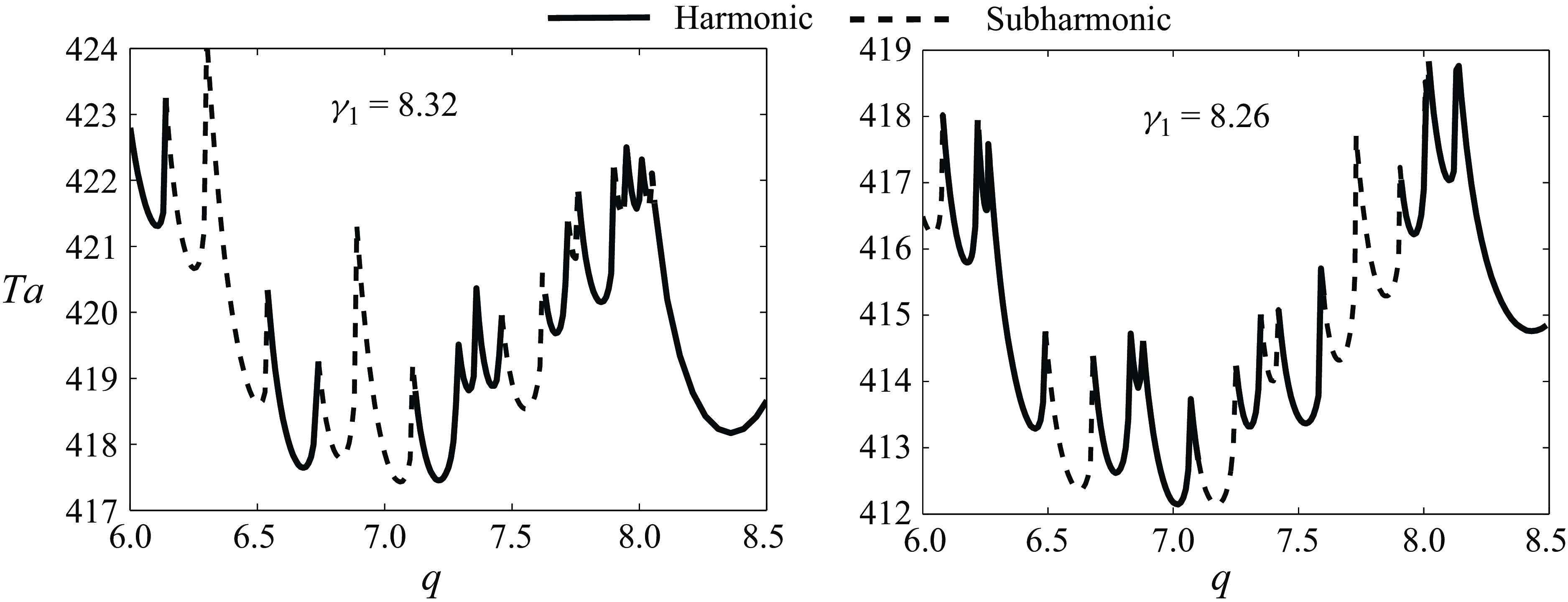
Such roughness is a signature of strong mode competition between different and numerous harmonic and subharmonic modes appearing in very narrow wavenumber ranges. To clearly elucidate this feature, two examples of marginal stability curves are depicted in figure 4 for two subsequent codimension-two bifurcation points detected at
 $\gamma _1 = 8.32$
and
 $\gamma _1 = 8.26$
. The first codimension-two bifurcation point is observed by crossing
 $\gamma _1 = 8.32$
and
 $\mathit{Ta}_c = 417.444$
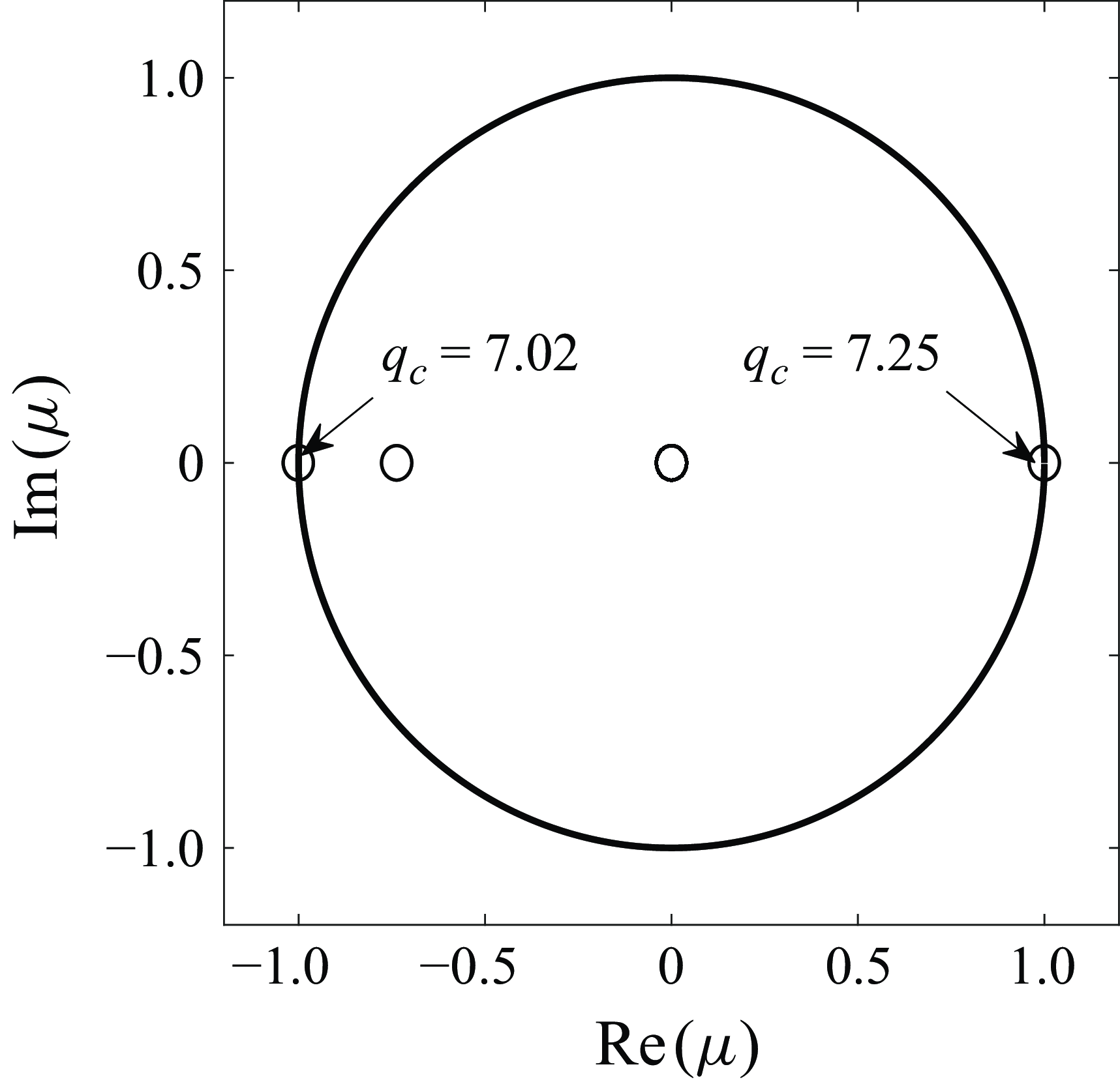
, where the system loses stability via two instability modes bifurcating simultaneously from the basic state at two critical wavenumbers, i.e
 $q_c = 7.02$
and
 $q_c = 7.25$
for the subharmonic (period-doubling) and (synchronous) harmonic modes, respectively. This feature is well illustrated in figure 5, that shows the calculated Floquet multipliers in the complex plane at the first codimension-two bifurcation point.
Marginal stability curves computed using Floquet theory showing two bicritical states between harmonic and subharmonic responses in the case where
 $\omega = 1/\sqrt {37}$
at
 $\gamma _1 = 8.32$
and
 $\gamma _1 = 8.26$
. On each curve, the vertical axis is the Taylor number
 $\mathit{Ta}$
while the horizontal one is the dimensionless axial wavenumber
 $q$
, ranging from 6 to 8.5.

Floquet multipliers at the bicritical state between harmonic and subharmonic instability modes reached at
 $\mathit{Ta}_c = 417.444$
,
 $q_c = 7.02$
,
 $q_c = 7.25$
when
 $\omega = 1/\sqrt {37}$
and
 $\gamma _1 = 8.32$
.

4.2. Burster identification strategy
Among the key characteristics of bursting behaviour is the slow and fast dynamics where the solution evolves slowly in some regions and suddenly jumps to a fast oscillatory state. This could be also observed from the phase portrait characterised by loops and clusters, i.e. a repetitive pattern where the system alternates between quiescent and oscillatory states.
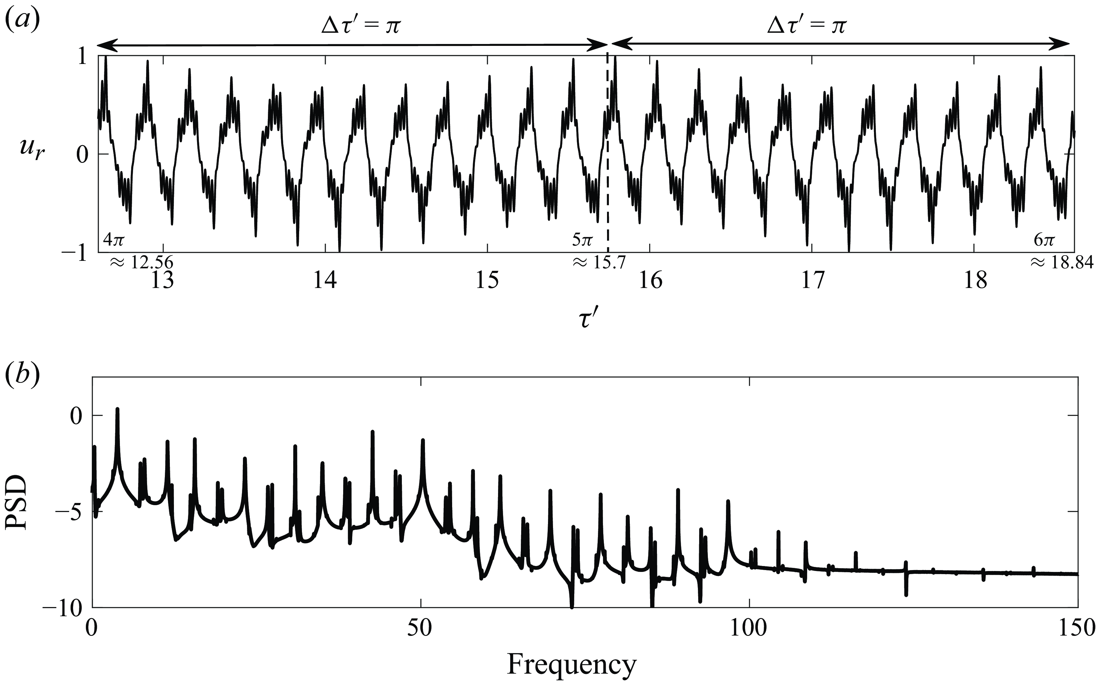
(a) Time series of the radial perturbation velocity and (b) its corresponding PSD recorded at the point
 $(x, \theta , z) = (1/2, 0, 0)$
over
 $2$
oscillation periods (
 $\tau ' \in [4T, 6T]$
) in the case where
 $\omega = 1/\sqrt {37}$
,
 $\gamma _1 = 10$
. The critical instability parameters are
 $\mathit{Ta}_c = 584.66$
and
 $q_c = 6.1$
.

In order to confirm the bursting nature of the left-hand axisymmetric instability mode observed in the marginal stability curve at the sufficiently high frequency
 $\gamma _1 = 10$
(figure 3), time series of the radial velocity and its corresponding power spectral density (PSD) at the point
 $(x, \theta , z) = (1/2, 0, 0)$
over
 $2$
oscillation periods (
 $\Delta \tau ' = 2\pi$
) are plotted in figure 6. It is evident that this time series is
 $\pi \hbox{-}$
periodic and exhibits a change of sign between negative and positive values. This behaviour means that we are dealing with a harmonic reversing flow characterised by sharp peaks, indicating fast oscillations superimposed on a slower modulation. There is no clear alternation between quiescent (low-amplitude) phases and sudden bursts as in classical bursting systems. However, the waveform suggests the presence of eigenmode interactions leading to sharp spikes. The PSD indicates that we are not dealing with a purely
 $\pi $
-periodic response, owing to the strong presence of additional frequency components. Also, the existence of sharp peaks suggests that the system is likely undergoing modulated periodic motion rather than fully chaotic bursting.
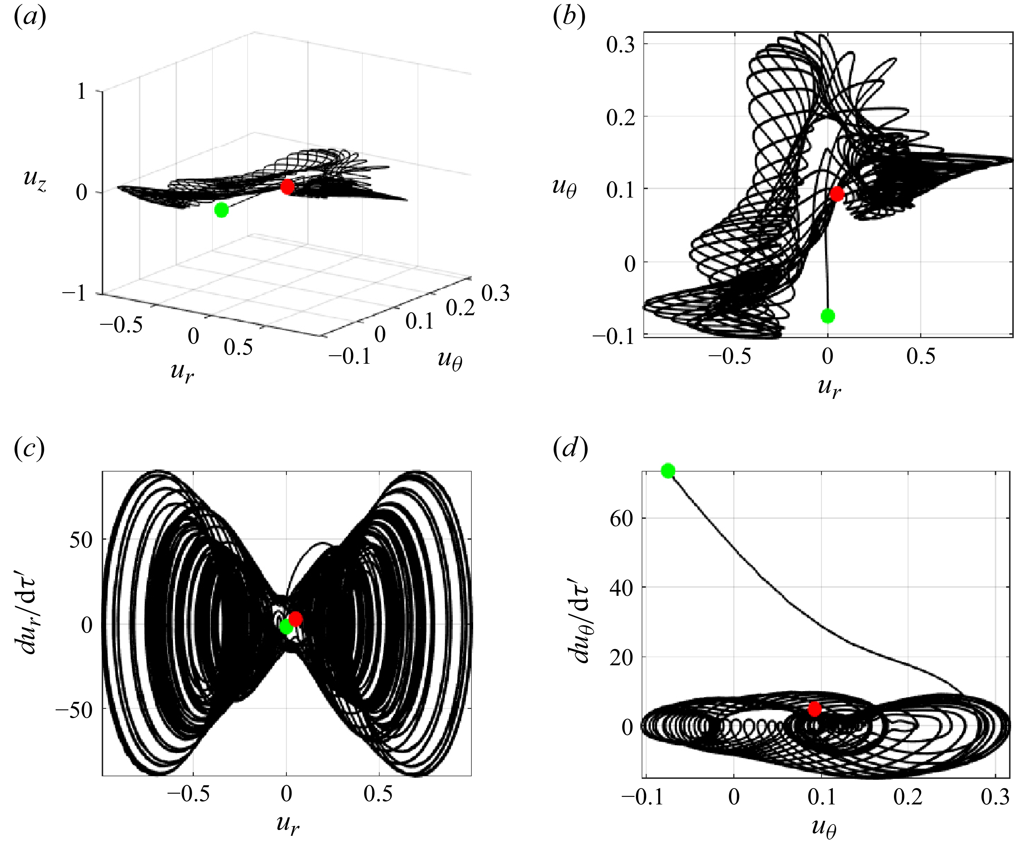
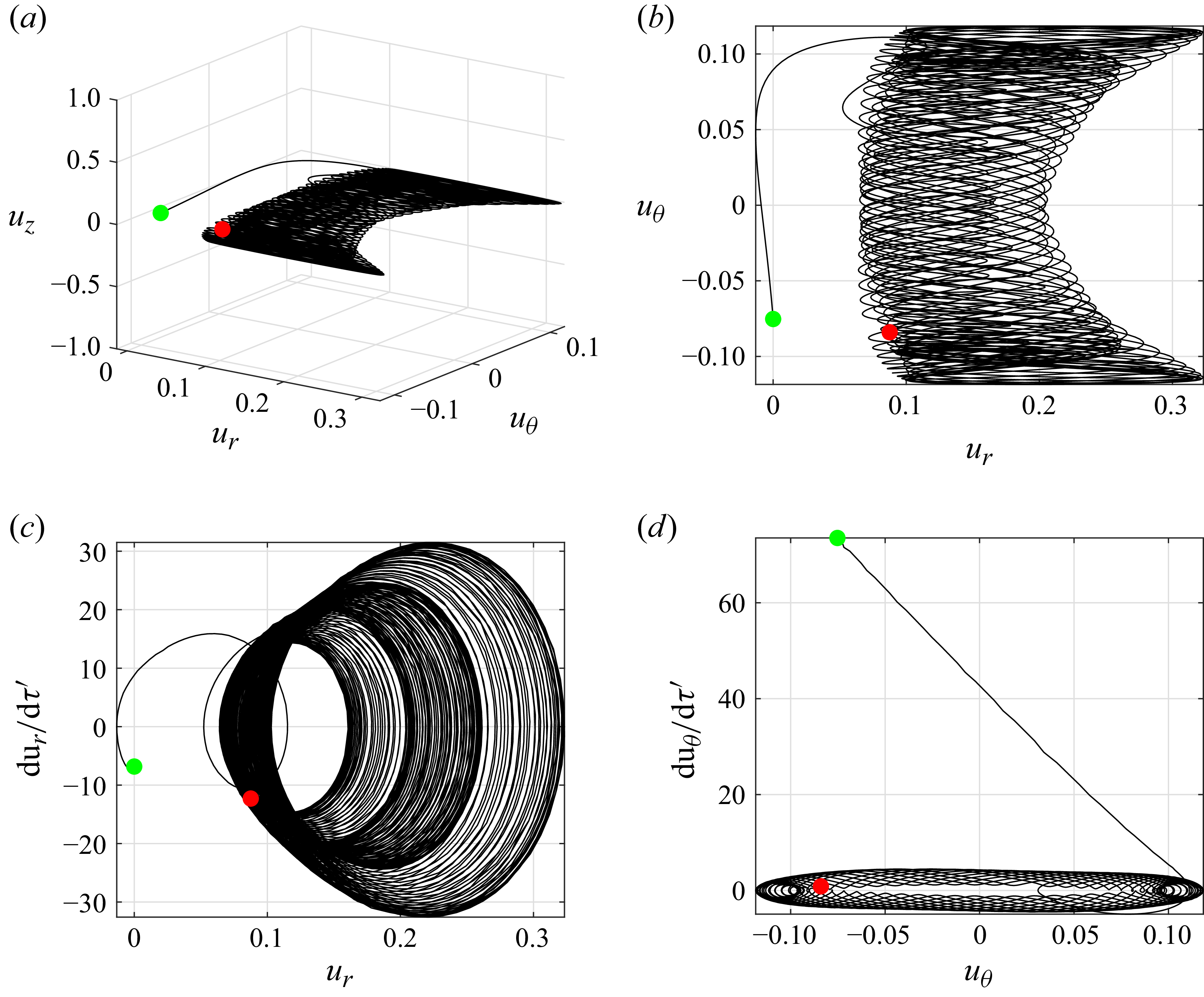
A set of phase portraits providing more insights into this instability mode is depicted in figure 7. Figure 7(a) represents a three-dimensional phase space using the
 $(u_r, u_\theta , u_z)$
velocities where it is noticed that the trajectory evolves in a confined, structured manner and exhibits oscillatory behaviour with slow and fast dynamics, a hallmark of bursting instabilities. Projection in the
 $(u_r, u_\theta )$
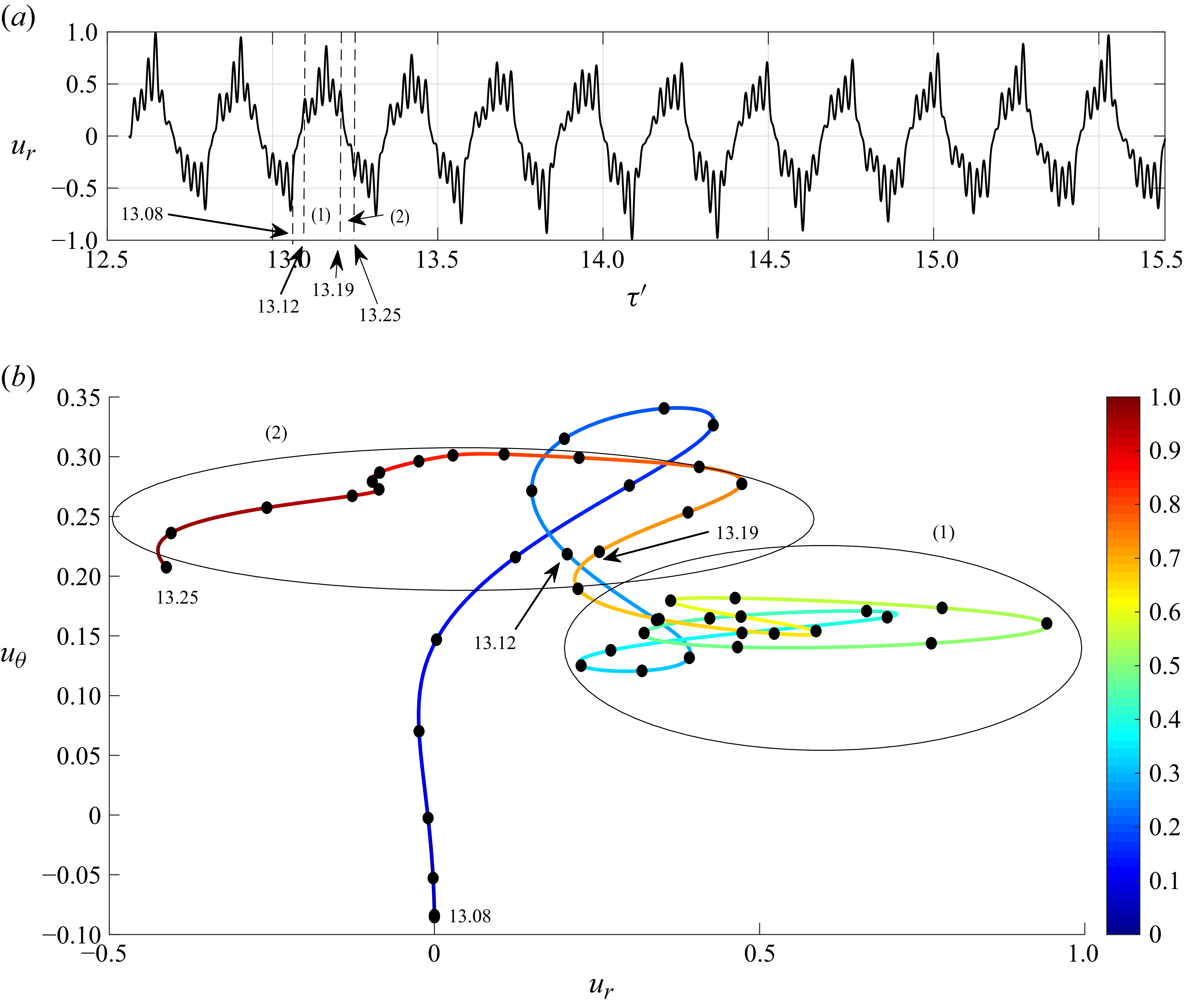
phase space is depicted in figure 7(b), which highlights the complex nature of the trajectory, suggesting a slow evolution around one region, followed by a rapid excursion (for a detailed version of this trajectory coloured by time along with time markers, readers should refer to figure 8). This is typical in slow–fast systems, reinforcing the idea of a bursting mode. A projection in the phase space
 $ (u_r, ( {{\rm d} u_r}/{{\rm d}\tau '}) )$
is illustrated in figure 7(c) showing a butterfly-shaped structure describing thus a classical bursting phase portrait. The latter sheds light on the trajectory that expands and contracts, forming two large lobes on both sides of
 $u_r = 0$
. Near this point, i.e.
 $u_r = 0$
, there are dense, chaotic-like oscillations, indicating a metastable state. This suggests that the system spends some time in a relatively slow phase before a burst occurs. In addition, this phase portrait shows fast excursions to large amplitudes where the system abruptly jumps to large values of
 $ {{\rm d} u_r}/{{\rm d}\tau '}$
, indicating thus the strong presence of rapid bursting events. These are characteristics of a slow–fast dynamics, where the system alternates between slow motion and rapid jumps (bursts). The projected trajectory in the
 $ (u_\theta , ( {{\rm d} u_\theta}/{{\rm d}\tau '}))$
space (figure 7
d) aligns with these conclusions and shows a rapid transition from a low-amplitude regime to a high-amplitude one.
Phase portraits illustrating the bursting instability mode obtained at the mid-gap
 $(x, \theta , z) = (1/2, 0, 0)$
when
 $\omega = 1/\sqrt {37}$
,
 $\gamma _1 = 10$
,
 $\mathit{Ta}_c = 584.66$
and
 $q_c = 6.1$
during the time interval
 $\tau ' \in [4T, 5T]$
. (a) Three-dimensional trajectory in the
 $(u_r, u_\theta , u_z)$
space, highlighting the oscillatory dynamics. (b) Projection onto the
 $(u_r, u_\theta )$
plane, showing the complex interplay between the radial and azimuthal velocity components. (c) Phase portrait in the
 $(u_r, ({{\rm d}u_r}/{{\rm d}\tau '}))$
space, revealing characteristic slow–fast transitions indicative of bursting behaviour. (d) Projection onto the
 $(u_\theta , ( {{\rm d}u_\theta }/{{\rm d}\tau '}))$
space, emphasising the role of azimuthal velocity variations. Parameters as in figure 6. The red and green markers represent respectively the final and initial instants.

(a) Time series of the radial perturbation velocity recorded at the point
 $(x, \theta , z) = (1/2, 0, 0)$
over one oscillation period (
 $\tau ' \in [4T, 5T]$
). (b) Time-coloured projection of the phase-space trajectory with equidistant time markers, highlighting the fast (sparser) and slow (denser) dynamics consistent with the temporal signal during the time interval
 $\tau ' \in [13.08, 13.25]$
. Parameters as in figure 6. The denser region (region 1) of the trajectory corresponds to slow evolution where the system remains temporarily trapped in an oscillatory regime in contrast to the sparser region (region 2) that reflects a fast transition between two oscillatory states as indicated by the steep slope in the time series signal.

From a physical point of view, bursting modes occur when interactions between two oscillatory Stokes layer flows generated near each cylinder are strongly involved (Riahi et al. Reference Riahi, Hayani Choujaa and Aniss2025). It is interesting to recall here that, at these frequencies, i.e.
 $\gamma _1 = 10$
and
 $\gamma _2 = \gamma _1/\sqrt {\sqrt {37}} \approx 0.405\gamma _1 \approx 4.05$
, a purely oscillatory Stokes layer flow sets in near the inner cylinder, meaning that this oscillatory flow generates a damped viscous wave whose penetration depth does not exceed the Stokes layer thickness
 $\delta _1 = 0.1d$
. Meanwhile, the penetration depth of the damped viscous wave generated by the outer cylinder, i.e.
 $\delta _2 = 2.46d$
, is greater than
 $\delta _1$
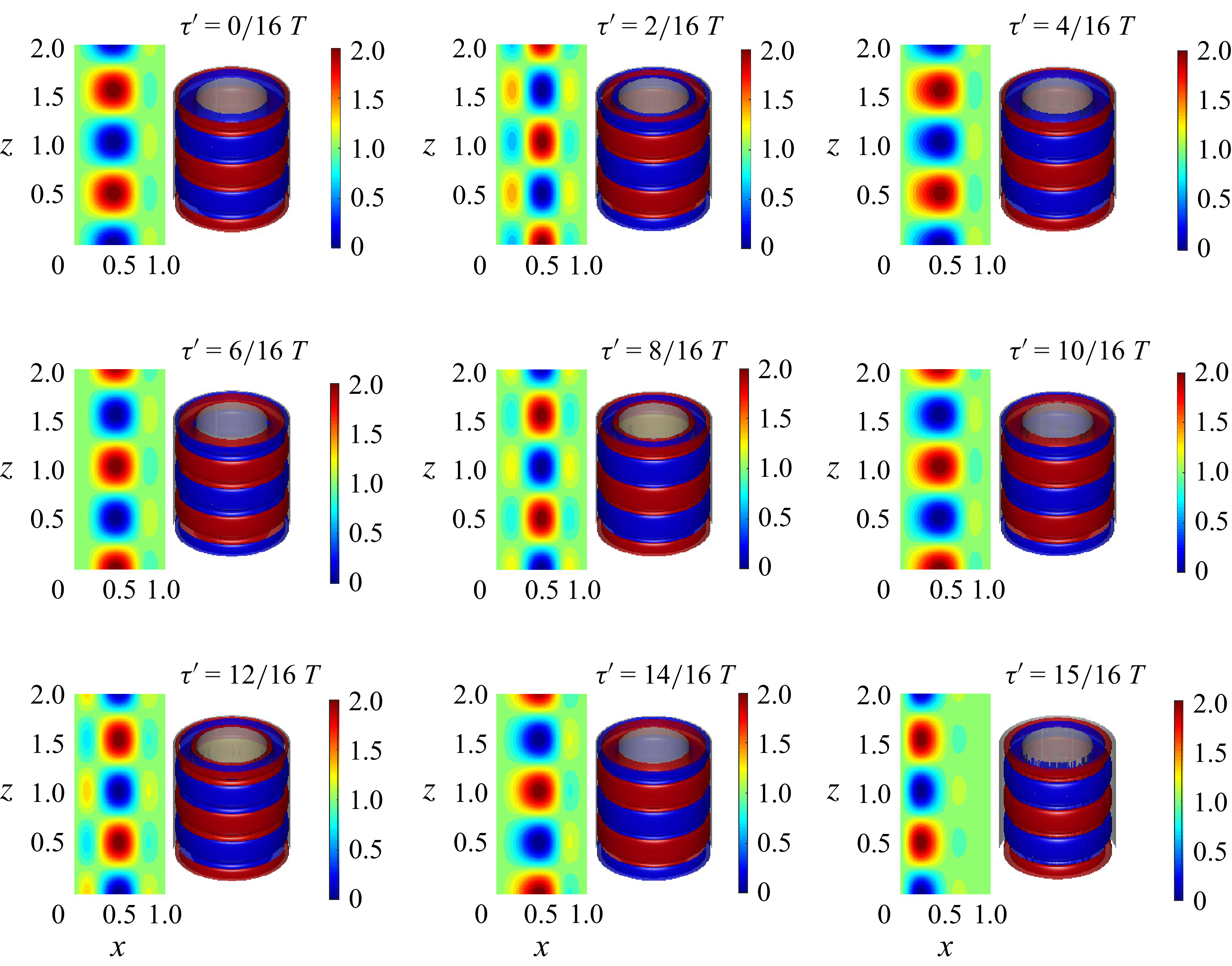
and requires more than the gap width to be attenuated. This feature suggests that we are dealing with a flow configuration mainly controlled by the outer cylinder drive. The veracity of these speculations is substantiated and clearly illustrated in snapshots of two-dimensional (2-D) and 3-D contour plots of the radial component of the perturbed velocity field depicted in figure 9 over one oscillation period. As one can see, the gap between the cylinders is filled by pairs of large Taylor vortices rotating in a privileged direction (clockwise say for vortices located at a representative vertical position, e.g.
 $z = 0.5$
) at
 $\tau ' = 0$
with small vortices, having opposite polarity (anti-clockwise say at
 $z = 0.5$
), near the outer cylinder. These small outer-cylinder-driven vortices undergo a growth process over time and transport, towards the inner cylinder, the large vortices that become smaller at
 $\tau ' = T/8$
. Other outer-cylinder-driven vortices, rotating in the clockwise direction, emerge and become larger just after
 $\tau ' = T/8$
, suppressing thus the existing vortices. This scenario is repeated several times during one period and highlights the reversing flow process in this parameter space. The burster is generated by interactions, taking place near the inner cylinder, between the rapid and repetitive small outer-cylinder-driven vortices and the inner cylinder drive. The latter pushes these vortices inwards (see the instants
 $\tau ' = 15/16T$
and
 $\tau ' = 4/16T$
) or outwards depending on the instantaneous order of magnitude of the drives.
Snapshots of the radial component of the perturbed velocity field relative to the bursting instability mode using two visualisation modes. The left panel displays a 2-D contour plot, while the right panel presents a 3-D isosurface rendering. These snapshots have been taken after transients have vanished. In particular, a time shift of four periods
 $t \to t - 4T$
is applied. Parameters as in figure 6.

It is interesting to note here that this bursting mode exists at
 $\gamma _1 = 10$
but it is considered as the primary bifurcation of the system just within the frequency interval
 $8.35 \prec \gamma _1 \prec 8.75$
where the Stokes layer thicknesses
 $\delta _1$
and
 $\delta _2$
become larger, enhancing thus the bursting phenomenon. The strong contribution of the outer cylinder drive is evident in this bursting mode in contrast to the most unstable mode observed at this frequency, i.e.
 $\gamma _1 = 10$
, where the Taylor vortex flow becomes mainly driven by the inner cylinder. At
 $\gamma _1 = 10$
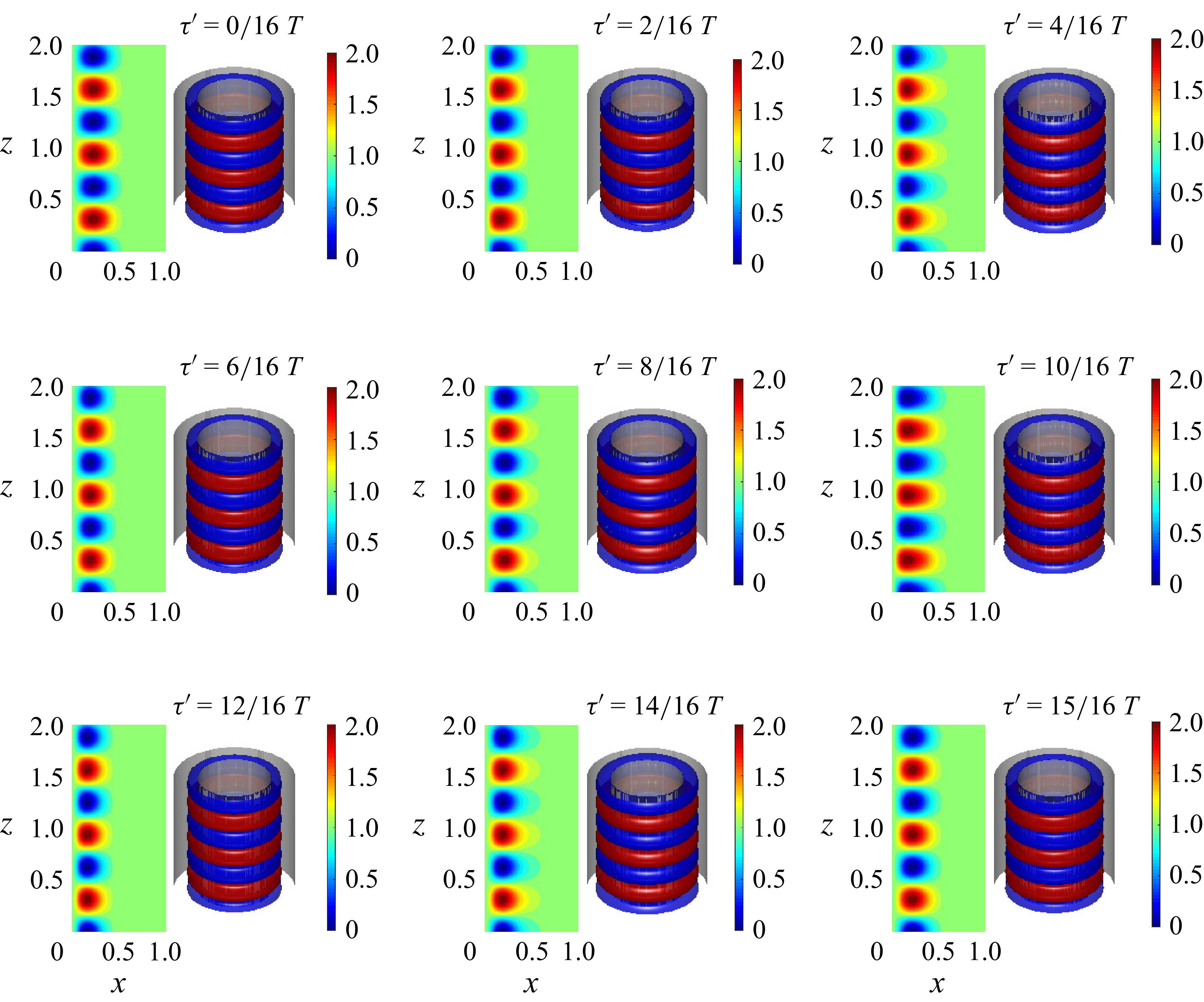
, the resulting flow corresponds to a regular oscillatory Stokes layer flow adjacent to the inner cylinder, as is well depicted in figure 10 using the same snapshots as in figure 9. This means that no interactions between the Stokes layer flows generated by the cylinders are expected when dealing with regular instability modes.
Phase portraits equivalent to those used in figure 7 are illustrated in figure 11 and are related to the regular instability mode observed at
 $\gamma _1 = 10$
. These phase portraits suggest a different type of dynamic behaviour compared with the previous bursting one. Indeed, this figure shows more structured, layered oscillations, especially in panels (a) and (b), which might indicate transitions between different periodic states. In panel (c), it is evident that we are dealing with a superposition of numerous and different limit cycles characterised by different frequencies. This behaviour aligns quite well with the multi-frequencies observed in the PSD of the time series of the local radial velocity, illustrated by Riahi et al. (Reference Riahi, Hayani Choujaa and Aniss2025) for this instability mode in this parameter space.
Snapshots of the radial component of the perturbed velocity field relative to the regular instability mode using two visualisation modes. The left panel displays a 2-D contour plot, while the right panel presents a 3-D isosurface rendering. These snapshots have been taken after transients have vanished at
 $\omega = 1/\sqrt {37}$
,
 $\gamma _1 = 10$
,
 $\mathit{Ta}_c = 511.8685$
and
 $q_c = 10.3$
. In particular, a time shift of four periods
 $t \to t - 4T$
is applied.

Phase portraits illustrating the regular instability mode obtained at the mid-gap
 $(x, \theta , z) = (1/2, 0, 0)$
when
 $\omega = 1/\sqrt {37}$
,
 $\gamma _1 = 10$
,
 $\mathit{Ta}_c = 511.8685$
and
 $q_c = 10.3$
during the time interval
 $\tau ' \in [4T, 5T]$
. Panels are similar to those used in figure 7.

4.3. Bursters at different approached values of the frequency ratio
 $\omega$
: the case
$\omega = \sqrt {3}$


A strong relationship exists between the computational costs of the numerical calculations and the approached values assigned to the frequency ratio parameter
 $\omega$
in the sense that, the higher the integers values of
 $\tilde {p}$
and
 $\tilde {q}$
in the stability problem, the longer calculation time required. The subsequent investigation seeks to ascertain the impact of the designated values for the integer parameters
 $\tilde {p}$
and
 $\tilde {q}$
on both the critical instability parameters and the burster phenomenon. That is to say, what are the lowest values of
 $\tilde {p}$
and
 $\tilde {q}$
for which the critical instability parameters and the burster phenomenon remain unaffected?
The frequency ratio
 $\omega = \sqrt {3}$
, for instance, can be approached by different ratios. If one considers the decimal number
 $7/4 = 1.75$
where
 $\tilde {p} = 7$
and
 $\tilde {q} = 4$
as an underestimated value of
 $\sqrt {3} \approx 1.73205$
with an absolute error of
 $0.01795$
, we are dealing with a periodic forcing system whose quasiperiodic character is not involved. This is not the case if one approaches the number
 $\sqrt {3}$
by the rational number
 $26/15 \approx 1.73333\ldots$
, where
 $\tilde {p} = 26$
and
 $\tilde {q} = 15$
, or by
 $97/56 \approx 1,7321428\ldots$
, where
 $\tilde {p} = 97$
and
 $\tilde {q} = 56$
. In these cases, the quasiperiodicity is strongly involved.
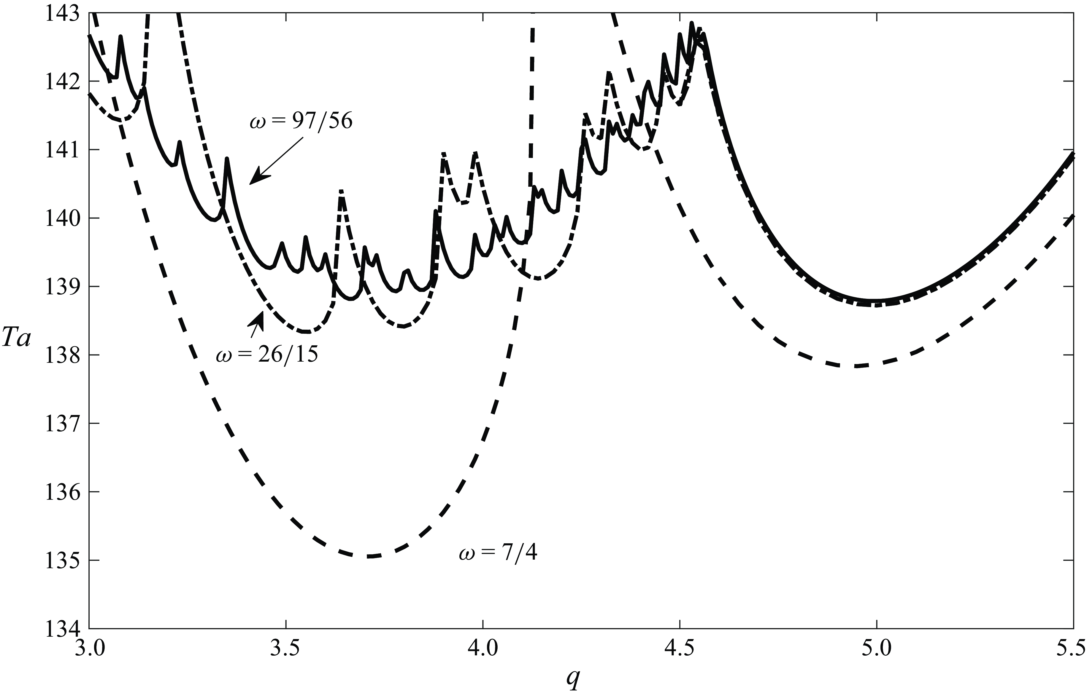
Figure 12 illustrates marginal stability curves when different approached values are assigned to the frequency ratio
 $\omega = \sqrt {3}$
when
 $\gamma _1 = 3.155$
. We consider especially the ratios
 $7/4, 26/15$
and
 $97/56$
. As one can notice, when
 $\omega = 7/4$
, only two smooth instability branches, corresponding to two regular modes, are observed, meaning that no bursting modes occur in this case. However, the left-hand stability branch becomes rough when
 $\omega = 26/15$
, indicating the existence of numerous instability modes, a hallmark of the bursting phenomenon. Such bursting becomes more pronounced and intense when
 $\omega = 97/56$
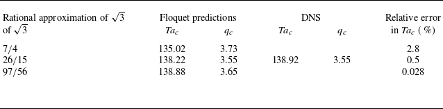
while the critical instability parameters remain almost unchanged. This feature means that the bursting phenomenon is a consequence of the non-periodic character in the forcing system that injects two different time scales into the stability problem. It is also interesting to point out that the critical instability parameters are weakly dependent on the nature of the approached value to the frequency ratio such as
 $\mathit{Ta}_c = 135.02$
at
 $q_c = 3.73$
at
 $\omega = 7/4$
,
 $\mathit{Ta}_c = 138.22$
at
 $q_c = 3.55$
at
 $\omega = 26/15$
against
 $\mathit{Ta}_c = 138.8$
at
 $q_c = 3.65$
at
 $\omega = 97/56$
. This means that approaching
 $\sqrt {3}$
by
 $362/209$
or
 $1351/780$
leads to a great increase in both the computational cost and the number of the stability modes constituting the rough branch in the stability curve in contrast to the critical instability parameters that remain unchanged.
By comparing these critical instability parameters with the benchmark values obtained by direct numerical simulations (performed recently by Riahi et al. Reference Riahi, Hayani Choujaa and Aniss2025) where the ratio
 $\sqrt {3}$
is fully taken into account, one can conclude that the Floquet predictions, based on rational approximations of
 $\sqrt {3}$
, exhibit rapid convergence toward the direct numerical simulation (DNS) results. The relative error between Floquet and DNS computations falls below 0.5
 $\,\%$
for ratios higher than 7/4, confirming thus the accuracy and reliability of the rational-approximation method (see table 1 for more details).
Comparison between Floquet predictions obtained using different rational approximations of the irrational frequency ratio
 $\omega = \sqrt {3}$
and DNS results adopted by Riahi, Hayani Choujaa and Aniss (Reference Riahi, Hayani Choujaa and Aniss2025). The relative error is defined as
 $|\mathit{Ta}_c^{(\textit{Floquet})} - \mathit{Ta}_c^{(\textit{DNS})}|/\mathit{Ta}_c^{(\textit{DNS})}$
.

By limiting the frequency number
 $\sqrt {3}$
to the first number after the decimal point
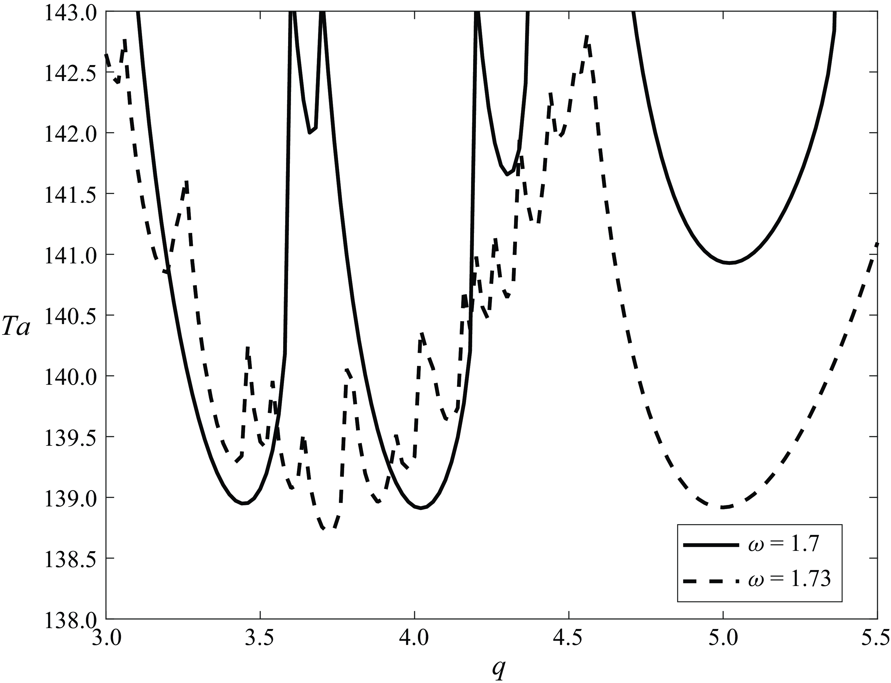
 $\sqrt {3} \approx 1.7$
, which is equivalent to the decimal ratio number
 $17/10$
, only four instability modes are detected in the marginal stability curve computed at the same frequency
 $\gamma _1 = 3.155$
, as depicted in figure 13. However, by considering
 $\sqrt {3} \approx 1.73\,(173/100)$
we reproduce quite well the same marginal stability curve obtained at
 $\sqrt {3} \approx 97/56$
but the required calculation time becomes significantly larger.
Marginal stability curves computed using Floquet theory at
 $\gamma _1 = 3.155$
when the frequency
 $\omega = \sqrt {3}$
is approached by different ratios:
 $\omega \approx 7/4$
,
 $\omega \approx 26/15$
and
 $\omega \approx 97/56$
. The vertical axis is the Taylor number
 $\mathit{Ta}$
while the horizontal one is the dimensionless axial wavenumber
 $q$
, ranging from 3 to 5.5.

Marginal stability curves computed using Floquet theory at
 $\gamma _1 = 3.155$
when the frequency
 $\omega = \sqrt {3}$
is approached by different rational ratios:
 $\omega \approx 1.7$
and
 $\omega \approx 1.73$
. The vertical axis is the Taylor number
 $\mathit{Ta}$
while the horizontal one is the dimensionless axial wavenumber
 $q$
, ranging from 3 to 5.5.

4.4. Effect of the quasiperiodic frequency ratio
$\omega$
on the stability diagrams of axisymmetric disturbances

4.4.1. The case
$\omega \succ 1$
:
$\omega = \sqrt {3}$


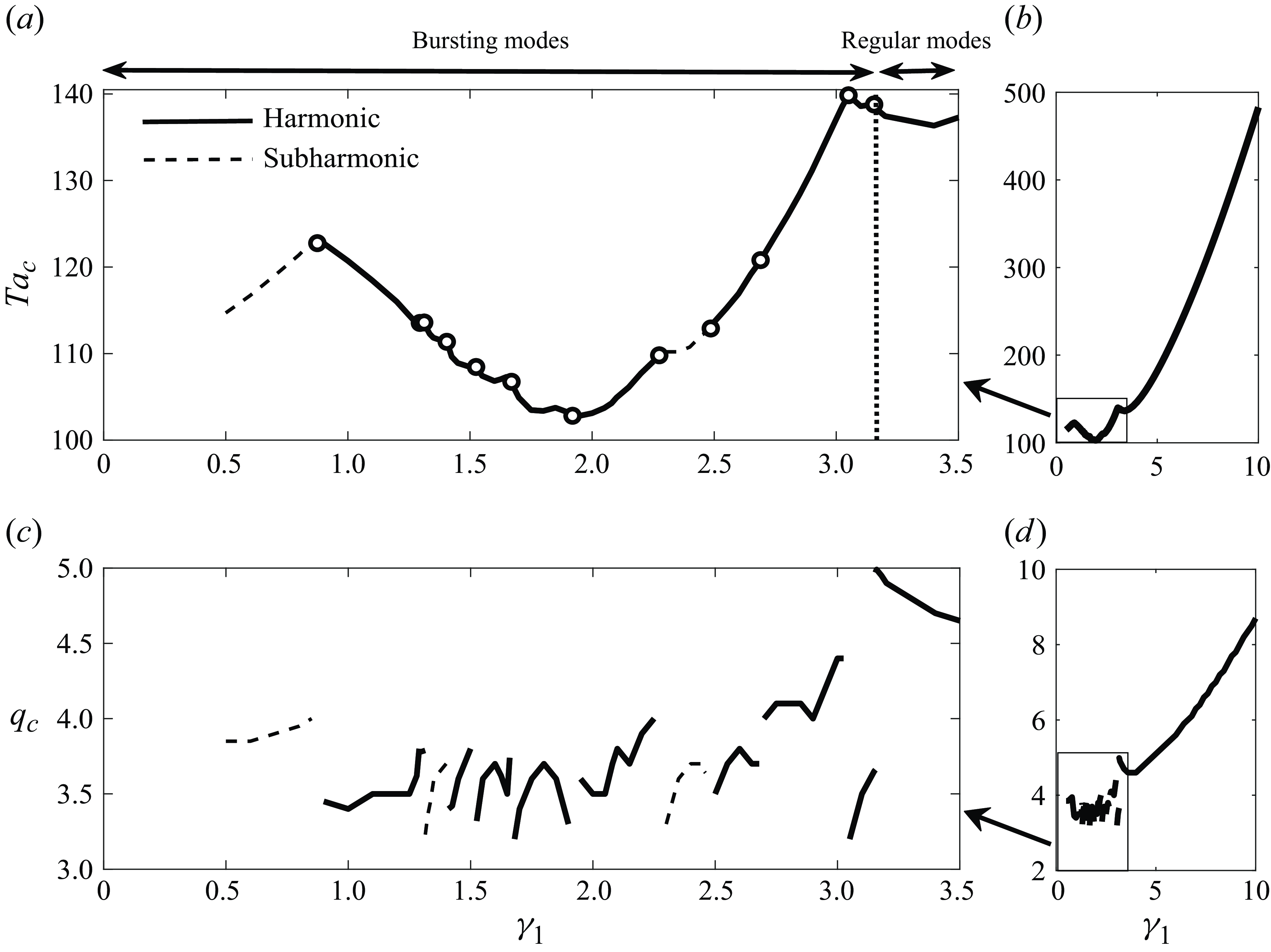
Stability diagrams obtained by Floquet analysis in the case where
 $\omega = \sqrt {3}$
. Panels show (a, b)
 $\mathit{Ta}_c(\gamma _1)$
and (c, d)
 $q_c(\gamma _1)$
.

By considering axisymmetric disturbances, i.e.
 $m = 0$
, we illustrate in figure 14 a stability diagram showing the evolution of the critical Taylor number (figure 14
a,b) and wavenumber (figure 14
c,d) versus the inner cylinder oscillation frequency when the quasiperiodic frequency parameter
 $\omega = \sqrt {3}$
is approached by
 $97/56$
. Due to the strong presence of numerous instability modes, we plot these critical instability parameters in figure 14(a,c) in the frequency intervals
 $\gamma _1 \in [0, 3.5]$
and in figure 14(b,d) when
 $\gamma _1 \in [0, 10]$
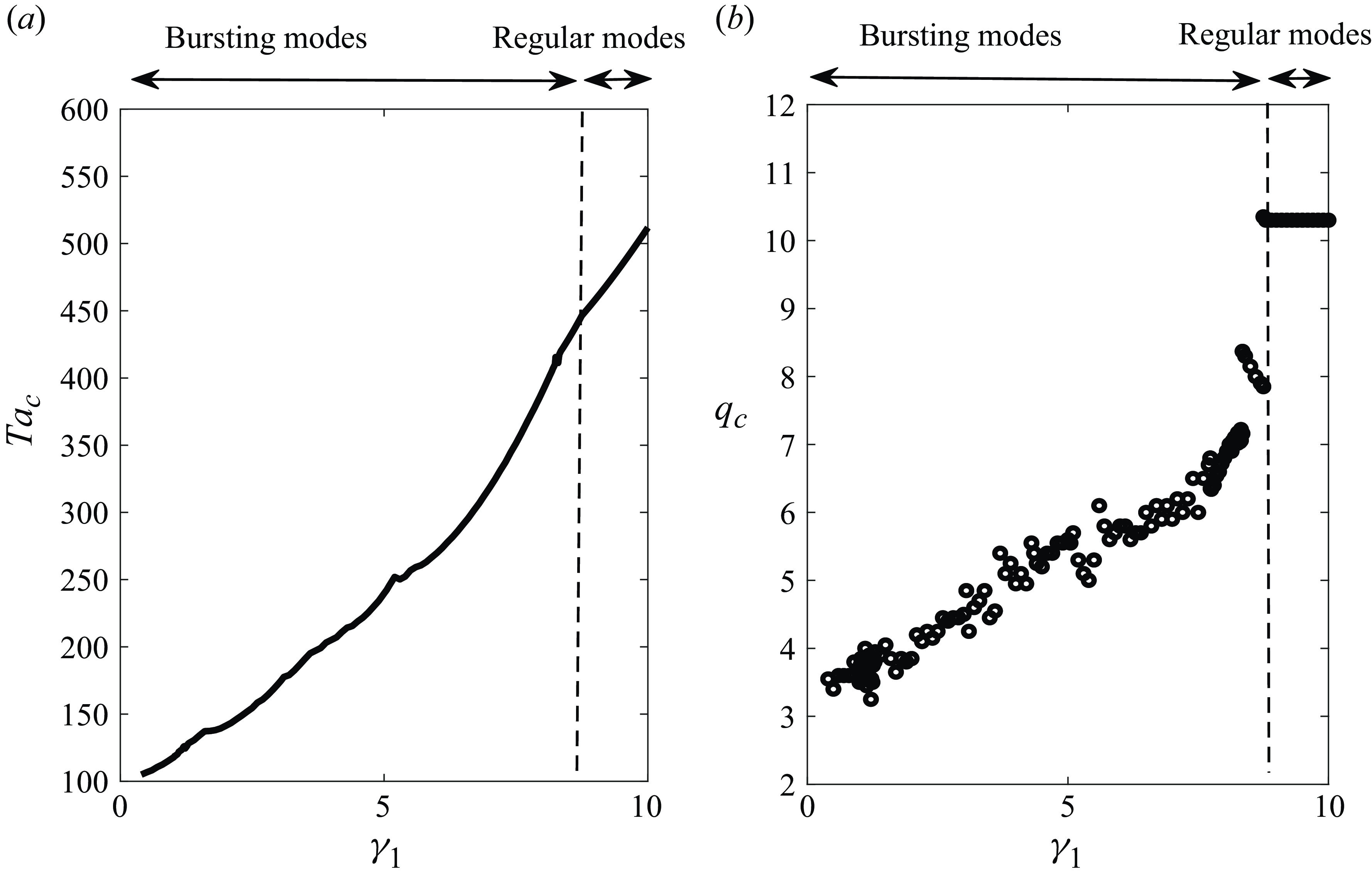
. As one can see, these stability diagrams are composed of thirteen branches, resulting in twelve cusp points/discontinuities in the critical Taylor/wavenumber curve. This feature is due to the multiplicity of the flow states emerging under the effect of the irrational frequency number
 $\omega$
. The instability exchange between these states occurs via codimension-two bifurcation points, giving rise to twelve bicritical states in the computed marginal stability curves. This bicriticality sets in between either two harmonic, two subharmonic instability modes, or harmonic and subharmonic instability modes. For instance, the first bicritical state between two harmonic modes occurs at
 $\gamma _1 = 3.155$
, where a drop in
 $q_c$
from
 $5$
to
 $3.65$
is detected. This means that, at this frequency, two harmonic Taylor vortex flows with different critical wavenumbers bifurcate simultaneously from the laminar basic state. The flow reversal nature of these modes could be identified on the basis of time series of the local radial velocity of the disturbances whose change of sign indicates opposite polarity of the Taylor vortices. Recently, Riahi et al. (Reference Riahi, Hayani Choujaa and Aniss2025) have demonstrated that at
 $\gamma _1 = 10$
we are dealing with a regular non-reversing flow whereas at
 $\gamma _1 = 3.1$
a bursting reversing flow emerges. This means that the quasiperiodic nature of the frequency ratio alters the flow reversal of the system where non-reversing/reversing flows set in within the frequency interval
 $\gamma _1 \succ 3.2/ \gamma _1 \prec 3.2$
when
 $\omega = \sqrt {3}$
against
 $\gamma _1 \succ 1.3/\gamma _1 \prec 1.3$
when
 $\omega = 1$
(Riahi et al. Reference Riahi, Aniss and Ouazzani Touhami2019).
The second bicritical state occurs between two harmonic reversing flows at
 $\gamma _1 = 2.9$
, where a drop in
 $q_c$
from
 $4.5$
to
 $3.1$
is detected, while others are observed between harmonic and subharmonic modes at
 $\gamma _1 = 2.5, 2.3, 1.45, 1.27, 0.78$
. It is important to mention here that subharmonic instability modes do not appear when
 $\omega = 1$
and this is one of the important features induced by the presence of a two-frequency forcing.
In addition, one should highlight the flow stabilisation observed in the high-frequency limit where the critical Taylor number reproduces quite well the asymptotic behaviour obtained in the case
 $\omega = 1$
where:
 $\mathit{Ta}_c = 15.28\gamma ^{3/2}$
(Aouidef et al. Reference Aouidef, Normand, Stegner and Wesfreid1994; Riahi et al. Reference Riahi, Aniss and Ouazzani Touhami2019). Nevertheless, the low-frequency behaviour of the system is significantly altered by the presence of the quasiperiodicity
 $\omega$
. Indeed, the overall trend of the system is towards more destabilisation, especially when
 $\gamma _1 \prec 0.8$
, instead of a stabilisation in the same frequency range when
 $\omega = 1$
. This feature means that when
 $\omega = \sqrt {3}$
, the system is no longer potentially unstable at an intermediate-frequency value and therefore the frequencies
 $\gamma _{1p}$
and
 $\gamma _{2p}$
lose their physical relevance in the current context.
To understand this behaviour, one can recall the low-frequency behaviours of the system under different boundary conditions. Indeed, when the outer cylinder is slowly oscillating and the inner one is fixed, Riahi, Hayani Choujaa & Aniss (Reference Riahi, Hayani Choujaa and Aniss2024) have demonstrated using Floquet theory and two quasi-steady approaches that the system remains linearly stable, similarly to the steady rotation case of the cylinder. This result is in agreement with those obtained by Carmi & Tustaniwskyi (Reference Carmi and Tustaniwskyj1981). This means that the oscillation of the outer cylinder alone does not lead to any kind of instability, in contrast to the case where the only oscillating cylinder is the inner one, where the system loses stability at
 $\mathit{Ta}_c = 41.31$
and
 $q_c \to 3.12$
(Krueger et al. Reference Krueger, Gross and Di Prima1966; Riahi et al. Reference Riahi, Aniss, Ouazzani Touhami and Skali Lami2015) similarly to the steady rotation case. However, when both the inner and outer cylinders are slowly co-oscillating with the same frequency, the system becomes equivalent to a solid body rotation or to inviscid fluid flow where the shear strain between the cylinders vanishes and consequently
 $\mathit{Ta}_c$
tends towards infinity (
 $\mathit{Ta}_c \to \infty$
) (Aouidef et al. Reference Aouidef, Normand, Stegner and Wesfreid1994; Riahi et al. Reference Riahi, Aniss and Ouazzani Touhami2019). When the cylinders are slowly oscillating with two incommensurate frequencies, two irrational time scales are involved and a phase lag between the flows generated by each cylinder is created. A shear strain between the cylinders is then produced and the dynamics of the system becomes governed by the inner cylinder forcing, especially when the outer cylinder forcing does not lead to flow destabilisation, as demonstrated in Carmi & Tustaniwskyi (Reference Carmi and Tustaniwskyj1981), Riahi et al. (Reference Riahi, Hayani Choujaa and Aniss2024). In this framework, the low-frequency behaviour
 $\mathit{Ta}_c = 41.31$
and
 $q_c \to 3.12$
could be expected. This question will be discussed and studied in detail in § 5, where a quasi-steady analysis assuming low-frequency oscillations of the cylinders with an incommensurate frequency ratio is performed.
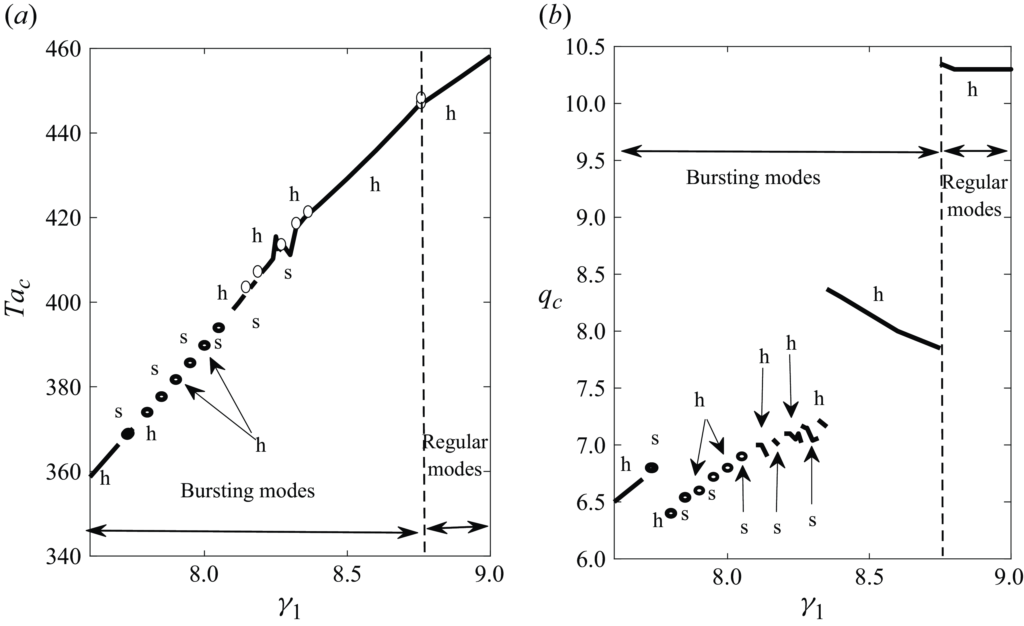
Stability diagram obtained by Floquet theory over the frequency interval
 $\gamma _1 \in [7.6, 9]$
in the case where
 $\omega = 1/\sqrt {37}$
: (a)
 $\mathit{Ta}_c(\gamma _1)$
and (b)
 $q_c(\gamma _1)$
. Here, ‘s’ and ‘h’ denote subharmonic and harmonic modes, respectively.

4.4.2. The case
$\omega \lt 1$
:
$\omega = 1/ \sqrt {37}$


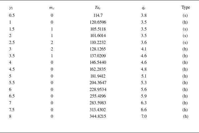
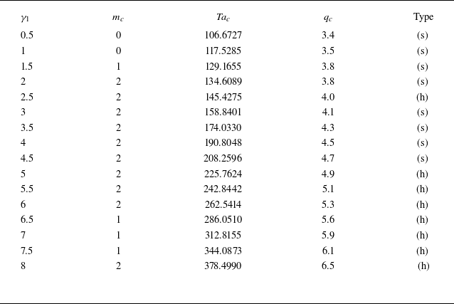
In figure 15, stability diagrams related to the case
 $\omega = 1/ \sqrt {37}$
when it is approached by
 $12/73$
are depicted for
 $\gamma _1 \in [7.6, 9]$
. As one can notice, the frequency range when the regular modes (non-reversing) set in shrinks, i.e.
 $\gamma _1 \succ 8.75$
in contrast to
 $\gamma _1 \succ 3.155$
when
 $\omega = \sqrt {3}$
. This means that, in comparison with the case
 $\omega = \sqrt {3}$
, the bursting frequency range becomes larger where we are dealing with a complex behaviour owing to the strong interplay between families of harmonic and subharmonic modes (reversing). Consequently, this stability diagram is composed of several instability branches featuring several codimension-two bifurcation points besides discontinuities in the critical wavenumber and cusp points in the Taylor number evolution, as shown in figure 16. With a decrease in the frequency
 $\gamma _1$
, the overall trend is towards destabilisation, similarly to the case
 $\omega = \sqrt {3}$
. In the low-frequency limit, one can envisage a constant critical Taylor number and wavenumber close to those calculated for a fixed outer cylinders, i.e.
 $\mathit{Ta}_c \to 41.31$
and
 $q_c \to 3.12$
(Krueger et al. Reference Krueger, Gross and Di Prima1966; Riahi et al. Reference Riahi, Aniss, Ouazzani Touhami and Skali Lami2015).
It is worth noting that a small frequency step is required, in this case, in order to capture all the eventually involved instability modes whose nature is very sensitive to the frequency number
 $\gamma _1$
.
The strong mode competition renders the experimental reproduction of the present results difficult. Pattern formation and abrupt changes in the critical wavenumber that may be obviously determined experimentally from the spatial structure of the Taylor cells could, however, be used as an efficient tool to distinguish between different primary instability modes arising when the frequency parameter
 $\gamma _1$
changes.
It is important to point out that the uncovered burster phenomenon in this study is a consequence of applying two incommensurate frequencies to the inner and outer drives of a Taylor–Couette system. These bursts are linked to resonance phenomena that could be induced or suppressed via an appropriate choice of input frequencies. Such behaviour has numerous real-world practical implications ranging from energy-efficient flow control and enhanced mixing to signal-based modulation in rotating systems. The dependence of bursting on the frequency forcing ratios suggests efficient strategies for regulating flow states in applications where hydrodynamic instabilities are undesired due to geometric constraints or high energy costs. By a proper tuning of the incommensurate frequency ratio, one can operate at regular, weakly and strongly bursting regimes and effectively the flow intensity or mixing characteristics are controlled without changing system geometry or fluid properties.
Stability diagram obtained by Floquet theory over the frequency interval
 $\gamma _1 \in [0, 10]$
in the case where
 $\omega = 1/\sqrt {37}$
: (a)
 $\mathit{Ta}_c(\gamma _1)$
and (b)
 $q_c(\gamma _1)$
.

4.5. Effect of the quasiperiodic frequency ratio
$\omega$
on the axisymmetric stability diagrams

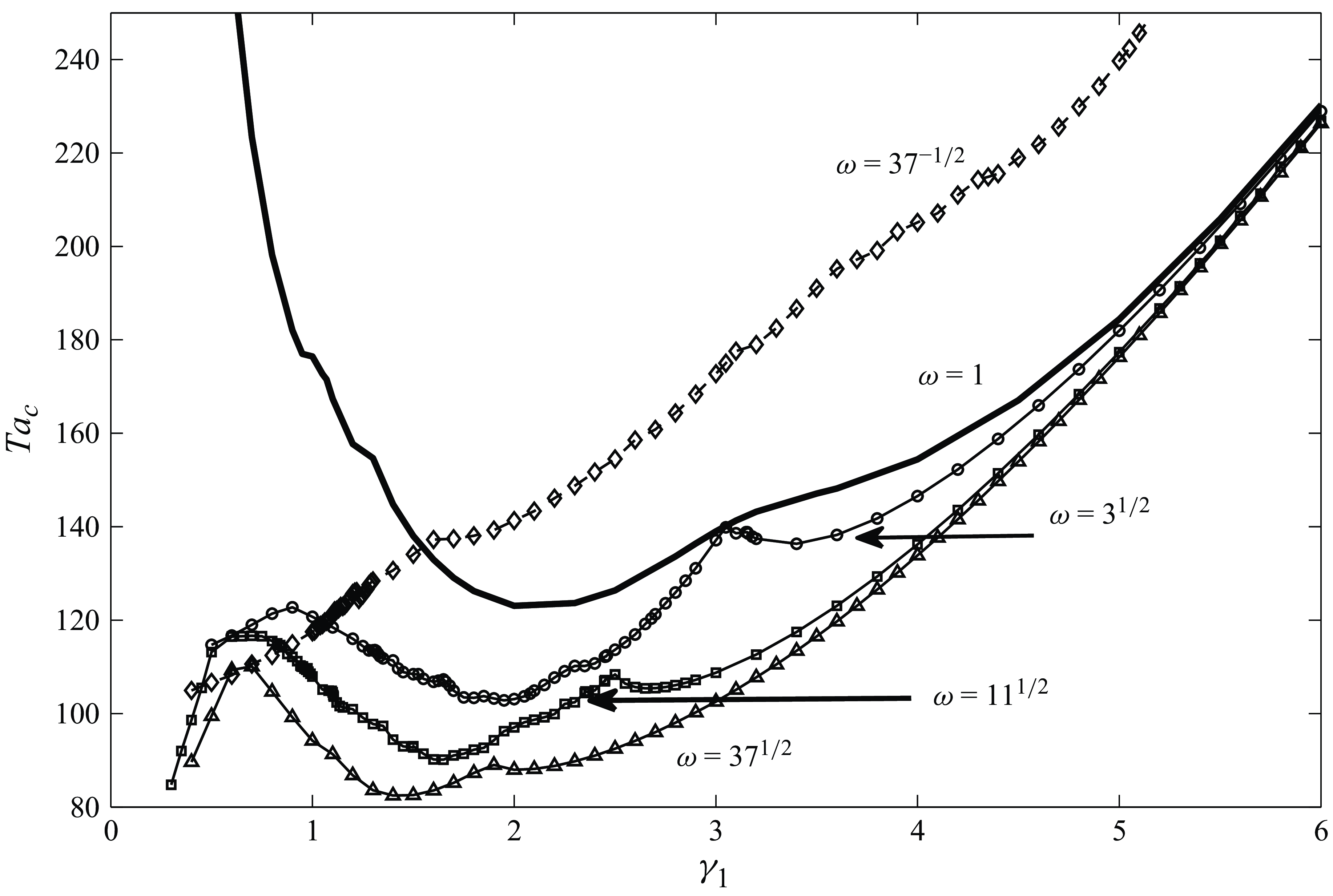
In figure 17, we report stability diagrams computed at different values of the quasiperiodic frequency ratio in order to shed light on the effect of this latter on the onset of axisymmetric instabilities. This feature will be better elucidated by comparing the results related to the case
 $\omega \neq 1$
with those for
 $\omega = 1$
. It is important to mention here that two other values of
 $\omega$
are considered, namely
 $\omega = \sqrt {37}$
and
 $\omega = \sqrt {11}$
when they are approached respectively by
 $37/12$
and
 $63/19$
. As one can see, the quasiperiodic frequency parameter
 $\omega$
does not alter the stability of the system when the frequency of the cylinders is sufficiently high provided that
 $\omega \succ 1$
(
 $\omega _2 \succ \omega _1$
). In this case, we are dealing with an unstable oscillatory Stokes layer flow occurring especially in narrow regions near the inner cylinder. Therefore, the critical Taylor number in this frequency range is reminiscent of that obtained for the case of an oscillating inner cylinder with a fixed outer one and the cases of co- and counter-oscillating cylinders with
 $\omega = 1$
(Riahi et al. Reference Riahi, Aniss and Ouazzani Touhami2019, Reference Riahi, Hayani-Choujaa and Aniss2022):
 $\mathit{Ta}_c = 15.28 \gamma _1^{3/2}$
.
Stability diagrams obtained by Floquet analysis for different values of the parameter
 $\omega$
.

The bifurcated solutions in this high-frequency limit correspond to regular non-reversing Taylor vortex flows that emerge when
 $\gamma _1 \succ 3.85$
for
 $\omega = \sqrt {1.1}$
,
 $\gamma _1 \succ 3.7$
for
 $\omega = \sqrt {1.2}$
,
 $\gamma _1 \succ 3.155$
for
 $\omega = \sqrt {3}$
,
 $\gamma _1 \succ 2.4$
for
 $\omega = \sqrt {11}$
,
 $\gamma _1 \succ 1.85$
for
 $\omega = \sqrt {37}$
and
 $\gamma _1 \succ 1.3$
for
 $\omega = 1$
. Therefore, one can conclude that the irrationality of the frequency ratio enhances/inhibits the reversing/non-reversing Taylor vortex flow. In comparison with the case
 $\omega = 1$
, the quasiperiodic frequency ratio in this case has a destabilising effect, which becomes more pronounced in the low-frequency limit. The parameter
 $\omega$
does not considerably alter the critical Taylor number in this frequency limit, where it is expected that the oscillating inner cylinder becomes the main destabilising drive of the system.
Particular behaviour is observed in the case
 $\omega \prec 1$
, i.e.
 $\omega _1 \succ \omega _2$
, especially at
 $\omega = 1/\sqrt {37}$
where non-reversing solutions emerge only when
 $\gamma _1 \succ 8.75$
. In this case, and in comparison with the case
 $\omega = 1$
, the quasiperiodic parameter ratio
 $\omega$
has a stabilising effect which becomes less pronounced by decreasing the frequency
 $\omega _1$
. A cross-over point is reached at
 $\gamma _1 \approx 1.5$
below which the effect of
 $\omega$
becomes destabilising. In the low-frequency limit, the critical Taylor number becomes close to the critical values calculated when
 $\omega \succ 1$
.
In previous studies dealing with time-quasiperiodic forcing, Boulal et al. (Reference Boulal, Aniss, Belhaq and Rand2007, Reference Boulal, Aniss, Belhaq and Azouani2008) and Boulal et al. (Reference Boulal, Riahi and Aniss2024), who were interested in studying the effect of quasiperiodic gravitational modulation on the stability of a heated fluid layer, have shown that the quasiperiodic frequency
 $\omega$
alters the stability characteristics of the system if it belongs to the interval
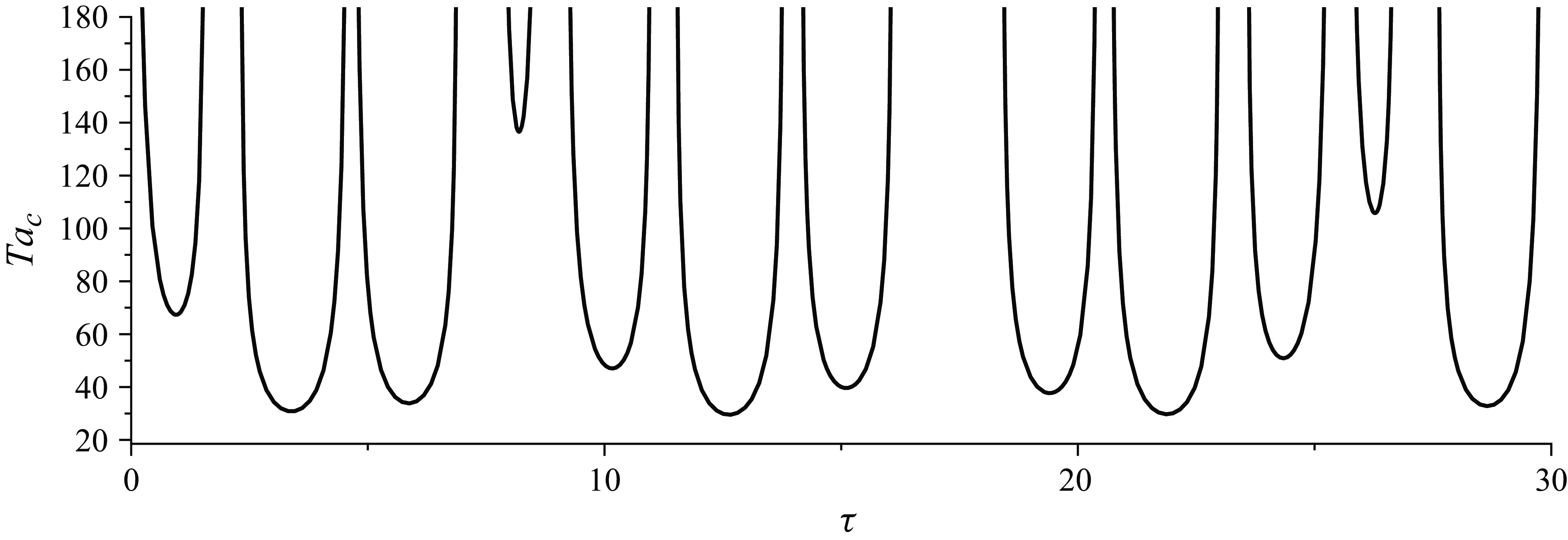
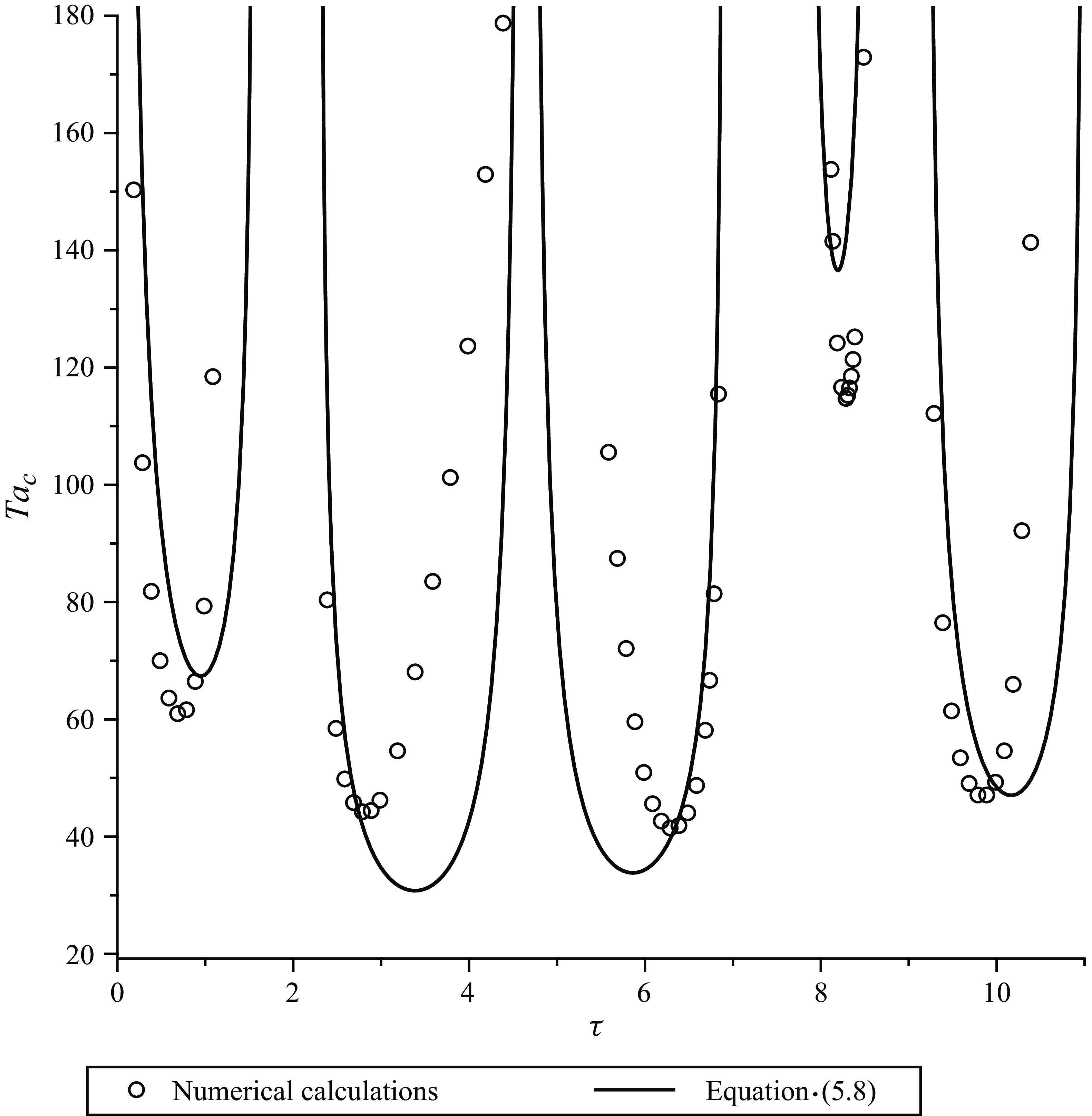
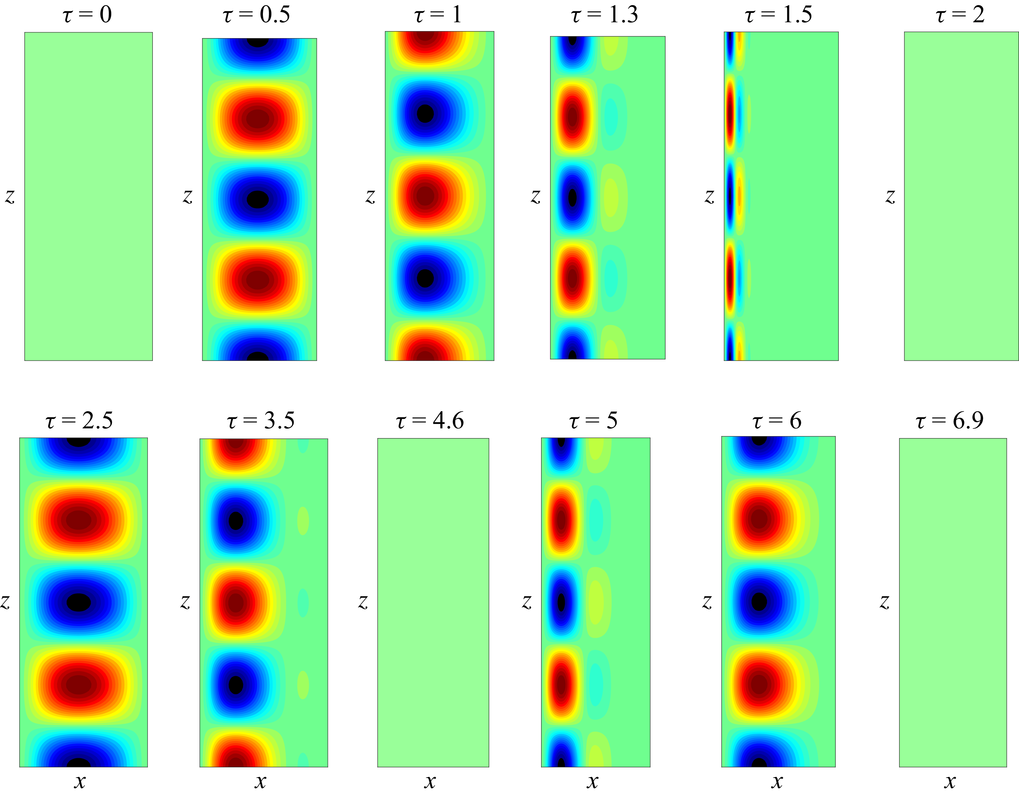
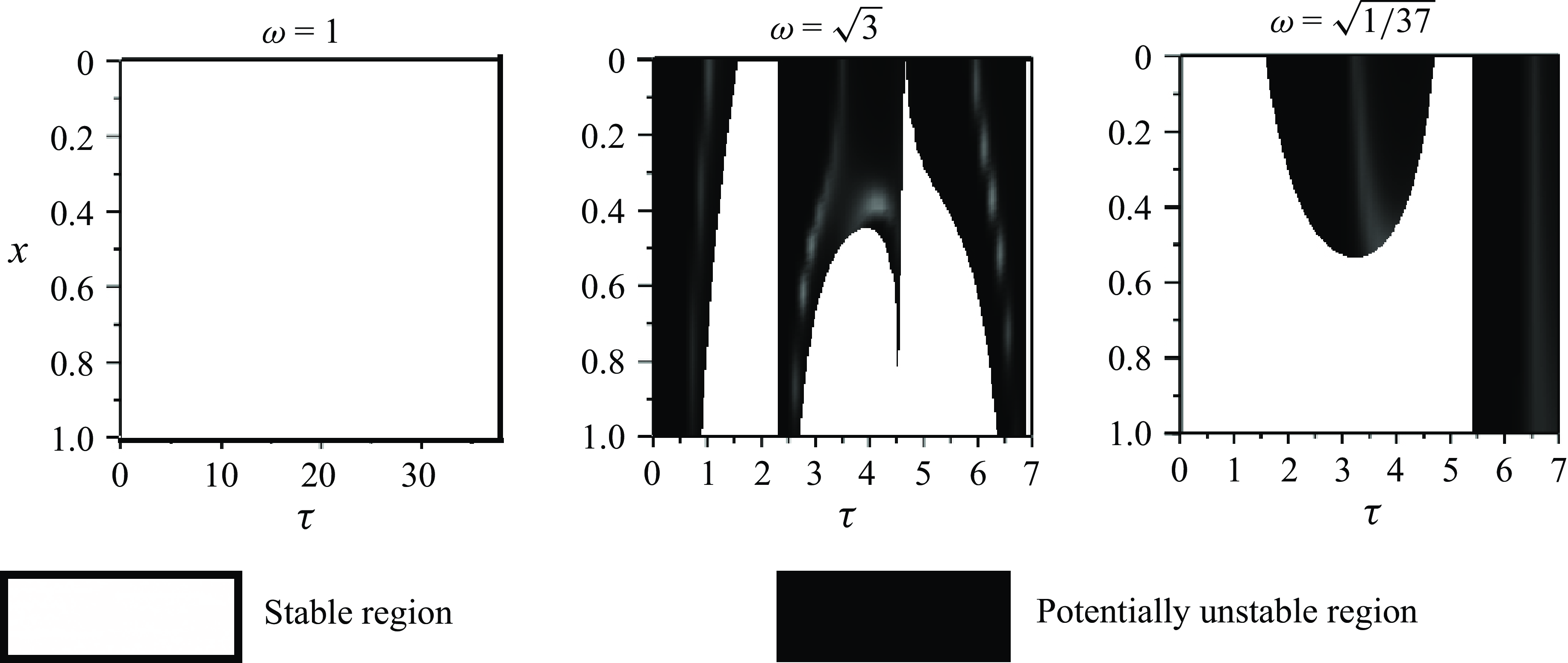
 $(( {1}/{\sqrt {37}}), \sqrt {37})$
. Similar behaviour has been observed by Yagoubi & Aniss (Reference Yagoubi and Aniss2017), who studied the effect of vertical quasiperiodic vibrations on the Faraday instability. When dealing with time-quasiperiodically modulated Taylor–Couette flow, this feature is conserved only when
 $\gamma _1 \succcurlyeq 1.5$
.
4.6. Effect of the quasiperiodic frequency ratio
$\omega$
on the primary bifurcation taking into account non-axisymmetric disturbances

In this subsection, we shed light on the ability of the quasiperiodic frequency ratio
 $\omega$
in changing the axisymmetric nature of the primary bifurcation with respect to the case
 $\omega = 1$
studied experimentally by Aouidef et al. (Reference Aouidef, Normand, Stegner and Wesfreid1994). This purpose can be reached by a numerical resolution of the stability equations under small and continuous variations of the wavenumber
 $k$
. The resulting marginal stability curves, showing evolution of the Taylor number versus the axial wavenumber, allow the identification of the most unstable mode. The latter is three-dimensional and non-axisymmetric if the critical Taylor number calculated at
 $k = 0$
is higher than that at
 $k \neq 0$
. The critical value of the wavenumber
 $k$
, denoted
 $k_c$
, corresponds to that of the lowest value of the critical Taylor number. In such cases, the critical azimuthal wavenumber is calculated from the relation
 $k_c = m_c \varepsilon ^{1/2}$
for a given value of
 $\varepsilon \ll 1$
, where only positive integer values of
 $m_c$
are physically significant. This procedure requires a wide enough range of real values of
 $k$
to accurately identify the nature of the most unstable mode and determine its critical wavenumber
 $m_c$
. However, one can achieve the same objective in a simpler manner by choosing a definite value of
 $\varepsilon$
and numerically resolving the stability equations when only integer values are assigned to the azimuthal wavenumber
 $m$
. In the present paper,
 $\varepsilon = 0.14$
is adopted in our numerical calculations since it is a reasonable small-gap value in typical experimental geometries. We recall here that Feugaing et al. (Reference Feugaing, Crumeyrolle, Yang and Mutabazi2014) carried out experiments for
 $\varepsilon = 0.139$
in the case where the outer cylinder is fixed while the inner one is rotating with an angular velocity modulated in time about a non-zero mean value. At sufficiently small modulation amplitudes, their experimental instability parameters are in excellent agreement with the classical ones calculated using the narrow-gap approximation (Chandrasekhar Reference Chandrasekhar1961). Experimental results obtained by Aouidef et al. (Reference Aouidef, Normand, Stegner and Wesfreid1994) with
 $\varepsilon = 0.11$
reproduce quite well their numerical findings in the co-oscillating case with
 $\omega = 1$
using the narrow-gap approximation. Due to the rich and complex dynamics observed at
 $m = 0$
and owing to the wide frequency range considered in this study, our attention is restricted only to some values of the frequency
 $\gamma _1$
.
For
 $\omega = \sqrt {3}$
, we found that the most unstable mode is no longer axisymmetric, especially at the frequencies
 $\gamma _1 = 1.5$
,
 $\gamma _1 = 2$
and
 $\gamma _1 = 3.5$
where
 $m_c = 1$
and
 $\gamma _1 = 2.5$
and at
 $\gamma _1 = 3$
where
 $m_c = 2$
. These results are presented in table 2. It is also important to mention that the quasiperiodic parameter alters also the type of the most unstable mode where non-axisymmetric subharmonic responses set in at some frequencies, e.g.
 $\gamma _1 = 2$
, where the axisymmetric modes are harmonic.
Numerical values of the critical instability parameters, i.e.
 $(\mathit{Ta}_c, q_c, m_c)$
, at different values of the frequency
 $\gamma _1$
when the quasiperiodic frequency parameter
 $\omega = \sqrt 3$
.

The same dynamics is observed when
 $\omega = 1/\sqrt {37}$
, as shown in table 3. One can mention in this case that non-axisymmetric instability modes are more suitable than axisymmetric modes.
Numerical values of the critical instability parameters, i.e.
 $(\mathit{Ta}_c, q_c, m_c)$
, at different values of the frequency
 $\gamma _1$
when the quasiperiodic frequency parameter
 $\omega = 1/\sqrt {37}$
.

5. Low-frequency behaviour: quasi-steady analysis and Rayleigh discriminant
5.1. Local quasi-steady analysis
In this section, a quasi-steady analysis is conducted to understand the low-frequency behaviour of the system, depicted in the stability diagrams in figure 17, obtained using Floquet theory for axisymmetric disturbances. The main purpose is to validate our speculations concerning the contributions of the inner and outer cylinders in the Taylor vortices formation.
In this framework, the time derivatives are neglected from the stability equations and a numerical resolution of the obtained equations is performed at given values of time which appear only as a parameter in the basic flow expression. This analysis has been widely used in the literature to investigate the low-frequency behaviour of hydrodynamical systems subjected to time-periodic forcing (Aouidef et al. Reference Aouidef, Normand, Stegner and Wesfreid1994; Aouidef & Normand Reference Aouidef and Normand1996, Reference Aouidef and Normand2000; Ern Reference Ern1998; Ern & Wesfreid Reference Ern and Wesfreid1999, Reference Ern and Wesfreid2002; Luo & Wu Reference Luo and Wu2010; Riahi et al. Reference Riahi, Aniss, Ouazzani Touhami and Skali Lami2014, Reference Riahi, Aniss, Ouazzani Touhami and Skali Lami2015, Reference Riahi, Aniss, Ouazzani Touhami and Skali Lami2016; Riahi et al. Reference Riahi, Aniss and Ouazzani Touhami2019). This analysis reproduces quite well experimental findings in a variety of time-modulated Taylor–Couette flows with different boundary conditions. When the cylinders are co-oscillating about zero mean with two superimposed frequencies, Ern & Wesfreid (Reference Ern and Wesfreid2002) showed experimentally, by ultrasound Doppler velocimetry, the existence of a spike-like behaviour in the amplitude of the axial flow with several successive growths, dampings and periods of quietness. Their numerical calculations performed using the same quasi-steady analysis revealed the same behaviour in terms of the critical Taylor number where several stable and unstable regions emerge depending on the forcing time history.
By considering
 $\tau = \omega _1 t$
,
 $\omega _1 \ll 1$
and
 $\omega _2 \ll 1$
, the asymptotic expression of the basic state and its
 $x$
-derivative at the leading order are written as
 \begin{eqnarray} V_{\!B}(x, \tau ) &=& (1-x) \cos (\tau ) + x \cos (\omega \tau ) +h.o.t\,\,\,\mbox{and}\,\,\, \nonumber \\\textit{DV}_{\!B}(x, \tau ) &=& - \cos (\tau ) + \cos (\omega \tau ) + h.o.t., \end{eqnarray}
where
 $h.o.t.$
is the High order terms, while the stability equations related to axisymmetric disturbances are reduced, after neglecting the term
 $\omega _1 \partial /\partial \tau$
, to
 \begin{align} &\left (\frac {d^2}{{\rm d}x^2} - q^2 \right )^2 \hat {u}_r = 2 q^2 \mathit{Ta}^2 V_{\!B}(x, \tau ) \hat {u}_\theta , \end{align}
 \begin{align} &\left (\frac {d^2}{{\rm d}x^2} - q^2 \right ) \hat {u}_\theta = \frac {{\rm d} V_{\!B}(x, \tau )}{{\rm d} x}\hat {u}_r. \end{align}
To get a simplified form of these stability equations that could explain the behaviour of the system when the cylinders are oscillating with different frequencies, let us neglect the velocity expression produced by the oscillating outer cylinder, i.e.
 $x \cos (\omega \tau )$
, only from the function
 $V_{\!B}(x, \tau )$
and keep it at
 $\textit{DV}_{\!B}(x, \tau )$
. The obtained stability equations correspond to the classical Taylor–Couette system with a steadily rotating inner cylinder and a fixed outer one as follows:
 \begin{align} &\left (\frac {d^2}{{\rm d}x^2} - q^2 \right )^2 \hat {u'}_r = 2 q^2 \widetilde { \mathit{Ta}}^2 (1-x) \hat {u}_\theta , \end{align}
 \begin{align} &\left (\frac {d^2}{{\rm d}x^2} - q^2 \right ) \hat {u}_\theta = - \hat {u'}_r , \end{align}
where
 $\widetilde { \mathit{Ta}} = \mathit{Ta} \sqrt {\cos (\tau ) ( \cos (\tau ) - \cos (\omega \tau ) )}$
and
 $\hat {u'}_r = ( \cos (\tau ) - \cos (\omega \tau ) )\hat {u}_r$
with the boundary conditions
 \begin{equation} \hat {u'}_r=\hat {u}_\theta =\frac {\partial \hat {u'}_r}{\partial x}=0\,\,\,\,\,\,\mbox{at}\,\,\,x=0\,\,\,\,\mbox{and}\,\,\,\,x=1. \end{equation}
The well-known solution of the classical boundary value system (5.4)–(5.6) given in terms of the critical Taylor number and wavenumber is
 \begin{eqnarray} \widetilde { \mathit{Ta}}_c = 41.31\,\,\,\mbox{and}\,\,\,q_c = 3.12, \end{eqnarray}
giving rise to the following instability parameters:
 \begin{eqnarray} \mathit{Ta}_c = \dfrac {41.31}{\sqrt {\cos (\tau )\left ( \cos (\tau ) - \cos (\omega \tau )\right )}} \,\,\,\mbox{and}\,\,\,q_c = 3.12. \end{eqnarray}
Time evolution of the critical Taylor number given by (5.8) at
 $\omega = \sqrt {3}$
is illustrated in figure 18, where a spike-like behaviour is shown with several successive growths, dampings and periods of quietness. Such behaviour is reminiscent of that reported by Ern & Wesfreid (Reference Ern and Wesfreid2002) using both experimental measurements and the same numerical approach. Using the expression (5.8) one can explain the quietness times, also called ‘intermittent instability’, usually appearing in time-modulated Taylor–Couette systems driven by two time-dependent forcings with different frequencies (Ern & Wesfreid Reference Ern and Wesfreid2002). Indeed, these times of quietness are solutions of the inequality
 $\cos (\tau ) ( \cos (\tau ) - \cos (\omega \tau ) ) \preccurlyeq 0$
where the system is considered linearly stable, i.e. no critical values of the Taylor number exist. This means that if the inner cylinder is rotating in the clockwise direction (say), i.e.
 $\cos (\tau ) \preccurlyeq 0$
, the basic state is laminar as long as
 $\cos (\tau ) \succcurlyeq \cos (\omega \tau )$
, which correspond to times instants where the inner drive is higher than the outer one, i.e.
 $\varOmega _{\textit{in}} \succcurlyeq \varOmega _{\textit{out}}$
. However, when the inner cylinder reverses its direction of rotation, i.e.
 $\cos (\tau ) \succcurlyeq 0$
, the basic state is laminar as long as
 $\cos (\tau ) \preccurlyeq \cos (\omega \tau )$
, i.e.
 $\varOmega _{\textit{in}} \preccurlyeq \varOmega _{\textit{out}}$
.
The minimum value of
 $\mathit{Ta}_c$
is reached when the term
 $\sqrt {\cos (\tau ) ( \cos (\tau ) - \cos (\omega \tau ) )}$
reaches its maximum value, which corresponds to
 $1.4$
. This value is independent of the parameter
 $\omega$
. Consequently, the asymptotic behaviour of the critical Taylor number and wavenumber in the low-frequency limit does not depend on the quasiperiodic parameter ratio
 $\omega$
and is given by
 \begin{eqnarray} \mathit{Ta}_c = 29.71\,\,\,\mbox{and}\,\,\,q_c = 3.12. \end{eqnarray}
Time evolution of the critical Taylor number given by (5.8) at
 $\omega = \sqrt {3}$
.

To have a more accurate asymptotic behaviour related to these critical instability parameters, one should have recourse to a numerical resolution of the stability system (5.3) by taking into account all terms in the basic velocity expression (5.1) and its
 $x$
-derivative without any restrictions. Using the spectral method for a spatial discretisation of the system (5.3), as described in Appendix A, a system of
 $2N$
coupled ordinary differential equations is obtained and written as
 \begin{equation} \overline {\overline {\mathrm{A}}}\widehat {\mathrm{\boldsymbol {X}}}=\mathit{Ta}\,\overline {\overline {\mathrm{B}}}\widehat {\mathrm{\boldsymbol {X}}}, \end{equation}
where
 $\widehat {{\boldsymbol {X}}} = (\hat {u'}_{r_0}, \hat {u'}_{r_1}, \hat {u'}_{r_2},\ldots ,\hat {u'}_{r_N},\hat {u}_{\theta _0}, \hat {u}_{\theta _1}, \hat {u}_{\theta _2}, \ldots , \hat {u}_{\theta _N})^\textrm{T}$
and
 $\overline {\overline {\mathrm{A}}}$
and
 $\overline {\overline {\mathrm{B}}}$
are
 $2N\times 2N$
matrices. In this case,
 $\mathit{Ta}$
is the eigenvalue of the system which is solved at each instant to address a marginal stability curve whose minimal point coordinates represent the critical Taylor number and its corresponding wavenumber. Evolution of the instantaneous critical Taylor number is depicted in figure 19 at
 $\omega = \sqrt {3}$
. As one can notice, these numerical calculations reproduce the same behaviour as described by (5.8) and reported in figure 18. What should be noticed in terms of the differences is the sharpening of the spike-like behaviour and the increase in the critical Taylor number where
 $\mathit{Ta}_c = 41.262$
is detected at
 $\tau = 6.3$
with
 $q_c = 3.1$
. These numerical values are preserved by varying the frequency ratio
 $\omega$
whose effect is to sharpen the spikes, trigger further instability spikes and modify the time of the quietness intervals. No significant effects of this parameter
 $\omega$
are observed when
 $\omega \succ \sqrt {37}$
and
 $\omega \prec 1/\sqrt {37}$
.
This behaviour is in qualitative agreement with the Floquet analysis which shows a quasi-independence of the critical instability parameters on the parameter
 $\omega$
at small frequencies. This analysis allows us, in addition, to confirm our expectations discussed in the previous section, claiming that at small frequencies the Taylor vortices’ formation is mainly driven by the oscillating inner cylinder.


The instantaneous Taylor vortices related to these numerical computations are illustrated in figure 20 during the time interval
 $\tau \in [0, 6.9]$
at
 $\omega = \sqrt {3}$
. As one can see, at
 $\tau = 0$
we are dealing with a purely laminar state where no Taylor vortices arise, in contrast to the instant
 $\tau = 0.5$
, where large Taylor vortices abruptly appear that occupy the entire gap between the cylinders. These vortices shrink and move towards the inner cylinder over time and totally disappear at the instant
 $\tau = 1.6$
. The same scenario is observed within the time interval
 $\tau \in [2.5, 3.5]$
and an other quiescent state is observed at
 $\tau = 4.6$
. However, small Taylor vortices set in near the inner cylinder at
 $\tau = 5$
and they grow versus time but are totally and suddenly suppressed at
 $\tau = 6.9$
. It is interesting to note that repetitive flow reversals are strongly marked and the instants where Taylor vortices disappear correspond to the quietness time intervals presented in figure 19 where the critical Taylor number either does not exist or tends towards infinity.
Cell pattern in the radial–axial plane over the time interval
 $\tau \in [0, 6.9]$
at the onset of instability,
 $\psi = u_r(x, t) \cos (q_c z)$
for
 $\omega = \sqrt {3}$
.

5.2. Rayleigh discriminant: necessary condition for instability
The spatial zones where the Taylor vortices set in are considered potentially unstable zones that could be discussed and explained on the basis of the Rayleigh discriminant, denoted by
 $\varPhi$
and defined as
 $\varPhi = V_{\!B}{\rm d}V_{\!B}/{\rm d}x$
. This discriminant provides insights into the necessary conditions for the centrifugal instability of an inviscid rotating flow. The stability is conditioned by an outward monotonic increase of the angular momentum when a fluid particle is displaced between two orbits located at
 $r$
and
 $r + {\rm d}r$
. Accordingly, the system is considered potentially unstable when
 $\varPhi \prec 0$
, meaning that
 $\varPhi \succcurlyeq 0$
correspond to a stable state.
When dealing with two oscillating cylinders with two different and low frequencies and by taking into account the asymptotic low-frequency expression (5.1), this Rayleigh discriminant is written as
 \begin{eqnarray} \varPhi (x, \tau ) = \left ((1-x) \cos (\tau ) + x \cos (\omega \tau )\right )\left ( - \cos (\tau ) + \cos (\omega \tau ) \right ). \end{eqnarray}
Spatio-temporal evolution of this discriminant at different frequency ratios is illustrated in figure 21. As one can see, a stable flow configuration is obtained when
 $\omega = 1$
where the driving inner and outer forces are opposing each other and consequently
 $\varPhi = 0$
. However, intermittent instability is shown at
 $\omega = \sqrt {3}$
and
 $\omega = \sqrt {1/37}$
, where instantaneous and potentially unstable zones with time-dependent thickness appear within specific time intervals verifying
 $\varPhi \prec 0$
. Also, spatial stable zones are detected satisfying the condition
 $\varPhi \succcurlyeq 0$
.
At
 $\omega = \sqrt {3}$
for instance, potentially unstable regions occupying the gap width between the cylinders are observed within the time interval
 $0 \prec \tau \prec 1$
. These regions shrink near the instant
 $\tau = 1$
and become located near the inner cylinder when
 $1 \prec \tau \prec 1.6$
. The system does not exhibit instability when
 $1.6 \prec \tau \prec 2.4$
. The instant
 $\tau = 2.45$
, is characterised by sudden apparition of other potentially unstable regions whose thickness drastically varies over time and vanishes at
 $\tau = 4.6$
. Just after this instant, the instability emerges near the inner cylinder in an increasing spatial region over time. These features are in excellent agreement with the numerical calculations presented in figure 19 and the behaviour of the Taylor vortices shown in figure 20. It is worth noticing that the thickness of these potentially unstable regions is given by
 $x_0(\tau )$
which satisfies the following inequation:
 \begin{equation} 0 \preccurlyeq x_0(\tau ) \prec \dfrac {-\cos (\tau )}{ - \cos (\tau ) + \cos (\omega \tau )} \preccurlyeq 1\,\,\,\mbox{with}\,\,\, \cos (\tau ) \neq \cos (\omega \tau ). \end{equation}
Spatio-temporal evolution of negative values of Rayleigh discriminant at different values of
 $\omega$
within the time interval
 $\tau \in [0, 7]$
.

Particular behaviour is obtained when
 $\omega = \sqrt {1/37}$
where the system is considered stable within the time interval
 $\tau \in [0, 1.5] \cup [4.5, 5.5]$
. However, potentially unstable regions appear near the inner cylinder when
 $\tau \in [1.5, 4.5]$
and along the gap width when
 $\tau \in [5.5, 7]$
.
6. Conclusion
In this work, we have studied using Floquet theory the linear stability of Taylor–Couette flow under the effect of a time-quasiperiodic forcing. The infinitely long cylinders are assumed to co-oscillate with equal amplitudes but with two incommensurate frequencies. In comparison with the case where the cylinders are co-oscillating with the same frequency, it was shown that the modulation with two incommensurate frequencies produces a stabilising effect or a destabilising effect only if the frequency ratio is bounded between
 $1/\sqrt {37}$
and
 $\sqrt {37}$
provided that the inner cylinder frequency number,
 $\gamma _1$
, is greater than 1.5. In addition, it turns out that, by gradually increasing the frequency parameter
 $\gamma _1$
at arbitrary frequency ratios, the overall trend of the system is toward stabilisation. This dynamics is different than that observed in the Rayleigh–Bénard system when it is subjected to a gravitational quasiperiodic forcing. The latter produces a flow stabilisation followed by a flow destabilisation after a critical frequency that depends on the incommensurate frequency ratio. Faraday instability with two incommensurate frequencies exhibits in turn a different behaviour in the sense that the instability threshold becomes independent on the frequency ratio beyond the value
 $\sqrt {2}$
.
Moreover, we show that the topology of calculated marginal stability curves is strongly influenced by the time-quasiperiodic forcing in the sense that, in the high-frequency limit, smooth stability branches are observed corresponding to regular instability modes. However, rough instability branches composed of numerous, dense and small parabolas are detected on decreasing the oscillation frequencies of the cylinders. These branches correspond to a bursting behaviour when the time series of the disturbances is characterised by a combination of relatively large- and small-amplitude oscillations. Furthermore, this quasiperiodic forcing leads to the emergence of new subharmonic instability flows besides several bi-critical states not detected in the single-frequency case. The obtained stability diagrams are composed of numerous branches alternating between harmonic and subharmonic modes whose intersections give rise to discontinuities in the evolution of the critical axial wavenumber besides cusp points in the evolution of the critical Taylor number versus the oscillation frequency parameter. This system loses stability via either synchronous or period-doubling bifurcations, meaning that no Neimark–Sacker bifurcations are numerically detected. In addition, it turns out that the irrational nature of the frequency ratio greatly influences the flow reversal dynamics by enhancing the reversing Taylor vortex flows and inhibiting the non-reversing ones and also by modifying their non-axisymmetric characteristics. In this context, the first instability mode is not necessarily axisymmetric, as is the case for the single-frequency forcing configuration, but it could be three-dimensional, i.e. non-axisymmetric, with different critical azimuthal wavenumbers depending on the frequency parameters.
At sufficiently low frequencies, our results reveal that the instability is assumed to be mainly driven by the inner cylinder forcing. The frequency ratio parameter in this case does not alter the instability threshold of the steady inner cylinder case but it gives rise to the apparition of intermittent Taylor vortices. This behaviour is highlighted in the framework of a local quasi-steady analysis in agreement with Floquet calculations. Also, the thickness of potentially unstable regions between the cylinders is determined at different frequency ratios using the Rayleigh stability criterion.
These conclusions have been obtained on the basis of a Floquet analysis after approximating irrational frequency ratios with rational ones. The validity of this approach has been proved in the framework of Faraday instability when the obtained numerical results reproduce quite well those obtained by a harmonic balance analysis.
Declaration of interests
The authors report no conflict of interest.
Appendix A. Spatial discretisation using spectral methods
The Chebyshev collocation spectral method is used to treat the spatial dependence by expanding the
 $x$
dependence of the variables using the Chebyshev functions, as follows:
 \begin{eqnarray} &&\phi\! \left (x,\tau '\right ) = \sum ^{\mathrm{N}}_{j=1}{\phi _{\!j} \! \left (\tau '\right )}L_{\!j}(x), j= 1, . . . ,N ,\end{eqnarray}
where the polynomials interpolating functions
 $\phi _{\!j} (\tau ')= ({\hat {u}}_{r_{\!j}} ,\hat {u}_{\theta _{\!j}} )$
are the time-dependent amplitudes satisfying exactly the solutions in
 $N$
collocation point
 $x_i$
such that
 \begin{equation} L_{\!j}(x_i)=\delta _\textit{ij}, \end{equation}
where
 $\delta _\textit{ij}$
is the Kronecker symbol. The fundamental polynomials of the Lagrange
 $L_{\!j}(x))$
are defined by
 \begin{equation} L_{\!j}(x)=\prod ^{i=N}_{{\underset {i\neq j}{i=1}}}\dfrac {x-x_{i}}{x_{j}-x_{i}}\,\,\,\,\, j=1\ldots .N. \end{equation}
Here, the Chebyshev–Gauss–Lobatto points defined on
 $[-1,1]$
are chosen to be the collocation points, suggesting thus the following change of variable:
 $\xi =2x-1$
. Then, the
 $x$
-derivative is replaced by
 \begin{equation} \frac {\partial ^n}{\partial x^n}=2^n \frac {\partial ^n}{\partial \xi ^n}, \end{equation}
and the linear boundary value problem (2.26), defined initially between
 $x=0$
and
 $x=1$
, becomes defined between
 $\xi =-1$
and
 $\xi =1$
. Thereafter, (A1) becomes
 \begin{eqnarray} &&\phi \big (\xi _l,\tau ' \big ) = \sum ^{\mathrm{N}}_{j=1}{\phi _{\!j}\left (t\right )}L_{\!j}(\xi _l), \,\,l= 1, . . . ,N ,\end{eqnarray}
where
 \begin{equation} \xi _l=\cos\! \left (\frac {\pi (l-1)}{N-1}\right )\,\,\,\,\, l=1\ldots .N. \end{equation}
These collocation points are the extrema of the Chebyshev polynomials of order
 $N$
, defined as follows:
 \begin{equation} T_{N}(\xi )=\cos (N \arccos (\xi )). \end{equation}
The
 $\xi$
-derivative of order
 $n$
of the function
 $\phi (\xi ,\tau ')$
, evaluated into
 $N$
collocation points of Chebyshev–Gauss–Lobatto, is expressed in terms of the derivatives of the basis functions evaluated at the collocation points
 \begin{eqnarray} &&\frac {{\partial }^n}{{\partial \xi }^n}\phi (\xi _l,\tau ')=\sum ^{N}_{j=1}\phi _{j}(\tau ')L^{n}_{j}(\xi _l)=\sum ^{\mathrm{N}}_{j=1}{\phi _{\!j}\left (\tau '\right )}{D}^{(n)}_\textit{lj}. \end{eqnarray}
The matrices
 ${{D}}^{(n)}_\textit{lj}$
derived from the first-order
 $D_\textit{lj}$
are given by Weideman & Reddy (Reference Weideman and Reddy2000) and Trefethen (Reference Trefethen2000). Since the system (2.26) has four boundary conditions in
 $\hat {u}_r$
and only two boundary conditions in
 $\hat {u}_\theta$
, these eigenfunctions are then evaluated respectively at
 $\xi _l$
where
 $l = 3..N - 2$
and
 $l = 2..N - 1$
with
 $j = 1..N$
. The boundary conditions (2.19) are evaluated at the boundary collocation points
 $ \xi = -1$
and
 $\xi = 1$
. Consequently, the spatial discretisation of the system (2.26) using the Chebyshev–Gauss–Lobatto scheme for the
 $N$
-collocation points defined in the interval
 $[-1,1]$
gives us a matrix system of
 $2 N$
time-dependent unknowns as follows:
 \begin{eqnarray} \nonumber && \dfrac {\omega _1}{2\tilde {q}}\!\left (D^2_\textit{lj}-q^2I_\textit{lj}\right )\frac {\partial }{\partial \tau '}I_\textit{lj}{\hat {u}}_{r_{\!j}} = \left (D^4_\textit{lj} -2q^2D^2_\textit{lj} + q^4I_\textit{lj} - \textit{ik}\mathit{Ta}{V_{\!B}|}_{{\xi }_l} +\textit{ik}\mathit{Ta}{\frac {\partial ^2 V_{\!B}}{\partial \xi ^2 }|}_{{\xi }_l} \right ){\hat {u}}_{r_{\!j}} \\ \nonumber &&\,\,\,\,\,\,\,\,\,\,\,\,\,\,\,\,\,\,\,\,\,\,\,\,\,\,\,\,\,\,\,\,\,\,\,\,- 2q^2{\mathit{Ta}}^2{V_{\!B}|}_{{\xi }_l}I_\textit{lj}{\hat {u}}_{\theta _{\!j}},\\\nonumber && I_\textit{Nj}{\hat {u}}_{r_{\!j}}=0,\\\nonumber && D_\textit{Nj}{\hat {u}}_{r_{\!j}}=0,\\\nonumber && I_{1j}{\hat {u}}_{r_{\!j}}=0,\\\nonumber && D_{1j}{\hat {u}}_{r_{\!j}}=0,\\\nonumber && I_\textit{Nj}{\hat {u}}_{\theta _{\!j}}=0,\\\nonumber && \dfrac {\omega _1}{2q}\frac {\partial }{\partial \tau '}I_\textit{lj}{\hat {u}}_{\theta _{\!j}} = \left (D^2_\textit{lj}-\tilde {q}^2I_\textit{lj} - \textit{ik}\mathit{Ta}{V_{\!B}|}_{{\xi }_l}\right ){\hat {u}}_{\theta _{\!j}} - {\frac {\partial V_{\!B}}{\partial \xi }|}_{{\xi }_l}I_\textit{lj}{\hat {u}}_{r_{\!j}},\\ && I_{1j}{\hat {u}}_{\theta _{\!j}}=0. \end{eqnarray}
The number of Chebyshev points
 $N$
in the present calculations is increased until the obtained critical parameters of instability at
 $N$
are within
 $2\,\%$
of the one corresponding to
 $N + 1$
. It has been verified that
 $N = 12$
is sufficient to get the desired accuracy of the results.