2.1 Wind tunnel facility and elongated blunt body model

The test section of the wind tunnel is rectangular with cross-sectional dimensions of $2.4\times 1.2~\text{m}^{2}$ ( $W\times H$ ) following honeycombs, several screens and a contraction ratio of 6.3:1. The side walls are made of transparent acrylic and the floor and ceiling have been fit with either glass or acrylic windows in select locations for PIV. The facility is capable of flow speeds up to $35~\text{m}~\text{s}^{-1}$ and hot-wire measurements have shown that the free-stream turbulence intensity at the midpoint of the test section is consistently less than 0.4 % when the speed is above $2~\text{m}~\text{s}^{-1}$ (Johnson & Kostiuk Reference Johnson and Kostiuk2000).

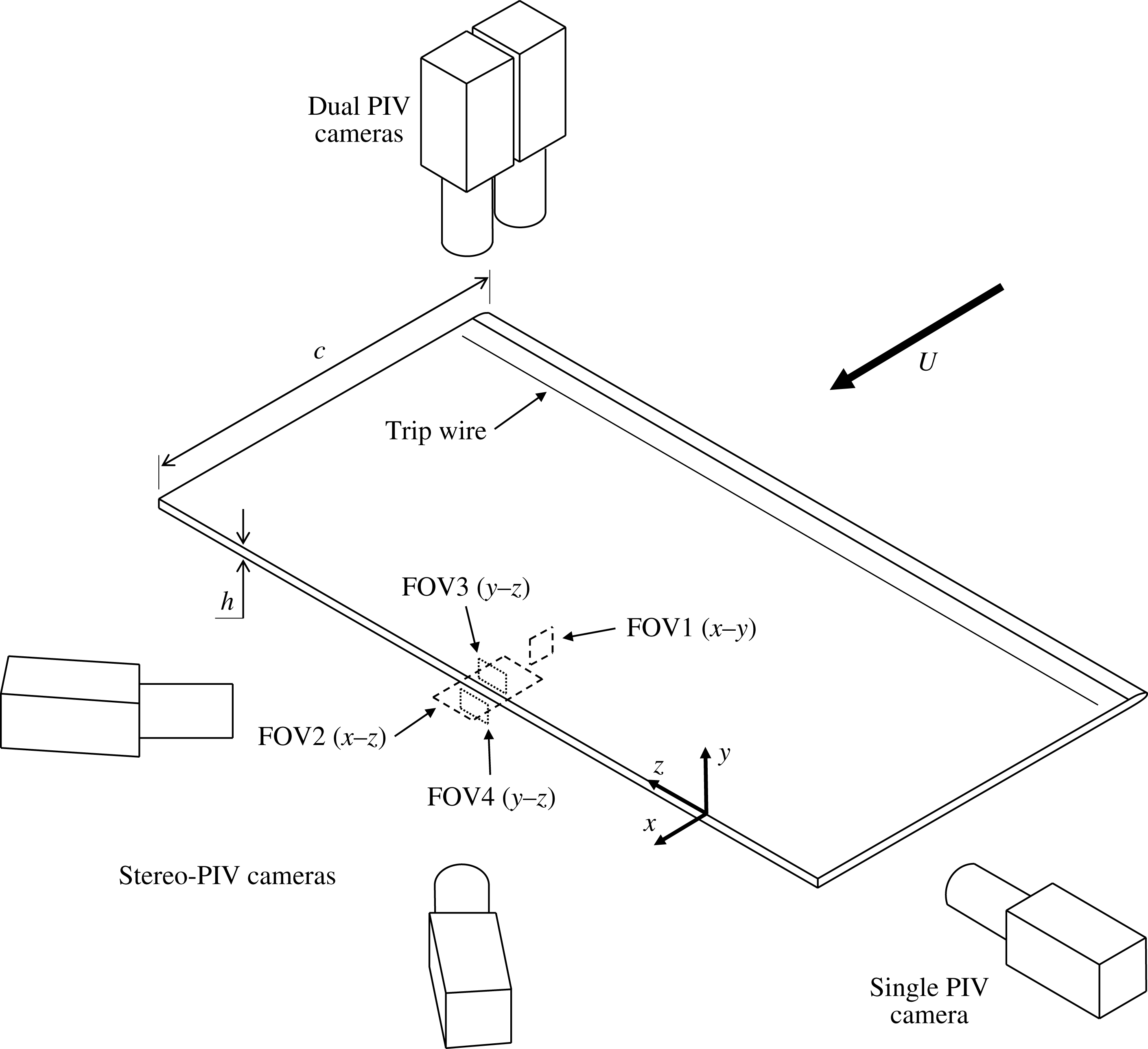
The elongated blunt body model was machined from an aluminium plate and sanded to a fine surface finish. It has a BTE height $h=12.9~\text{mm}$ and a chord length $c=600~\text{mm}$ , resulting in an aspect ratio of $AR=46.5$ . The leading edge was made semi-elliptical with a major to minor axis ratio of $5:1$ to prevent leading edge flow separation, and 1 mm tripping wires were attached to the surface 105 mm downstream from the leading edge on both sides of the model to uniformly trigger transition along the span. In the case of laminar flow, the perturbation caused by the wire was not amplified. The model was oriented at zero angle of attack, spanning the entire 1.2 m from floor to ceiling to produce a blockage ratio of 0.5 %. The elongated blunt body model can be viewed in figure 1.

Figure 1.

Schematic of the particle image velocimetry configurations and viewing regions. Note that $z=0$ is located at centre span. The axis is offset here for clear viewing of the imaging planes. The model has a BTE height $h=12.9~\text{mm}$ and a chord length $c=600~\text{mm}$ .

2.2 Two-component particle image velocimetry

A 2C-PIV system was utilised in two configurations to measure instantaneous velocity fields of the upstream boundary layer in the $x$ – $y$ plane (denoted as FOV1) and the low-speed zones near the BTE in the $x$ – $z$ plane (denoted as FOV2). The illumination was provided by an Nd:YAG laser (Spectra-Physics, PIV-400-10) that is capable of outputting 532 nm light at 400 mJ per pulse with a pulse width of 5–8 ns. The laser beam was shaped using one negative cylindrical and two spherical lenses to produce a laser sheet with a thickness of 1 mm. The resulting laser sheet was then directed as necessary using several adjustable mirrors. Imager ProX-4M cameras were used to collect images, each featuring a $2048\times 2048$ -pixel CCD sensor with a $7.4\times 7.4~\unicode[STIX]{x03BC}\text{m}^{2}$ pixel size and 14-bit resolution. A schematic representation of the 2C-PIV set-up is included in figure 1.

The boundary layer within FOV1 was imaged at a distance of 7 $h$ upstream from the BTE at centre span. A Nikon lens with a focal length of $f=200~\text{mm}$ and an aperture setting of $f/5.6$ was utilised with the camera which was set 0.7 m from the viewing plane, resulting in a digital resolution of $20.5~\unicode[STIX]{x03BC}\text{m}~\text{pix}^{-1}$ and a streamwise–wall-normal FOV of $(\unicode[STIX]{x0394}x,\unicode[STIX]{x0394}y)=42\times 42~\text{mm}^{2}$ ( $3.3h\times 3.3h$ ). The flow was seeded with ${\sim}1~\unicode[STIX]{x03BC}\text{m}$ particles using a fog generator, and then 500 double-frame images were collected at a frequency of 4 Hz for each flow speed considered.

The low-speed zones in the boundary layer and wake regions of the flow were measured using FOV2 in the $x$ – $z$ plane at $y=1.5~\text{mm}$ above the surface. Two cameras were fitted with identical Nikon lenses, each with $f=200~\text{mm}$ and aperture settings of $f/8.4$ . They were placed side by side at a distance of 1.3 m from the viewing plane. The digital resolutions of the upstream and downstream cameras were 34.4 and $34.2~\unicode[STIX]{x03BC}\text{m}~\text{pix}^{-1}$ , respectively, and the viewing regions overlapped by 5 mm so that the resulting vector fields could be stitched together. The combined streamwise–spanwise FOV had dimensions of $(\unicode[STIX]{x0394}x,\unicode[STIX]{x0394}z)=135\times 70~\text{mm}^{2}$ (10.5 $h$   $\times$  5.4 $h$ ) centred at $x=0$ and at centre span. After seeding with ${\sim}1~\unicode[STIX]{x03BC}\text{m}$ fog particles, sets of 5000 double-frame images were collected by both cameras simultaneously at a frequency of 4 Hz for each flow speed considered.

The images were processed using DaVis 8.2 software (LaVision GmbH). First, a preprocessing step was necessary to improve image quality. The minimum of each ensemble was subtracted to remove background noise, followed by normalisation using ensemble averages. FOV1 was imaged to obtain mean velocity profiles, and so an ensemble of correlation was applied to these sets (Meinhart, Wereley & Santiago Reference Meinhart, Wereley and Santiago2000). A multi-pass algorithm was used with $24\times 24$ -pixel ( $0.49\times 0.49$ -mm) interrogation windows with 75 % overlap for the final pass. A $4:1$ elliptical Gaussian distribution was applied to the window with the major axis of the ellipse in the streamwise direction to improve the correlation. FOV2 was processed using a standard multi-pass cross-correlation with the final passes utilising Gaussian $48\times 48$ -pixel ( $1.65\times 1.65$ -mm) interrogation windows with 75 % overlap. A postprocessing step was applied to the wake ensembles using universal outlier detection (Westerweel & Scarano Reference Westerweel and Scarano2005) and linear interpolation to account for incorrect and missing vectors, which made up less than 1 % of each vector field.

2.3 Stereoscopic particle image velocimetry

The wake and boundary layer regions were characterised using two different stereo-PIV systems. The first system utilises the same laser and cameras as the 2C-PIV experiments and the second is high-speed for collecting time-resolved images. The high-speed system makes use of a dual-cavity Nd:YLF laser (Photonics Industries, DM20-527-DH) at 527 nm with a maximum frequency of 10 kHz. The combined beam of the two laser cavities is capable of outputting a maximum of 40 mJ per pulse (at 1 kHz) with a pulse width of 170 ns. Two Phantom v611 high-speed cameras were utilised, each with a $1280\times 800$ -pixel CMOS sensor with a $20\times 20~\unicode[STIX]{x03BC}\text{m}^{2}$ pixel size and 12-bit resolution. The first stereoscopic $y$ – $z$ viewing plane (denoted as FOV3) was located 0.3 $h$ upstream from the BTE location at centre span and began at the surface of the model ( $y=0$ ). The second stereoscopic $y$ – $z$ viewing plane (denoted as FOV4) was centred at $y=-0.5h$ and located 2 $h$ downstream from the BTE location as shown in figure 1.

Snapshots of the flow in FOV3 and FOV4 were captured for statistical analysis with higher spatial resolution. The mean flow direction was perpendicular to these viewing planes and so the second laser sheet pulse was moved 0.5 mm downstream from the first in both FOV3 and FOV4 to improve the number of common particles captured between frames. Each laser sheet pulse had a thickness of 1.5 mm using the same combination of optics as used previously, resulting in a total laser sheet thickness of 2 mm centred at $x=-0.3h$ for FOV3 and at $x=2h$ for FOV4. The stereo-PIV cameras were each set approximately 1 m from the FOVs and were fit with Scheimpflug mounts and Nikon lenses with $f=200~\text{mm}$ . An aperture setting of $f/11$ was used on the forward scattering camera, while a setting of $f/8.4$ was used on the camera with a backward scattering orientation. A two-step stereoscopic calibration process was used for both FOVs which included a three-dimensional target calibration followed by self-calibration with a small set of particle images (Wieneke Reference Wieneke2005). The spanwise–wall-normal FOV was $(\unicode[STIX]{x0394}z,\unicode[STIX]{x0394}y)=76\times 61~\text{mm}^{2}$ (5.9 $h$   $\times$  4.7 $h$ ) with a digital resolution of $28.8~\unicode[STIX]{x03BC}\text{m}~\text{pix}^{-1}$ and a residual error of 0.06 pix for FOV3. A spanwise–wall-normal FOV of $(\unicode[STIX]{x0394}z,\unicode[STIX]{x0394}y)=75\times 59~\text{mm}^{2}$ (5.8 $h$   $\times$  4.6 $h$ ) with a digital resolution of $28.1~\unicode[STIX]{x03BC}\text{m}~\text{pix}^{-1}$ and a residual error of 0.06 pix was obtained for FOV4. The flow was seeded with ${\sim}1~\unicode[STIX]{x03BC}\text{m}$ particles using a fog generator and 5000 double-frame images were collected from each camera simultaneously at a frequency of 4 Hz for each flow speed considered and in both FOV3 and FOV4.

High-speed stereoscopic measurements were also conducted within FOV4 for the purpose of studying the temporal evolution of the vortices in the wake. The laser sheet was made to be 2 mm thick using the same combination of optics as before. The high-speed cameras were placed in the same location as the Imager ProX cameras in the previous stereoscopic experiment and with the same lenses and aperture settings. The previously mentioned stereoscopic calibration procedure was followed, resulting in a spanwise–wall-normal FOV of $(\unicode[STIX]{x0394}z,\unicode[STIX]{x0394}y)=115\times 58~\text{mm}^{2}$ (8.9 $h$   $\times$  4.5 $h$ ) with a digital resolution of $71.6~\unicode[STIX]{x03BC}\text{m}~\text{pix}^{-1}$ and a residual error of 0.02 pix. Ensembles of 5400 time-resolved images were collected at an acquisition frequency of 6.2 kHz for each flow speed considered.

All images were once again processed using DaVis 8.2. The double-frame stereo-PIV images were cross-correlated using multiple passes, the last of which utilised Gaussian $96\times 96$ -pixel ( $2.70\times 2.70$ -mm) interrogation windows with 75 % overlap. A postprocessing step was then applied which removed and replaced outliers and interpolated missing vectors. The incorrect and missing vectors accounted for less than 4 % of each vector field. The high-speed stereo-PIV images were processed using a sliding ensemble-of-correlation algorithm with a filter length of 5 images using 4 successive pairs each with a time separation of $\unicode[STIX]{x0394}t=161~\unicode[STIX]{x03BC}\text{s}$ to reduce random, high-frequency noise (Ghaemi, Ragni & Scarano Reference Ghaemi, Ragni and Scarano2012). The operation utilised a multi-pass cross-correlation with final Gaussian $48\times 48$ -pixel ( $3.44\times 3.44$ -mm) interrogation windows with 75 % overlap. No postprocessing was performed on the resulting time-resolved vector fields.

3.1 Upstream boundary layer development

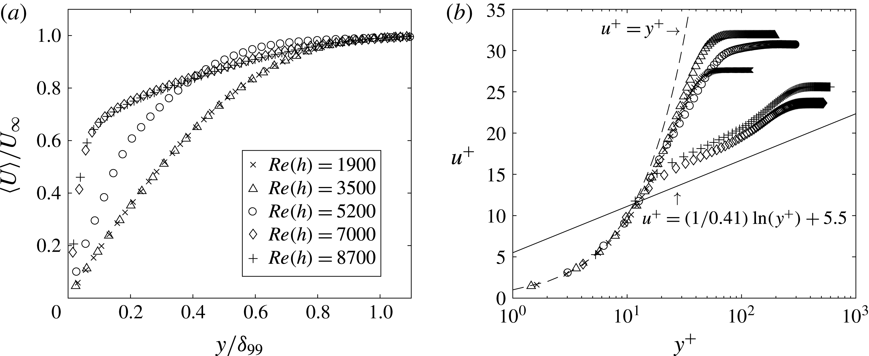
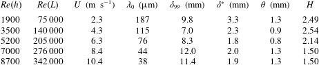
The mean boundary layer profiles 7 $h$ upstream from the BTE are presented on both linear and semi-logarithmic axes in figures 2(a) and 2(b), respectively. The high spatial resolution of the 2C-PIV measurements from the ensemble-of-correlation technique in FOV1 allowed for calculation of the inner layer scales, including the wall unit $\unicode[STIX]{x1D706}_{0}$ , by fitting a line to the linear viscous sublayer of the mean profiles. The state of the upstream boundary layer is summarised in table 1. By inspection of figure 2(a) and the calculated shape factors ( $H$ , the ratio of displacement thickness to momentum thickness) in table 1, it is evident that the upstream boundary layer is laminar for $Re(h)=1900$ and 3500, transitional for $Re(h)=5200$ and turbulent for $Re(h)=7000$ and 8700.

It can be seen in figure 2(b) that the turbulent boundary layer profiles at $Re(h)=7000$ and 8700 do not follow the standard logarithmic ‘law of the wall’ for a zero pressure gradient (ZPG) turbulent boundary layer. In fact, both turbulent profiles clearly exceed the logarithmic line. This deviation can be attributed to the favourable pressure gradient (FPG) caused by the low-pressure near-wake region of the body. This mean profile behaviour is typical of FPG turbulent boundary layers due to their tendency to accelerate and relaminarise, causing the semi-logarithmic profiles to shift towards the laminar curves (Patel & Head Reference Patel and Head1968; Badri Narayanan & Ramjee Reference Badri Narayanan and Ramjee1969; Blackwelder & Kovasznay Reference Blackwelder and Kovasznay1972). This flow acceleration has been confirmed near the BTE using PIV measurements; however, the results have been omitted for brevity. The remainder of this investigation will only consider $Re(h)=3500$ , 5200 and 7000 as the laminar, transitional and turbulent cases, respectively, to study the effect that a transitioning upstream boundary layer may have on the wake.

Figure 2.

Mean velocity profiles 7 $h$ upstream of the BTE (FOV1) plotted using (a) linear and (b) semi-logarithmic axes. Both sets of profiles have been decimated by a factor of 2 to improve visibility of the data points. The direct overlap between laminar and turbulent profiles in (a) reveals that the flow is fully laminar at $Re(h)=3500$ and fully turbulent at $Re(h)=7000$ . This is also concluded from the shape factors ( $H$ ) provided in table 1.

Table 1.

Parameters relating to the mean velocity profiles located 7 $h$ upstream from the BTE (from FOV1 in figure 1). Note that $L$ is the length of the model up to where these parameters were evaluated.

3.2 Secondary instability wavelength

The spanwise distance between adjacent counter-rotating streamwise vortex pairs within the wake region must be determined to characterise the secondary instability modes. This distance is also known as the secondary instability wavelength, as described previously, and will be denoted as $\unicode[STIX]{x1D706}_{z}$ . The streamwise wake vortices have been identified from the stereoscopic snapshots of FOV4 using the two-dimensional $Q$ -criterion (Jeong & Hussain Reference Jeong and Hussain1995), where the partial derivative terms have been evaluated using a second-order central differencing scheme. 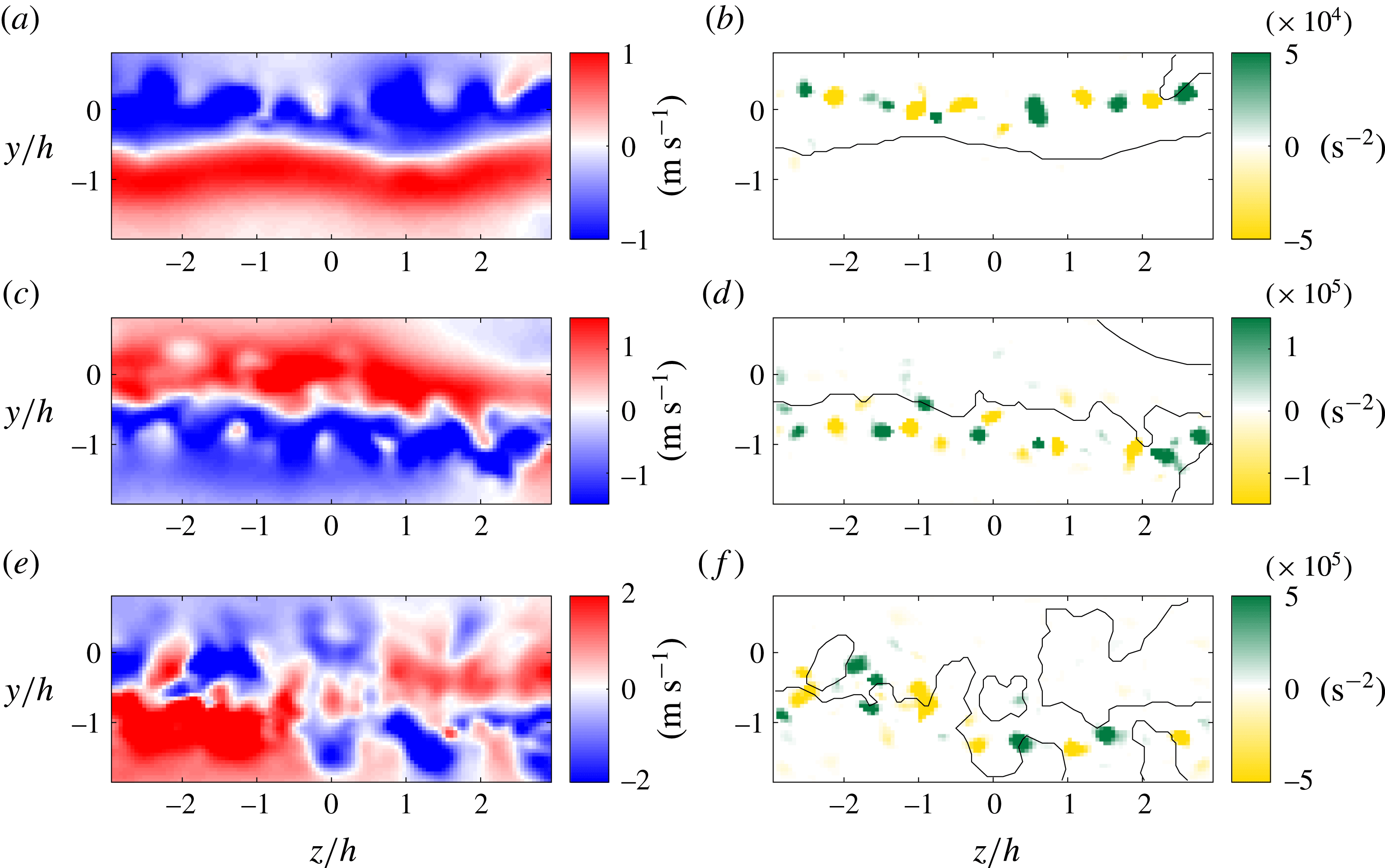All vortices, which are specified as regions of flow with $Q>0$ , were assigned a direction of rotation using the sign of streamwise vorticity ( $\unicode[STIX]{x1D714}_{x}$ ), and all $Q<0$ were discarded. This was done to facilitate identification of the counter-rotating vortex pairs from within the stereoscopic snapshots. Sample snapshots of the fluctuating component of streamwise velocity ( $u^{\prime }$ ) and the corresponding modified $Q$ -criterion ( $Q^{\prime }=\unicode[STIX]{x1D714}_{x}Q/|\unicode[STIX]{x1D714}_{x}|$ ) are provided in figure 3 for $Re(h)=3500$ , 5200 and 7000. These samples have been selected at instances when the stereo-PIV plane was cutting through one of the primary spanwise vortices to emphasise the location of the streamwise vortex pairs with respect to the primary vortex cores.

Figure 3.

Instantaneous snapshots of the fluctuating component of streamwise velocity ( $u^{\prime }$ ) and the corresponding modified $Q$ -criterion ( $Q^{\prime }=\unicode[STIX]{x1D714}_{x}Q/|\unicode[STIX]{x1D714}_{x}|$ ) in the wake at $x=2h$ for (a,b) $Re(h)=3500$ , (c,d) $Re(h)=5200$ and (e,f) $Re(h)=7000$ . The $u^{\prime }=0$ lines have been added to the contour plots of $Q^{\prime }$ to facilitate comparison between plots. The streamwise vortex pairs tend to exist either on the $u^{\prime }=0$ line or in the region of the flow with $u^{\prime }<0$ . The high-speed data within FOV4 have been used to create animations of the streamwise vortices visible in (b), (d) and (f). These videos can be found in the supplementary material as movies 1, 2 and 3, respectively available at https://doi.org/10.1017/jfm.2018.285.

Figure 3(a,c) reveals a clear divide between positive and negative $u^{\prime }$ at $Re(h)=3500$ and 5200. This divide occurs where the fluid has no out-of-plane motion with respect to the advecting frame of reference and is represented as a white line separating the red and blue regions of flow corresponding to positive and negative regions of $u^{\prime }$ , respectively. The divide exists due to the rotation of the primary spanwise vortices, as they contain fluid moving both with ( $u^{\prime }>0$ ) and against ( $u^{\prime }<0$ ) the advecting frame of reference as the vortex moves downstream. In contrast, the isocontour of $u^{\prime }=0$ for $Re(h)=7000$ in figure 3(e) is highly jagged with engulfed regions of opposite velocity fluctuation on either side of the wake centre line ( $y=-0.5h$ ). This is caused by intense distortion of the primary spanwise vortices as $Re$ increases. Distortion of the primary vortices can be found throughout the collected data and becomes more prevalent as $Re$ is increased.

The counter-rotating streamwise vorticity pattern of the secondary instability is easily identified in the stereoscopic snapshots of $Q^{\prime }$ presented in figure 3(b,d,f). By comparison between the snapshots of $u^{\prime }$ and $Q^{\prime }$ , it is evident that the streamwise vortices of the secondary instability tend to exist either on the $u^{\prime }=0$ line or in the region of the wake with $u^{\prime }<0$ . As previously mentioned, the latter corresponds to the portion of the primary spanwise vortex that is rotating upstream with respect to the advecting frame of reference. This streamwise vortex placement persists when the wake is distorted as can be seen in figure 3(f). The jagged interface between positive and negative $u^{\prime }$ brings a similar jaggedness to the spanwise sequence of secondary vortices, with the streamwise vortices continuing to exist either on the $u^{\prime }=0$ line or in the region with $u^{\prime }<0$ . This behaviour of secondary vortex pairs is consistent with the simplified mode B model that has been proposed by Brede et al. (Reference Brede, Eckelmann and Rockwell1996) for the cylinder wake. Their model features simply connected streamwise vortex tubes which weave between primary spanwise vortices, always passing around the side of the primary vortex that is rotating towards the upstream direction. The streamwise vortices alternate sign in the spanwise direction, therefore existing in counter-rotating pairs, and have a secondary instability wavelength of approximately 1 $d$ as determined by their experiments. A similar model has been given by Williamson (Reference Williamson1996a ); however, the author stated that it was not obvious that the streamwise vortices were simply connected.

The spanwise distance between adjacent streamwise vortex pairs in the present stereoscopic snapshots has been calculated using a spatial autocorrelation in the spanwise direction. The operation has been applied to the snapshots of $Q^{\prime }$ . The autocorrelation coefficient of the $i$ th snapshot shifted in the spanwise direction by $\unicode[STIX]{x0394}z$ is given by

(3.1) $$\begin{eqnarray}C(\unicode[STIX]{x0394}z)=\frac{\langle Q^{\prime }(y_{0},z_{0},t_{i})\cdot Q^{\prime }(y_{0},z_{0}+\unicode[STIX]{x0394}z,t_{i})\rangle }{Q_{rms}^{\prime }(y_{0},z_{0},t_{i})Q_{rms}^{\prime }(y_{0},z_{0}+\unicode[STIX]{x0394}z,t_{i})},\end{eqnarray}$$

where the subscript rms denotes the root-mean-square operation. The distance between adjacent vortex pairs within each snapshot was then taken to be twice the distance between the initial maximum value ( $C(0)=1$ ) and the first minimum of the respective autocorrelation. This minimum occurs when the snapshot has been shifted such that vortices with opposite signs align, and therefore it represents a distance that is half that of the secondary instability wavelength.

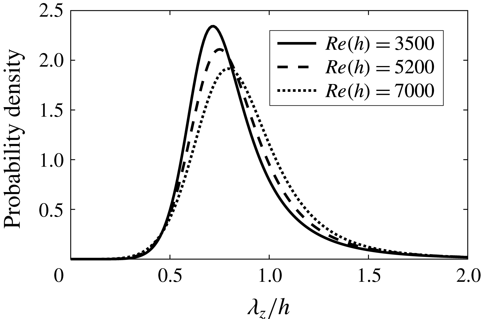
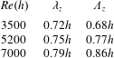
The process described above has been applied to all stereo-PIV ensembles. Probability density functions (PDFs) that have been fit to the resulting values of $\unicode[STIX]{x1D706}_{z}$ using a Burr type XII distribution (Tadikamalla Reference Tadikamalla1980) are shown in figure 4. By inspection, each PDF of $\unicode[STIX]{x1D706}_{z}$ is unimodal and slightly right-skewed. 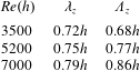The peaks represent estimates for the most probable values of $\unicode[STIX]{x1D706}_{z}$ and correspond to 0.72 $h$ , 0.75 $h$ and 0.79 $h$ for $Re(h)=3500$ , 5200 and 7000, respectively. These values for $\unicode[STIX]{x1D706}_{z}$ closely match the secondary instability wavelength of mode B found in the wakes of cylinders (Williamson Reference Williamson1996b ) and the predicted wavelength of mode S $^{\prime }$ for the wake of an elongated blunt body (Ryan et al. Reference Ryan, Thompson and Hourigan2005). The distributions do not change significantly as the flow upstream from the BTE transitions from laminar to turbulent; however, a reduction in magnitude and shift of the peak to the right is visible. Each distribution being unimodal suggests that there is only one dominant mode in the wake for the investigated $Re$ . Additionally, any dominant presence of the BTE mode B $^{\prime }$ in the wake can be ruled out, as it has a secondary instability wavelength closer to 2.2 $h$ .

Figure 4.

Probability density functions of secondary instability wavelength ( $\unicode[STIX]{x1D706}_{z}$ ) in the wake at $x=2h$ for $Re(h)=3500$ , 5200 and 7000. The wavelengths were obtained by spatial correlation of vortex cores identified using a modified $Q$ -criterion ( $Q^{\prime }=\unicode[STIX]{x1D714}_{x}Q/|\unicode[STIX]{x1D714}_{x}|$ ) as described by (3.1).

3.3 Temporal behaviour of the streamwise wake vortices

The organisation of the streamwise vortices in the wake must be determined to further characterise the secondary instability. In particular, knowledge of how the vortices relate from one primary shedding cycle to the next is required to distinguish between the cylinder mode B and the BTE mode S $^{\prime }$ . The two modes have similar fine-scale spanwise wavelengths; however, the mode B secondary vortices maintain their direction of rotation over many shedding cycles while the mode S $^{\prime }$ secondary vortices change their direction of rotation between each cycle of the primary instability (Ryan et al. Reference Ryan, Thompson and Hourigan2005). In the previous subsection, it was determined that the most probable secondary instability wavelength for the $Re$ considered here is approximately $\unicode[STIX]{x1D706}_{z}=0.7h{-}0.8h$ . How the secondary vortices behave between primary shedding cycles is the last piece of information required to determine which mode is present in the wake.

High-speed stereo-PIV measurements have been performed within FOV4 at $x=2h$ and the resulting time-resolved sequences of vector fields have been used to investigate the temporal characteristics of the streamwise wake vortices. The modified $Q$ -criterion ( $Q^{\prime }=\unicode[STIX]{x1D714}_{x}Q/|\unicode[STIX]{x1D714}_{x}|$ ) has been determined as described in § 3.2 to identify the streamwise vortex pairs within each stereoscopic velocity field. 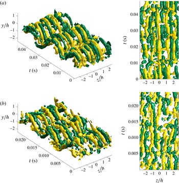The resulting time-resolved evolution of $Q^{\prime }$ has been obtained by stacking the two-dimensional plots along the third dimension (i.e. time) to facilitate visualisation of the vortical structures as they evolve temporally. Isosurface constructions of the vortical structures within the wake at $x=2h$ are given in figure 5 for $Re(h)=3500$ and 7000. These plots are representative of the wake behaviour contained in all high-speed data collected in this study.

Figure 5.

Isosurface constructions of modified $Q$ -criterion ( $Q^{\prime }=\unicode[STIX]{x1D714}_{x}Q/|\unicode[STIX]{x1D714}_{x}|$ ) in the wake at $x=2h$ for (a) $Re(h)=3500$ (isosurface at $Q^{\prime }=\pm 2000~\text{s}^{-2}$ ) and (b) $Re(h)=7000$ (isosurface at $Q^{\prime }=\pm 18\,000~\text{s}^{-2}$ ). Green and gold represent positive and negative rotational directions, respectively. Isosurface values have been chosen to obtain clear visualisations. Lowering the value makes the plots denser but does not alter the patterns displayed. Note that a second-order regression filter with a kernel size of 5 has been applied to the data to reduce noise and facilitate visualisation.

The alternating sign of vorticity in the spanwise direction is highly visible in the isosurface constructions in figure 5. Additionally, it is straightforward to see by visual inspection that many of the streamwise vortices in figure 5(a) maintain their direction of rotation over the primary shedding cycles presented in the figure. This is not as easily visualised at higher $Re$ when the wake region becomes more turbulent and three-dimensional. Thus, visual inspection of the vortex samples needs to be verified by statistical analysis. This has been done using a spatial cross-correlation in the spanwise direction, applied to the reconstructed temporal evolution of $Q^{\prime }$ . Subsequent vortex shedding cycles have been isolated as three-dimensional matrices and cross-correlated to determine whether the vortices change their direction of rotation between primary cycles. If the vortices maintain their rotational directions, the cross-correlation coefficient will begin at a positive value at $\unicode[STIX]{x0394}z=0$ and trend towards a minimum with increasing $\unicode[STIX]{x0394}z$ . This minimum will occur at a value of approximately $\unicode[STIX]{x0394}z=\unicode[STIX]{x1D706}_{z}/2$ due to the alignment of vortices with opposite directions of rotation after the shift. However, the opposite will be true if the vortices are to change rotational direction between primary shedding cycles, i.e. the cross-correlation coefficient will begin at a minimum due to the alignment of vortices with opposite rotation and trend towards a maximum value at the location $\unicode[STIX]{x0394}z=\unicode[STIX]{x1D706}_{z}/2$ where the vortices with the same rotational direction now align. This process has been applied to all $N$ vortex shedding cycles for each $Re$ considered and the resulting cross-correlation curves have been averaged. The mathematical description of the operation is given by

(3.2) $$\begin{eqnarray}\unicode[STIX]{x1D70C}(\unicode[STIX]{x0394}z)=\frac{1}{N-1}\mathop{\sum }_{i=1}^{N-1}\frac{\langle Q^{\prime }(y_{0},z_{0},t_{i})\cdot Q^{\prime }(y_{0},z_{0}+\unicode[STIX]{x0394}z,t_{i}+T_{shed})\rangle }{Q_{rms}^{\prime }(y_{0},z_{0},t_{i})Q_{rms}^{\prime }(y_{0},z_{0}+\unicode[STIX]{x0394}z,t_{i}+T_{shed})},\end{eqnarray}$$

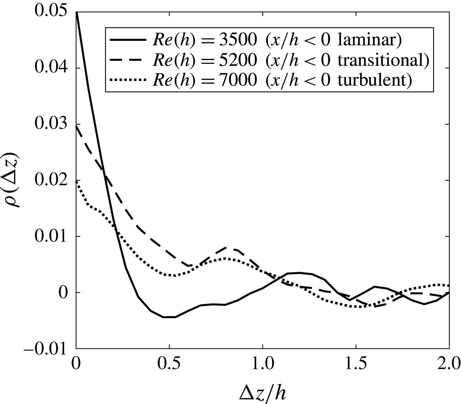
where $T_{shed}$ is the period of the primary vortex shedding cycle and $Q^{\prime }$ is a three-dimensional matrix containing a complete shedding cycle. The results for $Re(h)=3500$ , 5200 and 7000 are given in figure 6. In agreement with the instantaneous visualisations in figure 5, the averaged cross-correlation curves reveal that the streamwise vortices maintain their direction of rotation during primary shedding cycles since a maximum peak is observed at $\unicode[STIX]{x0394}z=0$ . Moreover, the first minimum in each plot occurs at approximately $\unicode[STIX]{x0394}z/h=0.5$ , confirming that the mean secondary instability wavelength is near $\unicode[STIX]{x1D706}_{z}=1h$ for the considered $Re$ and therefore matches that of the cylinder mode B.

Figure 6.

Average of spanwise cross-correlations applied to three-dimensional modified $Q$ -criterion ( $Q^{\prime }=\unicode[STIX]{x1D714}_{x}Q/|\unicode[STIX]{x1D714}_{x}|$ ) between all subsequent primary vortex shedding cycles following equation (3.2). All cross-correlation curves begin at a maximum positive value, indicating that the vortex pairs maintain their directions of rotation during primary shedding cycles. The first minimum of each curve is near $\unicode[STIX]{x0394}z/h=0.5$ , providing further evidence that the secondary instability wavelength is close to $\unicode[STIX]{x1D706}_{z}=1h$ .

Upon further inspection of the isosurface constructions in figure 5, it is evident that the streamwise vortices maintain their spanwise positions over time. This behaviour agrees with the models proposed by Brede et al. (Reference Brede, Eckelmann and Rockwell1996) and Williamson (Reference Williamson1996a ) for the circular cylinder mode B; however, the behaviour contradicts the model proposed by Naghib-Lahouti et al. (Reference Naghib-Lahouti, Doddipatla and Hangan2012) for the secondary instability in the wake of an elongated blunt body at a smaller $AR$ of 12.5 based on LIF visualisations and reconstructed velocity fields. Their blunt body model contains streamwise vortices which stagger their spanwise positions every half-shedding cycle, which is not observed here. Moreover, the streamwise vortices in figure 5(a) appear to be simply connected as modelled by Brede et al. (Reference Brede, Eckelmann and Rockwell1996), although it is difficult to confirm whether this behaviour is persistent in the wake.

Thus far, all results presented regarding the secondary wake vortices suggest that the cylinder mode B is the dominant secondary instability within the wake of the elongated blunt body studied here with $AR=46.5$ for $Re(h)=3500$ , 5200 and 7000. No evidence of the BTE mode B $^{\prime }$ nor S $^{\prime }$ has been found within the collected data, as was anticipated from the stability analysis of Ryan et al. (Reference Ryan, Thompson and Hourigan2005) for $2.5\leqslant AR\leqslant 17.5$ and a maximum $Re(h)$ of 700 and the experimental work of Naghib-Lahouti et al. (Reference Naghib-Lahouti, Doddipatla and Hangan2012, Reference Naghib-Lahouti, Lavoie and Hangan2014) for $AR=12.5$ and $250\leqslant Re(h)\leqslant 5\times 10^{4}$ , although we would like to emphasise the large differences in $AR$ between these studies and the present investigation. The visual inspection and spatial-correlation analysis of both the time-resolved and statistical stereo-PIV data have been used to reach this conclusion.

3.4 Low-speed zones of streamwise velocity

Both the upstream boundary layer and the wake region feature low-speed zones of streamwise velocity fluctuation. In the boundary layer they are often referred to as streaks due to their streamwise elongation, and they exist when the flow is turbulent or transitioning to turbulence. The boundary layer streaks are directly related to streamwise vortices near the wall (Blackwelder & Eckelmann Reference Blackwelder and Eckelmann1979; Schoppa & Hussain Reference Schoppa and Hussain2002; Tomkins & Adrian Reference Tomkins and Adrian2003), and the spanwise distance between adjacent low-speed streaks in a ZPG turbulent boundary layer ranges from 90 to 140 wall units depending on the distance from the wall (Smith & Metzler Reference Smith and Metzler1983; Lin et al. Reference Lin, Laval, Foucaut and Stanislas2008). As previously mentioned, low-speed zones of streamwise velocity also exist in the wake when secondary instabilities are present and the spanwise distance between adjacent low-speed zones matches the secondary instability wavelength ( $\unicode[STIX]{x1D706}_{z}$ ) in the wake (Mansy et al. Reference Mansy, Yang and Williams1994; Wu et al. Reference Wu, Sheridan, Welsh and Hourigan1996). The low-speed zones in the boundary layer and wake regions and their respective vorticity content will be investigated in this section. The spanwise distance between adjacent low-speed zones will be denoted as $\unicode[STIX]{x1D6EC}_{z}$ .

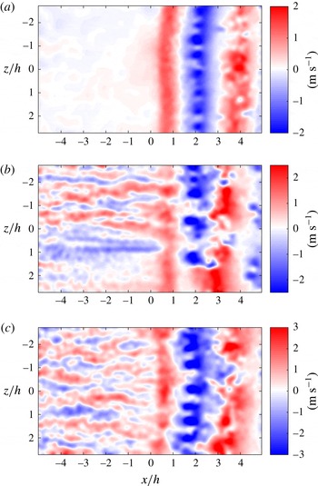
Sample snapshots of the fluctuating component of streamwise velocity ( $u^{\prime }$ ) are given in figure 7 for $Re(h)=3500$ , 5200, and 7000 from the stitched 2C-PIV measurements within FOV2. The respective laminar, transitional and turbulent nature of the upstream flow ( $x<0$ ) is evident within these snapshots. The fluctuation in streamwise velocity is almost non-existent in the upstream boundary layer in figure 7(a), as is expected for laminar flow. Conversely, the well-known turbulent boundary layer streaks are highly visible in figure 7(c), where both low- and high-speed streaks can be seen to have a continuous presence. The transitional nature of the flow in figure 7(b) is also evident, as boundary layer streaks are visible but do not populate the entire snapshot. Additionally, spanwise bands of low- and high-speed fluid are visible in the wake region ( $x>0$ ) of all snapshots. These bands represent slices through the primary spanwise vortices, resulting in low- and high-speed components which stem from the primary vortices that are rotating against and with the advecting frame of reference. The high-speed spanwise bands therefore represent primary vortices that have rolled off the near side of the BTE ( $y=0$ ) and the low-speed spanwise bands represent primary vortices that have rolled off the far side ( $y=-h$ ). The undulation of streamwise velocity in the spanwise direction (within the bands) is visible in all three snapshots, although it is more pronounced in the spanwise bands that have $u^{\prime }<0$ . This is consistent with the snapshots presented in figure 3, which revealed that the streamwise vortex pairs exist within the portion of each spanwise vortex that is rotating against advecting frame of reference (i.e. $u^{\prime }<0$ ). This once again agrees with the cylinder mode B models that have been presented by Brede et al. (Reference Brede, Eckelmann and Rockwell1996) and Williamson (Reference Williamson1996a ) and explains why the same undulating patterns are not visible in the spanwise bands with $u^{\prime }>0$ .

Figure 7.

Instantaneous fluctuating component of streamwise velocity ( $u^{\prime }$ ) in the $x$ – $z$ plane ( $y=1.5~\text{mm}$ ) for (a) $Re(h)=3500$ , (b) $Re(h)=5200$ and (c) $Re(h)=7000$ . The BTE is located at $x=0$ , and $x<0$ represents the upstream boundary layer while $x>0$ represents the wake. The respective laminar, transitional and turbulent states of the upstream boundary layers are evident in the snapshots. The spanwise bands of positive and negative $u^{\prime }$ in the wake represent the primary von Kármán vortices.

The spanwise distance between adjacent low-speed streaks in the upstream boundary layer was calculated using a spatial autocorrelation similar to the one described in § 3.2 and presented in (3.1). However, in the wake, the autocorrelation was only applied to the spanwise bands with $u^{\prime }<0$ that hold the undulating patterns. These bands do not have a continuous presence in a single streamwise location, and so a window of streamwise width $h$ (the height of the BTE) was used to search for the low-speed bands within each snapshot. The window was moved in the streamwise direction along the snapshots and the window with a minimum average velocity with respect to the rest of the snapshot was selected. The spanwise autocorrelation operation was applied to each window that was selected. The distance between adjacent low-speed zones was taken to be twice the distance between the initial maximum of the autocorrelation and the first minimum, and the centre of the window was considered the streamwise location of each corresponding autocorrelation result. The results were then binned at varying streamwise locations. The estimated $\unicode[STIX]{x1D6EC}_{z}$ in both the upstream boundary layer and wake have been fit with PDFs which are given in figure 8 for $Re(h)=3500$ , 5200 and 7000 and at various streamwise locations before and after the BTE. The PDFs were estimated using a Burr type XII distribution (Tadikamalla Reference Tadikamalla1980).

Figure 8.

Probability density functions of the distance between adjacent low-speed zones ( $\unicode[STIX]{x1D6EC}_{z}$ ) at $Re(h)=3500$ , 5200 and 7000 at streamwise locations (a) $x=-2h$ , (b) $x=-h$ , (c)  $x=0$ , (d) $x=h$ , (e) $x=2h$ and (f) $x=3h$ . The peak of each distribution represents the most probable value for $\unicode[STIX]{x1D6EC}_{z}$ at the corresponding streamwise location and $Re$ .

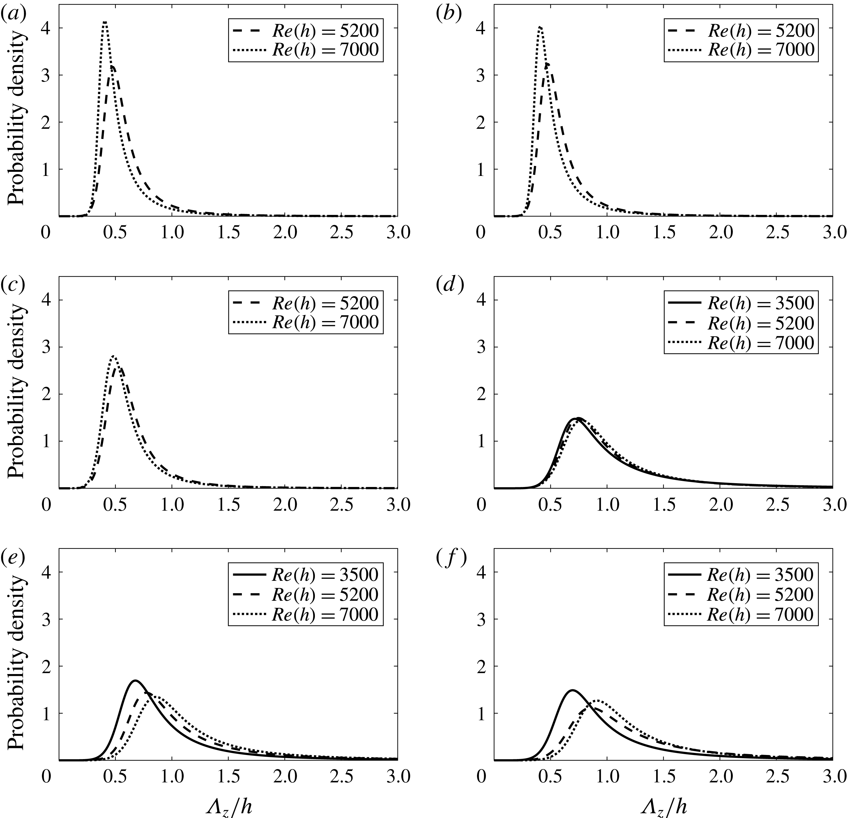
Similarly to the PDFs of $\unicode[STIX]{x1D706}_{z}$ in figure 4, all distributions of $\unicode[STIX]{x1D6EC}_{z}$ in figure 8 are unimodal and right-skewed. The peaks of the upstream boundary layer distributions (figure 8 a–c) are more distinct than those of the wake (figure 8 d–f), and it is generally observed that an increase in streamwise location brings a reduction in magnitude and shift of the peaks to the right. The most probable value for $\unicode[STIX]{x1D6EC}_{z}$ in the upstream turbulent boundary layer at $Re(h)=7000$ is approximately 0.41 $h$ based on the peaks of the PDFs at $x=-2h$ and $-h$ given in figures 8(a) and 8(b), respectively. Using the wall unit at $x=-7h$ presented in table 1 for $Re(h)=7000$ ( $\unicode[STIX]{x1D706}_{0}=44~\unicode[STIX]{x03BC}\text{m}$ ), this distance corresponds to $120\unicode[STIX]{x1D706}_{0}$ . This approximation falls within the expected range of 90 $\unicode[STIX]{x1D706}_{0}$ –140 $\unicode[STIX]{x1D706}_{0}$ for a ZPG turbulent boundary layer (Smith & Metzler Reference Smith and Metzler1983; Lin et al. Reference Lin, Laval, Foucaut and Stanislas2008), despite the FPG in this boundary layer. Using table 1 and the peaks in figure 8(a,b), the most probable value for $\unicode[STIX]{x1D6EC}_{z}$ in the transitional boundary layer at $Re(h)=5200$ is 81 $\unicode[STIX]{x1D706}_{0}$ .

The PDFs for $\unicode[STIX]{x1D6EC}_{z}$ in the wake at $x=2h$ (figure 8 $e$ ) are similar to the distributions for $\unicode[STIX]{x1D706}_{z}$ at the same location (figure 4). The most probable values for these distributions are compared in table 2, where it can be seen that the differences between $\unicode[STIX]{x1D706}_{z}$ and $\unicode[STIX]{x1D6EC}_{z}$ at $Re(h)=3500$ , 5200 and 7000 are relatively small and correspond to $-5.6\,\%$ , 3.1 % and 8.0 %, respectively, indicating that there is in fact a relationship between $\unicode[STIX]{x1D706}_{z}$ and $\unicode[STIX]{x1D6EC}_{z}$ . 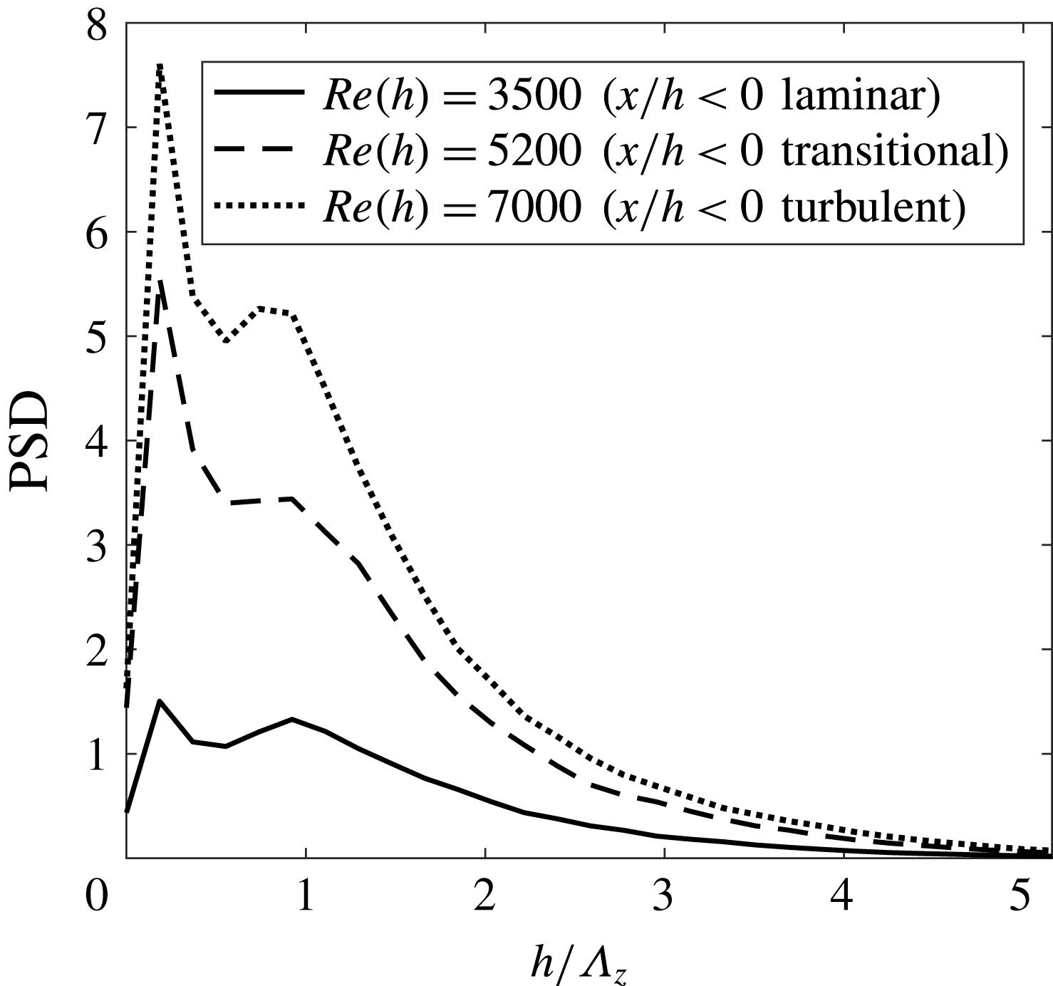The power spectral density (PSD) of $u^{\prime }$ at $x=2h$ has also been determined to further investigate $\unicode[STIX]{x1D6EC}_{z}$ in the wake and to validate the results of the autocorrelations, as the latter may have filtered out wavelengths with lower energy content. The central spanwise rows of $u^{\prime }$ have been extracted from the conditionally sampled spanwise bands of negative $u^{\prime }$ (the same windows that were autocorrelated to create the PDFs in figure 8 e). The data were multiplied with a Hanning window before PSD was calculated using a fast Fourier transform. The resulting spectra have been averaged and presented in figure 9 as PSD versus normalised wavenumber ( $h/\unicode[STIX]{x1D6EC}_{z}$ ). Each of the three spectra features two peaks at the same locations for each $Re$ . The first and second peaks correspond to $\unicode[STIX]{x1D6EC}_{z}=5.4h$ and 1.1 $h$ , respectively. The first value for $\unicode[STIX]{x1D6EC}_{z}$ matches the total spanwise length of FOV2 and is therefore not physical. The second value of $\unicode[STIX]{x1D6EC}_{z}=1.1h$ is close to the spanwise distances reported by the autocorrelations, thus validating the previous results. The absence of any other physical peak in the spectra strengthens the observation that the cylinder mode B is the only secondary instability present in the wake of the elongated blunt body studied here.

Table 2.

Most probable values for secondary instability wavelength ( $\unicode[STIX]{x1D706}_{z}$ ) and the spanwise distance between low-speed zones ( $\unicode[STIX]{x1D6EC}_{z}$ ) in the wake at $x=2h$ from the distributions given in figures 4 and 8(e), respectively.

Figure 9.

Power spectral densities of the spanwise signals of streamwise velocity fluctuation ( $u^{\prime }$ ) in the wake at $x=2h$ for $Re(h)=3500$ , 5200 and 7000. The first peak corresponds to the spanwise size of FOV2 and is therefore not physical. The second peak represents the secondary instability wavelength.

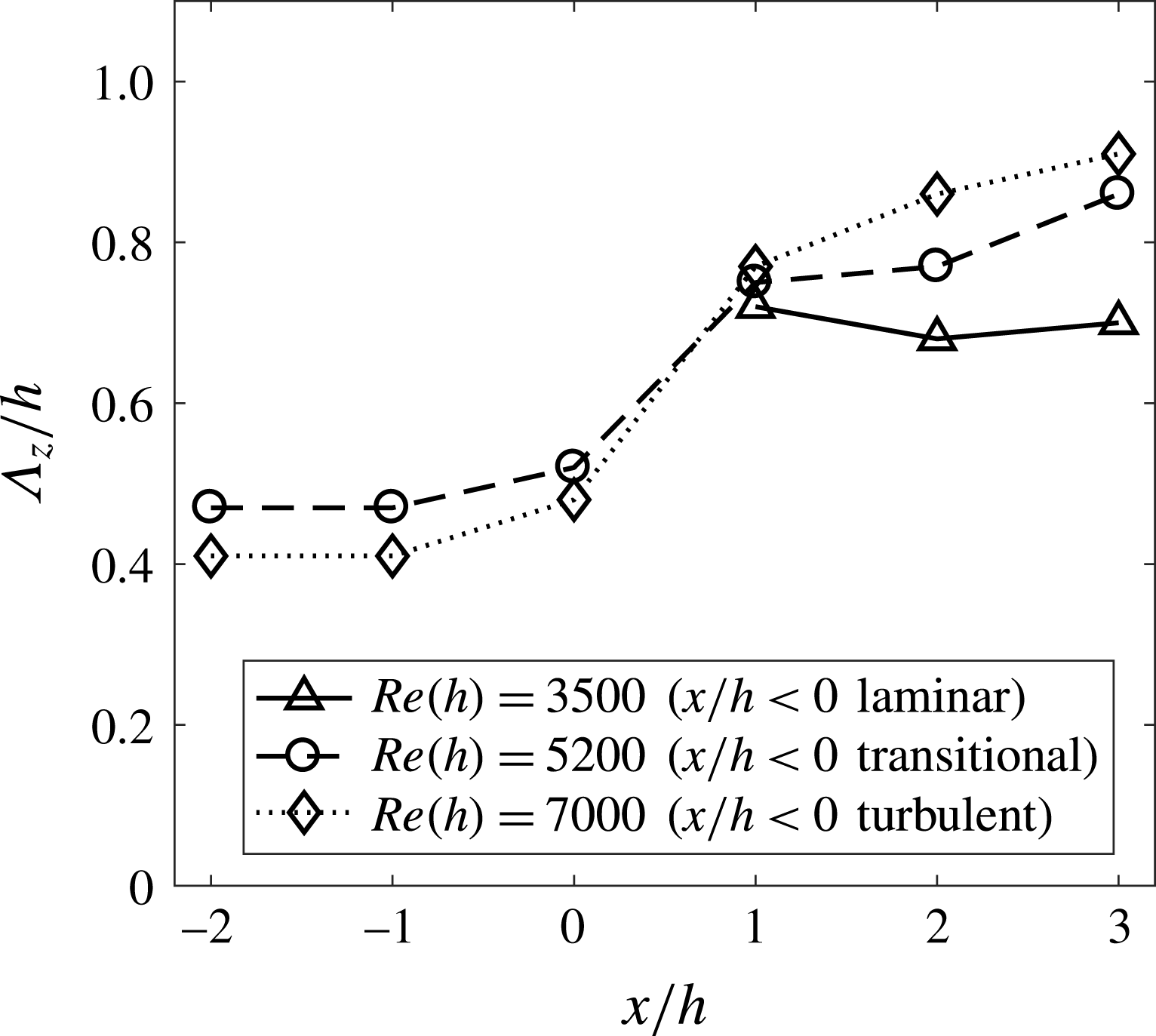
The most probable values from all PDFs in figure 8 are plotted as a function of distance from the BTE ( $x=0$ ) in figure 10. This has been done to facilitate characterisation of the evolution of the low-speed structures as they move from the upstream boundary layer and into the wake. Figure 10 reveals that the boundary layer streak spacing remains relatively constant before a rapid increase in $\unicode[STIX]{x1D6EC}_{z}$ over the range $0<x<h$ as the low-speed structures of the boundary layer are replaced by those of the unsteady wake. Beyond $x=h$ , $\unicode[STIX]{x1D6EC}_{z}$ stays relatively constant for $Re(h)=3500$ and continues to gradually increase for $Re(h)=5200$ and 7000.

Figure 10.

Most probable distance between adjacent low-speed zones ( $\unicode[STIX]{x1D6EC}_{z}$ ) as a function of distance from the BTE ( $x=0$ ) for $Re(h)=3500$ , 5200 and 7000. Each point represents the peak of the corresponding probability density functions given in figure 8. The rapid change in $\unicode[STIX]{x1D6EC}_{z}$ over the region $0<x/h<1$ is due to the boundary layer structures being replaced by the secondary instability.

As mentioned previously, the low-speed zones of streamwise velocity in both the upstream boundary layer and wake are related to the streamwise vorticity field. Whether the streamwise vortices present in the upstream boundary layer re-organise into the secondary wake vortices or are replaced altogether has been investigated using the stereo-PIV snapshots in the boundary layer at $x=-0.3h$ (FOV3) and the wake at $x=2h$ (FOV4). Two-dimensional $Q$ -criterion (Jeong & Hussain Reference Jeong and Hussain1995) has been used to identify vortices in the snapshots using a threshold to discard noise in the free stream ( $Q=3000~\text{s}^{-2}$ was chosen by inspection of numerous snapshots of $Q$ ). 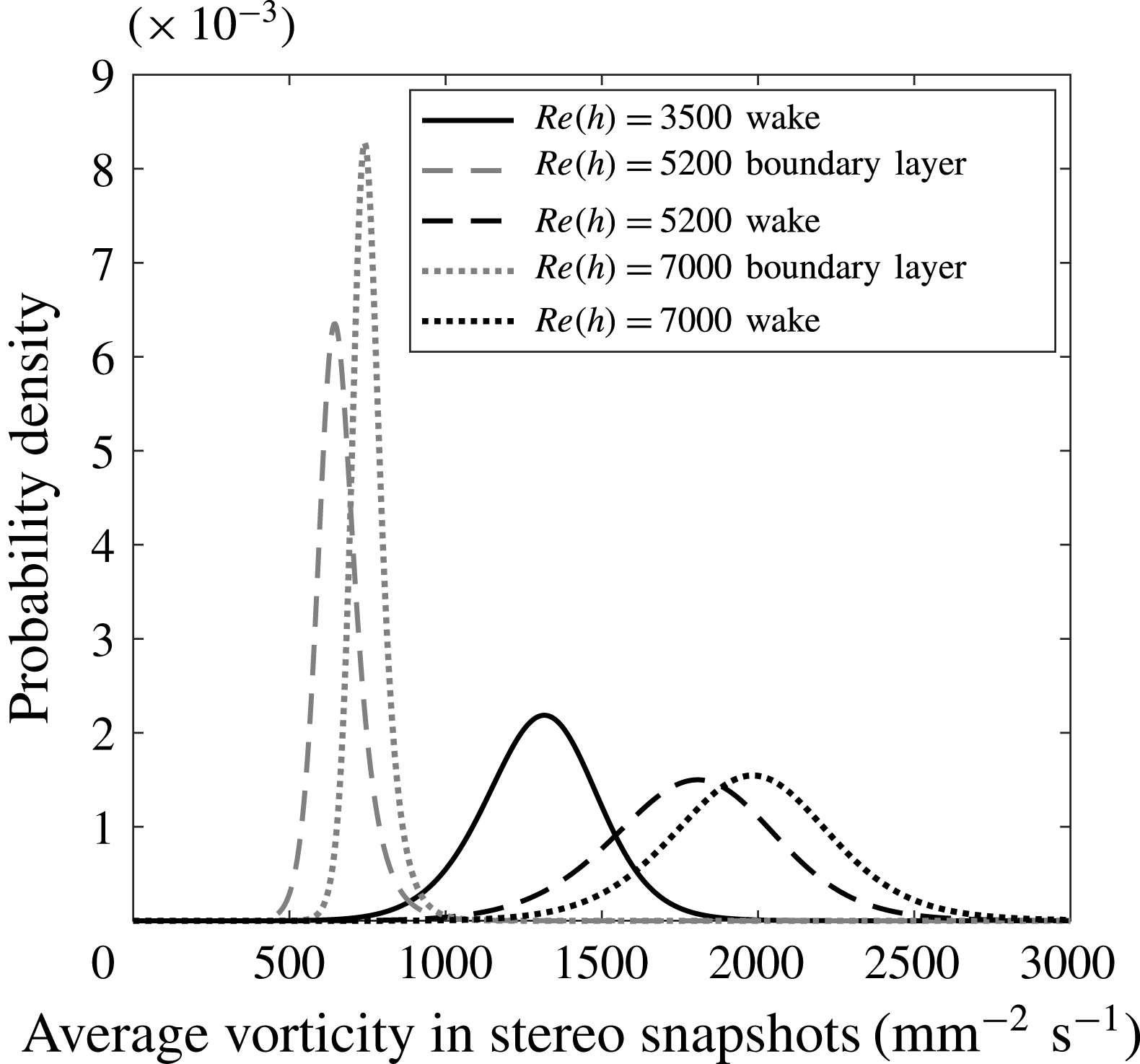The absolute values of streamwise vorticity ( $|\unicode[STIX]{x1D714}_{x}|$ ) in the conditionally selected vortex cores with $Q>3000~\text{s}^{-2}$ were summed and divided by the total area of the vortices to obtain a measure of average vorticity per unit vortex area within each snapshot. The results have been fit with PDFs using a Burr type XII distribution (Tadikamalla Reference Tadikamalla1980) and are displayed in figure 11. The average vorticity content per unit area in the wake is nearly an order of magnitude higher than in the upstream boundary layer. This provides evidence to suggest that the mechanisms of streamwise vortex formation in the two flows are likely unrelated. This information, when coupled with the sharp increase in $\unicode[STIX]{x1D6EC}_{z}$ over the range $0<x<h$ observed in figure 10 and the fact that the secondary instability does not change significantly as the upstream boundary layer transitions from laminar to turbulent, is evidence that the structures in the upstream transitional and turbulent boundary layers evolve into the near-wake flow without having much impact on the wake organisation.

Figure 11.

Probability density functions of average streamwise vorticity ( $\langle \unicode[STIX]{x1D714}_{x}\rangle$ ) per unit area of the conditionally sampled vortex cores with $Q>3000~\text{s}^{-2}$ in the boundary layer at $x=-0.3h$ and wake at $x=2h$ for $Re(h)=3500$ , 5200, and 7000. A change in vortex strength of nearly an order of magnitude is visible between the boundary layer and wake.

3.5 The proper orthogonal decomposition of streamwise velocity in the wake

Proper orthogonal decomposition (POD) is commonly used in turbulence studies to reduce flow fields to simplified representations (Berkooz, Holmes & Lumley Reference Berkooz, Holmes and Lumley1993). An ensemble is decomposed into time-varying amplitudes and a set of modes with decreasing energy content. The ensemble can be reconstructed using a select number of the modes to achieve a reduced-order representation of the data. The use of POD on snapshots of the fluctuating component of streamwise velocity ( $u^{\prime }$ ) in the $x$ – $z$ plane of the wake is investigated in this section. This is done to study the energy content of the secondary instability in the wake and to carry out characterisation of the secondary instability wavelength ( $\unicode[STIX]{x1D706}_{z}$ ) using the POD-based method applied by Naghib-Lahouti et al. (Reference Naghib-Lahouti, Doddipatla and Hangan2012, Reference Naghib-Lahouti, Lavoie and Hangan2014). This comparison is primarily motivated by the differences in the wake structures reported between these studies and the present investigation, as it is not clear if the differences are physical or an artefact of the analysis techniques used. The present investigation has determined $\unicode[STIX]{x1D706}_{z}$ by direct measurement of the secondary vortices; however, Naghib-Lahouti et al. (Reference Naghib-Lahouti, Doddipatla and Hangan2012, Reference Naghib-Lahouti, Lavoie and Hangan2014) relied on measurements of $u^{\prime }$ in the streamwise–spanwise plane and therefore the measurements of $\unicode[STIX]{x1D706}_{z}$ were indirect.

Figure 12.

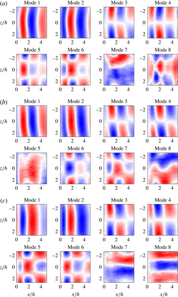
The first 8 POD modes of the fluctuating component of streamwise velocity ( $u^{\prime }$ ) in the wake at $y=1.5~\text{mm}$ for (a) $Re(h)=3500$ , (b) $Re(h)=5200$ and (c) $Re(h)=7000$ . The secondary instability wavelength is not visible in any of the modes.

Figure 13.

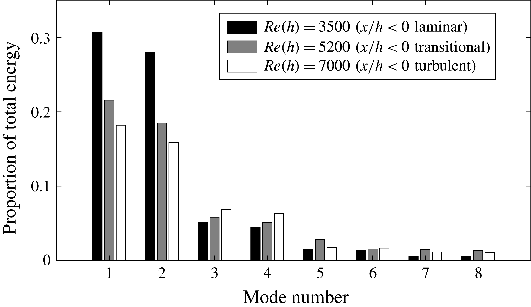
Energy associated with each of the POD modes given in figure 12. A shift in energy to the higher modes occurs as $Re$ is increased, indicating higher levels of turbulence.

The POD of $u^{\prime }$ by the method of snapshots (Sirovich Reference Sirovich1987) has been performed on the snapshots within FOV2 ( $x>0$ only, i.e. just the wake) for $Re(h)=3500$ , 5200 and 7000. The first 8 POD modes and their energy content are given in figures 12 and 13, respectively. The first two POD modes for each $Re$ capture the dynamics of the primary instability, and modes 3 and 4 capture its large-scale distortion. These first 4 POD modes contain large fractions of the energy in the flow with respect to the remaining modes as shown in figure 13. It is not clear if modes 5–8 are related to the distortion of the primary instability or the spanwise modulation of the secondary instability if $\unicode[STIX]{x1D706}_{z}$ is not known a priori. Figure 13 also reveals that the energy captured within the initial POD modes shifts to the higher modes as $Re$ increases. As it is expected, it becomes increasingly difficult to capture the complete dynamics of the flow using only a few modes when the levels of turbulence increase. Additionally, the first 8 POD modes presented here are in agreement with those given by Naghib-Lahouti et al. (Reference Naghib-Lahouti, Lavoie and Hangan2014), and 6 of the modes for each $Re$ are practically identical between studies.

The snapshots of $u^{\prime }$ have been reconstructed using varying numbers of modes and the same autocorrelation analysis used in § 3.4 to determine the distance between adjacent low-speed zones ( $\unicode[STIX]{x1D6EC}_{z}$ ) in the wake has been performed on the reduced-order ensembles. This was done to investigate the impact that the POD of $u^{\prime }$ has on the PDFs of $\unicode[STIX]{x1D6EC}_{z}$ . The effect of using 16, 24, 32 and 48 modes to reconstruct the snapshots of $u^{\prime }$ was investigated. These four cases cover the analyses of Naghib-Lahouti et al. (Reference Naghib-Lahouti, Doddipatla and Hangan2012, Reference Naghib-Lahouti, Lavoie and Hangan2014), which used either 32 POD modes or enough modes to retain at least 70 % of the energy in the flow. This energy criterion was met by using 16–32 modes depending on $Re$ in the latter case. Figure 14 displays the impact of these reconstructions on the PDFs of $\unicode[STIX]{x1D6EC}_{z}$ in the wake at $x=2h$ for $Re(h)=3500$ , 5200 and 7000. Note that a kernel technique was necessary for estimating the PDFs once the distributions became multimodal (Sheather Reference Sheather2004).

Figure 14.

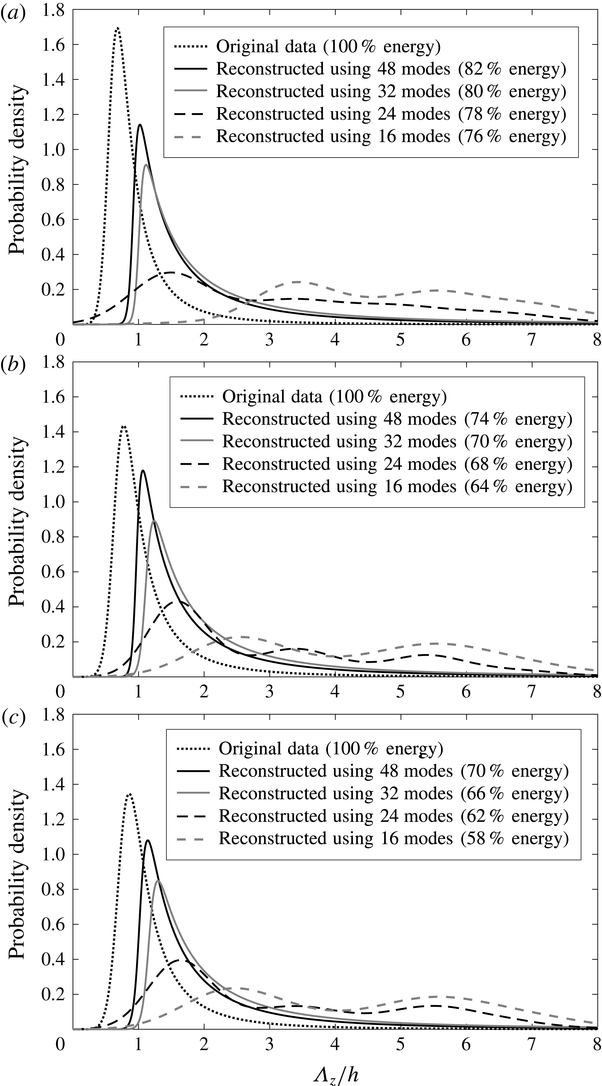
Effect of number of modes used in POD reconstruction on the probability density functions of the distances between low-speed zones ( $\unicode[STIX]{x1D6EC}_{z}$ ) in the wake at $x=2h$ for (a) $Re(h)=3500$ , (b) $Re(h)=5200$ and (c) $Re(h)=7000$ . The distributions were calculated using the same spatial autocorrelation that is covered in § 3.4. The distributions are highly sensitive to the number of POD modes used in reconstruction of the data.

The PDFs in figure 14 show that the distributions of $\unicode[STIX]{x1D6EC}_{z}$ are highly sensitive to how many modes are used to reconstruct the snapshots. In general, using fewer modes causes the peak of each distribution to decrease in magnitude and shift to the right, thus erroneously increasing the estimated values for $\unicode[STIX]{x1D706}_{z}$ . When 24 modes are used for reconstruction, the PDFs become multimodal with the first peak bearing some resemblance to the expected peak for $\unicode[STIX]{x1D706}_{z}$ . The peaks following the first one likely represent the wavelengths present in some of the more energetic modes, for example modes 3 and 6 for any $Re$ in figure 12. When 16 modes are used for reconstruction, the presence of the first distinct peak that represents $\unicode[STIX]{x1D706}_{z}$ is no longer dominant, suggesting that the majority of information regarding the secondary instability is stored beyond mode 16.

It is evident that the application of POD to streamwise–spanwise snapshots of $u^{\prime }$ when determining $\unicode[STIX]{x1D706}_{z}$ is highly dependent on the number of POD modes used to reconstruct the data ensembles and must be carefully applied. For example, when using 48 modes to reconstruct $u^{\prime }$ and thus preserving at least 70 % of the energy in the flow as was done by Naghib-Lahouti et al. (Reference Naghib-Lahouti, Lavoie and Hangan2014), the mean values for $\unicode[STIX]{x1D6EC}_{z}$ in the wake are 2.24 $h$ , 2.21 $h$ and 2.26 $h$ for $Re(h)=3500$ , 5200 and 7000, respectively. These values nearly exactly match $\unicode[STIX]{x1D706}_{z}$ for the mode B $^{\prime }$ instability predicted by Ryan et al. (Reference Ryan, Thompson and Hourigan2005) and fall within the range of mean values reported by Naghib-Lahouti et al. (Reference Naghib-Lahouti, Doddipatla and Hangan2012, Reference Naghib-Lahouti, Lavoie and Hangan2014). When the original snapshots are used (100 % energy), the mean values are 1.01 $h$ , 1.21 $h$ and 1.29 $h$ , respectively, and are consistent with the direct measurements of the secondary vortices in the present study. There are large differences in $AR$ between these studies and the present investigation, and so this does not dismiss the presence of mode B $^{\prime }$ for small $AR$ ; however, a re-evaluation of the wavelength of the secondary instability and the formation of mode B $^{\prime }$ for elongated blunt bodies with $AR$ smaller than what is considered here is suggested.