INTRODUCTION
There is currently much concern about the relationship between agriculture and climate change. Research has focused on three main topics: the impacts of climate change on agricultural production (e.g. Alcamo et al. Reference Alcamo, Dronin, Endejan, Golubev and Kirilenkoc2007; De Silva et al. Reference De Silva, Weatherhead, Knox and Rodriguez-Diaz2007; Rodriguez-Puebla et al. Reference Rodriguez-Puebla, Ayuso, Frias and Garcia-Casado2007; Wu et al. Reference Wu, Shibasaki, Yang, Tan, Matsumura and Sugimoto2007), the potential for agriculture and land use to mitigate some of the impacts of climate change (e.g. Nonhebel Reference Nonhebel, Brouwer and McCarl2006; Clifton-Brown et al. Reference Clifton-Brown, Breuer and Jones2007; Lal et al. Reference Lal, Follett, Stewart and Kimble2007; Warwick HRI Reference Warwick2007), and finally the direct contribution of agriculture to climate change (Kasimir-Klemedtsson et al. Reference Kasimir-Klemedtsson, Klemedtsson, Berglund, Martikainen, Silvola and Oenema1997; Foster et al. Reference Foster, Green, Bleda, Dewick, Evans, Flynn and Mylan2006; Vuichard et al. Reference Vuichard, Soussana, Ciais, Viovy, Ammann, Calanca, Clifton-Brown, Fuhrer, Jones and Martin2007). One aspect of this last topic is termed ‘carbon accounting’ and is concerned with estimating the total amount of greenhouse gases (GHGs) emitted during the production, processing and retailing of agricultural and food products (Carbon Trust 2007).
The final summary of the GHGs emitted during the production of a given product is termed a carbon footprint. In the present paper, the term carbon footprint is used to include emissions of the three most important GHGs emitted from agricultural activities; namely carbon dioxide (CO2), nitrous oxide (N2O) and methane (CH4). Although other GHGs such as halocarbons, ozone and carbon monoxide also contribute to climate change, they are not typically included in analyses of agricultural activities (Carbon Trust 2007).
Once carbon footprints have been estimated they may be used to inform supply chain professionals about the relative impacts of different products and activities. It is also possible to declare the carbon footprint of a product on the packaging; a so-called carbon label. The carbon label could act in a similar way to many other product labels which assume that concerned consumers will preferentially purchase goods with attributes that they value, here a low carbon footprint (Edwards-Jones et al. Reference Edwards-Jones, Milà i Canals, Hounsome, Truninger, Koerber, Hounsome, Cross, York, Hospido, Plassmann, Harris, Edwards, Day, Tomos, Cowell and Jones2008).
If the consumption patterns of consumers were influenced by carbon labels, then the producers with the lowest carbon footprint may have a commercial advantage. For this reason, a significant commercial interest in the process and outcomes of carbon labelling might be expected. Unfortunately, there are currently no agreed standards regarding the methodology for developing a carbon footprint. A standard methodology, the Publicly Available Specification (PAS) 2050, was published in the UK in late 2008 (BSI 2008). In addition, several other carbon accounting frameworks are being developed in different countries (Brenton et al. Reference Brenton, Edwards-Jones and Jensen2009); however, at the moment none of these methodologies is legally binding and, in all likelihood, further developments in climate science will provide additional stimulation of these methodologies in the future. For these reasons, and given that carbon footprinting is still a relatively new concept in agriculture, there is potential for the carbon footprints that are developed in the absence of an agreed international standard to show considerable variation in methodology and results.
The current paper utilizes data collected from two case study farms in Wales, UK, in order to calculate the carbon footprint of the lamb and beef produced. A sample of two farms cannot be representative of all production systems in a country or region, and there is no attempt to offer any average or representative values for lamb and beef production in Wales. However, it is believed that the paper is the first study to be reported in the peer-reviewed literature, which uses empirical farm-based data to calculate a carbon footprint for lamb. While these data may be of interest, the main value of the current work lies in highlighting some of the important areas, which may need to be considered by future studies.
METHODS
Carbon footprinting and life cycle assessment (LCA)
LCA has been used to analyse the environmental impacts of many products including food and agricultural products (e.g. Foster et al. Reference Foster, Green, Bleda, Dewick, Evans, Flynn and Mylan2006; Milà i Canals et al. Reference Milà i Canals, Cowell, Sim and Basson2007; Sim et al. Reference Sim, Barry, Clift and Cowell2007; Edwards-Jones et al. Reference Edwards-Jones, Plassmann, York, Hounsome, Jones and Milà i Canals2009). LCA typically considers the global warming potential of GHGs as part of its output; however, it is possible to calculate a carbon footprint without undertaking a full LCA. The methodology of LCA is standardized (ISO 2006a, b) and tends to follow set methodologies and use standard databases. While there are many similarities in approaches between LCA and carbon footprinting, they are not the same thing and as carbon footprinting methodologies develop they may diverge from the standards devised for LCA. For this reason, the approach of other authors is followed (e.g. Saunders et al. Reference Saunders, Barber and Taylor2006; Williams et al. Reference Williams, Audsley and Sandars2006) in presenting the carbon footprint independently of a full LCA.
Definition of system boundaries
Estimates of the carbon footprint of a system will depend on how the system of concern is defined. System boundaries may be defined so that they include only certain elements of the food chain. For example, those interested in farm level activities may define the system so that it only includes on-farm activities and emissions from the manufacture and delivery of inputs to the farm, but ignores processing and retail. Alternatively, it could be drawn to include other elements of the food chain, such as production, processing and retailing. When considering livestock farming and processing, at least six system boundaries can be defined. These become successively more complex and comprehensive as the system boundary is expanded, as shown below:
On-farm activities include:
1. Emissions arising from the manufacture and distribution of farm inputs (cf. embodied energy in the classic approaches to LCA, ISO 2006a, b). Also to include the use of these inputs on the farm (e.g. consider emissions related to production of fertilizer and its transport as well as direct use of fuel on farm), but ignoring the flows of GHGs into and out of animals, plants and soils that occur on farm.
2. The items in (1) above, plus the GHG emissions from livestock and their excreta as well as emissions from soils related to fertilizer use and manure management (i.e. this system boundary includes N2O emissions from nitrogen fertilizer application or manure and CH4 production from livestock and excreta).
3. The items in (2) above, but also consider the flow of GHGs into and out of soils and plants in the productive and non-productive areas of the farm, e.g. woodlands.
On-farm activities, processing, retailing and consumption include:
4. Emissions arising from the manufacture, distribution and use of farm inputs and processes up to the farm gate plus transport, processing, packaging, retailing, consumption and waste disposal.
5. The items in (4) above plus the GHG emissions from livestock, their excreta, soils and manure management.
6. The items in (5) above, but also consider the flow of GHGs into and out of soils and plants in the productive and non-productive areas of the farm, e.g. woodlands.
Non-productive areas of farms as included in boundaries 3 and 6 may form quite large areas in many agricultural systems, and these and the pastures themselves may have the potential to sequester carbon and methane (Castaldi et al. Reference Castaldi, Costantini, Cenciarelli, Ciccioli and Valentini2007; Chapuis-Lardy et al. Reference Chapuis-Lardy, Wrage, Metay, Chotte and Bernoux2007). Unfortunately, the flow of GHGs into and out of agricultural plants and soils remains relatively poorly understood, and for this reason they are ignored in the current paper. This is in accordance with the current methodological proposals of the PAS 2050 (BSI 2008).
Data collection and description of case study farms
Two case study farms were selected: firstly because they were typical of Welsh production systems, and secondly because of the availability of good records. Information on farm structure, energy use and indirect inputs for the 12 months between November 2005 and October 2006 was obtained. For both farms, the carbon footprint using system boundaries 1 and 2 as described above was calculated. The data needed to calculate energy use and GHG emissions beyond the farm gate were not available. Results are presented as kg CO2 eq/ha/year and as kg CO2 eq/kg of product based on economic allocation.
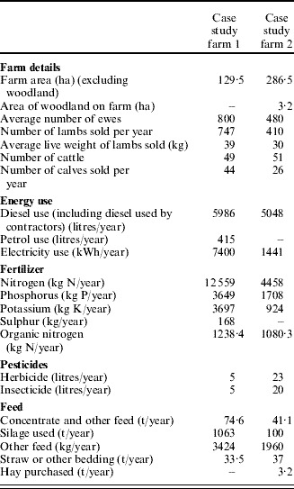
The annual inputs and outputs of the two case study farms are shown in Table 1. Both farms are mixed sheep and cattle farms. Case study farm 1 is an upland farm and a high proportion of its land is improved and fertile. The lambs are sold direct to slaughter from early July until the following January, with an average age of 6–7 months. All soils are mineral. The farm grows 4·9 ha of cereals and 8·1 ha of forage crops. Case study farm 2 is a hill farm with very little lowland. The lambs are marketed direct to slaughter from late June until November with a high proportion being sold from late summer to November. The average age is 5–6 months. About 0·75 of soils (215 ha) are organic. Both farms have a Tir Gofal agri-environmental agreement (WAG 2006) and both are ‘Hybu Cig Cymru’ (HCC; ‘Meat Promotion Wales’, a levy-funded body concerned with production and marketing of red meat in Wales) development farms.
Description of the two Welsh case study farms. Data on organic nitrogen are the means; the estimated range for farm 1 is 743–1981 kg N/year and for farm 2 is 648–1729 kg N/year

Data sources for GHG emissions for inputs and processes
In general, there were no available data on emissions associated with the manufacture and use of inputs in a Welsh context. Some data were available at UK level but, in order to collate a database of emission factors, it was necessary to utilize data from across the globe. This inevitably introduced some uncertainty into the relevance of the emission factors to the Welsh situation. It also highlighted the variation in published estimates of emission factors for many agricultural inputs. In view of both of these factors, a range of reported emissions was used throughout the calculations in order to define a minimum, maximum and mid-range value of possible emissions. Where emission factors defined by the Intergovernmental Panel on Climate Change (IPCC) were used, the uncertainty range surrounding these defaults was considered in order to reflect uncertainty in their estimation. Where data were not available from the IPCC information provided in other agriculturally related studies was used. These sources are referenced alongside the relevant information.
Emission factors for on-farm activities (system boundary 1)
Inputs
Using data presented in Tzilivakis et al. (Reference Tzilivakis, Warner, May, Lewis and Jaggard2005) for the UK, emissions from the use of diesel were calculated as 2·74 kg CO2 eq/litre of diesel. This figure includes all emissions along the supply chain and from combustion. For petrol and electricity, the DEFRA (2007) figures of 2·315 kg CO2/litre petrol and 0·523 kg CO2/kWh were used; these figures do not include N2O and CH4 emissions.
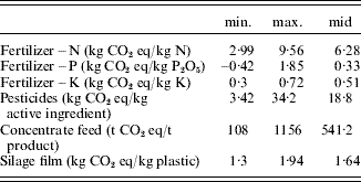
Literature values were collated for emission factors relating to the manufacture of fertilizers, pesticides and concentrate feed (Table 2). Only studies reporting all three main GHGs (CO2, N2O and CH4) were considered. Some of these figures originate from countries other than the UK, where different transportation distances and energy mixes used may result in different emission factors. Another potential problem with these data is that the figures from different studies include different processes, e.g. production, packaging, transportation, storage and transfer, with some being more comprehensive than others, and some not stating exactly which processes are included.
Ranges of GHG emissions from the production of different fertilizers, pesticides, concentrate feed and silage film reported in the literature. The negative value for P fertilizer is due to emission credits for the export of steam generated during exothermic production processes in modern plants (Wood & Cowie Reference Wood and Cowie2004)

Data on GHG emissions from phosphate fertilizer production were obtained from the literature as kg CO2 eq/kg P2O5. Data on energy use during potassium fertilizer manufacture were obtained from the literature; the only conversion factor from energy use to GHG emissions was found in Saunders et al. (Reference Saunders, Barber and Taylor2006). For sulphur, the only information available in the literature were the figures used by Saunders et al. (Reference Saunders, Barber and Taylor2006) (energy use: 5 MJ/kg; emission rate: 0·06 kg CO2/MJ). For both potassium and sulphur fertilizer, the Saunders et al. (Reference Saunders, Barber and Taylor2006) figures used were originally taken from a New Zealand study and exclude N2O and CH4. Organic nitrogen applied was calculated using IPCC methods, taking into account the number of livestock, length of time housed and manure management system used.
Silage film for silage clamps was assumed to be used for 2 years. The range for concentrate feed covers a variety of feed types, which may not accurately reflect the feed used on the case study farms. The only figure available for bedding, straw and hay were an energy use of 1·50 MJ/kg dry matter and an emission rate of 0·058 kg CO2/MJ (Saunders et al. Reference Saunders, Barber and Taylor2006); these figures were originally specified for New Zealand and may not reflect UK conditions.
Emission factors for emissions from livestock and nutrient management (system boundary 2)
Data and equations (Tier 1) from the IPCC guidelines on national GHG reporting (IPCC Reference Eggleston, Buendia, Miwa, Ngara and Tanabe2006) were used to assess the GHG emissions arising from the grazing animals and their excreta, as well as from soils following nitrogen additions as synthetic fertilizer and manure. These emission factors are default values, which may not always accurately reflect local conditions, but they were used in the current study due to a lack of locally validated figures. Emissions were calculated using these default values and their uncertainty range as minimum and maximum values. Emissions from lambs and their excreta were calculated not per year, but for the actual average time that they remained on the case study farms. Sheep stayed outside all year round; cattle were housed for 6 months per year on both case study farms. Calves were assumed to remain on the farms for 12 months.
CH4 from enteric fermentation
IPCC default emission factors suggest that each adult sheep emits 8 kg CH4/year through enteric fermentation. For lambs less than 1 year old, an emission factor of 3·2 kg CH4/year was applied as in Baggott et al. (Reference Baggott, Cardenas, Garnett, Jackson, Mobbs, Murrells, Passant, Thomson, Watterson, Adams, Dore, Downes, Goodwin, Hobson, Li, Manning, Milne, Thistlethwaite, Wagner and Walker2007) for the UK national GHG inventory. For non-dairy cattle, the IPCC default is 57 kg CH4/animal/year, which applies to adults and calves.
CH4 from excreta and manure management
Emissions of CH4 in the field and from stored cattle excreta were calculated using emission factors presented in Baggott et al. (Reference Baggott, Cardenas, Garnett, Jackson, Mobbs, Murrells, Passant, Thomson, Watterson, Adams, Dore, Downes, Goodwin, Hobson, Li, Manning, Milne, Thistlethwaite, Wagner and Walker2007) and IPCC equations. Methane emissions from manure management amount to 0·19 kg CH4/animal/year for adult sheep and 0·076 kg CH4/animal/year for lambs less than 1 year old. For adult beef cattle and cattle less than 1 year old, the values are 2·74 and 2·96 kg CH4/animal/year, respectively.
Direct and indirect N2O emissions from managed soils
Direct and indirect N2O emissions from managed soils were calculated using standard IPCC methods. An increase in available nitrogen increases nitrification and denitrification rates, resulting in increased N2O emissions. Direct N2O emissions from managed soils were calculated taking into account synthetic nitrogen fertilizers, organic fertilizers and urine and dung deposited on the pasture by livestock. Emissions from the area of managed organic soil were also included. Indirect N2O emissions from the soil to which nitrogen is applied occur through volatilization and leaching.
Direct and indirect N2O emissions from manure management
Direct emissions occurring during the storage and treatment of manure before it is applied to land were calculated according to IPCC methods. Emissions generated by excreta in the field were estimated and are reported as part of the variable ‘N2O emissions from managed soils’. Indirect emissions resulting from volatile nitrogen losses during manure collection and storage were calculated using IPCC methods. As the sheep stayed outside all year round, this calculation was only carried out for the cattle that are housed for 6 months per year on both case study farms.
Economic allocation and functional units
Both case study farms were mixed sheep and beef farms with several outputs: lamb, beef, cull ewes and wool. Based on gross income derived from these outputs, GHG emissions were allocated as follows: 0·55 to lamb, 0·35 to beef, 0·09 to cull ewes and 0·02 to wool for case study farm 1; and 0·53 to lamb, 0·36 to beef, 0·10 to cull ewes and 0·02 to wool for case study farm 2. The final product of most traditional livestock farms is live animals, which is why the results are presented per kg live weight. For lambs and cull ewes, emissions are also expressed per kg dead weight calculated using a killing out proportion for lamb of 0·45 and 0·47 for case study farm 1 and case study farm 2, respectively, and 0·30 for cull ewes for both farms. However, it is important to remember that the calculation of GHG emissions stops at the farm gate, so neither emissions from the transport of the animals to the slaughterhouse nor those related to slaughtering, butchering and retailing are included in the analysis. Only if full data are available for the supply chain up to and including the abattoir will it become more useful to use dead weight as the functional unit. The beef cattle are not fully grown when leaving the farms, as they are sold to other farmers who ‘finish’ them prior to sale. For this reason the expression of GHG emissions per kg dead weight was not considered relevant in this context.
In addition to expressing results on a per kg basis, they are also presented on a per hectare basis. This was done in order to consider the whole system as an integrated production unit and relates to the aim of reducing the environmental impacts caused by the agricultural production on a given area of land.
Some methodological issues
Emissions of GHGs associated with the manufacture and ongoing maintenance of capital goods were not included in the analysis. This was primarily due to a lack of data. However, Frischknecht et al. (Reference Frischknecht, Althaus, Bauer, Doka, Heck, Jungbluth, Kellenberger and Nemecek2007) recently evaluated the contribution of capital goods in LCA studies of agricultural products and concluded that with regard to climate change, capital goods have a minor impact and could thus be excluded. The exclusion of capital goods is also in accordance with the carbon footprint methodology proposed by the PAS 2050 (BSI 2008). Emissions from the disposal of farm waste (e.g. empty fertilizer bags, pesticide containers, silage wraps, etc.) and dead livestock were not included in calculations. Similarly, emissions related to the production of medicines such as antibiotics or vaccines were excluded from the analysis, as were emissions resulting from the visits to the farm made by vets and other business advisors. These items were excluded from this analysis due to the absence of relevant data, but ideally they would be included in the analysis. For both case study farms, all replacement livestock were assumed to be reared on the farm. All silage used was taken to have been produced on-farm. When calculating the emissions from lambs and their excreta, it was assumed that they stay on the farm for 6·5 months for case study farm 1 and 5·5 months for case study farm 2. Calves and young stock were assumed to stay on the farms for 12 months.
Case study farm 1 grows 4·9 ha of cereals and 8·1 ha of forage. Inputs could not be separated into grassland, cereals or forage, so that total farm emissions per hectare were calculated based on total farm hectares, not grassland hectares. The emissions that may arise from any potential ploughing of rotational grasslands were not taken into consideration due to the uncertainty surrounding relevant emission factors. Case study farm 2 sends 150 ewe lambs away over the winter (64 km). Emissions from sheep and their excreta were calculated as if they remained on the farm all year round, but additional concentrate feed, electricity, diesel, etc. used while the sheep were away were not included in the calculations. These additional inputs were considered to be negligible in the context of the carbon footprint of the overall farm.
For some emissions, no range of values is presented due to a lack of data in the literature. As IPCC default factors are not necessarily the mid value of their uncertainty range this means that for overall totals, the mid value given in the tables may not be the middle of the range calculated. The conversion of the different GHGs to CO2 equivalents was done using the IPCC (2001) factors of 1 for CO2, 23 for CH4 and 296 for N2O over a hundred year time horizon.
RESULTS
GHG emissions from on-farm activities (system boundary 1)
Case study farm 1
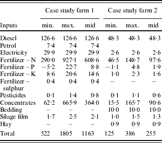
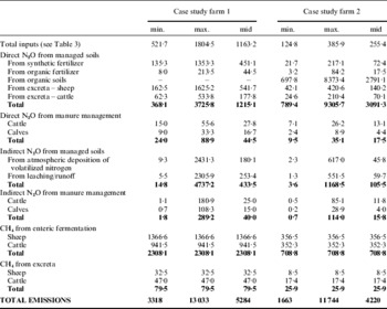
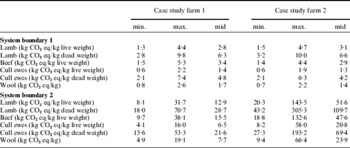
Total GHG emissions ranged from 522 to 1805 kg CO2 eq/ha/year (Table 3). Emissions were dominated by nitrogen fertilizer, followed by concentrate feed and diesel use. The lowest emissions were associated with silage film, pesticides and sulphur. GHG emissions per kg product based on economic allocation are shown in Table 5. Per kg live weight, GHG emissions for lamb were lower than for beef by 0·6 kg CO2 eq/kg.
GHG emissions in kg CO2 eq/ha/year arising from the production, delivery and use of inputs into two Welsh mixed sheep/cattle farms, calculated using a range of values reported in the literature. The minimum (min.), maximum (max.) and middle value (mid) of these ranges were used to represent the best case, worst case and average scenario. Estimation of the middle value is described in the text; for IPCC emission factors the middle value is the IPCC default value, for other emission factors it is the median. Totals have been rounded to whole numbers

Case study farm 2
Total GHG emissions ranged from 125 to 386 kg CO2 eq/ha/year (Table 3). As in case study farm 1, nitrogen fertilizer, concentrate feed and diesel use dominated emissions. The lowest emissions were associated with potassium fertilizer, pesticides and phosphate fertilizer. GHG emissions per kg live weight were similar for lamb and cattle (Table 5).
GHG emissions from on-farm activities plus emissions from livestock and nutrient management (system boundary 2)
Case study farm 1
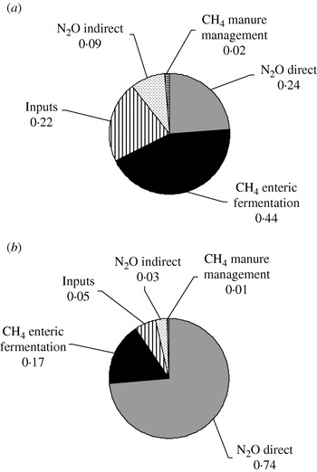
Total emissions increased substantially when GHG emissions from the grazing animals, their excreta and soils were added to the emissions arising from the farm operations (ranging from 3 to 13 t CO2 eq/ha/year) (Table 4). Emissions were dominated by CH4 from enteric fermentation, followed by direct N2O emissions from soils (Fig. 1 a). This highlights the importance of these GHGs for agricultural systems and for the results of carbon footprint studies emissions per kg product also increased considerably (Table 5). The average scenario carbon footprint for lamb was lower (13 kg CO2 eq/kg live weight) than cattle (16 kg CO2 eq/kg live weight), although the minimum to maximum ranges widely overlap.
Relative contribution (as a proportion) to total GHG emissions (kg CO2 equivalents) of farm inputs, direct and indirect N2O emissions from soil and manure management and CH4 emissions through enteric fermentation and from manure management on (a) case study farm 1 and (b) case study farm 2. Indirect emissions of N2O arise after leaching and volatilization. Figures relate to system boundary 2 (described in the text).

Total GHG emissions in kg CO2 eq/ha/year on two Welsh mixed sheep/cattle farms. Emissions from farm inputs are derived from Table 3. All emissions calculated using a range of values reported in the literature. The minimum (min.), maximum (max.) and middle value (mid) of these ranges were used to represent the best case, worst case and average scenario. Estimation of the middle value is described in the text; for IPCC emission factors the middle value is the IPCC default value, for other emission factors it is the median. Totals have been rounded to whole numbers

GHG emissions in kg CO2 equivalents per kg of product for lamb, beef, cull ewes and wool based on economic allocation. The minimum (min.), maximum (max.) and middle value (mid) of these ranges were used to represent the best case, worst case and average scenario. Estimation of the middle value is described in the text; for IPCC emission factors the middle value is the IPCC default value, for other emission factors it is the median

Case study farm 2
As with case study farm 1, the widening of the system boundary increased emissions (ranging from 2 to 12 t CO2 eq/ha/year) (Table 4). Emissions were dominated by direct N2O emissions from soils, especially from organic soils, followed by CH4 from enteric fermentation (Fig. 1 b). On this farm, the average carbon footprint of lamb was greater than cattle (52 and 48 kg CO2 eq/kg live weight, respectively; Table 5), although again the ranges largely overlap.
DISCUSSION
Limitations
The current study only presents data for two Welsh farms, representing only two Welsh farming systems. In order to develop a more robust and general picture of the carbon footprint of Welsh sheep and beef farming, a greater number of farms and farm types would need to be investigated. For example, the footprint of an intensive lowland farm is likely to differ considerably from the very extensive upland farm in case study farm 2. Another factor to be considered when interpreting results is that both case study farms are formally involved in technology transfer schemes, which require them to demonstrate and promote the principles of business development, environmental safeguarding and market focus. They implement management changes and new technologies designed to improve gross margins as well as sustainability. In addition, both farms have agri-environment agreements, which involve setting maximum stocking rates on semi-natural habitats. This means that the case study farms may implement best practice and environmentally friendly practices, which may not be universally practiced on Welsh sheep farms. For this reason, the results may not be representative of the average Welsh production system. Also it is important to note that the real-farm data used in the calculations here represent one particular year. Farm practices, inputs and outputs may vary between years according to climatic conditions and extreme events, and longer term data would help gain clearer insight into the real carbon footprint of lamb production.
Comparison with other studies
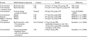
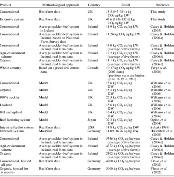
The emissions per kg of live weight reported here for lamb on the two case study farms (8·1–31·7 and 20·3–143·5 kg CO2 eq/kg live weight) overlap with most of the other published data on this topic (Table 6). Similarly for beef, the current range of data (9·7–38·1 and 18·8–132·6 kg CO2 eq/kg live weight) is in broad accordance with data reported elsewhere (Table 7). Case study farm 2 has a much greater carbon footprint than case study farm 1 which is due to emissions from managed organic soils; these appear not to be included in other published studies. Unfortunately, it is difficult to make direct comparisons with previous studies as there are significant methodological differences between studies. For example, some of the carbon footprints are derived from models of relevant enterprises (e.g. Williams Reference Williams, Audsley and Sandars2006), while others utilize different system boundaries and do not consider all GHGs emitted from the system (e.g. Saunders et al. Reference Saunders, Barber and Taylor2006). The current worst case scenario has a far greater carbon footprint per kg meat than most other published studies. It is impossible to comment on the relevance of this because no other study shows an uncertainty range using ranges of reported emission factors. Casey & Holden (Reference Casey and Holden2006b) calculated ranges of emissions to assess the possible error associated with their results per functional unit, but the results ranges are smaller and the worst case scenario figure is much lower than in the present study. The results of the current study on a per hectare basis overlap with per hectare figures reported elsewhere, but again the worst case scenario has much greater values than other published studies (Table 7).
Methodological approach and carbon footprint results for sheep reported in published studies. DW, dead weight; LW, live weight. Note that studies expressing results per kg DW do not include emissions beyond the farm gate. Direct comparisons between the results of the different studies are difficult due to potentially large differences in the analytical methodologies and system boundaries adopted

Methodological approach and carbon footprint results for beef reported in published studies. DW, dead weight; LW, live weight. Note that studies expressing results per kg DW do not include emissions beyond the farm gate. Direct comparisons between the results of the different studies are difficult due to potentially large differences in the analytical methodologies and system boundaries adopted

The current experience of analysing empirical data collected directly from farms (present study and Edwards-Jones et al. Reference Edwards-Jones, Plassmann, York, Hounsome, Jones and Milà i Canals2009) suggest that the realities of estimating carbon footprints of farm systems are far more complicated than is normally expressed in models of agricultural enterprises. These complexities relate to the mixture of interacting enterprises on farms, which may utilize shared resources, and also to the range of on-farm management systems which do not easily map on to any of the IPCC categories, e.g. manure handling systems. These issues render the identification of relevant emission factors a difficult, and ultimately subjective, process. Similarly physical differences between locations, farming systems and the skill of farmers themselves introduce significant variation into the system. As such, analyses of regional averages may not necessarily offer useful representations of all of a region's farm systems. The large difference in emissions of nitrous oxide between case study farm 1, which is on mineral soils, and case study farm 2, which is on organic soils, is a good example of such differences.
These issues are exacerbated by the variation in relevant emissions data that are available in the literature (e.g. for fertilizers). By explicitly utilizing this range in current calculations it was possible to calculate the minimum and maximum carbon footprint for the systems analysed. This is a relatively novel approach, as most studies simply report a single figure. Indeed even LCAs tend to report single values (but see Milà i Canals et al. (Reference Milà i Canals, Cowell, Sim and Basson2007) for an example of a study which does report variation), and the treatment of uncertainty in LCA is an active source of discussion within the discipline. This variation suggests that if analysts adopted a similar accounting framework when estimating carbon footprints, the judicious use of emission factors could result in very different results being produced for the same product. As a result both the explicit strategic behaviour of experienced analysts, and the naïve use of data by less experienced analysts, may result in large differences in the carbon footprints of similar products. Should such information be utilized in some commercial way, i.e. on a label or in more generic marketing campaigns, then there may be potentially serious implications for producers, consumers and others in the food chain.
Functional unit
Standard LCA expresses environmental impacts for a defined functional unit, e.g. per kg of meat or litre of milk. This assumption works well for simple industrial products which are produced by a standard method. However, difficulties arise when the same process produces more than one product, and/or when these products make differential use of common resources. This is exactly the situation in the livestock systems studied in the current paper, where an animal is sold as a single unit, and the different parts of that animal can go for many different uses (e.g. wool, skins, prime cuts of meat, secondary cuts of meat and offal). A possible solution in this situation is to define the variety of products very precisely and then allocate the environmental burdens between them according to their economic value. However, in order to be able to calculate the carbon footprint per kg dead weight of the livestock, the full cooperation of the abattoirs who receive the animals would be required, and maybe also additional actors in the food chain. Although it was attempted to elicit the help of these actors in the current study, this was ultimately unsuccessful, and so it was necessary to limit the system boundary to the farm gate. Given this boundary, it is believed that the whole animal is the appropriate functional unit when considering systems that stop at the farm gate and that the functional unit to express the carbon footprint up to the farm gate should be kg live weight. While this approach may be at odds with much practice in LCAs of food products until now, it seems to be a sensible approach to the situation where empirical data are not available beyond the farm gate. Further studies may be able to gain such data and thereby enhance our understanding of appropriate allocations of environmental burdens.
In addition to expressing the carbon footprint of these farming systems per kg live weight, it is believed a more complete description of the farm system can be gained by considering the output of GHGs per hectare of land alongside that of the products. Such data provide an insight into the intensity of land use, and enable a more complete assessment of the whole farming system.
Future research and methodological issues
When any future analyses of the carbon footprints of farm processes are conducted it is essential that a sufficient number of farms are sampled in order to both represent the variation in environment and farm systems, but also the variation between farms utilizing similar systems. For example, recent work by Hospido et al. (Reference Hospido, Milà i Canals, McLaren, Clift, Truninger and Edwards-Jones2009) shows that the variation in environmental burdens between farms in the same country can be as large as that between countries. Data presented in the current study were obtained from only two farms. This is clearly insufficient to enable any generalizations about Welsh production overall, but it does demonstrate the variation in the carbon footprints of lamb production systems. Given the absence of previous studies of this type it is impossible to predict the sample size needed to obtain adequate representation of the entire sector in Wales.
The current analysis has ignored the flows of GHGs into plants and soils on farms (on-farm sequestration). These items were omitted from the analysis due to the uncertainty that surrounds their quantification. However, a full system analysis of GHGs in agricultural systems would consider these stock and flows (Edwards-Jones et al. Reference Edwards-Jones, Milà i Canals, Hounsome, Truninger, Koerber, Hounsome, Cross, York, Hospido, Plassmann, Harris, Edwards, Day, Tomos, Cowell and Jones2008).
Using ranges of published emission factors during the calculation of the carbon footprint highlighted the variability of current estimates for many of the inputs used and emissions from soils and manure management. Usually, studies only consider one emission factor in their analyses, e.g. the emission factor contained in an underlying database when using LCA software. The current approach clearly indicates the level of uncertainty that is associated with carbon footprint calculations and emphasizes the need for standardization not only of methodology but also relevant emission factors to enable comparison between different studies. It also illustrates that single figures given as the result of carbon footprint calculations can be misleading by masking the uncertainties associated with underlying calculations.
It is noteworthy that case study farm 2, which has an extensive production system, appears to have a very high carbon footprint per kg of lamb produced. Most of the emissions arise from the organic soil, and are outside the control of the farmer. In addition this farm has adopted much of the environmental advice given to farmers over the last 25 years. The low stocking rate is perhaps the most obvious indicator of this. However, when viewed from the perspective of a carbon footprint this low stocking rate relates to low production efficiency, which then delivers high GHG emissions per functional unit. This highlights the potential conflict between carbon efficiencies and other environmental objectives. Further work is needed to identify systems which can produce food in a carbon efficient manner, while simultaneously maintaining other elements of the environment.
The results of the current work, and other studies, only consider a small part of the complete food system. There is an urgent need for empirical studies that cover the complete food system from production to waste disposal, and consider the emissions to and from natural parts of the ecosystem such as plants and soils. Only by taking such a holistic analysis can a thorough understanding of the impacts of food production systems on the climate be obtained.
CONCLUSION
The comparison of the results of the current study with other published carbon footprints demonstrates the variation that occurs between farms producing the same product. This insight undermines the generalizability of any carbon footprint claims made for a whole country or region which are not based on a representative sample of farms. Only through collecting data from an adequate number of similar farms within a region can the variation in their carbon footprints be understood. Even if adequate data were collected for any given enterprise, meaningful comparisons with the results of other studies can only be made if both studies adopt similar system boundaries and utilize similar emission data. To date there are too few studies of lamb to enable any such comparisons.
We are grateful for funding from Hybu Cig Cymru and for the cooperation of the case study farmers. This analysis also benefited from a parallel project funded by the UK Research Councils Rural Economy and Land Use Programme entitled ‘Comparative assessment of environmental, community and nutritional impacts of consuming fruit and vegetable produced locally and overseas’ (RES-224-25-0044).