Introduction
Suppression of high-frequency unwanted signals is one of the microstrip lowpass filter's (LPF's) applications in microwave system [Reference Hong and Lancaster1–Reference Dou, Wang, Cui and Li4]. In [Reference Alyahya, Aseeri, Bukhari, Shaman, Alhamrani and Affandi5], by using shunt stepped-impedance resonators and single-base suppressor in the center of the transmission line, an LPF has been designed. This filter has a flat passband and a stopband with proper suppression level, but it suffers from a gradual response and narrow stopband. In [Reference Zhang, Liu, Zhao, Du, Zhang and Xu6], an LPF has been designed with a hairpin stepped impedance resonator and a hexagon stub that has a wide stopband. However, the filter has a low suppression level. Using several radial structures, an LPF with a high relative stopband bandwidth (RSB) rate has been proposed in [Reference Jiang and Xu7]. This filter has an ultra-wide stopband bandwidth and a flat passband, but it suffers from large circuit size.
In [Reference Majidifar8], by using the H-shaped structure as well as the application of the spiral-defected-ground structure technique, an attempt has been made to improve responses while presenting a novel design. This LPF suffers from a gradual response in its transition band. In some papers, the cut-off frequency is significantly larger than other references, and these filters have their own specific applications. In [Reference Hayati, Naderi and Jafari9], using radial resonators and providing a simple design, an LPF with a sharp response and 4.24 GHz cut-off frequency has been designed. The flat and low lost passband is one of the prominent features of the LPF, but the RSB rate is 1.26, which is much lower than recent works. In [Reference Wang, Ge, Guo and Wu10], an LPF with a triangular patch resonator is proposed. This LPF has a cut-off frequency of 1.5 GHz and proper bandwidth. Other benefits of the presented paper in [Reference Wang, Ge, Guo and Wu10] are its sharp response with a roll-off rate of 257 dB/GHz. The normalized circuit size (NCS) rate is 0.0156(λg)2, which is one of the weak points. In [Reference Li, Qu and Xue11], a microstrip LPF using a resonator with slow-wave effects to obtain sharp skirt performance is designed. However, the size of the filter is relatively large. In [Reference Hayati, Zarghami and Kazemi12], using a resonator and a rectangular suppressing cell, as well as applying the radial structure on the edges, an LPF is designed with the figure of merit (FOM) of 173 127. In this paper, in addition to size reduction, the cut-off frequency is reduced to 1.01 GHz, which results in an improvement in the NCS rate to 0.0040 (λg)2. This benchmark is several times smaller than the presented LPF in reference [Reference Hayati, Zarghami and Kazemi12]. The previously reported works have several disadvantages such as a low suppression level, a gradual response, and a narrow stopband bandwidth. Therefore, in this paper, a compact size LPF with a simple structure using a resonator with rectangular geometry is proposed to cover these defects.
Filter design
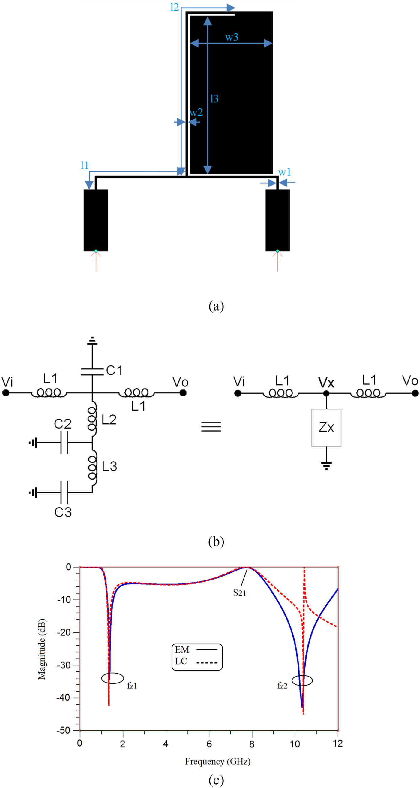
The original structure of the resonator is rectangular with long legs. The increment in height of the base of the resonator results in the increment of roll-off rate and decrement of the cut-off frequency. The increase in bandwidth is another result of the above changes. The main resonator creates a zero near the passband that causes severe resonance in this region and in fact, creates the transition band. Also, the dimensions of the main resonator and how it is placed in the filter structure are directly related to the sharpness of the response and cut-off frequency. In Figs 1(a)–1(c), the proposed resonator, its equivalent LC circuit, and frequency response are shown, respectively. The dimensions of Fig. 1(a) are as follows (all in millimeters): W1 = 0.1, W2 = 0.1, W3 = 4.05, l1 = 5.28, l2 = 10.44, l3 = 7.73.
(a) Proposed resonator. (b) Equivalent LC circuit. (c) EM and LC equivalent circuit simulation results.

Each microstrip line in the LC model is equivalent to a series inductor and a capacitor, whose end is connected to the ground. If the microstrip line is narrow and long, the value of the inductor is larger and the capacitor's value becomes smaller. According to Fig. 1, L1 and C1 are equivalent lumped components of the transmission line with the length of l1 and width of w1. Also, L2 and C2 are equivalent lumped components of the transmission line with the length of l2 and width of w2. The open-circuit stub with the length of l3 and width of w3 is equivalent to the lumped components of L3 and C3. Using equations (1)–(4), the LC equivalent circuit of the proposed resonator is calculated as follows [Reference Hong and Lancaster1, Reference Majidifar8]:
L1 = 3.5, L2 = 8.54, L3 = 0.675, C1 = 0.2725, C2 = 0.5464, C3 = 1.053 (all sizes are in nH and pF):
 $$\eqalign{C &= \Big[ 8.85{\lpar {10} \rpar }^{-12} \Big\{ {\left[ {\displaystyle{{\varepsilon r \times w} \over h}} \right]}^{1.08} \cr & \quad+ {\left[ {2\pi \left( {\displaystyle{{\varepsilon r + 1} \over 2}} \right)\left( {\displaystyle{1 \over {{\rm ln}\lpar {8h/w + 1} \rpar }}-\displaystyle{w \over {8h}}} \right)} \right]}^{1.08} \Big\}^{0.926} \Big] \times l,}$$
 $$L = \displaystyle{{Z_c \times l} \over {V_p}},\,\,\; \; \; v_p = \; \displaystyle{c \over {\sqrt {\varepsilon _{re}}}}. $$
For w/h ≤ 1:
 $$\eqalign{ \varepsilon _{re} & = \displaystyle{{\varepsilon r + 1} \over 2} + \displaystyle{{\varepsilon r-1} \over 2}\left\{ {{\left[ {1 + 12\displaystyle{h \over w}} \right]}^{-0.5} + 0.04{\left[ {1-\displaystyle{w \over h}} \right]}^2} \right\},\; \cr & Z_c = \displaystyle{\eta \over {2\pi \sqrt {\varepsilon _{re}}}} {\rm ln}\left[ {8\displaystyle{h \over w} + 0.25\displaystyle{w \over h}} \right].} $$
For w/h ≥ 1:
 $$\eqalign{\varepsilon _{re} & = \displaystyle{{\varepsilon r + 1} \over 2} + \displaystyle{{\varepsilon r-1} \over 2}\left\{ {{\left[ {1 + 12\displaystyle{h \over w}} \right]}^{-0.5},\;} \right. \cr & Z_c = \displaystyle{\eta \over {\sqrt {\varepsilon _{re}}}} \left\{ {\displaystyle{h \over w} + 1.393 + 0.677{\rm ln}\left[ {\displaystyle{w \over h} + 1.444} \right]} \right\}^{-1},} $$
where Z c and v p are the characteristic impedance and the phase velocity of the transmission line, respectively. Also, l, w, and h are the line lengths, line widths, and substrate thickness, respectively; c indicates the light speed and η is a constant equal to 377(120π) Ω [Reference Hong and Lancaster1].
With 50 Ω impedance matching in the output, V x can be written in term of V o as:
 $$\displaystyle{{V_x} \over {L1 \times S + 50}} = \displaystyle{{V_o} \over {50}},\,$$
 $$\,V_x{\rm \;} = {\rm \;} \displaystyle{{\lpar {L1 \times S + 50} \rpar V_o} \over {50}}.$$
On the other hand, we write a Kcl in the V x node:
 $$\displaystyle{{V_x-V_i} \over {L1 \times S}} + \displaystyle{{V_x} \over {Z_x}} + \displaystyle{{V_x-V_o} \over {L1 \times S}} = 0,$$
where Zx is the inductive and capacitive resistance of the Vx node and it is defined as follows:
 $$Z_x{\rm \;} = {\rm \;} \left( {\left( {\left( {\left( {\displaystyle{1 \over {C3 \times S}} + L3 \times S} \right){\rm \;} \vert \vert {\rm \;} \displaystyle{1 \over {C2 \times S}}} \right) + {\rm \;} L2 \times S} \right){\rm \;} \vert \vert {\rm \;} \displaystyle{1 \over {C1 \times S}}} \right).$$
The V o/V i ratio can be obtained by combining equations (6) and (7), as follows:
 $$\displaystyle{{V_o} \over {V_i}} = \displaystyle{{50 \times Z_x} \over {\lpar {L1 \times S + 2 \times Z_x} \rpar \lpar {50 + L1 \times S} \rpar -\lpar {50 \times Z_x} \rpar }}.$$
To find the zeros, we can obtain the f z value in terms of the inductor and the capacitors used in the circuit as follows:
 $$f_{z1} = \displaystyle{{\sqrt {\displaystyle{1 \over {C2L2}} + \displaystyle{1 \over {C2L3}} + \displaystyle{1 \over {C3L3}} + \displaystyle{{\sqrt {-4C2C3L2L3 + {\lpar {C2L2 + C3L2 + C3L3} \rpar }^2}} \over {C2C3L2L3}}}} \over {2\pi \sqrt 2}}, $$
 $$f_{z2} = \displaystyle{{\sqrt {\displaystyle{1 \over {C2L2}} + \displaystyle{1 \over {C2L3}} + \displaystyle{1 \over {C3L3}}-\displaystyle{{\sqrt {-4C2C3L2L3 + {\lpar {C2L2 + C3L2 + C3L3} \rpar }^2}} \over {C2C3L2L3}}}} \over {2\pi \sqrt 2}}. $$
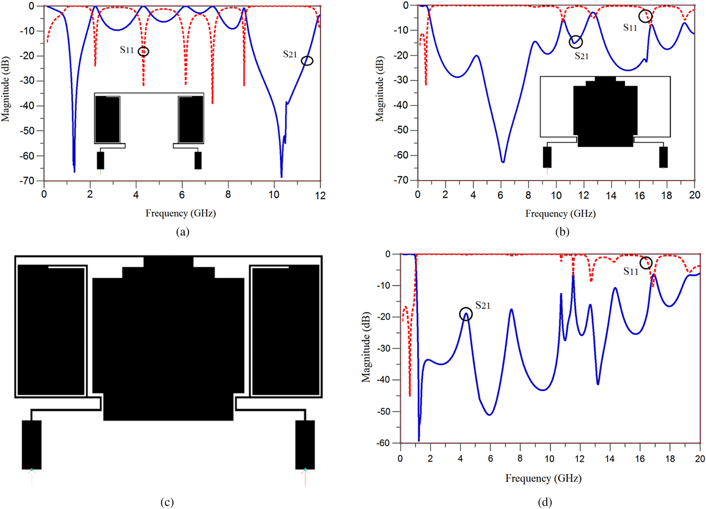
By substituting the values of inductors and capacitors in equations (10) and (11), the f z1 and f z2 are obtained as 1.338 and 10.45 GHz, respectively, which matches with simulation result as shown in Fig. 1(c). In fact, another resonator similar to the resonator shown in Fig. 1(a) is added in a symmetrical form in order to create a proper passband and a sharper response as shown in Fig. 2(a). To eliminate the unwanted harmonics from 2 to 10 GHz, a suppressing cell is added as shown in Fig. 2(b). The proposed resonators are combined with the suppressing cell as shown in Figs 2(c) and its frequency response is shown in Fig. 2(d).
(a) Resonators and their frequency responses. (b) The structure of the suppressor cell and its frequency responses. (c) The structure of the proposed filter. (d) The frequency response of the proposed filter.
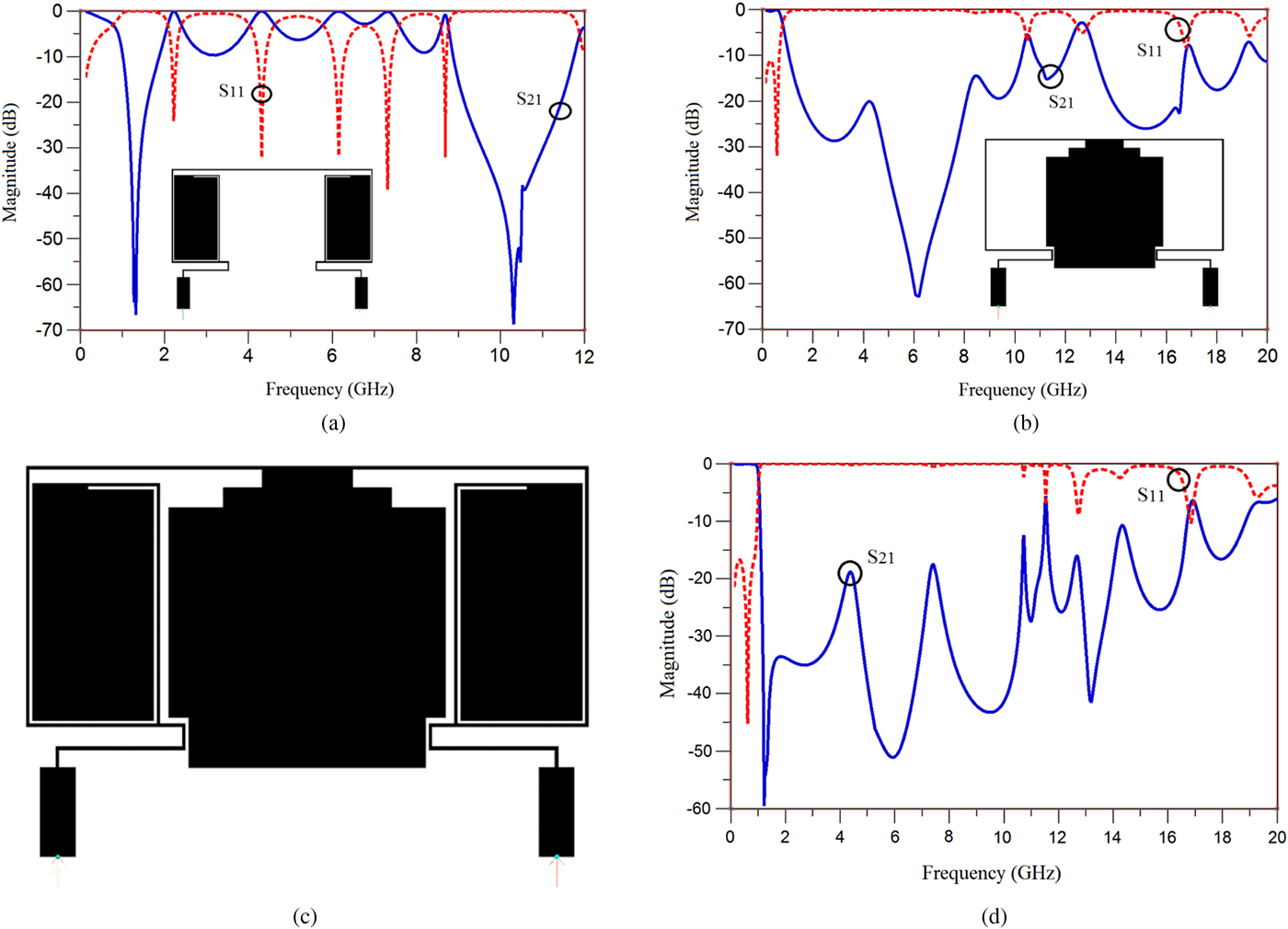
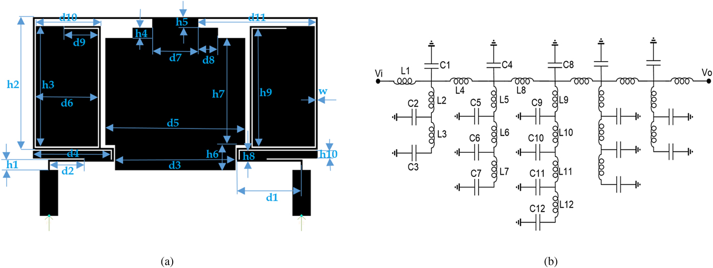
As can be observed from Fig. 2(d), the passband shows a flat response and the transition band is sharp, but the bandwidth is not good enough. To increase the bandwidth, two stubs are added as shown in Fig. 3(a), where the overall dimensions of the filter are not increased and an acceptable performance is achieved.
(a) The proposed filter. (b) Its LC model.
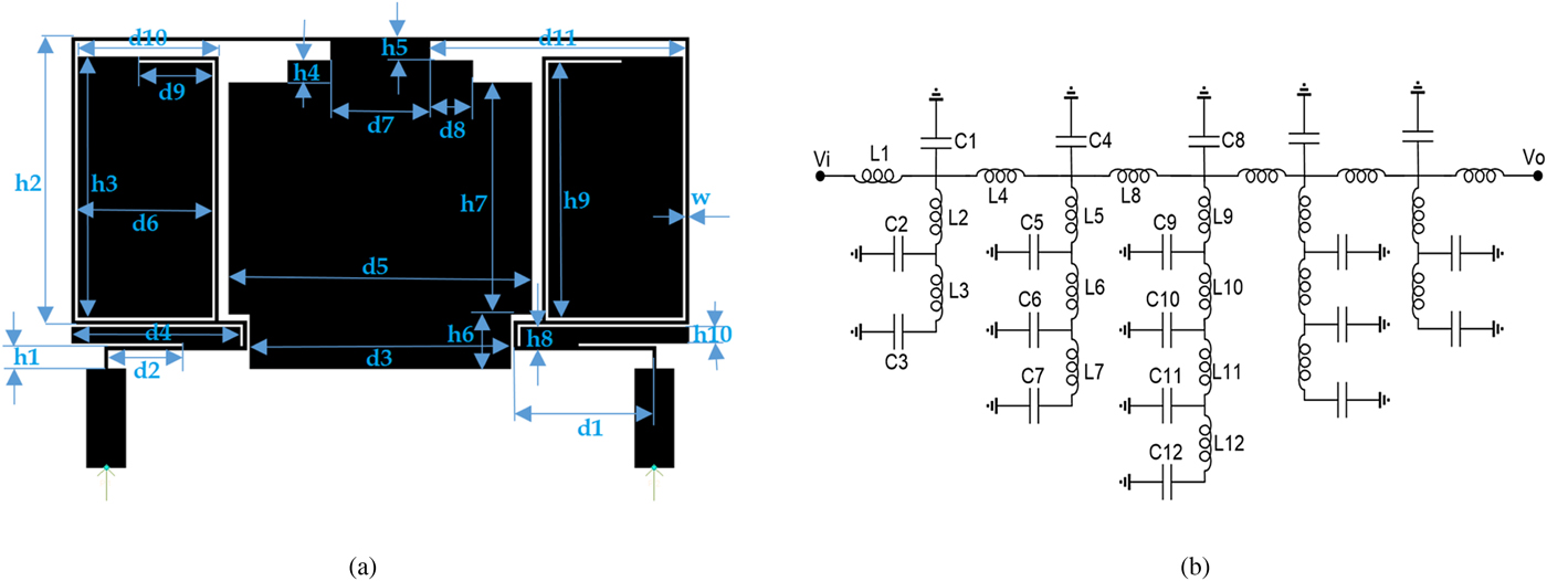
The dimensions of Figs 3(a) and 3(b) are given in Tables 1 and 2, respectively.
The dimensions of the proposed filter (all dimensions are in millimeters)

The values of each inductor and capacitor

By reducing the size of the LPF, the cut-off frequency is increased. The overall dimension of the proposed filter is 10.07 mm × 18.7 mm. In Fig. 3(b), an equivalent LC circuit is proposed for the final structure of the proposed filter. The transfer function of the circuit is shown in Fig. 3(b), as V o/V i ratio helps us to find the circuit's zeros.
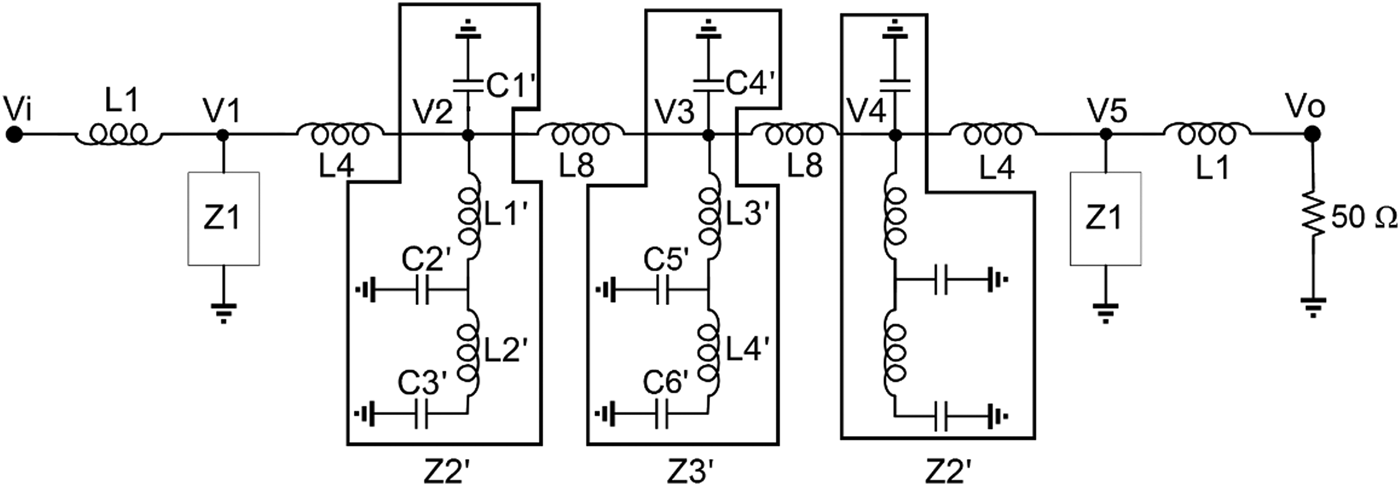
To obtain V o/V i, the nodes are named as V k where k = 1, 2, 3, 4, 5, as shown in Fig. 4 and the impedance seen from the node V k is called Z k. In order to calculate the V o/V i ratio, the following process is followed:
 $$\displaystyle{{V_o} \over {V_i}} = \displaystyle{{V_o} \over {V5}} \times \displaystyle{{V5} \over {V4}} \times \displaystyle{{V4} \over {V3}} \times \displaystyle{{V3} \over {V2}} \times \displaystyle{{V2} \over {V1}} \times \displaystyle{{V1} \over {V_i}},$$
where Z1, Z2, and Z3 values are defined as follows:
 $$Z1{\rm \;} = {\rm \;} \left( {\left( {\left( {\left( {\displaystyle{1 \over {C3 \times S}} + L3 \times S} \right){\rm \;} \vert \vert {\rm \;} \displaystyle{1 \over {C2 \times S}}} \right) + {\rm \;} L2 \times S} \right){\rm \;} \vert \vert \; \displaystyle{1 \over {C1 \times S}}} \right),$$
 $$Z2{\rm \;} = {\rm \;} \left( {\left( {\left( {\left( {\left( {\left( {\displaystyle{1 \over {C7 \times S}} + L7 \times S} \right){\rm \;} \vert \vert {\rm \;} \displaystyle{1 \over {C6 \times S}}} \right) + {\rm \;} L6 \times S} \right){\rm \;} \vert \vert \; \displaystyle{1 \over {C5 \times S}}} \right) + {\rm \;} L5 \times S} \right){\rm \;} \vert \vert {\rm \;} \displaystyle{1 \over {C4 \times S}}} \right),$$
 $$Z3{\rm \;} = {\rm \;} \left( {\left( {\left( {\left( {\left( {\left( {\left( {\left( {\displaystyle{1 \over {C12 \times S}} + L12 \times S} \right){\rm \;} \vert \vert {\rm \;} \displaystyle{1 \over {C11 \times S}}} \right) + {\rm \;} L11 \times S} \right){\rm \;} \vert \vert {\rm \;} \displaystyle{1 \over {C10 \times S}}} \right) + L10 \times S} \right){\rm \;} \vert \vert {\rm \;\;} \displaystyle{1 \over {C9 \times S}}} \right){\rm \;} + {\rm \;} L9 \times S} \right){\rm \;} \vert \vert \displaystyle{1 \over {C8 \times S}}} \right).$$
Auxiliary LC equivalent circuit to find the transfer function.

To calculate the V o/V5 ratio in the V o node, a Kcl at the output node results:
 $$\displaystyle{{V_o} \over {50}} + \displaystyle{{V_o-V5} \over {L1 \times S}} = 0,$$
 $$\displaystyle{{V_o} \over {V5}} = \displaystyle{{50} \over {L1 \times S + 50}} = A.$$
 $$V_o = A \times V5$$
Writing a Kcl for the V5 node as follows:
 $$\displaystyle{{V5} \over {Z1}} + \displaystyle{{V5-V_o} \over {L1 \times S}} = \displaystyle{{V4-V5} \over {L4 \times S}},$$
and combining equations (18) and (19), the V5/V4 ratio is obtained as:
 $$\eqalign{\displaystyle{{V5} \over {V4}} & = \displaystyle{{L1 \times Z1} \over {L1 \times L4 \times S + L4 \times Z1 + L1 \times Z1-A \times L4 \times Z1}} \cr & = B,}$$
 $$V5 = B \times V4.$$
With a Kcl in the V4 node:
 $$\displaystyle{{V4} \over {Z2}} + \displaystyle{{V4-V5} \over {L4 \times S}} = \displaystyle{{V3-V4} \over {L8 \times S}},$$
and combining equations (21) and (22), the V4/V3 ratio is obtained as:
 $$\eqalign{\displaystyle{{V4} \over {V3}} & = \displaystyle{{L4 \times Z2} \over {L4 \times L8 \times S + L8 \times Z2 + L4 \times Z2-B \times L8 \times Z2}} \cr & = C,}$$
 $$V4 = C \times V3.$$
With a Kcl in node V3, we have:
 $$\displaystyle{{V3} \over {Z3}} + \displaystyle{{V3-V4} \over {L8 \times S}} = \displaystyle{{V2-V3} \over {L8 \times S}},$$
and combining equations (24) and (25), the V3/V2 ratio is obtained as:
 $$\displaystyle{{V3} \over {V2}} = \displaystyle{{Z3} \over {2 \times Z3-C \times Z3 + L8 \times S}} = D,$$
 $$V3 = D \times V2.$$
With a Kcl in node V2:
 $$\displaystyle{{V2} \over {Z2}} + \displaystyle{{V2-V3} \over {L8 \times S}} = \displaystyle{{V1-V2} \over {L4 \times S}},$$
and combining equations (27) and (28), the V2/V1 ratio is obtained as:
 $$\displaystyle{{V2} \over {V1}} = \displaystyle{{L8 \times Z2} \over {L4 \times L8 \times S + L8 \times Z2 + L4 \times Z2-D \times L4 \times Z2}} = E,$$
 $$V2 = E \times V1.$$
Finally, with a Kcl in the V1 node:
 $$\displaystyle{{V1} \over {Z1}} + \displaystyle{{V1-V2} \over {L4 \times S}} = \displaystyle{{V_i-V1} \over {L1 \times S}},$$
and combining equations (30) and (31), the V1/V i ratio is obtained as follows:
 $$\eqalign{\displaystyle{{V1} \over {V_i}} & = \displaystyle{{L4 \times Z1} \over {L1 \times L4 \times S + L4 \times Z1 + L1 \times Z1-E \times L1 \times Z1}} \cr & = F.}$$
Now, by combining equations (12), (17), (20), (23), (26), (29), and (32), the total-circuit transform function is obtained:
 $$\displaystyle{{V_o} \over {V_i}} = A \times B \times C \times D \times E \times F.$$
Now, to find the circuit zeros, equation (33) should be equal to zero. According to equation (17), the value of A cannot be zero. A comparison between equations (20) and (32) as well as (23) and (29) shows that they are having similar zero values.
However, variable D has a different zero value. The zeros of B and F are obtained as follows:
 $$f_{z3} = \displaystyle{{\sqrt {\displaystyle{1 \over {C2L2}} + \displaystyle{1 \over {C2L3}} + \displaystyle{1 \over {C3L3}} + \displaystyle{{\sqrt {-4C2C3L2L3 + {\lpar {C2L2 + C3L2 + C3L3} \rpar }^2}} \over {C2C3L2L3}}}} \over {2\pi \sqrt 2}}, $$
 $$f_{z4} = \displaystyle{{\sqrt {\displaystyle{1 \over {C2L2}} + \displaystyle{1 \over {C2L3}} + \displaystyle{1 \over {C3L3}}-\displaystyle{{\sqrt {-4C2C3L2L3 + {(C2L2 + C3L2 + C3L3)}^2}} \over {C2C3L2L3}}}} \over {2\pi \sqrt 2}}. $$
The exact value of the resonant frequencies f z3 and f z4 is obtained with substituting values of inductors and capacitors. To find zeroes for C, E, and D, with eliminating the inductors and capacitors that have less impact on the responses, equations (14) and (15) are approximated as:
 $$Z2^{\prime}{\rm \;} = {\rm \;} (\left( {\left( {\left( {\displaystyle{1 \over {C3^{\prime} \times S}} + L2^{\prime} \times S} \right){\rm \;} \vert \vert \; {\rm \;} \displaystyle{1 \over {C2^{\prime} \times S}}{\rm \;} + {\rm \;} L1^{\prime} \times S} \right){\rm \;} \vert \vert {\rm \;} \left( {\displaystyle{1 \over {C1^{\prime} \times S}}} \right)} \right),$$
 $$Z3^{\prime}{\rm \;} = {\rm \;} (\left( {\left( {\left( {\displaystyle{1 \over {C6^{\prime} \times S}} + L4^{\prime} \times S} \right){\rm \;} \vert \vert {\rm \;} \displaystyle{1 \over {C5^{\prime} \times S}}{\rm \;} + {\rm \;} L3^{\prime} \times S} \right){\rm \;} \vert \vert {\rm \;} \left( {\displaystyle{1 \over {C4^{\prime} \times S}}} \right)} \right).$$
The simplified LC equivalent circuit is shown in Fig. 5. The quantities of inductors and capacitors forming Z2′ and Z3′ are as follows:
C1′ = 0.315, C2′ = 0.355, C3′ = 0.918, C4′ = 0.9, C5′ = 2.5, C6′ = 3.5, L1′ = 12.5, L2′ = 0.57, L3′ = 0.9, L4′ = 0.1.
Simplified LC equivalent circuit.

As a result, we have common zeroes for C and E:
 $$f_{z5} = \displaystyle{{\sqrt {\displaystyle{1 \over {C2^{\prime}L1^{\prime}}} + \displaystyle{1 \over {C2^{\prime}L2^{\prime}}} + \displaystyle{1 \over {C3^{\prime}L2^{\prime}}} + \displaystyle{{\sqrt {-4C2^{\prime}C3^{\prime}L1^{\prime}L2^{\prime} + {\lpar {C2^{\prime}L1^{\prime} + C3^{\prime}L1^{\prime} + C3^{\prime}L2^{\prime}} \rpar }^2}} \over {C2^{\prime}C3^{\prime}L1^{\prime}L2^{\prime}}}}} \over {2\pi \sqrt 2}}, $$
 $$f_{z6} = \displaystyle{{\sqrt {\displaystyle{1 \over {C2^{\prime}L1^{\prime}}} + \displaystyle{1 \over {C2^{\prime}L2^{\prime}}} + \displaystyle{1 \over {C3^{\prime}L2^{\prime}}}-\displaystyle{{\sqrt {-4C2^{\prime}C3^{\prime}L1^{\prime}L2^{\prime} + {(C2^{\prime}L1^{\prime} + C3^{\prime}L1^{\prime} + C3^{\prime}L2^{\prime})}^2}} \over {C2^{\prime}C3^{\prime}L1^{\prime}L2^{\prime}}}}} \over {2\pi \sqrt 2}}. $$
Finally, the zeros associated with D are as follows:
 $$f_{z7} = \displaystyle{{\sqrt {\displaystyle{1 \over {C5^{\prime}L3^{\prime}}} + \displaystyle{1 \over {C5^{\prime}L4^{\prime}}} + \displaystyle{1 \over {C6^{\prime}L4^{\prime}}} + \displaystyle{{\sqrt {-4C5^{\prime}C6^{\prime}L3^{\prime}L4^{\prime} + {(C5^{\prime}L3^{\prime} + C6^{\prime}L3^{\prime} + C6^{\prime}L4^{\prime})}^2}} \over {C5^{\prime}C6^{\prime}L3^{\prime}L4^{\prime}}}}} \over {2\pi \sqrt 2}}, $$
 $$f_{z8} = \displaystyle{{\sqrt {\displaystyle{1 \over {C5^{\prime}L3^{\prime}}} + \displaystyle{1 \over {C5^{\prime}L4^{\prime}}} + \displaystyle{1 \over {C6^{\prime}L4^{\prime}}}-\displaystyle{{\sqrt {-4C5^{\prime}C6^{\prime}L3^{\prime}L4^{\prime} + {(C5^{\prime}L3^{\prime} + C6^{\prime}L3^{\prime} + C6^{\prime}L4^{\prime})}^2}} \over {C5^{\prime}C6^{\prime}L3^{\prime}L4^{\prime}}}}} \over {2\pi \sqrt 2}}. $$
Therefore, the obtained frequency values are f z5 = 1.45 GHz, f z6 = 10.228 GHz, f z7 = 2.33 GHz, and f z8 = 6.11 GHz, which match with the simulation results.
Measurement and design results
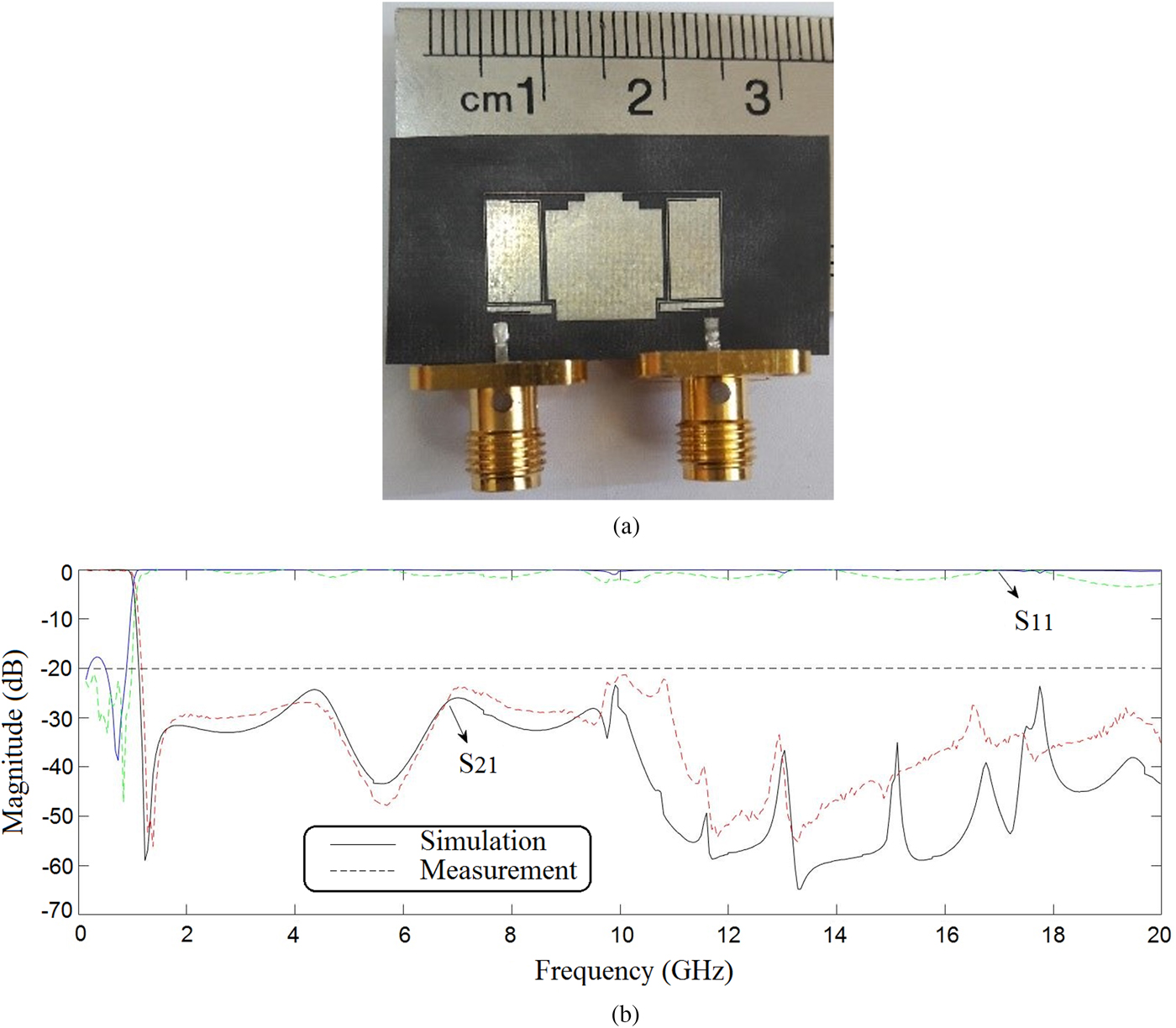
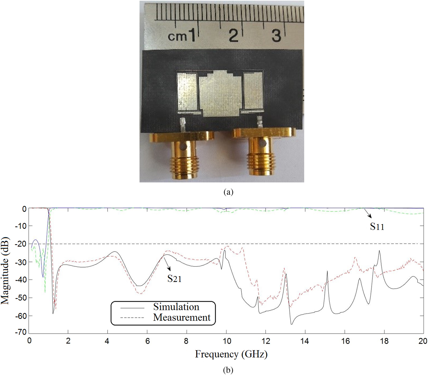
The proposed LPF is designed and simulated using ADS software (advanced design system). The proposed filter is fabricated on the RT/Duroid 5880 substrate with the thickness of 15 mil, dielectric constant ε r = 2.2, and loss tangent of 0.0009 and the measurements are performed by an HP8757A network analyzer. The photograph of the fabricated filter and its frequency responses are shown in Figs 6(a) and 6(b), respectively. As can be seen, the simulation and measurement results of the proposed LPF are in good agreement. The fabricated LPF has good characteristics such as wide stopband from 1.1 to 20 GHz, high attenuation level in the stopband and a sharp roll off. Also, the simulation and measurement insertion loss are 0.081 and 0.415 dB, respectively, which is very suited compared to the previous work. Filter's insertion loss depends on source and load impedances. The difference between simulated and measured insertion loss results from the mismatching of ports in the fabricated circuit.
(a) Filter made. (b) The results of simulation and fabrication.
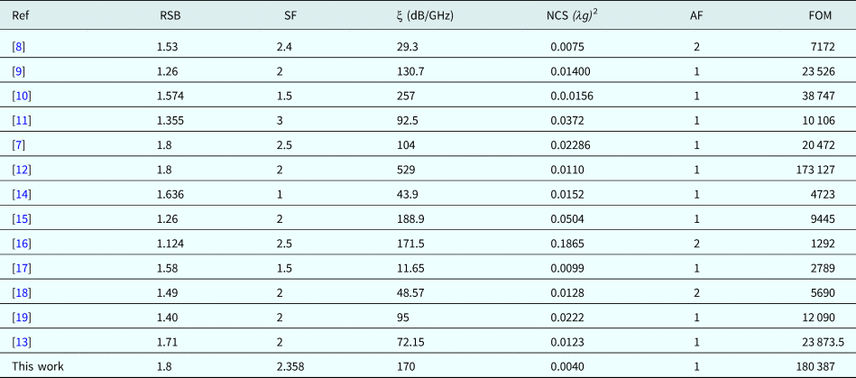
In Table 3, a comparison between the proposed LPF and the other published works is shown, where parameters RSB, SF, ξ (dB/GHz), NCS (λg)2, AF and FOM correspond to RSB, suppressing factor (SF), roll-off rate, NCS, architecture factor (AF), and FOM, respectively [Reference Hayati, Khodadoost and Abbasi13].
Comparison of the proposed filter with other published works

The RSB is:
 $${\rm RSB} = \displaystyle{{{\rm stopband\ bandwidth}} \over {{\rm stopband\;centre\;frequency}}}.$$
The SF is:
 $${\rm SF} = \displaystyle{{{\rm maximum\;suppression\;level\;in\;stopband\;} \lpar {{\rm dB}} \rpar } \over {10}}.$$
The roll-off rate (ξ) dB/GHz is:
 $$\xi = \displaystyle{{{\rm \;} \alpha _{\max} -{\rm \;} \alpha _{{\rm \; min}}} \over {\,f_s-f_c}},$$
where α min and α max denote the 3 and 20 dB attenuation points of the S21 chart, respectively. f s is the 20 dB stopband frequency, and f c is the 3 dB cut-off frequency.
The NCS λg 2 is:
 $${\rm NCS\;} = \displaystyle{{{\rm physical}\,\,{\rm size}} \over {{(\lambda g)}^2}}.$$
The AF is signed as 1 when the design is 2D and as 2 when the design is 3D.
The FOM is:
 $${\rm FOM} = \displaystyle{{\xi \times {\rm RSB} \times {\rm SF}} \over {{\rm AF} \times {\rm NCS}}}.$$
The comparison between the proposed LPF and the other works shows better performance of the proposed LPF. Also, the proposed LPF as shown in Table 3 has a high FOM of 180 387.
Conclusion
In this paper, an LPF with a sharp response and a flat passband is designed. According to the measurement results, a return loss equal to 17.65 dB, a roll-off rate of 170 dB/GHz, and a wide bandwidth have been obtained. The stopband of the proposed filter is from 1.1 upto 20 GHz. One of the most prominent criteria of the proposed filter is its NCS, which is 0.0040. This value is much smaller than the other papers and has a significant impact on the FOM of the filter. Another advantage of the proposed filter is high RSB rate of 1.8, which is acceptable compared to the previous works. The proposed LPF with such characteristics is applicable for telecommunication systems.
 Seyed Hamed Kazemi was born in Kermanshah, Iran, in 1993. He received the B.Sc. degree in Telecommunication Engineering from the Kermanshah University of Technologies, Kermanshah, Iran, in 2016 and the M.Sc. degree in Electronic Engineering in 2018 from Razi University of Kermanshah. His research interests include design and analysis of the microwave circuits, microstrip filters, and couplers.
 Mohsen Hayati received the B.E. degree in Electronics and Communication Engineering from Nagarjuna University, Andhra Pradesh, India, in 1985, and the M.E. and Ph.D. degrees in Electronics Engineering from Delhi University, Delhi, India, in 1987 and 1992, respectively. He joined the Electrical Engineering Department, Razi University, Kermanshah, Iran, as an Assistant Professor in 1993. Currently, he is a Professor with the Electrical Engineering Department, Faculty of Engineering, Razi University. He has published more than 218 papers in international, domestic journals, and conferences. His current research interests include microwave and millimeter wave devices and circuits, power amplifiers, low-noise amplifier design, application of computational intelligence, artificial neural networks, fuzzy systems, neuro-fuzzy systems, electronic circuit synthesis, modeling, and simulations.