1 Introduction
Since the seminal work of Lighthill (Reference Lighthill1952), many numerical and experimental studies have been devoted to the identification and description of the noise sources in compressible subsonic free jets with the aim of modelling the noise production mechanisms and predicting the sound propagation to the far field (see among many the papers of Lilley (Reference Lilley1991), Goldstein (Reference Goldstein1984), Viswanathan (Reference Viswanathan2006)). Recent papers (see Cavalieri et al. (Reference Cavalieri, Jordan, Agarwal and Gervais2011) and Cavalieri et al. (Reference Cavalieri, Rodríguez, Jordan, Colonius and Gervais2013)) have shown that the noise propagated to the far field is related to unsteady turbulent structures in the shear layer and to their mutual interactions along the jet flow. However, a clear picture of the nature of the flow structures generating noise is not yet available and further efforts in this field are needed. To this extent, it is known that the investigation of the pressure field in a region close to the jet flow may help to identify the noise sources and better characterize the sound production mechanisms with respect to the analysis of the far-field pressure fluctuations. For these reasons, the near field of free jets has been the subject of several experimental and numerical studies in the literature (e.g. Fuchs Reference Fuchs1972; Ukeiley & Ponton Reference Ukeiley and Ponton2004; Suzuki & Colonius Reference Suzuki and Colonius2006; Bogey, Marsden & Bailly Reference Bogey, Marsden and Bailly2012b ). Nevertheless, the physical interpretation of a pressure signal taken in the proximity of a jet is definitely tricky. As pointed out by Howes (Reference Howes1960), a microphone in the near field is subjected to the pressure fluctuations associated with the hydrodynamic structures convected inside the jet and the perturbations induced by the propagating acoustic waves. As firstly suggested by Ribner (Reference Ribner1962), a distinction between ‘sound’ and ‘pseudo-sound’ can be made in the near field of a jet. The pseudo-sound, also called hydrodynamic component, is weakly influenced by compressibility (Ffowcs Williams Reference Ffowcs Williams1969), and does not radiate. On the other hand, the sound or acoustic component is associated with sound waves propagating at the speed of sound and governed by the linear wave equation (Ristorcelli Reference Ristorcelli1997).
The necessity to separate the acoustic pressure from the hydrodynamic perturbations (which does not mean isolating the acoustic sources in the jet) was explicitly addressed by Tinney et al. (Reference Tinney, Jordan, Hall, Delville and Glauser2007) for the case of compressible jets. Such a separation could be achieved by a proper filtering procedure since, as pointed out by Arndt, Long & Glauser (Reference Arndt, Long and Glauser1997), the hydrodynamic component is dominant in the low-frequency region of the spectrum, whereas the acoustic component is predominant at high frequencies. A Fourier filtering procedure for the separation of hydrodynamic and acoustic pressures in the near field was presented by Kerhervé et al. (Reference Kerhervé, Guitton, Jordan, Delville, Fortuné, Gervais and Tinney2008) and Tinney & Jordan (Reference Tinney and Jordan2008). Pseudo-sound and sound pressures were isolated on the basis of their phase velocity in the wavenumber–frequency spectrum. In the authors’ opinion, the only drawback of such method is represented by the large number of near-field microphones required to provide a satisfactory resolution in the wavenumber domain. Further details on this technique will be given below.
It is well known that hydrodynamic pressure, being induced by the turbulent structures inside the jet, is intrinsically intermittent (see Juvé, Sunyach & Comte-Bellot Reference Juvé, Sunyach and Comte-Bellot1980; Camussi & Guj Reference Camussi and Guj1997, Reference Camussi and Guj1999; Kearney-Fischer, Sinha & Samimy Reference Kearney-Fischer, Sinha and Samimy2013). This physical evidence motivated the use of the wavelet decomposition rather than the Fourier transform for the analysis of vorticity and hydrodynamic pressure in turbulent flows. Indeed, as pointed out by Ruppert-Felsot, Farge & Petitjeans (Reference Ruppert-Felsot, Farge and Petitjeans2009), the Fourier modes are not well suited to represent and describe intermittent events since they are localized in the spectral space but not in the physical one. Therefore, the use of a wavelet basis is more advisable due to its localization in both the physical and the transformed spaces. With the purpose of analysing the near-field pressure, such an idea was exploited by Grizzi & Camussi (Reference Grizzi and Camussi2012), who developed a wavelet-based procedure to separate hydrodynamic and acoustic pressures. They assumed that the hydrodynamic contribution related to localized eddy structures compresses well onto a wavelet basis so that it can be described by a few but with large amplitude wavelet coefficients. Thus, the pseudo-sound can be extracted by selecting the wavelet coefficients exceeding a proper threshold. The acoustic counterpart associated with more homogeneous and low-energy fluctuations is represented by those coefficients having an amplitude lower than the threshold. The advantage of this wavelet-based method with respect to previous approaches was mainly in the simplicity of the required set-up. Indeed, only two microphone signals in the near field, acquired (or computed) in two positions sufficiently close to each other, are needed to compute the cross-correlation between the presumed hydrodynamic and acoustic components. The computation of the cross-correlation was necessary to determine through an iterative process the amplitude of the threshold level mentioned above (see Grizzi & Camussi (Reference Grizzi and Camussi2012) for the details).
The above discussion motivated the present work in which novel wavelet-based methods are presented with the aim of improving the efficiency of the method proposed by Grizzi & Camussi (Reference Grizzi and Camussi2012) and further simplifying the set-up required for the practical application of the procedure (e.g. by using only one microphone). Three new wavelet-based methods are presented and the main concepts underlying these approaches are the following:
-
(i) the separation between hydrodynamic and acoustic pressures is accomplished through the estimation of the cross-correlation between near- and far-field pressures measured simultaneously using two microphones. It is expected that the near-field acoustic pressure correlates well with the far-field noise;
-
(ii) the near-field acoustic pressure is extracted through an iterative process based on the degree of similarity between the probability density functions of the near- and far-field pressure fluctuations, the latter being assumed as Gaussian. The application of such a procedure requires only one microphone in the near field;
-
(iii) the hydrodynamic pressure is filtered out through the application of the technique proposed by Ruppert-Felsot et al. (Reference Ruppert-Felsot, Farge and Petitjeans2009) for the extraction of coherent structures in a vorticity field. As for the previous case, also this method requires the use of only one microphone in the near field.
More details on the procedures will be given below. Here, it is only pointed out that one of the major properties of these new data processing procedures is that their application requires a very simple experimental set-up consisting of only one microphone in the near field or, for the method (i), of two microphones, one in the near field and one in the far field.
The methods are applied to simultaneous near- and far-field pressure data measured around a subsonic jet installed within the anechoic chamber available at the Centre Acoustique of Laboratoire de Mécanique des Fluides et d’Acoustique at the École Centrale de Lyon. A statistical and spectral characterization of the separated hydrodynamic and acoustic components is provided highlighting the effect of the axial location of the near-field microphone in the streamwise direction and the effect of the jet Mach number. In order to validate the techniques, the Fourier filtering technique derived by Tinney & Jordan (Reference Tinney and Jordan2008) as well as the wavelet-based separation procedure proposed by Grizzi & Camussi (Reference Grizzi and Camussi2012) are also applied to the present database.
The paper is organized as follows: § 2 is devoted to the description of the novel wavelet-based separation techniques. Section 3 provides a description of the experimental set-up and a characterization of the jet flow. Main results concerning the separation and the statistical and spectral characterization of the hydrodynamic and acoustic pressures are shown in § 4, and conclusions are presented in § 5.
2 Wavelet-based techniques for the hydrodynamic/acoustic near-field pressure separation
The separation between hydrodynamic and acoustic components of the near-field pressure is based on the application of the wavelet transform to pressure signals. The reader may refer to Mallat (Reference Mallat1989), Daubechies (Reference Daubechies1992), Torrence & Compo (Reference Torrence and Compo1998) and Farge (Reference Farge1992) for comprehensive reviews on mathematical aspects of wavelet transforms and their applications.
The continuous wavelet transform (CWT) of a pressure time signal
 $p(t)$
consists of a projection over a basis of compact support functions obtained by dilations and translations of the so-called mother wavelet
 $\unicode[STIX]{x1D6F9}(t)$
. The mother wavelet is localized both in the physical and transformed spaces, the resulting wavelet coefficients being function of the time
 $t$
and of the scale
 $s$
, which is inversely proportional to the frequency (Meyers, Kelly & O’Brien Reference Meyers, Kelly and O’Brien1993). According to Grizzi & Camussi (Reference Grizzi and Camussi2012), the CWT of a time signal can be defined as follows:
 $$\begin{eqnarray}\displaystyle w_{p}(s,t)=C_{\unicode[STIX]{x1D713}}^{-1/2}\int _{-\infty }^{+\infty }p(\unicode[STIX]{x1D70F})\unicode[STIX]{x1D6F9}^{\ast }\left(\frac{t-\unicode[STIX]{x1D70F}}{s}\right)\,\text{d}\unicode[STIX]{x1D70F}, & & \displaystyle\end{eqnarray}$$
where
 $C_{\unicode[STIX]{x1D713}}^{-1/2}$
is a constant to take into account the mean value of
 $\unicode[STIX]{x1D6F9}(t)$
and
 $\unicode[STIX]{x1D6F9}^{\ast }((t-\unicode[STIX]{x1D70F})/s)$
is the complex conjugate of the dilated and translated
 $\unicode[STIX]{x1D6F9}(t)$
.
Instead of a continuous wavelet transform, a discrete wavelet transform can be adopted to decompose the signal
 $p(t)$
. According to Meneveau (Reference Meneveau1991), if the scales
 $s_{j}$
are arranged on a dyadic distribution, i.e.
 $s_{j}=2^{j}$
, and the considered translations are a multiple of the scale
 $s_{j}$
, the orthonormal basis
 $\unicode[STIX]{x1D713}(t)$
obtained by dilations and translations of the mother wavelet
 $\unicode[STIX]{x1D6F9}(t)$
can be represented by the following formula:
 $$\begin{eqnarray}\displaystyle \unicode[STIX]{x1D713}_{[k]}^{(j)}(t)=2^{-j/2}\unicode[STIX]{x1D6F9}\left(\frac{t-2^{j}k}{2^{j}}\right). & & \displaystyle\end{eqnarray}$$
The discrete wavelet coefficients are obtained as follows:
 $$\begin{eqnarray}\displaystyle w_{p}^{(s)}(n)=\mathop{\sum }_{k=-\infty }^{+\infty }\unicode[STIX]{x1D6F9}^{(s)}(n-2^{s}k)p(k). & & \displaystyle\end{eqnarray}$$
Where
 $s$
represents the discretized scale, whereas the wavelet function
 $\unicode[STIX]{x1D6F9}^{(s)}(n-2^{s}k)$
is the discretized version of
 $\unicode[STIX]{x1D6F9}^{(s)}(t)=2^{-s/2}\unicode[STIX]{x1D6F9}(t/2^{s})$
(Camussi & Guj Reference Camussi and Guj1997).
In the present approach, the wavelet transform is performed using an orthogonal wavelet basis to ensure the reversibility condition and the wavelet kernel used is the Daubechies–12 type. In order to ensure the generality of the present approaches, it has been checked that the results presented in the following do not depend on the choice of the wavelet type. In all cases, the analysis is carried out using the Matlab® wavelet toolbox.
According to the approach proposed by Grizzi & Camussi (Reference Grizzi and Camussi2012), it is assumed that the hydrodynamic component of the near-field pressure, being related to localized vortices, compresses well onto the wavelet basis. Therefore, the component of the signal associated with the hydrodynamic pressure can be extracted by selecting the wavelet coefficients exceeding, in absolute value, a proper threshold, the remaining part of the signal being assumed as acoustic pressure.
It is clear that the selection of the threshold represents a crucial step in the separation procedure and its selection has to be related to physical properties of the hydrodynamic or acoustic pressure components. The distinction among the three procedures introduced therein is indeed mainly based on the way the threshold is selected.
An initial guess for the threshold value
 $T_{0}$
is adopted for all the techniques and it is based on statistical reasoning introduced in the de-noising procedure developed by Donoho & Johnstone (Reference Donoho and Johnstone1994):
 $$\begin{eqnarray}\displaystyle T_{0}=\sqrt{2\langle p^{\prime 2}\rangle \log _{2}N_{s}}, & & \displaystyle\end{eqnarray}$$
where
 $\langle p^{\prime 2}\rangle$
is the variance of the pressure signal and
 $N_{s}$
is the number of samples. The threshold is discretely changed until a proper convergence criterion capturing the hydrodynamic or acoustic nature of the separated signals is satisfied. The iterative process differs for each technique being different the physical aspect to which the separation procedure is related. It will be shown that whatever is the initial hypothesis and the objective function to be satisfied, all the separation techniques lead to very similar results.
Hereinafter, in order to simplify the description, the original near-field pressure signal will be denoted as
 $p_{NF}$
, the near-field hydrodynamic and acoustic pressure signals as
 $p_{H}$
and
 $p_{A}$
respectively and the far-field pressure signal as
 $p_{FF}$
.
2.1 Wavelet technique ‘WT1’
The separation technique denoted as WT1 requires one microphone in the near field and one microphone in the far field. The iterative process for the selection of the threshold is based on the computation of the cross-correlation between the guessed acoustic component of the near-field pressure and the measured far-field pressure. The cross-correlation function, establishing a causality relation between the convoluted time series (Bogey & Bailly Reference Bogey and Bailly2007), is considered as an indicator of the degree of similarity between the two pressure signals. Indeed, the hypothesis at the basis of the procedure is that the amplitude of the hydrodynamic fluctuations decreases very rapidly by increasing the radial distance from the jet (Suzuki & Colonius Reference Suzuki and Colonius2006) so that the near-field acoustic component is the only one to reach the far field and thus is the only one to provide a high-value correlation with the far-field noise.
Starting from the initial guess
 $T_{0}$
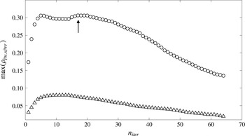
, the threshold level is varied according to a gradient-based method optimization until the cross-correlation peak between the acoustic pressure in the near field and the noise emitted in the far field exhibits a maximum. As an example, figure 1 shows the variation of the peak of the cross-correlation coefficient between either the separated hydrodynamic or acoustic component and the far-field pressure, as a function of the number of iterations. It is observed that the correlation between the acoustic and the far-field pressure is always much larger than the one between the hydrodynamic and the far-field pressure. Starting from the initial guess defined above, as the threshold value varies the acoustic cross-correlation peak increases rapidly until it reaches a quasi-constant trend, after which the maximum of the cross-correlation peak is reached. For such a threshold level the convergence criterion is satisfied and the pseudo-sound and sound pressures are separated successfully.
Separation technique WT1: cross-correlation coefficient peak along the number of iterations of the acoustic and hydrodynamic components with the measured far-field pressure. ▵ hydrodynamic pressure, ○ acoustic pressure. Jet Mach number
 $M_{j}=0.6$
, near-field microphone axial location
 $x/D=8.7$
, far-field microphone polar position
 $\unicode[STIX]{x1D713}=140^{\circ }$
. The separation point for which the convergence criterion is satisfied is highlighted with an arrow.

2.2 Wavelet technique ‘WT2’
In the method denoted as WT2 the iterative process for the threshold level selection is based on the computation of the probability density function (PDF) of the guessed near-field acoustic pressure and its comparison with a Gaussian distribution that is assumed to be the PDF of the actual acoustic pressure. As it will be shown below, the analysis of the far-field pressure confirms this assumption.
The separation procedure adopted is summarized in the following steps. Starting from the initial guess
 $T_{0}$
, the threshold value is iteratively decreased by 5 %. At each iteration the normalized probability density function of the guessed near-field acoustic pressure, denoted as
 $\text{PDF}_{A}$
, is computed and compared with a reference standard Gaussian distribution
 $\text{PDF}_{g}$
. The estimation of the similarity between the two PDFs is accomplished through a ‘
 $\unicode[STIX]{x1D712}$
squared test’ (Chernoff & Lehmann Reference Chernoff and Lehmann1954). The iterative process ends when the departure of
 $\text{PDF}_{A}$
from the normal distribution is less than a tolerance
 $\unicode[STIX]{x1D716}$
, formalized as follows:
 $$\begin{eqnarray}\displaystyle \unicode[STIX]{x1D712}^{2}=\mathop{\sum }_{k=1}^{N_{bin}}\frac{(\text{PDF}_{A_{k}}-\text{PDF}_{g_{k}})^{2}}{\text{PDF}_{g_{k}}}<\unicode[STIX]{x1D716}, & & \displaystyle\end{eqnarray}$$
where
 $\unicode[STIX]{x1D716}$
has been set equal to
 $10^{-4}$
, whereas
 $N_{bin}$
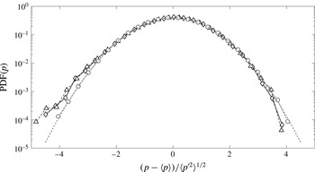
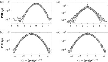
is the number of bins used to compute the PDF for a discrete series of values. Figure 2 shows examples of PDFs of the original and the separated signals compared with the standard Gaussian distribution. The agreement between the acoustic and Gaussian PDFs is well verified, thus implying that the sound component can be handled as a stochastic and statistically steady phenomenon. On the contrary, the original and the hydrodynamic PDFs exhibit a significant discrepancy in the tails due to intermittent pressure events associated with the turbulence development. Further discussions and physical interpretations of this behaviour will be given in § 4.
Separation technique WT2: probability density functions of original, hydrodynamic and acoustic pressures and comparison with the normalized standard Gaussian distribution. ♢ original pressure, ▵ hydrodynamic pressure, ○ acoustic pressure, dashed line corresponds to the standard Gaussian distribution. Jet Mach number
 $M_{j}=0.6$
, microphone axial position
 $x/D=5.6$
.

2.3 Wavelet technique ‘WT3’
The third separation procedure, denoted as WT3, is an application to the pressure field of the decomposition technique developed by Ruppert-Felsot et al. (Reference Ruppert-Felsot, Farge and Petitjeans2009) to extract coherent structures from a vorticity field. The assumption at the basis of the present approach is that the hydrodynamic pressure is related to temporally and spatially localized coherent turbulent structures convected by the jet flow. On the basis of the relation between hydrodynamic pressure and vorticity (see e.g. Landau & Lifshitz (Reference Landau and Lifshitz1985) and more recently Hanjalić & Mullyadzhanov (Reference Hanjalić and Mullyadzhanov2015)), it is straightforward to assume that the method adopted in Ruppert-Felsot et al. (Reference Ruppert-Felsot, Farge and Petitjeans2009) to extract the coherent structures of the vorticity field can be efficiently used to isolate the hydrodynamic pressure (associated with the coherent vorticity) from the acoustic counterpart.
The separation algorithm is based on the application of a recursive de-noising procedure in which the acoustic pressure field is iteratively evaluated until a convergence criterion is satisfied. Starting from the initial guess
 $T_{0}$
defined above, the threshold value is updated at each
 $k$
th iteration according to the following formula:
 $$\begin{eqnarray}\displaystyle T_{k}=\sqrt{2\langle p_{A}^{\prime 2}\rangle |_{k}\log _{2}N_{s}}, & & \displaystyle\end{eqnarray}$$
where
 $\langle p_{A}^{\prime 2}\rangle |_{k}$
is the variance of the acoustic pressure signal at each iteration. The pseudo-sound and sound components are iteratively separated being their wavelet coefficients respectively larger or lower than the updated threshold level. A convergence analysis of the threshold value as a function of the number of samples has been preliminarily carried out in order to verify that the resulting decomposition was independent of the number of samples for
 $N_{s}\geqslant N_{s}^{\ast }$
. The value of
 $N_{s}^{\ast }$
was found to be equal to
 $2^{18}$
for all the analysed signals. The iterative process stops when the number of wavelet coefficients of the acoustic pressure becomes constant (see also Azzalini, Farge & Schneider (Reference Azzalini, Farge and Schneider2005)).
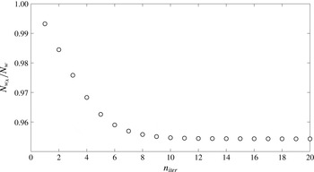
Figure 3 clarifies the procedure. It shows for a reference case the number of wavelet coefficients of the acoustic pressure (
 $N_{w_{A}}$
) normalized with respect to the total number of wavelet coefficients of the original pressure signal (
 $N_{w}$
) as a function of the iterations. It is observed that, after a certain number of iterations,
 $N_{w_{A}}$
remains constant thus indicating that the iterative process has converged. This trend has been observed in all cases examined therein and for all the analysed signals the convergence has been achieved after a number of iterations of the order of 20.
Separation technique WT3: trend along the iterations of the number of wavelet coefficients of the acoustic pressure normalized by the total number of the wavelet coefficients of the original signal. Jet Mach number
 $M_{j}=0.6$
, microphone axial position
 $x/D=7.4$
.

3 Experimental set-up and jet assessment
3.1 Facility description and instrumentation
The experimental test campaign has been carried out in the anechoic wind tunnel available at the Centre Acoustique of Laboratoire de Mécanique des Fluides et d’Acoustique at the École Centrale de Lyon. The fully anechoic chamber size is
 $10\times 9\times 8~\text{m}^{3}$
. The feed line consists of a compressed dry air duct supplied by a compressor delivering a continuous mass flow rate of up to
 $1~\text{kg}~\text{s}^{-1}$
. An electrically driven valve downstream of the compressor permits the regulation of the jet velocity by controlling the incoming mass flow. The flow conditions are continuously monitored by a thermocouple and a pressure tap located 15 jet diameters upstream the nozzle exit, which permit to measure respectively the total temperature and the static pressure of the inflow. The jet exit conditions are obtained by use of isentropic flow relations between the pressure and temperature measurements and the nozzle exit conditions. Analytical predictions were verified by ad hoc Pitot measurements.
Experiments were performed on a single-stream round jet for two Mach numbers:
 $M_{j}=0.6$
and
 $M_{j}=0.9$
, to which correspond Reynolds numbers respectively equal to
 $Re_{D}\approx 7.5\times 10^{5}$
and
 $Re_{D}\approx 1.2\times 10^{6}$
, which classify the jet as a high Reynolds number jet (Bogey, Marsden & Bailly Reference Bogey, Marsden and Bailly2012a
; Viswanathan Reference Viswanathan2004).
 $Re_{D}$
denotes the Reynolds number based on the nozzle diameter
 $D=50~\text{mm}$
and on the flow velocity at the nozzle exit
 $U_{j}=M_{j}c_{j}$
,
 $c_{j}$
being the speed of sound.
Velocity measurements were carried out in order to provide a preliminary characterization of the aerodynamic field in the jet plume. The measurements were performed by a single hot-wire probe DANTEC 55P11 of
 $1~\text{mm}$
length and
 $5~\unicode[STIX]{x03BC}\text{m}$
diameter. The hot-wire was mounted on a traversing system with the probe in the normal direction with respect to the jet flow in order to reduce the flow disturbances. The hot-wire was connected to a constant temperature anemometer system DANTEC Streamline Pro. Velocity signals were acquired by a National Instruments PXI-4472 acquisition system with a sampling frequency set to
 $25.6~\text{kHz}$
for an acquisition time of
 $10~\text{s}$
.
Simultaneous near- and far-field pressure measurements have been carried out in free-jet conditions. Pressure fluctuations were measured by PCB 377B01 microphones, whose frequency response is flat in the
 $4~\text{Hz}$
–
 $80~\text{kHz}$
range and whose full-scale value is
 $165~\text{dB}$
. Pressure signals were acquired by National Instruments PXI-4472 system with a sampling frequency equal to
 $51.2~\text{kHz}$
for an acquisition time of
 $10~\text{s}$
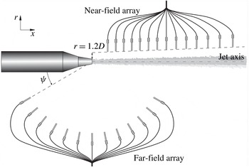
. A near-field 14 microphone linear array was placed at a radial distance of
 $r/D=1.2$
from the jet in the so-called ‘linear hydrodynamic regime’, in which a superimposition of the hydrodynamic and acoustic pressures is found (Suzuki & Colonius Reference Suzuki and Colonius2006). The array was aligned to the jet spreading angle, which was found to be close to
 $11^{\circ }$
from the overall aerodynamic characterization by hot-wire measurements. The microphones were not equally spaced along the streamwise direction spanning an axial distance from the nozzle exhaust from
 $x/D=2$
to
 $x/D=8.7$
. The far-field microphones were located on a circular arc at a radial distance from the nozzle exit
 $r/D=40$
on a polar angle range spanning from
 $30^{\circ }$
to
 $150^{\circ }$
, the polar angle
 $\unicode[STIX]{x1D713}$
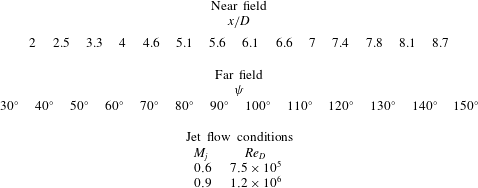
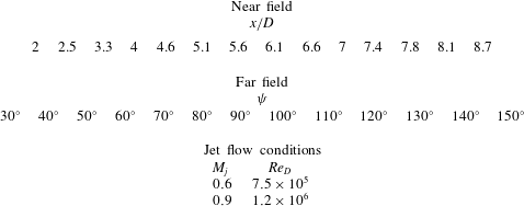
being defined positive in the upstream direction. A sketch of the experimental set-up is shown in figure 4. A summary of the jet flow conditions analysed and of the microphones’ disposition is reported in table 1.
Resume of the jet flow conditions analysed and of the location of the near- and far-field microphones.
Sketch of the experimental set-up and scheme of the microphones’ disposition.

3.2 Jet characterization
The aerodynamic characterization of the jet is provided in terms of mean velocity and turbulence intensity profiles along the radial distance
 $r$
for different axial positions
 $x$
of the hot-wire. The mean and fluctuating velocities at each position were normalized by the jet velocity at the nozzle exit
 $U_{j}$
, whereas a non-dimensional radial coordinate
 $\unicode[STIX]{x1D702}$
was computed according to the following formula:
 $$\begin{eqnarray}\displaystyle \unicode[STIX]{x1D702}=\frac{r-R_{1/2}}{\unicode[STIX]{x1D6FF}_{\unicode[STIX]{x1D703}}}. & & \displaystyle\end{eqnarray}$$
Where
 $r$
is the radial distance from the jet axis,
 $R_{1/2}$
is the radial position for which the mean axial velocity is 50 % of the jet velocity and
 $\unicode[STIX]{x1D6FF}_{\unicode[STIX]{x1D703}}$
is the momentum thickness of the shear layer defined as follows:
 $$\begin{eqnarray}\displaystyle \unicode[STIX]{x1D6FF}_{\unicode[STIX]{x1D703}}=\int _{-\infty }^{+\infty }\frac{\langle U\rangle }{\langle U(r=0)\rangle }\left(1-\frac{\langle U\rangle }{\langle U(r=0)\rangle }\right)\,\text{d}r. & & \displaystyle\end{eqnarray}$$
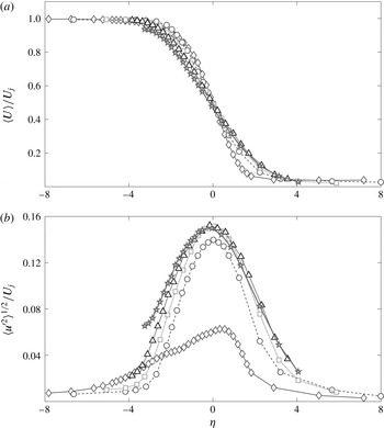
Figure 5 shows the dimensionless velocity and turbulence level profiles for the axial distances
 $x/D=0$
,
 $1$
,
 $3$
,
 $5$
,
 $7$
. For the sake of conciseness, we just considered the case
 $M_{j}=0.6$
. The shape and the evolution along the axial distance of the mean and fluctuating velocity profiles are in agreement with previous results found in the literature (Moore Reference Moore1977; Jung, Gamard & George Reference Jung, Gamard and George2004). The mean velocity profiles exhibit the typical top-hat shape with a velocity value approximately constant along the jet centreline up to
 $5$
diameters downstream of the nozzle exhaust. The relative turbulence level based on the jet velocity is approximately
 $1$
% on the jet axis close to the nozzle exhaust, it increases moving downstream in the jet and inside the shear layer reaching a maximum value of
 ${\approx}16$
% for
 $\unicode[STIX]{x1D702}=0$
.
Dimensionless mean and fluctuating velocity profiles along the non-dimensional radial coordinate
 $\unicode[STIX]{x1D702}$
at different axial positions
 $x$
for jet Mach number
 $M_{j}=0.6$
: (a) mean velocity, (b) relative turbulence level. ♢
 $x/D=0$
, ○
 $x/D=1$
, ▫
 $x/D=3$
, ▵
 $x/D=5$
,
 $\star$
 $x/D=7$
.

The aeroacoustic qualification of the jet is carried out by analysing both the near- and the far-field pressure data. The statistical description of the far-field pressure also provides a demonstration of the Gaussian nature of the pressure fluctuations far away from the jet, a result which is fundamental for the application of the method denoted in the previous section as WT2.
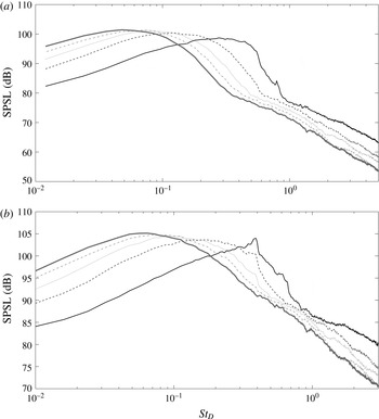
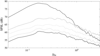
Figure 6 shows the streamwise evolution of the near-field sound pressure spectrum levels (SPSLs) for axial positions
 $x/D=2.5$
,
 $4.6$
,
 $6.1$
,
 $7.4$
and
 $8.7$
and for the two Mach numbers considered herein. According to Pierce (Reference Pierce1981) and Di Marco, Mancinelli & Camussi (Reference Di Marco, Mancinelli and Camussi2015), the SPSL is computed as follows:
 $$\begin{eqnarray}\displaystyle \text{SPSL}=10\log _{10}\frac{\text{PSD}\unicode[STIX]{x0394}f_{ref}}{p_{ref}^{2}}, & & \displaystyle\end{eqnarray}$$
where PSD is the power spectral density.
 $\unicode[STIX]{x0394}f_{ref}=1~\text{Hz}$
and
 $p_{ref}=20~\unicode[STIX]{x03BC}\text{Pa}$
are the reference frequency and the reference pressure respectively. The pressure spectra are represented as a function of the Strouhal number
 $St_{D}=fD/U_{j}$
. It is observed that, as the axial distance from the nozzle exit increases, the energy hump in the spectra moves from high to low-frequency range, such a behaviour being related to the development of larger turbulent structures. For small axial distances an energy peak at a Strouhal number
 ${\approx}0.39$
associated with the Kelvin–Helmholtz instability mode (Danaila, Dušek & Anselmet Reference Danaila, Dušek and Anselmet1997) clearly emerges for
 $M_{j}=0.9$
, whereas for the case
 $M_{j}=0.6$
higher-order harmonics are detected. Moving downstream, the turbulence intensity increases and the spectral shape changes accordingly showing a broadband energy distribution.
Axial evolution of the pressure spectra: (a) jet Mach number
 $M_{j}=0.6$
, (b) jet Mach number
 $M_{j}=0.9$
. Solid lines
 $x/D=2.5$
, dashed lines
 $x/D=4.6$
, dotted lines
 $x/D=6.1$
, dash-dotted lines
 $x/D=7.4$
, bold lines
 $x/D=8.7$
.

As pointed out by Arndt et al. (Reference Arndt, Long and Glauser1997), the energy content associated with the pressure fluctuations shows far-field behaviour when the product between the axial wavenumber
 $k_{x}$
and the radial distance
 $r$
is sufficiently large (
 $k_{x}r\gg 1$
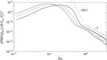
). According to this condition, the near-field pressure spectra are characterized by a dominant hydrodynamic component at low frequencies, whereas the acoustic component prevails at high frequencies. Such aspect is confirmed by the different energy decay laws found in the pressure spectra. Figure 7 shows the dimensionless spectra at
 $x/D=3.3$
,
 $4.6$
,
 $5.6$
,
 $6.1$
and for
 $M_{j}=0.6$
. The PSDs have been normalized by the dynamic pressure computed using as reference density the ambient air density
 $\unicode[STIX]{x1D70C}_{\infty }=1.225~\text{kg}~\text{m}^{-3}$
and as reference velocity the jet velocity
 $U_{j}$
. It is observed that at low frequencies the spectra show an energy decay
 $\propto St_{D}^{-20/3}$
typical of the hydrodynamic fluctuations, while at high frequencies a slope of
 $-2$
related to pressure perturbations induced by sound waves is observed (Arndt et al.
Reference Arndt, Long and Glauser1997; Tinney et al.
Reference Tinney, Jordan, Hall, Delville and Glauser2007).
Dimensionless pressure spectra for jet Mach number
 $M_{j}=0.6$
at different axial distances: solid line corresponds to
 $x/D=3.3$
, dashed line to
 $x/D=4.6$
, dotted line to
 $x/D=5.6$
, dash-dotted line to
 $x/D=6.1$
.

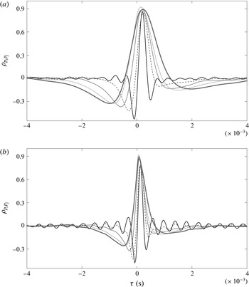
The interpretation of the spectra is confirmed by the analysis of the axial evolution of the cross-correlation coefficient (Ross Reference Ross2014), as shown in figure 8. The cross-correlation has been computed between two consecutive microphones of the near-field array. At small axial distances a pseudo-periodic behaviour is observed, such a trend being again the signature of the Kelvin–Helmholtz instability mode. Moving downstream from the jet exit, the turbulence development produces the typical negative–positive bump shape (Grizzi & Camussi Reference Grizzi and Camussi2012), the larger correlation time scale being related to the development of large-scale turbulent structures.
Axial evolution of the cross-correlation coefficient between two consecutive microphone signals in the near field: (a) jet Mach number
 $M_{j}=0.6$
, (b) jet Mach number
 $M_{j}=0.9$
. Solid lines
 $x/D=2$
–
 $2.5D$
, dashed lines
 $x/D=4$
–
 $4.6$
, dotted lines
 $x/D=5.6$
–
 $6.1$
, dash-dotted lines
 $x/D=7$
–
 $7.4$
, bold lines
 $x/D=8.1$
–
 $8.7$
.

Figure 9 shows the polar evolution of the far-field pressure spectra for polar angles
 $\unicode[STIX]{x1D713}=150^{\circ }$
,
 $130^{\circ }$
,
 $110^{\circ }$
,
 $90^{\circ }$
,
 $70^{\circ }$
and for
 $M_{j}=0.9$
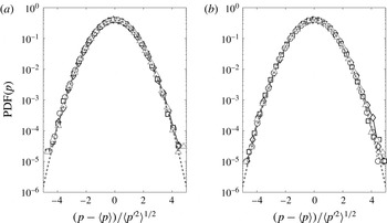
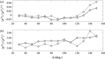
. As expected, the noise level as well as the spectral shape changes significantly moving from the forward to the aft arc. For large polar angles the spectra show a sharper noise peak, whereas at smaller polar angles the peak broadens and rolls off gradually. Such a trend is in agreement with the well-known prediction provided by Tam, Golebiowski & Seiner (Reference Tam, Golebiowski and Seiner1996) and Tam et al. (Reference Tam, Viswanathan, Ahuja and Panda2008) and related to the noise components associated with the large- and small-scale turbulent structures. Figure 10 shows the polar evolution of the PDFs of the far-field pressure signals for both jet Mach numbers. Experimental data were compared with the reference standard Gaussian distribution showing a good agreement. Furthermore the polar evolution of the third and fourth-order statistical moments of the far-field pressure signals is shown in figure 11. It is observed that the skewness and flatness factors exhibit values respectively equal to 0 and 3, as for the reference Gaussian distribution, for all the polar angles considered. This feature further confirms that the statistics of the far-field pressure fluctuations can be assumed as Gaussian.
Polar trend of the far-field pressure spectra for jet condition
 $M_{j}=0.9$
. Solid line
 $\unicode[STIX]{x1D713}=150^{\circ }$
, dashed line
 $\unicode[STIX]{x1D713}=130^{\circ }$
, dotted line
 $\unicode[STIX]{x1D713}=110^{\circ }$
, dash-dotted line
 $\unicode[STIX]{x1D713}=90^{\circ }$
, bold line
 $\unicode[STIX]{x1D713}=70^{\circ }$
.

Polar evolution of the PDFs of the far-field pressure for both jet conditions: (a)
 $M_{j}=0.6$
, (b)
 $M_{j}=0.9$
. ♢
 $\unicode[STIX]{x1D713}=140^{\circ }$
, ○
 $\unicode[STIX]{x1D713}=120^{\circ }$
, ▫
 $\unicode[STIX]{x1D713}=90^{\circ }$
, ▵
 $\unicode[STIX]{x1D713}=70^{\circ }$
, dashed line refers to the standard Gaussian distribution.

Polar evolution of the skewness and flatness factors of the far-field pressure for both jet conditions: ♢
 $M_{j}=0.6$
, ○
 $M_{j}=0.9$
. (a) Skewness factor, (b) kurtosis.

4 Results
In the present section the spectral and statistical analyses of the hydrodynamic and acoustic near-field pressures separated using the techniques described in § 2 are presented. The application of the methods to the experimental data provides a characterization of the pseudo-sound and sound components for different Mach numbers and shed light on the mechanisms underlying the generation of noise and its propagation in the far field. First of all an assessment of the achieved results was provided in order to validate the proposed techniques.
4.1 Filtering of the wavenumber–frequency spectrum
The authors briefly worked out the procedure presented in Kerhervé et al. (Reference Kerhervé, Guitton, Jordan, Delville, Fortuné, Gervais and Tinney2008) and Tinney & Jordan (Reference Tinney and Jordan2008) that provides interesting results shedding light on the physical nature of the hydrodynamic and acoustic pressure fluctuations. The method is based on the computation of the wavenumber–frequency spectrum obtained by the Fourier transform of the space–time pressure field
 $p(x,t)$
. As mentioned above, this approach requires measurements with a considerable number of microphones in the near field in order to provide an acceptable resolution of the spectrum in the wavenumber domain. In the authors’ opinion this constraint represents the main limitation of the method.
Formally, the two-dimensional Fourier transform of a pressure signal can be written as:
 $$\begin{eqnarray}\displaystyle \hat{p}(k_{x},\unicode[STIX]{x1D714})=\int _{-\infty }^{+\infty }p(x,t)W(x)W(t)\text{e}^{-\text{i}(k_{x}x+\unicode[STIX]{x1D714}t)}\,\text{d}x\,\text{d}t, & & \displaystyle\end{eqnarray}$$
where
 $\unicode[STIX]{x1D714}$
is the angular frequency and
 $W(x)$
and
 $W(t)$
are Hamming windowing functions respectively in the space and time domain. The wavenumber–frequency spectrum is computed as follows:
 $$\begin{eqnarray}\displaystyle P(k_{x},\unicode[STIX]{x1D714})=\hat{p}(k_{x},\unicode[STIX]{x1D714})\hat{p}^{\ast }(k_{x},\unicode[STIX]{x1D714}). & & \displaystyle\end{eqnarray}$$
Figure 12 shows the normalized
 $k-\unicode[STIX]{x1D714}$
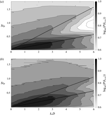
spectral map in logarithmic scale for both jet flow conditions; the map is represented against the Strouhal number and a dimensionless wavenumber based on the nozzle diameter. Two spectral lobes can be clearly observed in the Fourier domain, whose energy level and shape change depending on the jet Mach number. The two lobes are the signatures of two pressure components: the hydrodynamic pressure associated with a phase velocity comparable with the convection velocity
 $U_{c}\approx 0.6\,U_{j}$
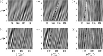
(Picard & Delville Reference Picard and Delville2000) and the acoustic pressure related to a phase velocity of the order of the speed of sound. Pseudo-sound and sound components are extracted by filtering the two-dimensional spectrum according to their phase velocities. Pressure perturbations propagating at a velocity greater than or equal to the speed of sound are related to acoustic pressure, whereas pressure fluctuations convected at a velocity lower than the speed of sound are associated with hydrodynamic pressure. Figure 13 shows the space–time map of the original pressure field and the separated hydrodynamic and acoustic pressure fields for both jet Mach numbers. The characteristic propagation velocities of each separated pressure component are superimposed to the maps. It can be observed that the hydrodynamic field shows a more coherent signature with pressure perturbations moving with a phase velocity equal to the convection velocity. On the other hand the acoustic field is characterized by a less organized structure with wave fronts propagating at a velocity close to the speed of sound.
Normalized wavenumber–frequency spectrum of the near pressure field for both jet flow conditions. (a) Jet Mach number
 $M_{j}=0.6$
, (b) jet Mach number
 $M_{j}=0.9$
. Dashed lines refer to the speed of sound, dash-dotted lines refer to the convection velocity.

 $k-\unicode[STIX]{x1D714}$
technique: space–time map of original, hydrodynamic and acoustic near pressure fields separated by the Fourier filtering technique for both jet velocities. (a) Original pressure,
 $M_{j}=0.6$
, (b) hydrodynamic pressure,
 $M_{j}=0.6$
, (c) acoustic pressure,
 $M_{j}=0.6$
, (d) original pressure,
 $M_{j}=0.9$
, (e) hydrodynamic pressure,
 $M_{j}=0.9$
, (f) acoustic pressure,
 $M_{j}=0.9$
.

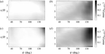
The hydrodynamic and acoustic components are correlated with the pressure measured in the far field. Figure 14 shows a map of the peaks of these cross-correlations computed for all the axial and polar positions. It is observed that the correlation between
 $p_{A}$
and
 $p_{FF}$
is larger than that between
 $p_{H}$
and
 $p_{FF}$
for all the microphone positions considered. The value of the correlation peak between
 $p_{A}$
and
 $p_{FF}$
increases as the maximum noise emissivity region in the far field is approached (
 $\unicode[STIX]{x1D713}=130^{\circ }-150^{\circ }$
). Nevertheless, in this region an unexpected high correlation level between the hydrodynamic and the far-field pressures is observed especially for
 $M_{j}=0.9$
. Such an issue can be ascribed to a lack of resolution (Kerhervé et al.
Reference Kerhervé, Guitton, Jordan, Delville, Fortuné, Gervais and Tinney2008) which affects the separation of the hydrodynamic and acoustic components mainly for low wavenumbers.
 $k-\unicode[STIX]{x1D714}$
technique: cross-correlation coefficient peak map of hydrodynamic and acoustic components with measured far-field pressure at all the axial and polar positions for both jet Mach numbers. (a) Hydrodynamic component,
 $M_{j}=0.6$
; (b) acoustic component,
 $M_{j}=0.6$
; (c) hydrodynamic component,
 $M_{j}=0.9$
; (d) acoustic component,
 $M_{j}=0.9$
.

4.2 Comparison between reference and novel techniques
In order to better appreciate the effectiveness and efficiency of the different methods and in order to enhance any differences, the results obtained by the application of the three wavelet-based techniques introduced therein are compared with each other. The validation of the proposed methods has been achieved by the comparison with the outcomes obtained by the application of separation procedures available in the literature, that is the
 $k-\unicode[STIX]{x1D714}$
spectrum filtering and the technique introduced by Grizzi & Camussi (Reference Grizzi and Camussi2012) (hereinafter indicated as WT4).
Figure 15 shows the SPSLs of the extracted hydrodynamic and acoustic components separated with the different wavelet-based techniques for the axial distance
 $x/D=6.1$
and jet Mach number
 $M_{j}=0.6$
. No significant differences in terms of spectral shape and amplitude can be appreciated for the hydrodynamic spectra between all the different techniques. For the acoustic pressure spectra a very small noise level discrepancy included in
 $1~\text{dB}$
is detected at low frequencies.
SPSLs of hydrodynamic and acoustic pressures separated with all the different wavelet techniques at axial position
 $x/D=6.1$
for
 $M_{j}=0.6$
: (a) hydrodynamic component, (b) acoustic component. Solid lines WT4, dashed lines WT1, dotted lines WT2, dash-dotted lines WT3.

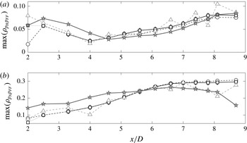
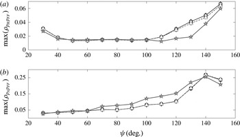
Taking advantage of the simultaneous measurements of near- and far-field pressures, a validation of the methods has been accomplished by computing the cross-correlation of the near-field separated pressure fields with the far-field pressure, that has to be considered as the measure of the actual acoustic pressure. The performance of the separation method is satisfactory if the correlation between near-field acoustic/hydrodynamic and far-field pressure is large/small. Figure 16 shows the axial evolution of the cross-correlation peak values of
 $p_{H}$
and
 $p_{A}$
with
 $p_{FF}$
at the polar position
 $\unicode[STIX]{x1D713}=140^{\circ }$
for Mach number
 $M_{j}=0.6$
. It can be seen that all the wavelet techniques perform satisfactorily since they provide large correlation between the far-field and the acoustic pressure whereas the one between the far-field and the hydrodynamic pressures is much smaller, the magnitude of the peaks being similar among all the procedures. A similar behaviour is observed also with respect to the reference
 $k-\unicode[STIX]{x1D714}$
technique but with some discrepancies. Specifically, for what concerns the acoustic pressure, it is found that for small axial distances the Fourier filtering technique provides cross-correlation peaks larger than those obtained by the wavelet-based methods. The opposite result is detected moving downstream in the jet. Such a behaviour can be ascribed to the different nature of the filtering bases, the wavelet one being more suited to detect large hydrodynamic fluctuations due to its better localization in the physical and transformed spaces. Figure 17 shows the polar evolution of the cross-correlation coefficient peak of the far-field pressure with the hydrodynamic and acoustic pressure components at the axial position
 $x/D=6.1$
. It is observed that a very good agreement between all the wavelet and the Fourier filtering techniques is detected for all the polar angles taken into account.
Axial evolution of the cross-correlation coefficient peak of near-field hydrodynamic and acoustic components with far-field pressure for polar position
 $\unicode[STIX]{x1D713}=140^{\circ }$
at
 $M_{j}=0.6$
. (a) Hydrodynamic component, (b) acoustic component. ♢ WT4, ○ WT1, ▵ WT2, ▫ WT3,
 $\star$
 $k-\unicode[STIX]{x1D714}$
technique.

Polar evolution of the cross-correlation coefficient peak of far-field pressure with near-field hydrodynamic and acoustic components at axial position
 $x/D=6.1$
at
 $M_{j}=0.6$
. (a) Hydrodynamic component, (b) acoustic component. ♢ WT4, ○ WT1, ▵ WT2, ▫ WT3,
 $\star$
 $k-\unicode[STIX]{x1D714}$
technique.

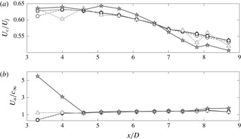
Finally the propagation velocities of the hydrodynamic and acoustic pressure fluctuations have been calculated based on the time delay associated with the cross-correlation peak between two consecutive streamwise near-field microphones. A standard procedure used in particle image velocimetry (PIV) data processing for the sub-pixel determination of the cross-correlation peak position has been used to improve the accuracy of the time delay position, thus reducing the associated bias error (Raffel et al.
Reference Raffel, Willert, Wereley and Kompenhans2007). Figure 18 shows the axial evolution of the normalized convection and sound propagation velocities at
 $M_{j}=0.6$
for all the separation techniques. It is observed that all the techniques provide equal velocity values. An exception for the acoustic propagation velocity obtained by the
 $k-\unicode[STIX]{x1D714}$
technique is found for axial positions close to the nozzle exhaust, the velocity values being much larger than the ambient speed of sound. Such discrepancy can be ascribed to the propagation direction of the sound waves parallel to the microphone array axis so that a phase velocity tending to infinite can be found in this region (Tinney & Jordan Reference Tinney and Jordan2008). It is interesting to underline that the convection velocity values found with the wavelet approaches for axial positions close to the nozzle exhaust are in very good agreement with results by Picard & Delville (Reference Picard and Delville2000) and Tinney & Jordan (Reference Tinney and Jordan2008).
Axial evolution of the normalized convection and acoustic propagation velocities for jet Mach number
 $M_{j}=0.6$
. (a) Convection velocity, (b) acoustic velocity. ♢ WT4, ○ WT1, ▵ WT2, ▫ WT3,
 $\star$
 $k-\unicode[STIX]{x1D714}$
technique.

4.3 Wavelet analysis of hydrodynamic and acoustic pressures
It has been shown above that all the proposed methods provide very similar results. Since the choice of the wavelet-based technique does not affect the resulting decomposition of the hydrodynamic and acoustic pressure fields, the physical features of the pseudo-sound and sound components shown below were derived by the application of the method WT1.
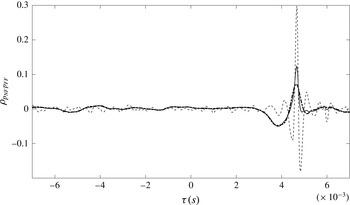
Figure 19 shows the cross-correlation coefficient of the near-field pressure signal and the separated hydrodynamic and acoustic components with the measured far-field pressure for
 $M_{j}=0.6$
. As a reference case, the near-field axial location
 $x/D=7.8$
was selected as well as the polar position
 $\unicode[STIX]{x1D713}=140^{\circ }$
for the far-field pressure. As expected, a large correlation between
 $p_{A}$
and
 $p_{FF}$
is found, whereas the correlation level between
 $p_{H}$
and
 $p_{FF}$
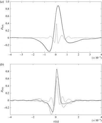
is almost negligible. It is important to underline that the amplitude of the correlation peak associated with the extracted acoustic component is considerably larger than the one related to the original near-field pressure signal. Such a behaviour is a proof that the radiating part of the near-field pressure has been properly isolated. This statement is further supported by the location of the acoustic–far-field pressure correlation peak, whose time delay leads to a propagation velocity of
 $345~\text{m}~\text{s}^{-1}$
, very close to the ambient speed of sound.
Wavelet technique WT1: cross-correlation coefficient of the original, hydrodynamic and acoustic near-field pressures at axial location
 $x/D=7.8$
with the far-field pressure at polar position
 $\unicode[STIX]{x1D713}=140^{\circ }$
for jet Mach number
 $M_{j}=0.6$
. Solid line corresponds to original pressure, dashed line to acoustic pressure, dash-dotted line to hydrodynamic pressure.

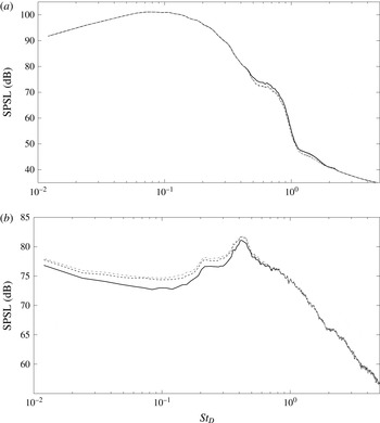
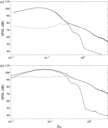
Figure 20 shows the SPSLs of the original pressure signal and the separated hydrodynamic and acoustic components for both jet Mach numbers for the same near-field position illustrated above. It is observed that the acoustic spectrum has a broadband energy distribution, whereas the spectral energy of the hydrodynamic component is concentrated at low–middle frequencies. For such frequency range the hydrodynamic pressure almost comprises all the energy level, conversely the acoustic pressure is larger at higher frequencies. The switch in the contribution to the global spectrum between
 $p_{H}$
and
 $p_{A}$
occurs close to the frequency where a change of the spectrum energy decay law is detected. Finally, it is noted that the contribution of the acoustic spectrum to the global spectral energy increases with increasing jet Mach number.
Wavelet technique WT1: SPSL of the original, hydrodynamic and acoustic pressure signals for a microphone axial position
 $x/D=7.8$
for both jet flow conditions. (a)
 $M_{j}=0.6$
, (b)
 $M_{j}=0.9$
. Solid line corresponds to original pressure, dashed line to acoustic pressure, dash-dotted line to hydrodynamic pressure.

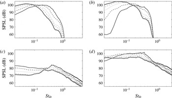
Figure 21 shows the axial evolution of the hydrodynamic and acoustic pressure spectra for both jet flow conditions at the microphone locations
 $x/D=3.3$
,
 $4.6$
,
 $6.1$
,
 $7.4$
,
 $8.7$
. The energy hump of the hydrodynamic contribution moves to low frequencies as the axial distance from the nozzle exhaust increases, such a behaviour being ascribed to the development of larger turbulent structures in the jet plume. It is interesting to underline that the increase of the Mach number does not considerably affect the amplitude of the pseudo-sound spectra. On the contrary, the amplitude of the acoustic spectra increases significantly for all the axial positions as the Mach number increases. According to Guitton et al. (Reference Guitton, Jordan, Laurendeau and Delville2007) and Grizzi & Camussi (Reference Grizzi and Camussi2012), such a result implies that the acoustic pressure is much more sensitive to the Mach number variation than the hydrodynamic component. It is also interesting to point out that, unlike the hydrodynamic pressure, the energy level of the acoustic component decreases moving downstream in the jet. Such a trend is in agreement with the results found in the literature (Grizzi & Camussi Reference Grizzi and Camussi2012).
Wavelet technique WT1: axial evolution of SPSLs of separated hydrodynamic and acoustic pressures for both jet flow conditions. (a) Hydrodynamic component,
 $M_{j}=0.6$
; (b) hydrodynamic component,
 $M_{j}=0.9$
; (c) acoustic component,
 $M_{j}=0.6$
; (d) acoustic component,
 $M_{j}=0.9$
. Solid lines
 $x/D=3.3$
, dashed lines
 $x/D=4.6$
, dotted lines
 $x/D=6.1$
, dash-dotted lines
 $x/D=7.4$
, bold lines
 $x/D=8.7$
.

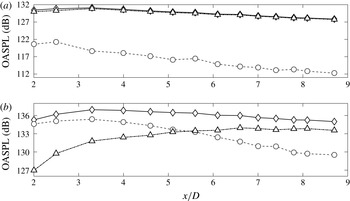
The physics described above is also confirmed by the axial evolution of the overall sound pressure level (OASPL) of the original, hydrodynamic and acoustic pressures for both jet flow conditions, as shown in figure 22. The OASPL was computed according to the following formula:
 $$\begin{eqnarray}\displaystyle \text{OASPL}=20\log _{10}\frac{\langle p^{\prime 2}\rangle ^{1/2}}{p_{ref}}. & & \displaystyle\end{eqnarray}$$
It can be observed that for
 $M_{j}=0.6$
the hydrodynamic component almost comprises the total noise level, whereas, as the jet Mach number increases, the contribution of the acoustic pressure to the total noise level increases significantly. It is evident that for
 $M_{j}=0.9$
the energy related to
 $p_{A}$
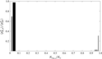
is larger close to the nozzle exhaust. Moving downstream, the contribution of the acoustic pressure decays very rapidly whereas the hydrodynamic contribution becomes more significant. A considerable result is shown in figure 23, in which the energy level of the hydrodynamic and acoustic pressures is represented against the number of the wavelet coefficients associated with each component. The wavelet coefficients number obtained from the wavelet transform of
 $p_{H}$
and
 $p_{A}$
is normalized by the total number of the coefficients. The variance of the two pressure components normalized by the variance of the original signal has been taken as an estimation of the overall relative energy associated with each contribution. It is observed that the hydrodynamic pressure almost comprises all the energy level with respect to the total energy amount and it is represented by a few but very intense wavelet coefficients. On the contrary, the acoustic pressure is characterized by a lower energy distributed on a much larger amount of wavelet coefficients. It is interesting to underline that the ratio between energy and wavelet coefficients number is a function of the jet Mach number. Specifically, it is observed that the energetic content of
 $p_{A}$
increases with the increasing Mach number, while the energy level related to
 $p_{H}$
falls off. Such a behaviour is in agreement with the experimental results shown so far.
Wavelet technique WT1: axial evolution of the OASPL of original, hydrodynamic and acoustic pressures for both jet flow conditions. (a)
 $M_{j}=0.6$
, (b)
 $M_{j}=0.9$
. ♢ original pressure, ○ acoustic pressure, ▵ hydrodynamic pressure.

Wavelet technique WT1: representation of the relative energy level of the separated hydrodynamic and acoustic pressure components function of the corresponding number of wavelet coefficients normalized by the total amount of wavelet coefficients. Black bars refer to hydrodynamic component, grey bars refer to acoustic components. Wide bars refer to
 $M_{j}=0.6$
, narrow bars refer to
 $M_{j}=0.9$
.

The different nature of
 $p_{H}$
and
 $p_{A}$
is further highlighted in figure 24, which shows the cross-correlation coefficient between two consecutive near-field pressure signals at axial positions
 $x/D=5.6$
and
 $x/D=6.1$
for both jet flow conditions. The hydrodynamic correlation is characterized by a larger time scale, the typical negative–positive bump shape being related to the signature of vortices convected by the jet flow. The time delay of the correlation peak is associated with a propagation velocity equal to
 $125~\text{m}~\text{s}^{-1}$
for
 $M_{j}=0.6$
and
 $186~\text{m}~\text{s}^{-1}$
for the case of
 $M_{j}=0.9$
, that is approximately
 $60$
% of the jet velocity, in agreement with Picard & Delville (Reference Picard and Delville2000) and Tinney & Jordan (Reference Tinney and Jordan2008). The acoustic counterpart shows a narrower and oscillatory correlation shape, very similar to the wave packet signature reported by Jordan & Colonius (Reference Jordan and Colonius2013). The peak delay is associated with propagation velocities respectively of
 $354~\text{m}~\text{s}^{-1}$
and
 $343~\text{m}~\text{s}^{-1}$
for the two jet Mach numbers analysed, these values being very close to the ambient speed of sound. It is also observed that the correlation between the pseudo-sound components almost coincides with the one between the original pressure signals. This result is related to the fact that the hydrodynamic pressure dominates in the near field. The correlation level between the acoustic pressures is found to be enhanced as the jet Mach number increases, such a behaviour being in agreement with the experimental results illustrated above.
Wavelet technique WT1: cross-correlation coefficient between two consecutive near-field microphone signals at axial positions
 $x/D=5.6$
and
 $x/D=6.1$
for both jet flow conditions: (a)
 $M_{j}=0.6$
, (b)
 $M_{j}=0.9$
. Solid lines correspond to original pressure, dashed lines to acoustic component, dash-dotted lines to hydrodynamic component.

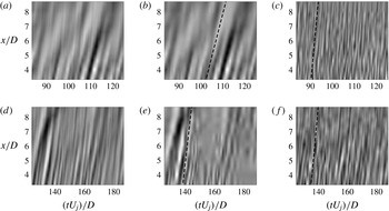
A global description of the near pressure field is provided in figure 25, in which the space–time contour map of
 $p_{NF}$
,
 $p_{H}$
and
 $p_{A}$
is shown for both jet Mach numbers. It is evident that the pressure fields obtained with the wavelet separation technique are quite similar to the ones derived from the
 $k-\unicode[STIX]{x1D714}$
technique shown in figure 13.
Wavelet technique WT1: space–time contour map of the original, the hydrodynamic and the acoustic near pressure fields. (a) Original pressure,
 $M_{j}=0.6$
; (b) hydrodynamic pressure,
 $M_{j}=0.6$
; (c) acoustic pressure,
 $M_{j}=0.6$
; (d) original pressure,
 $M_{j}=0.9$
; (e) hydrodynamic pressure,
 $M_{j}=0.9$
; (f) acoustic pressure,
 $M_{j}=0.9$
.

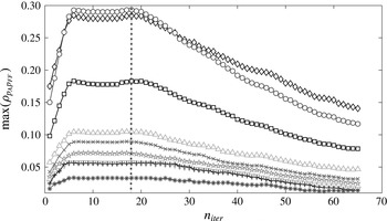
Wavelet technique WT1: trend of the cross-correlation coefficient peak along iterations between the near-field acoustic component and the far-field pressure measured at different polar angles. ♢
 $\unicode[STIX]{x1D713}=150^{\circ }$
, ○
 $\unicode[STIX]{x1D713}=140^{\circ }$
, ▫
 $\unicode[STIX]{x1D713}=130^{\circ }$
, ▵
 $\unicode[STIX]{x1D713}=120^{\circ }$
,
 $\times$
 $\unicode[STIX]{x1D713}=110^{\circ }$
,
 $\star$
 $\unicode[STIX]{x1D713}=100^{\circ }$
,
 ${\bigtriangledown}$
 $\unicode[STIX]{x1D713}=90^{\circ }$
,
 $+$
 $\unicode[STIX]{x1D713}=80^{\circ }$
,
 $\star$
 $\unicode[STIX]{x1D713}=50^{\circ }$
. The separation point for which the convergence criterion is satisfied is highlighted with a crossing dash-dotted line.

It is interesting to point out that the separation achieved with the method WT1 is not dependent on the position of the far-field microphone. This result is clearly described in figure 26, which shows the trend of the cross-correlation coefficient peak along the iterations between
 $p_{A}$
and
 $p_{FF}$
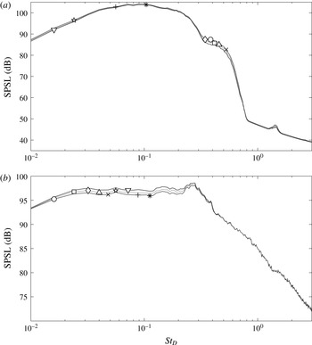
measured at different polar positions. Such a behaviour implies that whatever is the dominant noise component radiated in the far field, i.e. sound emissions from large turbulent structures or fine-scale turbulence, the separation procedure appears to be consistent. As a further test, figure 27 reports the hydrodynamic and acoustic pressure spectra showing the weak effect of the position in the far field, the maximum amplitude discrepancy being restricted to
 $1~\text{dB}$
without any modification of the spectral shape. The above results showed that the microphone far-field position does not affect the resulting separation so that the processing technique performs well across all the polar angles. Nevertheless, it has to be pointed out that the difference between the acoustic and hydrodynamic components in terms of correlation level with the far-field pressure shrinks as the polar angle decreases. Therefore a polar position of the far-field microphone in the aft arc, i.e.
 $\unicode[STIX]{x1D713}\geqslant 90^{\circ }$
, is recommended by the authors for the practical applications.
Wavelet technique WT1: effect of the far-field polar angle chosen to perform the separation on the hydrodynamic and acoustic pressure spectra at near-field axial location
 $x/D=6.6$
for jet Mach number
 $M_{j}=0.9$
. ♢
 $\unicode[STIX]{x1D713}=150^{\circ }$
, ○
 $\unicode[STIX]{x1D713}=140^{\circ }$
, ▫
 $\unicode[STIX]{x1D713}=130^{\circ }$
, ▵
 $\unicode[STIX]{x1D713}=120^{\circ }$
,
 $\times$
 $\unicode[STIX]{x1D713}=110^{\circ }$
,
 $\star$
 $\unicode[STIX]{x1D713}=100^{\circ }$
,
 ${\bigtriangledown}$
 $\unicode[STIX]{x1D713}=90^{\circ }$
,
 $+$
 $\unicode[STIX]{x1D713}=80^{\circ }$
,
 $\star$
 $\unicode[STIX]{x1D713}=50^{\circ }$
. (a) Hydrodynamic pressure, (b) acoustic pressure.

Wavelet technique WT1: axial evolution of the skewness factor of original, hydrodynamic and acoustic pressures for both jet conditions. (a)
 $M_{j}=0.6$
, (b)
 $M_{j}=0.9$
. ♢ original pressure, ○ acoustic component, ▵ hydrodynamic component.

Wavelet technique WT1: axial evolution of the flatness factor of original, hydrodynamic and acoustic pressures for both jet conditions. (a)
 $M_{j}=0.6$
, (b)
 $M_{j}=0.9$
. ♢ original pressure, ○ acoustic component, ▵ hydrodynamic component.

A statistical description of the near pressure field is further provided by the analysis of statistical moments and PDFs. Figure 28 shows the axial evolution of the skewness factor of
 $p_{NF}$
,
 $p_{H}$
and
 $p_{A}$
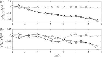
for both jet Mach numbers. It is observed that the skewness factor of
 $p_{H}$
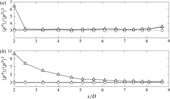
decreases moving downstream in the jet for both flow velocities as an effect of the turbulence development and almost coincides with that of the original pressure signal. On the contrary, the skewness of the acoustic component remains close to 0, as for the reference Gaussian distribution, for all the axial distances considered. Figure 29 reports the axial evolution of the dimensionless fourth-order statistical moment of the original, hydrodynamic and acoustic pressure signals for both flow velocities. It is observed that
 $p_{H}$
is characterized by very high values close to the nozzle exhaust; as the axial distance increases the flatness factor level reduces but remains larger than 3. The trend just described is more evident for the highest jet Mach number. On the contrary the
 $p_{A}$
flatness factor is equal to 3 for all the axial distances and velocities considered. The physics described highlights the different nature of the two pressure components in the near field: the hydrodynamic pressure is characterized by intermittent high-energy events, whereas the acoustic pressure has a nearly Gaussian nature. Such inference is further supported by the trend of the probability density functions. Figure 30 shows the axial evolution of the PDFs of the hydrodynamic and acoustic components for both jet Mach numbers at axial positions
 $x/D=3.3$
,
 $4.6$
,
 $6.1$
,
 $7.4$
,
 $8.7$
. Experimental PDFs are compared with a standard Gaussian distribution. It is observed that, unlike
 $p_{A}$
, the probability distribution of the hydrodynamic pressure deviates from the Gaussian one. For the case
 $M_{j}=0.6$
the PDFs of
 $p_{H}$
exhibits higher negative tails as the axial distance from the nozzle exhaust increases. This behaviour is related to the turbulence development and the generation of intermittent peaks of vorticity associated with large pressure drops (Abry et al.
Reference Abry, Fauve, Flandrin and Laroche1994; Grizzi & Camussi Reference Grizzi and Camussi2012).
Wavelet technique WT1: axial evolution of the probability density functions of the hydrodynamic and acoustic pressures for both jet Mach numbers. (a) Hydrodynamic component,
 $M_{j}=0.6$
; (b) hydrodynamic component,
 $M_{j}=0.9$
; (c) acoustic component,
 $M_{j}=0.6$
; (d) acoustic component,
 $M_{j}=0.9$
. ♢
 $x/D=3.3$
, ○
 $x/D=4.6$
, ▫
 $x/D=6.1$
, ▵
 $x/D=7.4$
,
 $\star$
 $x/D=8.7$
. Dashed line refers to the standard Gaussian distribution.

5 Conclusions
In the present work three novel signal processing techniques based on wavelet transform providing the decomposition of the near pressure field of a jet into hydrodynamic and acoustic components are introduced and validated. An experimental database involving simultaneous near- and far-field measurements of pressure fluctuations was exploited to derive the innovative methods. The experimental investigation was carried out on a single-stream jet at high Reynolds numbers and for two Mach numbers available in the anechoic wind tunnel of the Centre Acoustique of Laboratoire de Mécanique des Fluides et d’Acoustique at the École Centrale de Lyon. Preliminary aerodynamic and aeroacoustic qualifications of the jet were provided in terms of main statistical quantities, spectral content, cross-correlation trend and noise levels in the near field as well as in the far field.
The experimental results obtained by the application of the novel techniques were compared with the outcome provided by two further separation procedures found in the literature. The first one is a Fourier filtering technique in which the hydrodynamic and acoustic pressures are extracted based on their phase velocity in the wavenumber–frequency spectrum. The second technique is a wavelet-based procedure in which pseudo-sound and sound components are extracted from a pair of near-field pressure signals by a proper thresholding procedure.
The improvement of the efficiency of the latter method aimed at a further simplification of the set-up required to perform the hydrodynamic/acoustic pressure decomposition as well as a better understanding of the jet noise physics motivated the present work. The choice of the above-mentioned threshold was achieved establishing different convergence criteria based on the intrinsic nature of the hydrodynamic and acoustic pressures.
-
(i) In the wavelet technique WT1 one near-field and one far-field microphone acquiring simultaneously are required to perform the separation. The assumption underlying this procedure is that the acoustic component in the near field is associated with the pressure fluctuations destined to reach the far field. Whereas the hydrodynamic component is characterized by a very rapid decay as the radial distance from the jet axis increases. The pseudo-sound and sound components were iteratively separated until the cross-correlation peak between the near-field acoustic pressure and the far-field pressure reached a maximum. It has been shown that the choice of the polar position of the far-field microphone used to perform the separation does not affect the decomposition of the hydrodynamic and acoustic pressures. Such a result means that the separation is not dependent on the dominant noise component in the far field, i.e. large/fine-scale turbulent structures in the aft/forward arc.
-
(ii) Based on the statistical analysis of the far-field pressure, a separation technique requiring only one microphone in the near field was developed. The assumption underlying the technique WT2 is the nearly Gaussian nature of the acoustic pressure. The hydrodynamic and acoustic pressures were iteratively separated until the difference between the PDF of the sound component and the standard Gaussian distribution was lower than a tolerance value.
-
(iii) Based on the assumption that the hydrodynamic component is related to pressure fluctuations induced by localized coherent turbulent structures and on account of the relation between hydrodynamic pressure and vorticity, a wavelet technique used to extract the coherent structures of the vorticity field has been applied to the pressure data. In the wavelet technique WT3 the pseudo-sound and sound components were iteratively separated until the number of the wavelet coefficients related to the acoustic pressure became constant.
The proposed methods were validated against the reference separation techniques, highlighting that all the wavelet-based procedures led to very similar results.
The hydrodynamic and acoustic pressure fields have been analysed in the time and frequency domain in order to provide a statistical and spectral characterization. The axial evolution of the pseudo-sound and sound components has been described as well as the effect of the jet Mach number on the two pressure fields. Specifically the spectral energy of the hydrodynamic pressure was found to rise as the axial distance increased. On the contrary, the energy content associated with the acoustic pressure was found to be higher for axial positions close to the nozzle exhaust. Unlike the hydrodynamic pressure spectra, the amplitude of the acoustic pressure spectra was strongly affected by the jet Mach number, the noise level being significantly enhanced for the highest jet velocity. Such a behaviour was also confirmed by the OASPL trends. The different characteristics of the two pressure components were highlighted by the cross-correlation trend between two consecutive near-field microphone signals. The hydrodynamic pressure was characterized by a typical negative–positive bump shape with a large time scale related to the vortex convection. The acoustic pressure showed a narrower correlation with an oscillatory trend, its peak time delay being related to a propagation velocity of the order of the speed of sound. The different nature of the two pressure components also arose from the axial evolution of the third- and fourth-order statistical moments and of the probability density function distributions. Such results shed light on the intermittent and nearly Gaussian nature of the hydrodynamic and acoustic pressures respectively.
Finally, with the intention of performing the hydrodynamic and acoustic pressure separation, it has to be pointed out that the
 $k-\unicode[STIX]{x1D714}$
technique requires a large microphone array in order to have an acceptable resolution in the wave-number domain. On the contrary the wavelet techniques proposed require a very simple set-up consisting of two microphones at most: one in the near field and one in the far field. Therefore, these methods can be easily applied to pressure signals (e.g. obtained by wind tunnel measurements) as an important device to filter out the hydrodynamic component induced by the jet flow and retain just the pressure fluctuations related to sound emissions. This aspect could be relevant, for instance, when using noise sources detection algorithm such as the beamforming technique in order to have a better identification of noise sources location and level.
The simplicity of the required set-up to perform the hydrodynamic/acoustic separation makes the proposed methods (especially the ones based on one microphone in the near field) attractive for a large variety of engineering applications, such as jet noise control and wall-bounded flows. Indeed, the separation between the acoustic component and the hydrodynamic counterpart could be likely achieved in the case of turbulent boundary layers. Such feature could be essential to develop improved prediction models for the vibrations transmitted through the surface (e.g. the interior noise transmitted to the aircraft/car cockpit). Indeed, this application is a task currently underway by the authors.
Future developments of the approach presented in this manuscript could concern the application of the wavelet-based procedures to pressure field data obtained by a wave packet source in order to prove the separation techniques with a modelled pressure field.
Furthermore it has to be underlined that, unlike both the reference methods found in the literature, the separation achieved with the techniques proposed herein is not based on the propagation velocity of the two contributions. Hence, the present techniques could be used to separate hydrodynamic and acoustic pressures also in near-sonic and supersonic conditions.
Acknowledgements
The authors acknowledge the support of the EU Collaborative project ORINOCO (ACP0-GA-2010-266103). M.M. and R.C. also acknowledge the partial support of the EU Collaborative project JERONIMO (ACP2-GA-2012-314692). Both the projects are funded under the 7th Framework Program. Olivier Léon is acknowledged for his work during the experimental test campaign.