1. Introduction
Gas–liquid flows are important in a variety of physical and technological settings, ranging from the shearing of water layers in oceans to the flow of hydrocarbons in oil pipelines. For example, in the transport of high-viscosity crude oil through long-distance pipelines using a core–annular flow technique, a thin water film is introduced to surround the inner oil core, with the waves on the oil–water interface playing a crucial role in determining the stability of the two-liquid layer. Other engineering systems that utilise gas–liquid flows include distillation, absorption and the cooling of electronic devices. An accurate description and fundamental understanding of the spatiotemporal evolution of two-fluid interfaces and the associated wave formation processes is crucial for the design and optimisation of processes and devices that exploit two-fluid interfaces.
Thin liquid films flowing over inclined plates have been the subject of many studies since the first experiments of Kapitza (Reference Kapitza and Ter Haar1948). This apparently simple system exhibits a rich dynamical behaviour starting with a flat film that undergoes a series of bifurcations eventually ending in spatiotemporal chaos. For small values of the liquid flow rate, the free surface is fundamentally two-dimensional, consisting of single-hump solitary waves that are formed as a result of the primary wavefield undergoing a secondary instability. Such solitary waves are observed in a number of theoretical (Chang, Demekhin & Kalaidin Reference Chang, Demekhin and Kalaidin1995; Malamataris & Balakotaiah Reference Malamataris and Balakotaiah2008) and experimental studies (Liu & Gollub Reference Liu and Gollub1994; Vlachogiannis & Bontozoglou Reference Vlachogiannis and Bontozoglou2001). For extensive reviews of falling liquid film studies, the reader is referred to the monographs by Alekseenko, Nakoryakov & Pokusaev (Reference Alekseenko, Nakoryakov and Pokusaev1994), Chang & Demekhin (Reference Chang and Demekhin2002) and Kalliadasis et al. (Reference Kalliadasis, Ruyer-Quil, Scheid and Velarde2012).
The addition of a gas layer to the liquid film makes the system dynamics even more complex and interesting. This results in a number of flow regimes such as bubbly flow, slug flow, wavy flow, churn flow and annular flow, to name a few (Azzopardi Reference Azzopardi2006). Due to a number of applications and the intriguing underlying physics, gas–liquid flows have remained an active topic of research for more than six decades. Hanratty & Engen (Reference Hanratty and Engen1957) were among the first to analyse stratified gas–liquid flows. These authors investigated the co-current flow of an air–water system, and showed various wave transitions through their experiments. Craik (Reference Craik1966) studied thin water films in a horizontal channel experimentally, and reported the presence of fast and slow waves, which travelled faster and slower than the interface, respectively. When the gas velocity is increased beyond a particular value, it results in the formation of roll waves at the interface, which is a signature of droplet entrainment into the gas stream (Woodmansee & Hanratty Reference Woodmansee and Hanratty1969). Demekhin (Reference Demekhin1981) and Trifonov (Reference Trifonov2010) analysed the vertical gas–liquid problem by following the quasi-laminar approach of Benjamin (Reference Benjamin1957) and Miles (Reference Miles1957). Moreover, Trifonov (Reference Trifonov2010) solved the full Navier–Stokes equations for the liquid problem, whereas Demekhin (Reference Demekhin1981) developed an integral-boundary-layer model. Recently, Ó Náraigh, Spelt & Zaki (Reference Ó Náraigh, Spelt and Zaki2011) considered turbulent flow over a liquid layer by developing a single-equation model for the interfacial turbulence. By solving the full two-phase flow problem for the horizontal configuration and on comparison with various models such as the simple quasi-laminar model, eddy viscosity model, visco-elastic model and rapid distortion theory, they concluded that the waviness-induced Reynolds stresses do not play a significant role in determining the stability of the interface. Tseluiko & Kalliadasis (Reference Tseluiko and Kalliadasis2011) solved the counter-current gas–liquid problem by using an improved version of the quasi-laminar approach of Benjamin (Reference Benjamin1957) and Miles (Reference Miles1957). However, their analysis of the gas problem was performed using a curvilinear boundary-layer coordinate system, which gives significantly better agreement with experiments, unlike the solution to the gas problem using a Cartesian coordinate system by Demekhin (Reference Demekhin1981) and Trifonov (Reference Trifonov2010). Further, Tseluiko & Kalliadasis (Reference Tseluiko and Kalliadasis2011) developed non-local long-wave (LW) and weighted integral-boundary-layer (WIBL) models for the liquid problem to investigate the phenomenon of ‘flooding’, which corresponds to the appearance of large-amplitude standing waves. A weakly nonlinear non-local model obtained by assuming small-amplitude waves was analysed in Lin, Tseluiko & Kalliadasis (Reference Lin, Tseluiko and Kalliadasis2014). In the co-current version of the problem, the nonlinear wave speed was found to increase with increase in the gas shear and the liquid flow rate (Vellingiri et al. Reference Vellingiri, Tseluiko, Savva and Kalliadasis2013).
Miesen & Boersma (Reference Miesen and Boersma1995) analysed the stability of a vertical thin liquid film sheared by a co-flowing turbulent gas. By considering the dynamic effects of the gas, they found two modes of instability, namely the interfacial mode and the internal mode. The interfacial mode has a phase speed larger than the maximum velocity in the liquid layer, whereas the phase speed of the internal mode is smaller than the maximum velocity in the liquid film. They also compared their model calculations with experiments, and they tried to link the generation of roll waves with droplet entrainment. In another study, Boomkamp & Miesen (Reference Boomkamp and Miesen1996) provided a general classification of instabilities in parallel two-phase flows based on the energy transfer from the primary to the disturbed flow. They classified the existing studies on such instabilities into five different groups, based on the mechanism of energy transfer, which in turn depends on the properties of the flow system, namely density stratification and orientation, curvature of the velocity profile, viscosity stratification, shear effects or a combination of the last two. Camassa et al. (Reference Camassa, Forest, Lee, Ogrosky and Olander2012) performed experiments on a vertical core–annular flow system, where a thin liquid film lining the inside of a circular tube is driven by a counter-current turbulent air flow. They also compared their experimental results with a simple LW model. Finally, in a recent study, Dietze & Ruyer-Quil (Reference Dietze and Ruyer-Quil2013) considered a thin liquid film in the presence of a confined laminar gas for both horizontal and vertical configurations. By making use of the laminar nature of the flow, they developed a model based on the WIBL approach for both phases, also taking into account the viscous diffusion effects.
In the present study, we are interested in analysing absolute and convective instabilities in a gas–liquid flow system, where a thin liquid film flowing down an inclined wall is in contact with a counter-current turbulent gas flow. According to some of the earlier studies (Shearer & Davidson Reference Shearer and Davidson1965; Cetinbudaklar & Jameson Reference Cetinbudaklar and Jameson1969), the flooding point corresponds to the critical gas flow rate where a standing wave is formed on the interface, whose amplitude is much larger than the mean film thickness. We further propose that this critical gas flow rate indeed has a close correspondence with the onset of absolute instability in the system. The absolute instability allows the disturbances to grow at fixed points in space and therefore results in large-amplitude waves that are not necessarily convected downstream or upstream. The theory of absolute and convective instabilities was first introduced in the field of plasma physics (Briggs Reference Briggs1964), and was later developed in fluid dynamics (Huerre & Monkewitz Reference Huerre and Monkewitz1990; Huerre Reference Huerre, Batchelor, Moffatt and Worster2000). Absolute and convective instabilities are found in a variety of fluid flow settings such as liquid sheets and jets (Lin Reference Lin2003), combustion (Juniper Reference Juniper2006) and many other flow processes. These instabilities are also analysed from a more dynamical system perspective, using, e.g. the complex Ginzburg–Landau equation (Chaté & Manneville Reference Chaté and Manneville1996; Tobias, Proctor & Knobloch Reference Tobias, Proctor and Knobloch1998), a generic model system for a variety of physical systems close to the instability threshold.
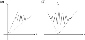
In general, the nature of the instability is determined by examining the response of the linear system to a localised disturbance. If the growing disturbance gets advected and moves away from the point of initiation, then the instability is convective. In other words, if the long-time behaviour of the system decays along the ray
 $x/t=0$
, then the system is said to be convectively unstable (see figure 1). On the other hand, if the disturbance grows at every point in space, then the instability is absolute. Convectively unstable flows are also referred to as ‘spatial amplifiers’, whereas absolutely unstable flows act like ‘oscillators’ (Huerre Reference Huerre, Batchelor, Moffatt and Worster2000; Duprat et al.
Reference Duprat, Ruyer-Quil, Kalliadasis and Giorgiutti-Dauphiné2007). Gaster (Reference Gaster1962) demonstrated that the spatial growth rate could be obtained from the temporal one through an appropriate transformation, but such a transformation is applicable only for near-critical conditions.
Schematic representation of (a) convective and (b) absolute instabilities.

Brevdo et al. (Reference Brevdo, Laure, Dias and Bridges1999) were among the first to analyse absolute and convective instabilities in a falling film setting by solving the associated Orr–Sommerfeld (OS) problem. These authors considered two different techniques to analyse absolute and convective instabilities, one based on the exact Briggs collision criterion and the other based on the tracking of the saddle point, which provides the leading-order contribution to the inverse Fourier and Laplace transforms. However, they found only a convective instability from their numerical studies, as expected. Suslov (Reference Suslov2006) developed a more complicated algorithm to compute the absolute–convective stability boundary in the given parameter space. Joo & Davis (Reference Joo and Davis1992) analysed instabilities in a falling film using Benney’s LW evolution equation, and confirmed that the instability is of the convective type. A detailed analysis of the linear stability characteristics of a falling film is given in Kalliadasis et al. (Reference Kalliadasis, Ruyer-Quil, Scheid and Velarde2012). Lin & Kondic (Reference Lin and Kondic2010) also considered absolute–convective instabilities in their study on thin film flows on inverted substrates. In a very recent study, Ó Náraigh, Spelt & Shaw (Reference Ó Náraigh, Spelt and Shaw2013) analysed absolute and convective instabilities of a horizontal thin liquid film sheared by a fully developed gas flow that could be laminar or turbulent. By combining linear modal and ray analyses, they calculated the regimes of such instabilities and they also found that absolute instability exists for large values of density and viscosity ratios at high Reynolds numbers. To model the turbulent gas flow, they used a simple quasi-laminar assumption where the turbulence contribution enters solely through the base velocity profile, thereby ignoring waviness-induced Reynolds stresses. Although Ó Náraigh et al. (Reference Ó Náraigh, Spelt and Zaki2011, Reference Ó Náraigh, Spelt and Shaw2013) found that the waviness-induced Reynolds stresses do not play a significant role in the stability of the interface for the parameter values they considered, it should be noted that the simple quasi-laminar assumption does not provide good agreement with experiments – e.g. by Thorsness, Morrisroe & Hanratty (Reference Thorsness, Morrisroe and Hanratty1978) – as shown in Tseluiko & Kalliadasis (Reference Tseluiko and Kalliadasis2011). Moreover, the conclusion of Ó Náraigh et al. (Reference Ó Náraigh, Spelt and Zaki2011, Reference Ó Náraigh, Spelt and Shaw2013) on the impact of waviness-induced Reynolds stresses on the interfacial instability seems to be in contradiction to the results presented in Tseluiko & Kalliadasis (Reference Tseluiko and Kalliadasis2011). Therefore, an improved version of the quasi-laminar assumption needs to be used, as in Tseluiko & Kalliadasis (Reference Tseluiko and Kalliadasis2011). From the modelling point of view, the fact that Ó Náraigh et al. (Reference Ó Náraigh, Spelt and Zaki2011, Reference Ó Náraigh, Spelt and Shaw2013) assume that the turbulence enters only through the base velocity results in a linearised problem that completely ignores the turbulent Reynolds stresses, i.e. it follows that the Reynolds-averaged Navier–Stokes equations are used to obtain the base velocity profile, but the usual Navier–Stokes equations are used for the stability analysis – this is an inconsistency in the sense that the base velocity profile does not satisfy the equations used for the stability analysis. In our approach this inconsistency is avoided. From the mathematical point of view, our approach leads to non-local equations, whereas the equations of Ó Náraigh et al. (Reference Ó Náraigh, Spelt and Shaw2013) are local. This means that the standard absolute/convective instability analysis (see, e.g. Huerre & Monkewitz Reference Huerre and Monkewitz1990) is not applicable to our situation, and we therefore devise a generalised methodology for analysing absolute/convective instabilities.
Our linear stability analysis begins with the formulation of a modified OS equation for the vertically falling liquid problem incorporating the effects of counter-current gas flow. As mentioned earlier, in a recent study Tseluiko & Kalliadasis (Reference Tseluiko and Kalliadasis2011) developed a hierarchy of non-local low-dimensional models, namely an LW model and a WIBL model, to analyse flooding in counter-current gas–liquid flows, focusing mainly on single-hump solitary waves and periodic travelling waves. Their WIBL model is based on the methodology of Ruyer-Quil & Manneville (Reference Ruyer-Quil and Manneville1998, Reference Ruyer-Quil and Manneville2000) for falling liquid films, obtained by combining an LW expansion with a polynomial representation of the velocity field, with the integral-boundary-layer approximation and the method of weighted residuals. The advantage with the WIBL model is that it can be applied up to moderate Reynolds numbers. This methodology, appropriately modified, has been applied successfully on falling films in the presence of various complexities, i.e. wall curvature effects (Ruyer-Quil et al. Reference Ruyer-Quil, Treveleyan, Giorgiutti-Dauphiné, Duprat and Kalliadasis2008; Ruyer-Quil & Kalliadasis Reference Ruyer-Quil and Kalliadasis2012), thermocapillary Marangoni effects (Trevelyan & Kalliadasis Reference Trevelyan and Kalliadasis2004a ,Reference Trevelyan and Kalliadasis b ; Ruyer-Quil et al. Reference Ruyer-Quil, Scheid, Kalliadasis, Velarde and Zeytounian2005; Trevelyan et al. Reference Trevelyan, Scheid, Ruyer-Quil and Kalliadasis2007) and the solutal Marangoni effect (Pereira & Kalliadasis Reference Pereira and Kalliadasis2008). Although it is known that generally WIBL models perform significantly better than Benney-type LW models and are valid up to moderate values of the Reynolds number, to truly analyse the range of validity of such LW models in any particular set-up, it is important to compare their predictions with, e.g. experiments or the full equations. The present study is an important step towards such validation. Namely, we perform the linear stability analysis and absolute/convective stability analysis for both the full equations and the reduced models and compare their results.
In § 2 we present the governing equations and the dimensionless parameters. In § 3 we recall the low-dimensional models of Tseluiko & Kalliadasis (Reference Tseluiko and Kalliadasis2011). In § 4 we derive the modified OS equation from the Navier–Stokes equations and the associated boundary conditions, and derive the linearised versions for the reduced model equations. By assuming normal mode solutions, we then examine the temporal stability of the system in § 5.1, and in § 5.2 we perform an energy analysis to elucidate the physical nature of the instability. In § 5.3 we devise a methodology to analyse absolute–convective instabilities. The linear stability results are supplemented by time-dependent computations of the linearised WIBL model in § 5.4. Finally, we summarise our findings in § 6.
2. Problem formulation
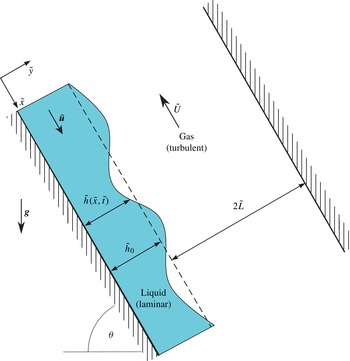
Our prototypical system consists of a two-dimensional channel that is inclined at an angle
 ${\it\theta}$
with respect to the horizontal, as depicted in figure 2. A thin liquid film of density
 ${\it\rho}_{\ell }$
and viscosity
 ${\it\mu}_{\ell }$
flows along the bottom wall of the channel due to gravity. The rest of the channel is occupied by an upflowing gas, which has density
 ${\it\rho}_{g}$
and viscosity
 ${\it\mu}_{g}$
. The liquid film is taken to be laminar, whereas the gas flow is considered to be turbulent. We introduce a Cartesian coordinate system
 $(\tilde{x},{\tilde{y}})$
with the
 $\tilde{x}$
-axis pointing along the lower wall and the
 ${\tilde{y}}$
-axis pointing into the liquid film. Tildes denote dimensional variables. The interface is located at
 ${\tilde{y}}=\tilde{h}(\tilde{x},\tilde{t})$
, where
 $\tilde{t}$
denotes time. The undisturbed film thickness is denoted by
 $\tilde{h}_{0}$
and the distance between the undisturbed interface and the upper wall is denoted by
 $2\tilde{L}$
.
Schematic illustration of a falling liquid film in contact with a counter-current turbulent gas. Here,
 ${\it\theta}$
is the inclination angle of the channel with respect to the horizontal.

The governing equations for the liquid problem are the Navier–Stokes equations:
 $$\begin{eqnarray}\displaystyle & {\it\rho}_{\ell }\left(\tilde{\boldsymbol{u}}_{\tilde{t}}+\tilde{\boldsymbol{u}}\boldsymbol{\cdot }\boldsymbol{{\rm\nabla}}\tilde{\boldsymbol{u}}\right)=-\boldsymbol{{\rm\nabla}}\tilde{p}+{\it\mu}_{\ell }{\rm\nabla}^{2}\tilde{\boldsymbol{u}}+{\it\rho}_{\ell }\boldsymbol{g}, & \displaystyle\end{eqnarray}$$
 $$\begin{eqnarray}\displaystyle & \boldsymbol{{\rm\nabla}}\boldsymbol{\cdot }\tilde{\boldsymbol{u}}=0, & \displaystyle\end{eqnarray}$$
 $\tilde{\boldsymbol{u}}=(\tilde{u} ,\tilde{v})$
is the liquid velocity,
 $\tilde{p}$
is the pressure and
 $\boldsymbol{g}=(g\sin {\it\theta},-g\cos {\it\theta})$
, with
 $g$
denoting the acceleration due to gravity. The no-slip and no-penetration conditions at the bottom wall imply
 $$\begin{eqnarray}\tilde{\boldsymbol{u}}=\mathbf{0}\quad \text{at}~{\tilde{y}}=0.\end{eqnarray}$$
The kinematic condition at the gas–liquid interface
 $\tilde{h}$
is
 $$\begin{eqnarray}\tilde{h}_{\tilde{t}}+\tilde{u} \tilde{h}_{\tilde{x}}=\tilde{v}\quad \text{at}~{\tilde{y}}=\tilde{h}(\tilde{x},\tilde{t}).\end{eqnarray}$$
The tangential stress balance is given by
 $$\begin{eqnarray}-{\displaystyle \frac{{\it\mu}_{\ell }}{1+\tilde{h}_{\tilde{x}}^{2}}}[2(\tilde{u} _{\tilde{x}}-\tilde{v}_{{\tilde{y}}})-(\tilde{u} _{{\tilde{y}}}+\tilde{v}_{\tilde{x}})(1-\tilde{h}_{\tilde{x}}^{2})]=\tilde{{\it\tau}}_{w}[\tilde{h}]\quad \text{at}~{\tilde{y}}=\tilde{h}(\tilde{x},\tilde{t}),\end{eqnarray}$$
where
 $\tilde{{\it\tau}}_{w}[\tilde{h}]$
is the tangential stress at the interface due to the turbulent gas flow. The normal stress balance can be written as
 $$\begin{eqnarray}\tilde{p}=\tilde{P}_{w}[\tilde{h}]+{\displaystyle \frac{2{\it\mu}_{\ell }}{1+\tilde{h}_{\tilde{x}}^{2}}}[\tilde{u} _{\tilde{x}}\tilde{h}_{\tilde{x}}^{2}-(\tilde{u} _{{\tilde{y}}}+\tilde{v}_{\tilde{x}})\tilde{h}_{\tilde{x}}+\tilde{v}_{{\tilde{y}}}]-{\displaystyle \frac{{\it\sigma}\tilde{h}_{\tilde{x}\tilde{x}}}{(1+\tilde{h}_{\tilde{x}}^{2})^{3/2}}}\quad \text{at}~{\tilde{y}}=\tilde{h}(\tilde{x},\tilde{t}),\end{eqnarray}$$
where
 $\tilde{P}_{w}[\tilde{h}]$
is the pressure exerted at the interface by the turbulent gas. Expressions for the tangential and normal stresses exerted by the turbulent gas on the liquid film have been obtained by Tseluiko & Kalliadasis (Reference Tseluiko and Kalliadasis2011) and turn out to be non-local operators of the interface shape. These expressions will be given below in dimensionless forms. The basic hypotheses by Tseluiko & Kalliadasis (Reference Tseluiko and Kalliadasis2011) are that the dynamic viscosity of the gas is much smaller than that of the liquid, that the typical velocity in the liquid and that of the interfacial waves are much smaller than the typical velocity of the gas and that of a ‘linear response’, i.e. the interface, written as a superposition of Fourier harmonics of wavenumber say
 ${\it\alpha}_{n}$
(assuming periodicity), induces tangential and normal stresses which are also superpositions of Fourier harmonics of the same wavenumber
 ${\it\alpha}_{n}$
. In choosing the turbulence model, the motivation of Tseluiko & Kalliadasis (Reference Tseluiko and Kalliadasis2011) was to utilise a simple model that gives good agreement with experiments and allows for analytical progress to be made with the problem. Therefore, Tseluiko & Kalliadasis (Reference Tseluiko and Kalliadasis2011) used Prandtl’s mixing length theory with the mixing length modelled by the van Driest equation. The drawbacks of this mixing length model are well known (e.g. it predicts that the apparent viscosity should vanish in the middle of the channel, which is actually not the case); however, it still provides good agreement with experiments in many situations (e.g. Schlichting Reference Schlichting2000). To model turbulent flow over a wavy surface, Tseluiko & Kalliadasis (Reference Tseluiko and Kalliadasis2011) chose to work in orthogonal boundary-layer coordinates introduced by Benjamin (Reference Benjamin1959), in which to leading order the wall coincides with a coordinate line and far from the wall the coordinate lines of the curvilinear system approach exponentially those of the Cartesian system. Tseluiko & Kalliadasis (Reference Tseluiko and Kalliadasis2011) assumed that the waviness-induced turbulent Reynolds stresses vanish in such coordinates (which implicitly provides a model for the waviness-induced Reynolds stresses in Cartesian coordinates) and demonstrated by comparing with experimental results presented in Thorsness et al. (Reference Thorsness, Morrisroe and Hanratty1978) that such modelling is capable of capturing satisfactorily the effects of turbulent gas flow over a wavy surface (see figures 5–11 in Tseluiko & Kalliadasis Reference Tseluiko and Kalliadasis2011).
To make the above equations dimensionless, we choose the following scales for length (
 $l_{c}$
), velocity (
 $\tilde{u} _{c}$
), time (
 $\tilde{t}_{c}$
) and pressure (
 $\tilde{p}_{c}$
):
 $$\begin{eqnarray}\tilde{l}_{c}=\tilde{h}_{0};\quad \tilde{u} _{c}={\displaystyle \frac{{\it\rho}_{\ell }g\tilde{h}_{0}^{2}\sin {\it\theta}}{2{\it\mu}_{\ell }}};\quad \tilde{t}_{c}={\displaystyle \frac{\tilde{h}_{0}}{\tilde{u} _{c}}};\quad \tilde{p}_{c}={\displaystyle \frac{{\it\mu}_{\ell }\tilde{u} _{c}}{\tilde{h}_{0}}}.\end{eqnarray}$$
Using these, the Navier–Stokes equations are written in dimensionless form as follows:
 $$\begin{eqnarray}\displaystyle & \mathit{Re}\left(u_{t}+uu_{x}+vu_{y}\right)=-p_{x}+u_{xx}+u_{yy}+2, & \displaystyle\end{eqnarray}$$
 $$\begin{eqnarray}\displaystyle & \mathit{Re}\left(v_{t}+uv_{x}+vv_{y}\right)=-p_{y}+v_{xx}+v_{yy}-2\cot {\it\theta}, & \displaystyle\end{eqnarray}$$
 $$\begin{eqnarray}\displaystyle & u_{x}+v_{y}=0, & \displaystyle\end{eqnarray}$$
 $$\begin{eqnarray}\mathit{Re}=\frac{{\it\rho}_{\ell }^{2}g\tilde{h}_{0}^{3}\sin {\it\theta}}{2{\it\mu}_{\ell }^{2}}\end{eqnarray}$$
is the Reynolds number. At the bottom wall, we have
 $$\begin{eqnarray}u=v=0,\quad \text{at}~y=0.\end{eqnarray}$$
On the interface, the dimensionless kinematic condition is given by
 $$\begin{eqnarray}h_{t}+uh_{x}=v,\quad \text{at}~y=h(x,t),\end{eqnarray}$$
with the dimensionless tangential stress condition given by
 $$\begin{eqnarray}-\frac{1}{1+h_{x}^{2}}[2(u_{x}-v_{y})h_{x}-(u_{y}+v_{x})(1-h_{x}^{2})]=\hat{{\it\tau}}_{w}[h]\quad \text{at}~y=h(x,t).\end{eqnarray}$$
Here,
 $$\begin{eqnarray}\hat{{\it\tau}}_{w}[h]=\hat{{\it\tau}}_{w0}+\hat{{\it\tau}}_{w0}{\it\nu}\hspace{2.22198pt}\hat{{\it\tau}}_{w1}[h],\end{eqnarray}$$
with
 $$\begin{eqnarray}\hat{{\it\tau}}_{w0}=\frac{\tilde{h}_{0}T_{w}{\it\tau}_{w0}}{{\it\mu}_{l}\tilde{u} _{0}},\quad {\it\nu}=\frac{\tilde{h}_{0}{\it\rho}_{g}U_{f}^{\ast }}{{\it\mu}_{g}},\quad \hat{{\it\tau}}_{w1}[h]\equiv \mathop{\sum }_{\begin{array}{@{}c@{}}n=-\infty \\ n\neq 0\end{array}}^{\infty }h_{n}{{\it\tau}_{w}}_{1}({\it\alpha}_{n}/{\it\nu})\text{e}^{\text{i}{\it\alpha}_{n}x},\end{eqnarray}$$
where
 $U_{f}^{\ast }$
is the frictional velocity in the turbulent gas flow, and
 ${\it\alpha}_{n}$
is the wavenumber. The dimensionless form of the normal stress balance condition can be written as
 $$\begin{eqnarray}p=\widehat{P}_{w}[h]+\frac{2}{1+h_{x}^{2}}[u_{x}h_{x}^{2}-(u_{y}+v_{x})h_{x}+v_{y}]-\frac{\mathit{Re}\,\mathit{We}\,h_{xx}}{(1+h_{x}^{2})^{3/2}},\quad \text{at}~y=h(x,t),\end{eqnarray}$$
where
 $$\begin{eqnarray}\widehat{P}_{w}[h]=\widehat{P}_{0}+|\hat{{\it\tau}}_{w0}|{\it\nu}\widehat{P}_{1}[h],\end{eqnarray}$$
 $$\begin{eqnarray}\widehat{P}_{0}=|\hat{{\it\tau}}_{w0}|P_{0}={\widehat{P}_{0}}^{a}+{\widehat{P}_{0}}^{b}x,\quad \widehat{P}_{1}[h]\equiv \mathop{\sum }_{\begin{array}{@{}c@{}}n=-\infty \\ n\neq 0\end{array}}^{\infty }h_{n}{P_{w}}_{1}({\it\alpha}_{n}/{\it\nu})\text{e}^{\text{i}{\it\alpha}_{n}x},\end{eqnarray}$$
 $$\begin{eqnarray}{\widehat{P}_{0}}^{a}=|\hat{{\it\tau}}_{w0}|{P_{0}}^{a},\quad {\widehat{P}_{0}}^{b}=-{\displaystyle \frac{\hat{{\it\tau}}_{w0}}{\hat{L}}},\end{eqnarray}$$
with
 ${P_{0}}^{a}$
being the reference pressure and
 $\hat{L}$
the dimensionless width of the channel. We note that the functions
 ${\it\tau}_{w1}$
and
 $P_{w1}$
are defined by
 $$\begin{eqnarray}{\it\tau}_{w1}({\it\alpha})={\it\psi}_{1}^{\prime \prime }(0)-2{\it\alpha},\quad P_{w1}({\it\alpha})=-\text{i}\left[\frac{1}{L}+2{\it\alpha}-{\it\psi}_{1}^{\prime \prime \prime }(0)\right],\end{eqnarray}$$
where
 $L={\it\rho}_{g}U_{f}^{\ast }\tilde{L}/{\it\mu}_{g}$
, where
 ${\it\psi}_{1}(y)$
is an interface-waviness-induced perturbation to the gas stream function that is obtained for each interface wavenumber
 ${\it\alpha}$
by numerically solving a two-point boundary-value problem. We omit the details here, as they can be found in Tseluiko & Kalliadasis (Reference Tseluiko and Kalliadasis2011). The dimensionless parameter
 $\mathit{We}$
is the Weber number which signifies the ratio of surface tension forces to the inertial forces, given by
 $$\begin{eqnarray}\mathit{We}=\frac{4\mathit{Ka}}{\mathit{Re}_{0}^{5/3}\sin ^{2}{\it\theta}},\end{eqnarray}$$
with
 $\mathit{Re}=(\mathit{Re}_{0}\sin {\it\theta})/2$
, and
 $\mathit{Ka}={\it\sigma}{\it\rho}_{\ell }^{1/3}/(g^{1/3}{\it\mu}_{\ell }^{4/3})$
is the Kapitza number which depends on the properties of the liquid only. For convenience we can write
 $$\begin{eqnarray}\hat{{\it\tau}}_{w0}=\frac{2}{\mathit{Re}_{0}^{1/3}\sin {\it\theta}}{\it\Theta}{\it\tau}_{w0},\quad {\it\nu}=N\mathit{Re}_{0}^{1/3}{\it\Theta}^{1/2},\end{eqnarray}$$
where
 $$\begin{eqnarray}{\it\Theta}=\frac{|T_{w}|}{{\it\rho}_{l}^{1/3}\text{g}^{2/3}{\it\mu}_{l}^{2/3}},\quad N=\frac{{\it\mu}_{l}{\it\rho}_{g}^{1/2}}{{\it\mu}_{g}{\it\rho}_{l}^{1/2}}.\end{eqnarray}$$
The parameter
 ${\it\Theta}$
controls the gas shear-stress strength, whereas the parameter
 $N$
depends only on the densities and viscosities of the liquid and the gas.
3. Low-dimensional models
Solution of the full Navier–Stokes equations for the gas and liquid problems is an arduous task. To alleviate this difficulty, low-dimensional models that capture the essential physics of the full problem for a range of values in the parameter space were developed by Tseluiko & Kalliadasis (Reference Tseluiko and Kalliadasis2011). Here, we recall only the main ideas and the final equations; for details on the derivation the reader is referred to Tseluiko & Kalliadasis (Reference Tseluiko and Kalliadasis2011).
3.1. Long-wave model
To derive an LW model, it is assumed that interfacial waves have a long wavelength when compared with the thickness of the film. Applying the classical LW expansion of the velocity and pressure fields, first proposed by Benney (Reference Benney1966), Tseluiko & Kalliadasis (Reference Tseluiko and Kalliadasis2011) obtain
 $$\begin{eqnarray}\displaystyle & & \displaystyle h_{t}+2h^{2}h_{x}+\left(\left(\frac{8}{15}\mathit{Re}\,h^{6}-{\displaystyle \frac{2}{3}}\cot {\it\theta}h^{3}\right)h_{x}+\frac{1}{3}\mathit{Re}\,\mathit{We}\,h^{3}h_{xxx}\right)_{x}\nonumber\\ \displaystyle & & \displaystyle \quad +\,\frac{\hat{{\it\tau}}_{w0}}{2}\left(h^{2}\left(1+{\displaystyle \frac{8\mathit{Re}}{15}}h^{3}h_{x}+{\it\nu}\hat{{\it\tau}}_{w1}[h]\right)\right)_{x}=0.\end{eqnarray}$$
By ignoring the terms multiplying
 $\hat{{\it\tau}}_{w0}$
in the parentheses that represent the effect of turbulent gas flow, we recover the classic Benney’s equation for the case of a falling film. Although this nonlinear partial differential equation is probably the simplest possible model that correctly predicts the linear stability threshold for long waves, its disadvantage is that it suffers finite-time blowup when
 $\mathit{Re}$
exceeds a limiting value.
3.2. Weighted integral-boundary-layer (WIBL) model
The shortcomings of the LW model can be overcome with the methodology developed by Ruyer-Quil & Manneville (Reference Ruyer-Quil and Manneville1998, Reference Ruyer-Quil and Manneville2000) to model falling films on inclined planes in the region of small-to-moderate Reynolds numbers. The starting point for this derivation is the first-order boundary-layer equations. Combination of these equations with a weighted-residual technique where the velocity components are expanded in terms of polynomial test functions satisfying the boundary conditions yields the residual. Application of this methodology to our problem and use of a simple Galerkin projection with just one test function yield a set of coupled equations for the evolution of film thickness (
 $h$
) and the local flow rate (
 $q$
):
 $$\begin{eqnarray}\displaystyle q_{t} & = & \displaystyle -\frac{17}{7}\frac{q\,q_{x}}{h}+\frac{9}{7}\frac{q^{2}\,h_{x}}{h^{2}}-\frac{5}{2\,\mathit{Re}}\frac{q}{h^{2}}+\frac{5}{3\,\mathit{Re}}h-\frac{5\cot {\it\theta}}{3\mathit{Re}}hh_{x}+\frac{5\,\mathit{We}}{6}hh_{xxx}\nonumber\\ \displaystyle & & \displaystyle +\,\hat{{\it\tau}}_{w0}\left(\frac{5}{4\,\mathit{Re}}-\frac{19\hat{{\it\tau}}_{w0}}{672}h^{2}h_{x}-\frac{19}{336}hq_{x}-\frac{5}{112}qh_{x}+\frac{5\,\text{sign}\left(\hat{{\it\tau}}_{w0}\right){\it\nu}}{4\mathit{Re}}\hat{{\it\tau}}_{w1}[h]\right)\!,\qquad\end{eqnarray}$$
 $$\begin{eqnarray}h_{t}+q_{x}=0.\end{eqnarray}$$
The terms multiplying
 $\hat{{\it\tau}}_{w0}$
correspond to the influence of the turbulent gas on the liquid film dynamics, and by setting
 $\hat{{\it\tau}}_{w0}$
to zero we recover the case of a falling film (Ruyer-Quil & Manneville Reference Ruyer-Quil and Manneville2000). This WIBL model predicts the correct value for the linear stability threshold, but is also applicable for moderately large values of
 $\mathit{Re}$
. We note that although in many applications involving gas–liquid flows the liquid Reynolds number is large, there are applications where it can take moderate values, for example in desiccant cooling systems (see, e.g. Ali, Vafai & Khaled Reference Ali, Vafai and Khaled2003; Mouza, Pantzali & Paras Reference Mouza, Pantzali and Paras2005) and in the cooling of microelectronic devices (see, e.g. Kabov et al.
Reference Kabov, Lyulin, Marchuk and Zaitsev2007). In addition, there are several experiments that are preformed at moderate liquid Reynolds numbers (see, e.g. Semyonov Reference Semyonov1944; Clift, Pritchard & Nedderman Reference Clift, Pritchard and Nedderman1966; Zapke & Kröger Reference Zapke and Kröger2000b
).
4. Linear stability analysis
4.1. Formulation of the OS problem
To obtain the base-state solution, we shall assume the flow to be steady and unidirectional with the interface being flat. The governing equations simplify to
 $$\begin{eqnarray}\displaystyle -\widehat{P}_{0x}+u_{0yy}+2 & = & \displaystyle 0,\end{eqnarray}$$
 $$\begin{eqnarray}\displaystyle \widehat{P}_{0y}+2\cot {\it\theta} & = & \displaystyle 0.\end{eqnarray}$$
 $$\begin{eqnarray}u_{0}(0)=0\quad \text{and}\quad u_{0y}(1)=\hat{{\it\tau}}_{w0}.\end{eqnarray}$$
By integrating equation (4.1a
) twice with respect to
 $y$
and applying the boundary conditions (4.2), we obtain
 $$\begin{eqnarray}u_{0}=\left({\displaystyle \frac{\widehat{P}_{0x}}{2}}-1\right)(y^{2}-2y)+\hat{{\it\tau}}_{w0}y.\end{eqnarray}$$
Further, by making use of the relation (2.20) and taking the channel to be much wider than the liquid film thickness, (4.3) simplifies to
 $$\begin{eqnarray}u_{0}=-(y^{2}-2y)+\hat{{\it\tau}}_{w0}y.\end{eqnarray}$$
The base-state stream function can be obtained by integrating (4.4) with respect to
 $y$
:
 $$\begin{eqnarray}{\it\psi}_{0}=-\left(\frac{y^{3}}{3}-y^{2}\right)+\frac{\hat{{\it\tau}}_{w0}}{2}y^{2}.\end{eqnarray}$$
We eliminate the pressure terms from the Navier–Stokes equations (2.8) and (2.9) by cross-differentiation, followed by making use of the definition of the stream function,
 $u={\it\Psi}_{y}$
,
 $v=-{\it\Psi}_{x}$
, to obtain
 $$\begin{eqnarray}\left(\frac{\partial }{\partial t}+\frac{\partial {\it\Psi}}{\partial y}\frac{\partial }{\partial x}-\frac{\partial {\it\Psi}}{\partial x}\frac{\partial }{\partial y}\right){\rm\nabla}^{2}{\it\Psi}=\frac{1}{\mathit{Re}}{\rm\nabla}^{4}{\it\Psi}.\end{eqnarray}$$
As the next step, we introduce infinitesimal perturbations to the base flow by writing
 ${\it\Psi}={\it\psi}_{0}+{\it\epsilon}{\it\psi}_{1}+O({\it\epsilon}^{2})$
, where
 ${\it\epsilon}\ll 1$
. Substitution of this in (4.6) and retention of only the linear terms yield
 $$\begin{eqnarray}\left(\frac{\partial }{\partial t}+u_{0}\frac{\partial }{\partial x}\right){\rm\nabla}^{2}{\it\psi}_{1}-u_{0}^{\prime \prime }\frac{\partial {\it\psi}_{1}}{\partial x}=\frac{1}{\mathit{Re}}{\rm\nabla}^{4}{\it\psi}_{1},\end{eqnarray}$$
where a prime denotes differentiation with respect to
 $y$
and
 $u_{0}$
is the base-state velocity given by
 $u_{0}={\it\psi}_{0}^{\prime }$
. Further, by writing the perturbation
 ${\it\psi}_{1}$
in the form of normal modes,
 ${\it\psi}_{1}={\it\phi}(y)\text{e}^{\text{i}k(x-ct)}$
, (4.7) results in the following classical OS equation:
 $$\begin{eqnarray}{\it\phi}^{\prime \prime \prime \prime }-2k^{2}{\it\phi}^{\prime \prime }+k^{4}{\it\phi}=\text{i}k\mathit{Re}[(u_{0}-c)({\it\phi}^{\prime \prime }-k^{2}{\it\phi})-u_{0}^{\prime \prime }{\it\phi}].\end{eqnarray}$$
The no-penetration and no-slip conditions at the bottom wall respectively imply
 $$\begin{eqnarray}{\it\phi}(0)=0,\quad {\it\phi}^{\prime }(0)=0.\end{eqnarray}$$
The perturbation to the flat interface can be represented as
 $y=h+{\it\epsilon}{\it\eta}(x,t)$
. Therefore, the waveform of the interface disturbance is given by
 ${\it\eta}(x,t)=A_{1}\text{e}^{\text{i}k(x-ct)}$
, where
 $A_{1}$
is a complex quantity. By substitution of this in (2.13), we obtain the linearised form of the kinematic condition,
 $$\begin{eqnarray}{\it\phi}(1)=(c-1-\hat{{\it\tau}}_{w0})A_{1}.\end{eqnarray}$$
From the tangential stress balance condition (2.14), we have
 $$\begin{eqnarray}{\it\phi}^{\prime \prime }(1)+k^{2}{\it\phi}(1)-[|\hat{{\it\tau}}_{w0}|{\it\nu}{\it\tau}_{w1}(k/{\it\nu})+2]A_{1}=0.\end{eqnarray}$$
The normal stress balance condition (2.17) becomes
 $$\begin{eqnarray}\displaystyle & & \displaystyle {\it\phi}^{\prime \prime \prime }(1)+k\left[\text{i}\mathit{Re}(c-1-\hat{{\it\tau}}_{w0})-3k\right]{\it\phi}^{\prime }(1)+\text{i}k\mathit{Re}\hat{{\it\tau}}_{w0}{\it\phi}(1)\nonumber\\ \displaystyle & & \displaystyle \quad -\,k[2\text{i}\cot {\it\theta}+\text{i}k^{2}\mathit{We}\mathit{Re}+2k\hat{{\it\tau}}_{w0}+\text{i}|\hat{{\it\tau}}_{w0}|{\it\nu}P_{w1}(k/{\it\nu})]A_{1}=0.\end{eqnarray}$$
The OS equation (4.8) together with the boundary conditions (4.9)–(4.12) constitute a generalised eigenvalue problem, with
 $c$
the eigenvalue.
4.2. Dispersion relations for low-dimensional models
To understand the linear stability of the flat-film solution (
 $h=1$
) in an LW model, we linearise (3.1) by substituting
 $h=1+f$
, where
 $|\,f|\ll 1$
, and retaining only the first-order terms we obtain
 $$\begin{eqnarray}f_{t}+af_{x}+bf_{xx}+cf_{xxxx}+d(\hat{{\it\tau}}_{w1}[\,f])_{x}=0,\end{eqnarray}$$
where
 $$\begin{eqnarray}a=2+\hat{{\it\tau}}_{w0},\quad b=\frac{8\mathit{Re}}{15}-\frac{2\cot {\it\theta}}{3}+\frac{4\mathit{Re}\hat{{\it\tau}}_{w0}}{15},\quad c=\frac{\mathit{Re}\mathit{We}}{3},\quad d=\frac{|\hat{{\it\tau}}_{w0}|{\it\nu}}{2}.\end{eqnarray}$$
The linearised LW equation (4.13) represents the evolution of an infinitesimal perturbation
 $f$
. We look for solutions in the form of normal modes,
 $f\propto \text{e}^{s(k)t+\text{i}kx}$
, to obtain the following dispersion relation:
 $$\begin{eqnarray}s(k)=-\text{i}ak+bk^{2}-ck^{4}-\text{i}dk{\it\tau}_{w1}\left(k/{\it\nu}\right).\end{eqnarray}$$
In a similar fashion, by substituting
 $h=1+f$
and
 $q=2/3+\hat{{\it\tau}}_{w0}/2+g$
, where
 $|\,f|\ll 1$
and
 $|g|\ll 1$
in (3.2) and (3.2), the linearised form of the WIBL model is obtained as
 $$\begin{eqnarray}f_{t}+g_{x}=0,\end{eqnarray}$$
 $$\begin{eqnarray}\displaystyle g_{t} & = & \displaystyle -\left(\frac{34}{21}+\frac{61}{48}\hat{{\it\tau}}_{w0}\right)g_{x}-\frac{5}{2\mathit{Re}}g+\frac{5\mathit{We}}{6}f_{xxx}+\left(\frac{4}{7}+\frac{139}{168}\hat{{\it\tau}}_{w0}+\frac{13}{48}\hat{{\it\tau}}_{w0}^{2}-\frac{5\cot {\it\theta}}{3\mathit{Re}}\right)f_{x}\nonumber\\ \displaystyle & & \displaystyle +\,\frac{5}{2\mathit{Re}}(2+\hat{{\it\tau}}_{w0})f+\frac{5\,\text{sign}(\hat{{\it\tau}}_{w0}){\it\nu}}{4\mathit{Re}}\hat{{\it\tau}}_{w0}\hat{{\it\tau}}_{w1}[\,f].\end{eqnarray}$$
As with the LW model, we look for solutions in the form of normal modes,
 $(\,f,g)\propto \text{e}^{s(k)t+\text{i}kx}$
, to obtain the following quadratic dispersion relation:
 $$\begin{eqnarray}\displaystyle & & \displaystyle s^{2}(k)+\frac{1}{336\mathit{Re}}\left[840+\text{i}k\mathit{Re}\left(427\hat{{\it\tau}}_{w0}+544\right)\right]s(k)+\frac{5\mathit{We}}{6}k^{4}\nonumber\\ \displaystyle & & \displaystyle \quad +\,\frac{1}{336\mathit{Re}}\left[-\mathit{Re}\left(192+278\hat{{\it\tau}}_{w0}+91\hat{{\it\tau}}_{w0}^{2}\right)+560\cot {\it\theta}\right]k^{2}\nonumber\\ \displaystyle & & \displaystyle \quad +\,\text{i}\frac{5}{4\mathit{Re}}\left[4+2\hat{{\it\tau}}_{w0}+\text{sign}\left(\hat{{\it\tau}}_{w0}\right)\hat{{\it\tau}}_{w0}{\it\nu}{\it\tau}_{w1}\left(k/{\it\nu}\right)\right]k=0.\end{eqnarray}$$
The above set of dispersion relations, (4.15), (4.18), along with the OS system, (4.8)–(4.12), will be utilised in the stability calculations that will be presented in the following sections.
5. Numerical results
In this section we will discuss numerical results. We will mainly adopt helium (gas) and methanol (liquid) as working fluids, which were used, for example, in the experiments of Zapke & Kröger (Reference Zapke and Kröger2000a ,Reference Zapke and Kröger b ) on flooding in rectangular channels with an emphasis on geometrical effects. The physical properties of these fluids are as follows:
 $$\begin{eqnarray}\displaystyle & {\it\rho}_{g}=0.165\hspace{2.22198pt}\text{kg}~\text{m}^{-3},\quad {\it\mu}_{g}=2\times 10^{-5}\hspace{2.22198pt}\text{Pa}~\text{s}, & \displaystyle\end{eqnarray}$$
 $$\begin{eqnarray}\displaystyle & {\it\rho}_{\ell }=791\hspace{2.22198pt}\text{kg}~\text{m}^{-3},\quad {\it\mu}_{\ell }=5.75\times 10^{-4}\hspace{2.22198pt}\text{Pa}~\text{s},\quad {\it\sigma}=22\times 10^{-3}\hspace{2.22198pt}\text{N}~\text{m}^{-1}, & \displaystyle\end{eqnarray}$$
 $$\begin{eqnarray}\mathit{Ka}=1988.5,\quad N=0.4.\end{eqnarray}$$
5.1. Temporal stability
In order to analyse the temporal stability of the system, the wavenumber
 $k$
is taken to be real whereas
 $c$
is complex. This implies that the real part of
 $c$
gives the phase speed, whereas
 $kc_{i}$
is the growth rate of the perturbation, with
 $c_{i}$
being the imaginary part of the complex quantity
 $c$
.
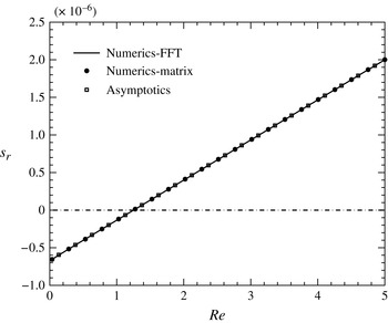
The growth rate,
 $s_{r}$
, versus the Reynolds number,
 $\mathit{Re}$
, for a falling liquid film when
 ${\it\Theta}=0$
,
 ${\it\theta}={\rm\pi}/4$
,
 $k=0.001$
and
 $\mathit{Ka}=1988.5$
.

5.1.1. Case I: no gas flow
To verify our numerical procedure, we first switch off the gas flow and examine whether we recover the linear stability results for a falling film (see, e.g. Yih Reference Yih1963). This is realised by setting
 $\hat{{\it\tau}}_{w0}=0$
,
 ${\it\tau}_{w1}(k/{\it\nu})=0$
and
 $P_{w1}(k/{\it\nu})=0$
. The asymptotic solution for small
 $k$
is given by
 $$\begin{eqnarray}\displaystyle {\it\phi} & = & \displaystyle (z+1)^{2}+k\Big[{\textstyle \frac{1}{240}}\text{i}\mathit{Re}z^{5}-{\textstyle \frac{1}{48}}\text{i}\mathit{Re}z^{4}+{\textstyle \frac{1}{6}}\left(-{\textstyle \frac{3}{4}}\text{i}\mathit{Re}+\text{i}\cot {\it\theta}\right)z^{3}\nonumber\\ \displaystyle & & \displaystyle +\,{\textstyle \frac{1}{2}}\left(-{\textstyle \frac{41}{120}}\text{i}\mathit{Re}+{\textstyle \frac{2}{3}}\text{i}\cot {\it\theta}+2\right)z^{2}+\left(-{\textstyle \frac{17}{240}}\text{i}\mathit{Re}+{\textstyle \frac{1}{6}}\text{i}\cot {\it\theta}+2\right)z+1\Big]+\cdots \,,\qquad\end{eqnarray}$$
 $$\begin{eqnarray}\displaystyle c & = & \displaystyle 2+\text{i}k\left({\textstyle \frac{8}{15}}\mathit{Re}-{\textstyle \frac{2}{3}}\cot {\it\theta}\right)+\cdots \,,\end{eqnarray}$$
 $$\begin{eqnarray}s_{r}=-\text{Re}(\text{i}kc)\equiv k^{2}\left({\textstyle \frac{8}{15}}\mathit{Re}-{\textstyle \frac{2}{3}}\cot {\it\theta}\right).\end{eqnarray}$$
The flat-film solution becomes unstable when
 $s_{r}>0$
, from which one can deduce the classical result that the critical Reynolds number at which the instability sets in is
 $$\begin{eqnarray}\mathit{Re}_{c}={\textstyle \frac{5}{4}}\cot {\it\theta}.\end{eqnarray}$$
Figure 3 shows the growth rate of the disturbance,
 $s_{r}$
, as a function of the Reynolds number,
 $\mathit{Re}$
, with the wavenumber
 $k=0.001$
when
 ${\it\theta}={\rm\pi}/4$
and
 $\mathit{Ka}=1988.5$
. Our computations by two different techniques, namely ‘fast Fourier transform (FFT)-based’ and ‘matrix-based’, agree very well with the asymptotic result. For details on the numerical scheme, the reader is referred to appendix A. Beyond the critical Reynolds number (
 $\mathit{Re}_{c}\equiv 5\cot {\it\theta}/4$
), the flat-film solution becomes unstable and the growth rate increases with increasing
 $\mathit{Re}$
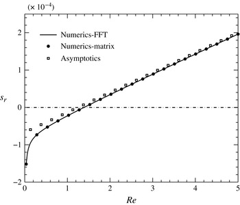
. As we increase the wavenumber (
 $k=0.01$
) further, the growth rate increases for any given
 $\mathit{Re}$
, but the numerics still predicts the critical Reynolds number very well (as shown in figure 4).
The growth rate,
 $s_{r}$
, versus the Reynolds number,
 $\mathit{Re}$
, for a falling liquid film when
 ${\it\Theta}=0$
,
 ${\it\theta}={\rm\pi}/4$
,
 $k=0.01$
and
 $\mathit{Ka}=1988.5$
.

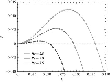
Figure 5 shows the growth rates corresponding to the dominant normal mode for the case of a vertically falling liquid film (
 ${\it\theta}={\rm\pi}/2$
) for various
 $\mathit{Re}$
. As can be observed from the plot, the vertically falling liquid film is unstable to long-wavelength disturbances (for any
 $\mathit{Re}$
), and the band of unstable wavenumbers increases as
 $\mathit{Re}$
is increased. As the wavenumber is increased beyond a particular value, the growth rate becomes negative, implying that the short-wave disturbances are damped.
The growth rate,
 $s_{r}$
, versus the wavenumber,
 $k$
, for a falling liquid film when
 ${\it\Theta}=0$
,
 ${\it\theta}={\rm\pi}/2$
and
 $\mathit{Ka}=1988.5$
. The solid curves correspond to the solutions from the ‘FFT-based’ method and the open circles to the solutions from the ‘matrix-based’ technique.

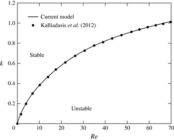
Another way to assess the linear stability of the falling film system is to consider the neutral stability curves. In figure 6, we compare the neutral curves computed from our OS formulation (with the gas flow switched off) with those of Kalliadasis et al. (Reference Kalliadasis, Ruyer-Quil, Scheid and Velarde2012) for the parameter values
 $\mathit{Ka}=528.8$
and
 ${\it\theta}={\rm\pi}/2$
, and we find excellent agreement.
The neutral stability curve for a vertically falling film (
 ${\it\theta}={\rm\pi}/2$
) when
 ${\it\Theta}=0$
and
 $\mathit{Ka}=528.8$
. The solid curve corresponds to our OS system, whereas the closed circles correspond to the results of Kalliadasis et al. (Reference Kalliadasis, Ruyer-Quil, Scheid and Velarde2012).

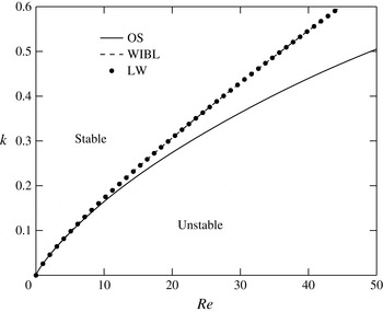
Finally, we compare the neutral curves obtained by solving the dispersion relations of the LW model (4.15) and the WIBL model (4.18) with the OS system for the vertical configuration (
 ${\it\theta}={\rm\pi}/2$
) and
 $\mathit{Ka}=1988.5$
. From figure 7, it can be observed that the LW and WIBL models correctly predict the linear stability threshold for
 $\mathit{Re}$
up to
 $\simeq 10$
, beyond which the agreement becomes poorer as the inertial effects become important, which are not captured by the low-dimensional models. It can also be observed that the results for the WIBL model are in much better agreement with the OS results than those of the LW model.
The neutral stability curve for a vertically falling film (
 ${\it\theta}={\rm\pi}/2$
) when
 ${\it\Theta}=0$
and
 $\mathit{Ka}=1988.5$
. The solid curve corresponds to our OS system, the closed circles correspond to the LW model and the dashed curve corresponds to the WIBL model.

5.1.2. Case II: with gas flow
Following a few reasonable approximations in the gas flow (Lin et al. Reference Lin, Tseluiko and Kalliadasis2014), the asymptotic solution for the falling film in the presence of counter-current gas is given by
 $$\begin{eqnarray}\displaystyle {\it\phi} & = & \displaystyle (z+1)^{2}+k\Big[{\textstyle \frac{1}{480}}\text{i}\mathit{Re}(2+\hat{{\it\tau}}_{w0})z^{5}-{\textstyle \frac{1}{96}}\text{i}\mathit{Re}(2+\hat{{\it\tau}}_{w0})z^{4}-{\textstyle \frac{1}{48}}\text{i}\big(3\mathit{Re}(2+\hat{{\it\tau}}_{w0})\nonumber\\ \displaystyle & & \displaystyle +\,\cot {\it\theta}\big)z^{3}+{\textstyle \frac{1}{480}}(-\text{i}\mathit{Re}(2+\hat{{\it\tau}}_{w0})+160\text{i}\cot {\it\theta}+480)z^{2}\nonumber\\ \displaystyle & & \displaystyle +\,{\textstyle \frac{1}{480}}(-17\text{i}\mathit{Re}(2+\hat{{\it\tau}}_{w0})+80\text{i}\cot {\it\theta}+960)z+1\Big]+\cdots \,,\end{eqnarray}$$
 $$\begin{eqnarray}\displaystyle c & = & \displaystyle 2+\hat{{\it\tau}}_{w0}-2k|\hat{{\it\tau}}_{w0}|+\text{i}k\left({\displaystyle \frac{4\mathit{Re}}{15}}(2+\hat{{\it\tau}}_{w0})-{\displaystyle \frac{2}{3}}\cot {\it\theta}\right)+\cdots \,.\end{eqnarray}$$
 $$\begin{eqnarray}s_{r}=k^{2}\left({\displaystyle \frac{4\mathit{Re}}{15}}(2+\hat{{\it\tau}}_{w0})-{\displaystyle \frac{2}{3}}\cot {\it\theta}\right)\!.\end{eqnarray}$$
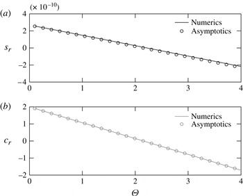
The details of the solution procedure are provided in appendix B. A comparison of the growth rates and phase speeds of the disturbance obtained from asymptotic and numerical approaches is displayed in figure 8, which shows a good agreement. However, the agreement deteriorates when the wavenumber of the disturbance waves is taken to be sufficiently large. Therefore, we resort to numerical treatment of the OS equations and the low-dimensional models.
(a) The growth rate,
 $s_{r}$
, versus the gas parameter,
 ${\it\Theta}$
, and (b) the phase speed,
 $c_{r}$
, versus the gas parameter,
 ${\it\Theta}$
, for a falling liquid film in the presence of counter-current gas when
 ${\it\theta}={\rm\pi}/2$
,
 $k=10^{-5}$
,
 $N=0.4$
and
 $\mathit{Ka}=1988.5$
.

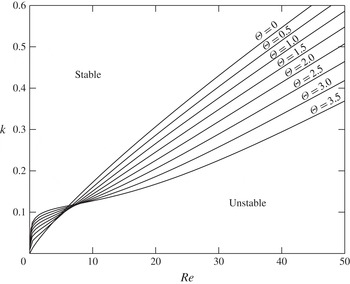
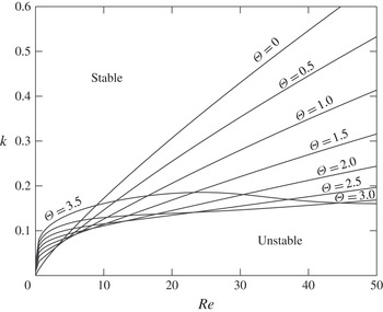
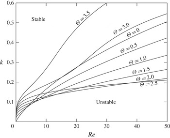
First, we present the neutral curves of the LW model (figure 9), the WIBL model (figure 10) and the OS problem (figure 11). We can observe that the stability boundaries obtained from the LW and WIBL models are slightly different from the OS results, especially for larger values of
 ${\it\Theta}$
. It is also evident that the results for the WIBL model are in better agreement with the OS results than the results for the LW model, at least for
 ${\it\Theta}$
up to the value 2.5. We can observe that for the LW model, the region of stability increases with increasing gas shear for larger values of
 $\mathit{Re}$
. The behaviour is similar for the WIBL model but starts to change for larger values of
 ${\it\Theta}$
. The OS results also show similar behaviour for smaller values of
 ${\it\Theta}$
, but this behaviour drastically changes for larger values of
 ${\it\Theta}$
. This qualitative difference between the results for the reduced model equations and the OS results is attributed to the fact that a consistent derivation of the reduced models (see Tseluiko & Kalliadasis Reference Tseluiko and Kalliadasis2011) is made under assumptions which imply that the normal stress imposed by the turbulent gas is of higher order and is therefore neglected, whereas for the considered helium–methanol system and for sufficiently large values of the gas parameter
 ${\it\Theta}$
, it turns out that the energy production due to the normal stress imposed by the turbulent gas dominates over the energy production due to the tangential stress imposed by the turbulent gas (as is evident from § 5.2).
The neutral stability curves from the LW model for a vertically falling film in contact with counter-current gas flow for various values of the gas shear
 ${\it\Theta}$
, when
 ${\it\theta}={\rm\pi}/2$
,
 $\mathit{Ka}=1988.5$
and
 $N=0.4$
.

The neutral stability curves from the WIBL model for a vertically falling film in contact with counter-current gas flow for various values of the gas shear
 ${\it\Theta}$
, when
 ${\it\theta}={\rm\pi}/2$
,
 $\mathit{Ka}=1988.5$
and
 $N=0.4$
.

The neutral stability curves from the OS equations for a vertically falling film in contact with counter-current gas flow for various values of the gas shear
 ${\it\Theta}$
, when
 ${\it\theta}={\rm\pi}/2$
,
 $\mathit{Ka}=1988.5$
and
 $N=0.4$
.

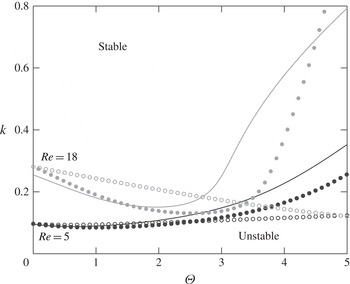
To achieve a better comparison between the various models, we plot the stability boundary in the
 $(k,\,{\rm\Theta})$
-plane for two different values of the Reynolds number,
 $\mathit{Re}=5$
and 18. It can be seen from figure 12 that both the LW and the WIBL model show good agreement with the OS results for
 $\mathit{Re}=5$
, but as the Reynolds number is increased to
 $\mathit{Re}=18$
, the WIBL model overall shows better agreement with the OS results than the LW model.
The neutral stability curves from the different formulations: the solid curves correspond to the OS equation, the open circles to the LW model and the closed circles to the WIBL model, when
 ${\it\theta}={\rm\pi}/2$
,
 $\mathit{Ka}=1988.5$
and
 $N=0.4$
. The black and grey correspond to
 $\mathit{Re}=5$
and
 $\mathit{Re}=18$
, respectively.

5.2. Energy analysis
To investigate the mechanism of instability in the gas–liquid system, we adopt a mechanical energy balance formulation (Smith & Davis Reference Smith and Davis1982; Hooper & Boyd Reference Hooper and Boyd1983; Kelly et al.
Reference Kelly, Goussis, Lin and Hsu1989). The energy balance equation is derived by multiplying the linear equation for the perturbation evolution by
 $(u_{1},v_{1})$
and further by integrating across the interface thickness and over a wavelength
 $(L_{x}=2{\rm\pi}/k_{m})$
, where
 $k_{m}$
is the wavenumber corresponding to the maximum growth rate. The main ideas in the derivation are given below. The linearised equations and the boundary conditions governing the evolution of perturbations are given by
 $$\begin{eqnarray}\displaystyle & \mathit{Re}\left(u_{1t}+u_{0}u_{1x}+v_{1}u_{0y}\right)=-p_{1x}+u_{1xx}+u_{1yy}, & \displaystyle\end{eqnarray}$$
 $$\begin{eqnarray}\displaystyle & \mathit{Re}\left(v_{1t}+u_{0}v_{1x}\right)=-p_{1y}+v_{1xx}+v_{1yy}, & \displaystyle\end{eqnarray}$$
 $$\begin{eqnarray}\displaystyle & u_{1x}+v_{1y}=0, & \displaystyle\end{eqnarray}$$
 $$\begin{eqnarray}\displaystyle & u_{1}=v_{1}=0,\quad \text{at}~y=0, & \displaystyle\end{eqnarray}$$
 $$\begin{eqnarray}\displaystyle & {\it\eta}_{t}+\left(1+\hat{{\it\tau}}_{w0}\right){\it\eta}_{x}=v_{1},\quad \text{at}~y=1, & \displaystyle\end{eqnarray}$$
 $$\begin{eqnarray}\displaystyle & u_{1y}+v_{1x}=[|\hat{{\it\tau}}_{w0}|{\it\nu}{\it\tau}_{w1}(k/{\it\nu})+2]{\it\eta},\quad \text{at}~y=1, & \displaystyle\end{eqnarray}$$
 $$\begin{eqnarray}p_{1}=[|\hat{{\it\tau}}_{w0}|{\it\nu}P_{w1}(k/{\it\nu})+2\cot {\it\theta}]{\it\eta}-\mathit{Re}\mathit{We}{\it\eta}_{xx}-2\hat{{\it\tau}}_{w0}{\it\eta}_{x}-2u_{1x},\quad \text{at}~y=1,\end{eqnarray}$$
where
 ${\it\eta}$
corresponds to the deflection in the free surface about
 $h=1$
. By multiplying (5.8) by
 $u_{1}$
and (5.9) by
 $v_{1}$
, adding the results and integrating over the film thickness and the wavelength (
 $L_{x}$
) we obtain
 $$\begin{eqnarray}\displaystyle & & \displaystyle {\displaystyle \frac{\mathit{Re}}{2L_{x}}}{\displaystyle \frac{\text{d}}{\text{d}t}}\int _{0}^{1}\int _{0}^{L_{x}}\left(u_{1}^{2}+v_{1}^{2}\right)\text{d}x\text{d}y\nonumber\\ \displaystyle & & \displaystyle \quad =-{\displaystyle \frac{\mathit{Re}}{L_{x}}}\int _{0}^{1}\int _{0}^{L_{x}}u_{0y}u_{1}v_{1}\text{d}x\text{d}y-{\displaystyle \frac{1}{L_{x}}}\int _{0}^{1}\int _{0}^{L_{x}}u_{1}p_{1x}\text{d}x\text{d}y-{\displaystyle \frac{1}{L_{x}}}\int _{0}^{1}\int _{0}^{L_{x}}v_{1}p_{1y}\text{d}x\text{d}y\nonumber\\ \displaystyle & & \displaystyle \qquad +\,{\displaystyle \frac{1}{L_{x}}}\int _{0}^{1}\int _{0}^{L_{x}}(u_{1}u_{1xx}+u_{1}u_{1yy}+v_{1}v_{1xx}+v_{1}v_{1yy})\text{d}x\text{d}y.\end{eqnarray}$$
Integration of (5.15) by parts followed by substitution of
 $p_{1}$
from (5.14) results in
 $$\begin{eqnarray}\displaystyle & & \displaystyle {\displaystyle \frac{\mathit{Re}}{2L_{x}}}{\displaystyle \frac{\text{d}}{\text{d}t}}\int _{0}^{1}\int _{0}^{L_{x}}\left(u_{1}^{2}+v_{1}^{2}\right)\text{d}x\text{d}y\nonumber\\ \displaystyle & & \displaystyle \quad =-{\displaystyle \frac{\mathit{Re}}{L_{x}}}\int _{0}^{1}\int _{0}^{L_{x}}u_{0y}u_{1}v_{1}\text{d}x\text{d}y\nonumber\\ \displaystyle & & \displaystyle \qquad -\,{\displaystyle \frac{1}{L_{x}}}\int _{0}^{L_{x}}v_{1}\big[(|\hat{{\it\tau}}_{w0}|{\it\nu}P_{w1}(k/{\it\nu})+2\cot {\it\theta}){\it\eta}-\mathit{Re}\mathit{We}{\it\eta}_{xx}-2\hat{{\it\tau}}_{w0}{\it\eta}_{xx}-2u_{1x}\big]\big|_{y=1}\text{d}x\nonumber\\ \displaystyle & & \displaystyle \qquad +\,{\displaystyle \frac{1}{L_{x}}}\int _{0}^{1}\int _{0}^{L_{x}}\left(u_{1}u_{1xx}+u_{1}u_{1yy}+v_{1}v_{1xx}+v_{1}v_{1yy}\right)\text{d}x\text{d}y.\end{eqnarray}$$
The above equation can be further simplified by substituting the square of the continuity equation (5.10). This yields
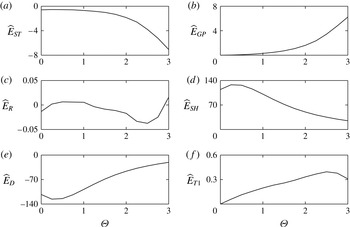
 $$\begin{eqnarray}E_{K}=E_{ST}+E_{GP}+E_{R}+E_{SH}+E_{D}+E_{T1},\end{eqnarray}$$
where
 $$\begin{eqnarray}E_{K}={\displaystyle \frac{1}{2L_{x}}}{\displaystyle \frac{\text{d}}{\text{d}t}}\int _{0}^{1}\int _{0}^{L_{x}}\left(u_{1}^{2}+v_{1}^{2}\right)\text{d}x\text{d}y\end{eqnarray}$$
is the rate of change of ‘kinetic energy’ of the disturbance, which is proportional to the growth rate. The disturbance energy production due to surface tension forces is given by
 $$\begin{eqnarray}E_{ST}={\displaystyle \frac{\mathit{We}}{L_{x}}}\int _{0}^{L_{x}}v_{1}\big|_{1}{\it\eta}_{xx}\text{d}x.\end{eqnarray}$$
The rate of work done by the pressure gradient (due to gas flow and gravity) in deforming the interface is
 $$\begin{eqnarray}E_{GP}=-{\displaystyle \frac{1}{L_{x}\mathit{Re}}}\int _{0}^{L_{x}}v_{1}\big|_{1}[|\hat{{\it\tau}}_{w0}|{\it\nu}P_{w1}(k/{\it\nu})+2\cot {\it\theta}]{\it\eta}\text{d}x,\end{eqnarray}$$
whereas the term
 $E_{R}$
corresponds to the rate of energy transfer from the mean flow of the liquid to the disturbance by means of Reynolds stresses, and is given by
 $$\begin{eqnarray}E_{R}=-{\displaystyle \frac{1}{L_{x}}}\int _{0}^{1}\int _{0}^{L_{x}}u_{0y}u_{1}v_{1}\text{d}x\text{d}y.\end{eqnarray}$$
The work done by the disturbance shear force at the interface is represented by
 $$\begin{eqnarray}E_{SH}={\displaystyle \frac{1}{L_{x}\mathit{Re}}}\int _{0}^{L_{x}}u_{1}\big|_{1}\left[u_{1y}+v_{1x}\right]_{1}\text{d}x,\end{eqnarray}$$
whereas the rate of dissipation of energy by viscous forces is
 $$\begin{eqnarray}E_{D}=-{\displaystyle \frac{1}{L_{x}\mathit{Re}}}\int _{0}^{1}\int _{0}^{L_{x}}[2(u_{1x})^{2}+\left(u_{1y}+v_{1x}\right)^{2}+2\left(v_{1y}\right)^{2}]\text{d}x\text{d}y.\end{eqnarray}$$
Finally, the work done by the applied shear stress at the interface due to counter-current gas flow is given by
 $$\begin{eqnarray}E_{T1}={\displaystyle \frac{2\hat{{\it\tau}}_{w0}}{L_{x}\mathit{Re}}}\int _{0}^{L_{x}}v_{1}\big|_{1}{\it\eta}_{x}\text{d}x.\end{eqnarray}$$
The various energy quantities (5.18)–(5.24) in the kinetic energy equation (5.17) can be evaluated by making use of the solution obtained by solving the eigenvalue problem (A 7). The variables involved in the energy terms are derived once the eigenvalue
 $c$
and the eigenfunction
 ${\it\phi}$
are obtained by solving the OS problem. In order to perform the integration along the cross-streamwise direction, we employ a pseudo-spectral approach, whereas integration along the streamwise direction is carried out using the trapezoidal rule.
In this energy analysis, we are interested in the energy composition for the most dominant normal mode; therefore we consider wavenumbers corresponding to the maximum growth rate. The various energy terms in the kinetic energy equation are evaluated for increasing values of the gas flow rate
 ${\it\Theta}$
using the numerical methodology described above, and the results, scaled with the kinetic energy
 $E_{K}$
, are shown in figure 13. For the case of a vertically falling film in the absence of gas flow (
 ${\it\Theta}=0$
), the main contribution to energy production comes from the disturbance shear force at the interface
 $\widehat{E}_{SH}$
, whereas some of this energy is dissipated by the viscous forces
 $\widehat{E}_{D}$
. As the gas flow is switched on, the energy production has a contribution from the applied shear stress
 $\widehat{E}_{T1}$
in addition to the applied pressure gradient due to gas flow and gravity
 $\widehat{E}_{GP}$
. (We note that for the vertical configuration of the channel considered here, the contribution due to gravity in
 $\widehat{E}_{GP}$
vanishes.) It can be observed that
 $\widehat{E}_{T1}$
dominates over
 $\widehat{E}_{GP}$
for smaller values of the gas flow rate, whereas
 $\widehat{E}_{GP}$
is dominant for larger gas flow rates. The contribution from the Reynolds stresses
 $\widehat{E}_{R}$
is negligible for the moderate values of the Reynolds number considered in this study.
Plots of various energy terms in (5.17) normalised with the total kinetic energy
 $E_{K}$
as a function of the gas shear
 ${\it\Theta}$
, when
 $\mathit{Re}_{0}=10$
,
 ${\it\theta}={\rm\pi}/2$
,
 $\mathit{Ka}=1988.5$
and
 $N=0.4$
.

5.3. Absolute and convective instabilities
In this section, we outline our methodology to analyse absolute and convective instabilities by considering the dispersion relation obtained from the LW model. Our analysis follows that by Fokas & Papageorgiou (Reference Fokas and Papageorgiou2005). We note first that the dispersion relation
 $s(k)$
is not analytic at zero and, therefore, it is not possible to study absolute and convective instabilities in a straightforward way by analysing the saddle point of the real part of the dispersion relation and applying the Briggs pinching criterion, see e.g. Huerre & Monkewitz (Reference Huerre and Monkewitz1990). To begin, let us assume that
 $f(x,\,0)=f_{0}(x)$
is the given initial condition. Therefore, the solution of the linearised equation can be written as
 $$\begin{eqnarray}f(x,\,t)=\frac{1}{2{\rm\pi}}\int _{-\infty }^{\infty }\text{e}^{s(k)t+\text{i}kx}\hat{f}_{0}(k)\hspace{2.22198pt}\text{d}k,\end{eqnarray}$$
where
 $\hat{f}_{0}(k)$
is the Fourier transform of the initial condition:
 $$\begin{eqnarray}\hat{f}_{0}(k)=\int _{-\infty }^{\infty }\text{e}^{-\text{i}kx}f_{0}(x)\hspace{2.22198pt}\text{d}x.\end{eqnarray}$$
There are two possibilities. If
 $\text{Re}[s(k)]\leqslant 0$
for all
 $k$
, the flat-film solution is linearly stable. On the other hand, if
 $\text{Re}[s(k)]>0$
at least for some
 $k$
, then the flat-film solution is unstable, and the instability could be either absolute or convective. Noting that
 ${\it\tau}_{w1}(-{\it\alpha})=\overline{{\it\tau}_{w1}({\it\alpha})}$
for real
 ${\it\alpha}$
, where the bar denotes complex conjugation (see Vellingiri et al.
Reference Vellingiri, Tseluiko, Savva and Kalliadasis2013), the growth rate can be written as
 $$\begin{eqnarray}s(k)=\left\{\begin{array}{@{}ll@{}}-\text{i}ak+bk^{2}-ck^{4}-\text{i}\text{d}k\hspace{2.22198pt}\overline{{\it\tau}_{w1}(k/{\it\nu})}\equiv s_{-}(k)\quad & \text{if}~k<0,\\ -\text{i}ak+bk^{2}-ck^{4}-\text{i}\text{d}k\hspace{2.22198pt}{\it\tau}_{w1}(k/{\it\nu})\equiv s_{+}(k)\quad & \text{if}~k\geqslant 0.\end{array}\right.\end{eqnarray}$$
The growth rates are related by
 $s_{-}(-k)=\overline{s_{+}(k)}$
. We denote the real part of the growth rate as
 $s_{r}(k)\equiv \text{Re}[s_{+}(k)]=bk^{2}-ck^{4}+\text{d}k\hspace{2.22198pt}\text{Im}[{\it\tau}_{w1}(k/{\it\nu})]$
. The integral (5.25) can be rewritten as
 $$\begin{eqnarray}f(x,\,t)=\frac{1}{2{\rm\pi}}[I(x,\,t)+J(x,\,t)],\end{eqnarray}$$
where
 $$\begin{eqnarray}I(x,\,t)=\left(\int _{-\infty }^{-k_{1}}+\int _{k_{1}}^{\infty }\right)\text{e}^{s(k)t+\text{i}kx}\hat{f}_{0}(k)\hspace{2.22198pt}\text{d}k\end{eqnarray}$$
and
 $$\begin{eqnarray}J(x,\,t)=\left(\int _{-k_{1}}^{0}+\int _{0}^{k_{1}}\right)\text{e}^{s(k)t+\text{i}kx}\hat{f}_{0}(k)\hspace{2.22198pt}\text{d}k,\end{eqnarray}$$
with
 $k_{1}$
being the critical wavenumber below which the flat-film solution is unstable. For fixed
 $x/t$
,
 $I(x,\,t)$
goes to zero as
 $t$
increases. Therefore, it is sufficient to analyse the other integral,
 $J(x,\,t)$
:
 $$\begin{eqnarray}\displaystyle J(x,\,t) & = & \displaystyle \int _{-k_{1}}^{0}\text{e}^{s_{-}(k)t+\text{i}kx}\hat{f}_{0}(k)\hspace{2.22198pt}\text{d}k+\int _{0}^{k_{1}}\text{e}^{s_{+}(k)t+\text{i}kx}\hat{f}_{0}(k)\hspace{2.22198pt}\text{d}k\end{eqnarray}$$
 $$\begin{eqnarray}\displaystyle & = & \displaystyle \int _{0}^{k_{1}}\text{e}^{s_{-}(-k)t-\text{i}kx}\hat{f}_{0}(-k)\hspace{2.22198pt}\text{d}k+\int _{0}^{k_{1}}\text{e}^{s_{+}(k)t+\text{i}kx}\hat{f}_{0}(k)\hspace{2.22198pt}\text{d}k.\end{eqnarray}$$
By making use of the fact that
 $s_{-}(-k)=\overline{s_{+}(k)}$
for real
 $k$
, and that
 $\hat{f}_{0}(-k)=\overline{\hat{f}_{0}(k)}$
as
 $f_{0}(x)$
is a real function, we obtain
 $$\begin{eqnarray}\displaystyle J(x,\,t) & = & \displaystyle \int _{0}^{k_{1}}\left[\text{e}^{\overline{s_{+}(k)}t-\text{i}kx}\overline{\hat{f}_{0}(k)}+\text{e}^{s_{+}(k)t+\text{i}kx}\hat{f}_{0}(k)\right]\hspace{2.22198pt}\text{d}k\end{eqnarray}$$
 $$\begin{eqnarray}\displaystyle & = & \displaystyle \int _{0}^{k_{1}}\left[\,\overline{\text{e}^{s_{+}(k)t+\text{i}kx}\hat{f}_{0}(k)}+\text{e}^{s_{+}(k)t+\text{i}kx}\hat{f}_{0}(k)\right]\hspace{2.22198pt}\text{d}k\end{eqnarray}$$
 $$\begin{eqnarray}\displaystyle & = & \displaystyle 2\text{Re}\left[K(x,\,t)\right],\end{eqnarray}$$
where
 $$\begin{eqnarray}K(x,\,t)=\int _{0}^{k_{1}}\text{e}^{s_{+}(k)t+\text{i}kx}\hat{f}_{0}(k)\hspace{2.22198pt}\text{d}k.\end{eqnarray}$$
The function
 $s_{+}(k)$
is defined for real non-negative values of
 $k$
, since
 ${\it\tau}_{w1}({\it\alpha})$
is obtained by solving equation (3.34) in Tseluiko & Kalliadasis (Reference Tseluiko and Kalliadasis2011) with homogeneous boundary conditions (3.37) and (3.38) in the same study for positive values of
 ${\it\alpha}$
. Noticing that the coefficients in (3.34) in Tseluiko & Kalliadasis (Reference Tseluiko and Kalliadasis2011) are analytic functions of
 ${\it\alpha}$
, we can obtain an analytic continuation of
 ${\it\tau}_{w1}({\it\alpha})$
from the non-negative real semi-axis to the whole complex plane by solving equation (3.34) in Tseluiko & Kalliadasis (Reference Tseluiko and Kalliadasis2011) with homogeneous boundary conditions (3.37) and (3.38) in the same study when
 ${\it\alpha}$
is an arbitrary complex number. Then the analysis of
 $K(x,\,t)$
depends on the topology of the curves
 $s_{r}(k)=0$
in the complex
 $k$
-plane, where
 $s_{r}(k)$
denotes the real part of
 $s_{+}(k)$
. There are two possibilities.
Case I: there is part of the curve
 $s_{r}(k)=0$
that connects the origin
 $(0,0)$
and
 $(k_{1},0)$
in the
 $(k_{r},k_{i})$
-plane, with
 $k_{r}$
and
 $k_{i}$
denoting the real and imaginary parts of
 $k$
respectively. In addition, if
 $\hat{f}_{0}(k)$
can be analytically continued off the real axis so that
 $\hat{f}_{0}(k)$
is analytic in a neighbourhood of the curve
 $s_{r}(k)=0$
connecting the points
 $(0,0)$
and
 $(k_{1},0)$
(this is the case, for example, when
 $f_{0}(x)$
has a sufficiently fast exponential decay as
 $|x|\rightarrow \infty$
), the integration contour for
 $K(x,t)$
can be deformed to follow that part of the curve
 $s_{r}(k)=0$
that connects
 $(0,0)$
to
 $(k_{1},0)$
. The Riemann–Lebesgue lemma then implies that for a fixed
 $x$
,
 $K(x,t)\rightarrow 0$
as
 $t\rightarrow \infty$
, and we have convective instability.
Case II: the other possibility is that it is impossible to connect the origin with
 $(k_{1},\,0)$
using part of the curve
 $s_{r}(k)=0$
in the
 $(k_{r},k_{i})$
-plane. In such a scenario, there must exist a saddle point (also called the pinch point) of
 $s_{r}(k)$
, at which
 $s_{r}(k)$
is positive, so that the integration contour can be deformed into a steepest descent path passing through this saddle point. Here,
 $K(x,\,t)$
is seen to grow for a fixed
 $x$
as
 $t\rightarrow \infty$
(Hinch Reference Hinch1991), and the type of instability in this case is absolute. We also note here that the saddle point corresponds to the mode with zero group velocity.
The details of the numerical scheme to compute the curves
 $s_{r}(k)=0$
in the
 $(k_{r},k_{i})$
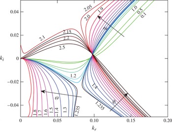
-plane for the OS problem are provided in appendix C. We begin by presenting in figure 14 the curves
 $s_{r}(k)=0$
in the
 $(k_{r},k_{i})$
-plane for various values of the gas shear,
 ${\it\Theta}$
, for
 $\mathit{Re}=5$
, corresponding to the dispersion relation (4.15) obtained from the LW model. It can be observed from figure 14 that for sufficiently small values of
 ${\it\Theta}$
, the origin is connected to
 $(k_{r},0)$
. Therefore, we have convective instability. This is to be expected, as any localised disturbance introduced to the system is convected downstream, in the positive
 $x$
direction. The situation is similar for large values of
 ${\it\Theta}$
, but the disturbance is convected in the negative
 $x$
direction. However, there exists a band of gas flow rates (
 $1.235\leqslant {\it\Theta}\leqslant 2.1$
) for which the origin is not connected to
 $(k_{r},0)$
by
 $s_{r}(k)=0$
, and the instability is absolute.
The curves of
 $s_{r}(k)=0$
in the complex wavenumber plane
 $(k_{r},k_{i})$
from the LW model for various values of the gas shear,
 ${\it\Theta}$
, when
 $\mathit{Re}_{0}=10$
,
 ${\it\theta}={\rm\pi}/2$
,
 $\mathit{Ka}=1988.5$
and
 $N=0.4$
.

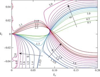
Figure 15 shows the curves
 $s_{r}(k)=0$
corresponding to the quadratic dispersion relation (4.18) obtained from the WIBL model. We note that for the WIBL model there exist two branches,
 $s_{r1}(k)$
and
 $s_{r2}(k)$
. However, for the parameter space under consideration, only for one of these branches does there exist a band of unstable wavenumbers. We denote this branch by
 $s_{r}(k)$
. The results obtained using the WIBL model are similar to those obtained from the LW model with only minor differences.
The curves of
 $s_{r}(k)=0$
in the complex wavenumber plane
 $(k_{r},k_{i})$
from the WIBL model for various values of the gas shear,
 ${\it\Theta}$
, when
 $\mathit{Re}_{0}=10$
,
 ${\it\theta}={\rm\pi}/2$
,
 $\mathit{Ka}=1988.5$
and
 $N=0.4$
.

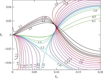
Finally, we present the curves
 $s_{r}(k)=0$
in the
 $(k_{r},k_{i})$
-plane corresponding to the dominant mode in the OS problem (figure 16), which also turns out to be the only unstable mode for the parameter values considered. The results are again similar to those presented earlier for the LW and WIBL models, with the region of absolute instability predicted to be
 $1.21\leqslant {\it\Theta}\leqslant 2.1$
. This is not very surprising as the liquid flow rate that we have considered is sufficiently small for the low-dimensional models to have good agreement with the OS results (see also figure 12, from the temporal analysis). Moreover, we find that the WIBL model has a better quantitative agreement with the OS equations than the LW model in the flow regime considered.
The curves of
 $s_{r}(k)=0$
in the complex wavenumber plane
 $(k_{r},k_{i})$
by solving the OS problem for various values of the gas shear,
 ${\it\Theta}$
, when
 $\mathit{Re}_{0}=10$
,
 ${\it\theta}={\rm\pi}/2$
,
 $\mathit{Ka}=1988.5$
and
 $N=0.4$
.

We note, in addition, that the nonlinear computations of the WIBL model of Tseluiko & Kalliadasis (Reference Tseluiko and Kalliadasis2011) reveal that the flooding point (defined as the point at which there appear large-amplitude nearly stationary waves) is close to
 ${\it\Theta}\sim 2.5$
. Interestingly, this flooding point is also close to the upper limit of the absolute instability regime (
 ${\it\Theta}\sim 2.1$
) predicted by our analysis.
5.3.1. Influence of the inclination angle
We analyse the influence of the inclination angle on the onset of absolute and convective instabilities by performing the analysis for the OS problem for various values of the inclination angle
 ${\it\theta}$
, namely
 ${\rm\pi}/3$
,
 ${\rm\pi}/4$
and
 ${\rm\pi}/6$
, with the modified Reynolds number being fixed at
 $\mathit{Re}_{0}=10$
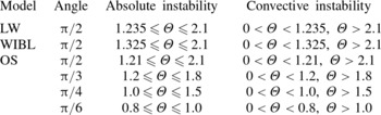
. Table 1 shows the regimes of absolute and convective instabilities for the various angles (the results for
 ${\rm\pi}/2$
are shown for the various models, whereas for the other angles the results are obtained by performing the analysis for the OS problem only). It should be noted that as the inclination angle of the channel is decreased, the liquid flow rate decreases as well and the stabilisation of the interface is enhanced by the normal component of gravity resulting from the decrease of the inclination angle. It can be observed that the increase in the inclination angle results in a delay of the onset of absolute instability.
Absolute and convective instability regimes computed using various models when
 $\mathit{Re}_{0}=10$
,
 $\mathit{Ka}=1988.5$
and
 $N=0.4$
.

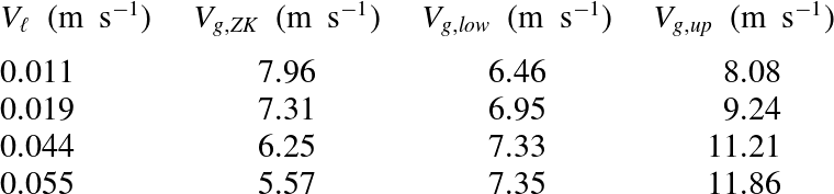
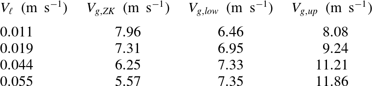
Comparison with experiments of Zapke & Kröger (Reference Zapke and Kröger2000a
) with air and methanol as working fluids (see their figure 8). Here,
 $V_{\ell }$
denotes the average liquid velocity,
 $V_{g,ZK}$
corresponds to the average flooding gas velocity in Zapke & Kröger (Reference Zapke and Kröger2000a
) and
 $V_{g,low}$
and
 $V_{g,up}$
correspond to the lower and upper limits of absolute instability respectively, computed using our analysis.
5.3.2. Comparison with experiments
In order to verify the predictions of our model, we consider air and methanol as working fluids in a vertical channel; these fluids were also considered in the experiments by Zapke & Kröger (Reference Zapke and Kröger2000a ) (see their figure 8). As the parameters fall in the regime where our WIBL model was shown to have a good agreement with the OS problem, we consider the WIBL model to compute the limits of absolute instability, which we believe has a close connection to flooding. The comparison shown in table 2 indicates a fair agreement. The experimental flooding point turns out to be close to the region of absolute instability (moreover, it turns out that the flooding point lies between the absolute instability boundaries, except for the last line in the table), but it has to be noted that the trend is slightly different, i.e. the gas velocities for the absolute instability boundaries monotonically increase as the liquid velocity increases, whereas in the experiments of Zapke & Kröger (Reference Zapke and Kröger2000a ) the flooding gas velocity is found to decrease with the liquid velocity (which appears to be counterintuitive). However, confidence limit error bars were not provided for the experiments of Zapke & Kröger (Reference Zapke and Kröger2000a ), and, therefore, it is not really clear how accurate the experimental findings are. Another explanation for the differences between our theoretical predictions and the experiments may be that our analysis assumes two-dimensional flow, whereas two-dimensionality may not be valid in the experiments. Moreover, the observed differences may be related to the way in which Zapke & Kröger (Reference Zapke and Kröger2000a ) define flooding and their interpretation of flooding, namely they state that flooding occurs when a vortex (large-amplitude wave) formed at the inlet of the channel has grown to such an extent that it obstructs the flow of the gas (i.e. the height of the wave is comparable with the height of the channel), resulting in the liquid travelling up past the injection point. (We note that Zapke & Kröger (Reference Zapke and Kröger2000a ) used a channel with a rectangular cross-section of width 10 mm and height 50 mm.) However, the width of the channel considered in our model is assumed to be very large compared with the liquid film thickness, so that the amplitude of the standing wave formed at the point of wave reversal is not comparable with the channel width. Notwithstanding the above mentioned disparities, our linear theory appears to be useful in predicting the nonlinear phenomenon of flooding, but clearly further detailed experiments are needed to test our theoretical predictions carefully.
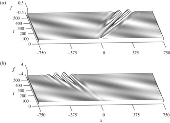
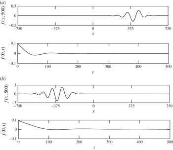
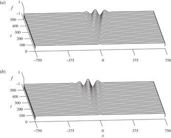
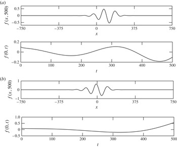
Time-dependent computation of the linearised WIBL model subject to a localised disturbance, showing convective instability for (a)
 ${\it\Theta}=1.0$
and (b)
 ${\it\Theta}=2.2$
, with
 $\mathit{Re}_{0}=10$
,
 ${\it\theta}={\rm\pi}/2$
,
 $\mathit{Ka}=1988.5$
and
 $N=0.4$
. The three-dimensional plot is inclined here for better visualisation.

5.4. Time-dependent computations
We further explore the absolute and convective instability regimes predicted by our linear analysis in § 5.3, by solving the linearised WIBL model (4.16) and (4.17) as an initial-value problem subject to a localised initial condition. This is carried out numerically using a scheme that is based on a Fourier pseudo-spectral representation of the derivatives along the spatial direction and an adaptive stepping along time, e.g. Tseluiko et al. (Reference Tseluiko, Saprykin, Duprat, Giorgiutti-Dauphiné and Kalliadasis2010). We choose the initial condition of the interface disturbance,
 $f(x,t)$
, to be localised about
 $x=0$
, namely, we choose the Gaussian function
 $f(x,0)=0.1\exp (-0.5x^{2})$
. In addition, we choose
 $g(x,0)=0$
. The liquid Reynolds number is taken to be
 $\mathit{Re}=5$
, consistent with that in the previous section. The equations are integrated on a long periodic domain,
 $[-750,750]$
, for a sufficiently long time, say
 $t\approx 500$
, to determine the evolution of the wavepackets.
We begin with a relatively small value of the gas shear,
 ${\it\Theta}=1.0$
, and the corresponding evolution of the disturbance is depicted as a space–time plot in figure 17(a). It can be observed that the wavepacket starts propagating downstream along the positive
 $x$
direction, therefore the instability is convective. On the other side of the gas flow spectrum, e.g. for
 ${\it\Theta}=2.2$
, the instability is again convective, with the wavepacket propagating upstream along the negative
 $x$
direction (figure 17
b). This can be further confirmed by examining the wave profile at a sufficiently long time instant and the time evolution of the disturbance,
 $f(x,t)$
, at
 $x=0$
, see the top and bottom panels of figure 18 respectively. From figure 18, it can be ascertained that the wave profiles for
 ${\it\Theta}=1.0$
and
 ${\it\Theta}=2.2$
are convected in the positive and negative
 $x$
directions (see the top panels), and also the disturbance,
 $f(0,t)$
eventually decays to zero (see the bottom panels). This is consistent with the analytical results discussed above. For intermediate values of the gas flow rate, e.g. for
 ${\it\Theta}=1.5$
and
 ${\it\Theta}=1.65$
shown in figure 19, the wavepackets invade both the negative and the positive
 $x$
directions, and for longer times they are expected to contaminate the whole domain. This can also be established from figure 20, from which it can be concluded that the disturbance
 $f(0,t)$
does not decay to zero. These results agree with the band of absolutely unstable gas flow rates,
 $1.2\leqslant {\it\Theta}\leqslant 2.1$
, predicted by our analysis of various models in § 5.3.
Time-dependent computations of the linearised WIBL model depicting wave profiles at
 $t=500$
and the time evolution of the disturbance at
 $x=0$
for (a)
 ${\it\Theta}=1.0$
and (b)
 ${\it\Theta}=2.2$
, with
 $\mathit{Re}_{0}=10$
,
 ${\it\theta}={\rm\pi}/2$
,
 $\mathit{Ka}=1988.5$
and
 $N=0.4$
.

Time-dependent computation of the linearised WIBL model subject to a localised disturbance, showing convective instability for (a)
 ${\it\Theta}=1.5$
and (b)
 ${\it\Theta}=1.65$
, with
 $\mathit{Re}_{0}=10$
,
 ${\it\theta}={\rm\pi}/2$
,
 $\mathit{Ka}=1988.5$
and
 $N=0.4$
. The three-dimensional plot is inclined here for better visualisation.

Time-dependent computations of the linearised WIBL model depicting wave profiles at
 $t=500$
and the time evolution of the disturbance at
 $x=0$
for (a)
 ${\it\Theta}=1.5$
and (b)
 ${\it\Theta}=1.65$
, with
 $\mathit{Re}_{0}=10$
,
 ${\it\theta}={\rm\pi}/2$
,
 $\mathit{Ka}=1988.5$
and
 $N=0.4$
.

6. Concluding remarks
We have analysed the linear stability of a gas–liquid system in an inclined channel, where a thin liquid film flowing along the bottom wall is in contact with a counter-current gas flow occupying the rest of the channel. The liquid film is considered to be laminar whereas the counter-current gas flow is turbulent. The influence of gas flow enters the liquid problem through the boundary conditions at the gas–liquid interface, as expected. This challenging gas–liquid problem can be decoupled and solved independently by making a number of reasonable assumptions (Tseluiko & Kalliadasis Reference Tseluiko and Kalliadasis2011).
We considered two non-local reduced-order model equations for the interface thickness (measured from the liquid layer), namely the LW and WIBL models derived by Tseluiko & Kalliadasis (Reference Tseluiko and Kalliadasis2011), and also formulated the OS system of equations from the full governing equations and boundary conditions. A significant advantage with the OS equations from a stability perspective is that they are applicable for all values of the liquid Reynolds number and wavenumber. Moreover, the comparison of the results for the reduced model equations with the OS results is important for finding out the ranges of validity of the reduced models. In addition to performing the temporal stability analysis, we carried out an energy analysis using the linearised version of the full Navier–Stokes equation to understand the physical nature of the instability. We have also developed a generalised methodology based on Fokas & Papageorgiou (Reference Fokas and Papageorgiou2005) for the non-local equations with non-analytic dispersion relations to scrutinise absolute and convective instabilities. This approach involves analysing the nature of growth-rate curves in the complex wavenumber plane. If the origin is connected to the purely real wavenumber root in the complex wavenumber plane by the vanishing growth-rate curve, then the instability is convective. On the other hand, if it is impossible to connect the origin to the real root by the zero-growth-rate curve, and there exists a saddle point (which is also the pinch point) where the growth rate is positive, we have absolute instability. This saddle point also corresponds to the normal mode whose group velocity is zero.
By applying this methodology to the OS equations, and the low-dimensional models, we obtained the flow conditions for which the system exhibits absolute and convective instabilities. More precisely, we found that for a fixed liquid flow rate, the system is convectively unstable at low and high gas flow rates, where the localised disturbance gets convected in the downstream and upstream directions respectively. However, for a range of intermediate gas flow rates with the liquid flow rate fixed at the same value as before, we have absolute instability, where the disturbance contaminates the whole domain. We have also analysed the effect of the inclination angle on the onset of absolute instability, and we found that larger gas flow rates are required to trigger absolute instability for larger values of the angle of inclination. In general, the results for the WIBL model are found to be in better agreement with the results for the OS equations than the results for the LW model, as the WIBL model is expected to be able to describe the flow behaviour for up to moderate values of the Reynolds number. Further, we supplemented our analysis by performing time-dependent computations of the linearised WIBL model subject to a localised initial condition, which showed good agreement with the predictions of the linear stability analysis. It is interesting to note that the upper limit of the absolute instability regime is close to the flooding point obtained from the fully nonlinear computations of the WIBL model of Tseluiko & Kalliadasis (Reference Tseluiko and Kalliadasis2011). In addition, a comparison of our model predictions with the flooding experiments of Zapke & Kröger (Reference Zapke and Kröger2000a ) shows a fairly good agreement. We can therefore conclude that the linear analysis presented here can be useful in predicting the flooding point.
Acknowledgements
We acknowledge financial support from EPSRC grant No. EP/K504130/1 and ERC Advanced grant No. 247031. The work of D.T. was partly supported by EPSRC Grant No. EP/J001740/1.
Appendix A. Numerical method for the OS problem
The OS equation (4.8) along with the boundary conditions (4.9)–(4.12) is solved using a Chebyshev pseudo-spectral method (Trefethen Reference Trefethen2000; Yatsyshin, Savva & Kalliadasis Reference Yatsyshin, Savva and Kalliadasis2012). By making use of the transformation
 $z=2y-1$
, we map the physical film domain
 $0\leqslant y\leqslant 1$
onto the canonical interval
 $-1\leqslant z\leqslant 1$
. Under this mapping, the OS equation together with the boundary conditions becomes
 $$\begin{eqnarray}\displaystyle & & \displaystyle 16{\it\phi}^{\prime \prime \prime \prime }-8k^{2}{\it\phi}^{\prime \prime }+k^{4}{\it\phi}-\text{i}k\mathit{Re}\left[\left(\frac{z+1}{4}\right)\left(3+2\hat{{\it\tau}}_{w0}-z\right)\left(4{\it\phi}^{\prime \prime }-k^{2}{\it\phi}\right)+2{\it\phi}\right]\nonumber\\ \displaystyle & & \displaystyle \quad =-\text{i}kc\mathit{Re}\left(4{\it\phi}^{\prime \prime }-k^{2}{\it\phi}\right),\end{eqnarray}$$
 $$\begin{eqnarray}{\it\phi}(-1)=0,\quad {\it\phi}^{\prime }(-1)=0,\end{eqnarray}$$
 $$\begin{eqnarray}\displaystyle & {\it\phi}(1)+(1+\hat{{\it\tau}}_{w0})A_{1}=cA_{1}, & \displaystyle\end{eqnarray}$$
 $$\begin{eqnarray}\displaystyle & 4{\it\phi}^{\prime \prime }(1)+k^{2}{\it\phi}(1)-[|\hat{{\it\tau}}_{w0}|{\it\nu}{\it\tau}_{w1}(k/{\it\nu})+2]A_{1}=0, & \displaystyle\end{eqnarray}$$
 $$\begin{eqnarray}\displaystyle & 8{\it\phi}^{\prime \prime \prime }(1)-k[2\text{i}\cot {\it\theta}+\text{i}k^{2}\mathit{We}\mathit{Re}+2k\hat{{\it\tau}}_{w0}+\text{i}|\hat{{\it\tau}}_{w0}|{\it\nu}P_{w1}(k/{\it\nu})]A_{1} & \displaystyle \nonumber\\ \displaystyle & \quad -\,2k[\text{i}\mathit{Re}(1+\hat{{\it\tau}}_{w0})+3k]{\it\phi}^{\prime }(1)+\text{i}k\mathit{Re}\hat{{\it\tau}}_{w0}{\it\phi}(1)=-2\text{i}kc\mathit{Re}{\it\phi}^{\prime }(1), & \displaystyle\end{eqnarray}$$
 $z$
. We could further eliminate
 $A_{1}$
from the system of equations using (A 4), followed by making the substitution for
 $A_{1}$
in (A 3) and (A 5). One could then avoid appending the differentiation matrices with zeros and ones in order to solve for
 $A_{1}$
. Nevertheless, we have made all our computations by retaining
 $A_{1}$
in our model system as a general practice. However, the results obtained by both of these approaches are exactly the same.
Boomkamp et al. (Reference Boomkamp, Boersma, Miesen and Beijnon1997) developed a collocation method based on Chebyshev polynomials to solve the eigenvalue problem governing the stability of parallel two-phase flow, which is similar to the methodology developed by Orszag (Reference Orszag1971) to investigate the stability of Poiseuille’s flow. In our approach, we begin by expanding the eigenfunction
 ${\it\phi}(z)$
as a truncated series of Chebyshev polynomials,
 $T_{i}(z)$
(defined on the interval
 $[-1,1]$
),
 $$\begin{eqnarray}{\it\phi}(z)=\mathop{\sum }_{i=0}^{M}a_{i+1}T_{i}(z),\end{eqnarray}$$
with
 ${\it\phi}$
given on the Chebyshev points,
 $z_{j}=\cos ({\it\beta}_{j})$
,
 ${\it\beta}_{j}=(\,j-1){\rm\pi}/M$
,
 $j=1,\dots ,M+1$
. In the ‘FFT-based’ formulation, Chebyshev differentiation is implemented by using the fast Fourier transform (Trefethen Reference Trefethen2000). The boundary conditions are imposed by replacing the last four rows (corresponding to the highest modes) with five boundary conditions that we have. This results in a generalised matrix eigenvalue problem of the form
 $$\begin{eqnarray}\unicode[STIX]{x1D63C}\boldsymbol{w}=c\unicode[STIX]{x1D63D}\boldsymbol{w},\end{eqnarray}$$
where
 $\boldsymbol{w}=(a_{0},\dots ,a_{M},A_{1})^{\text{T}}$
, and
 $\unicode[STIX]{x1D63C}$
and
 $\unicode[STIX]{x1D63D}$
are square matrices of size
 $M+2$
.
In the ‘matrix-based’ approach, as the name suggests, the derivative of a function is computed by matrix–vector multiplication. The entries of the differentiation matrix are computed by taking the analytical derivative of the interpolating polynomial, followed by evaluation at the Chebyshev points. To enforce the no-slip and no-penetration boundary conditions at the bottom wall, we follow the approach by Trefethen of multiplying the interpolating polynomial by another polynomial (Trefethen Reference Trefethen2000), such that both conditions are satisfied implicitly. This approach enables us to impose the bottom-wall boundary conditions accurately, i.e. exactly at the boundary point. This results in a generalised matrix eigenvalue problem as before, but the square matrices
 $\unicode[STIX]{x1D63C}$
and
 $\unicode[STIX]{x1D63D}$
now are of size
 $M+1$
.
The generalised eigenvalue problem (A 7) is solved using Matlab. The large entries in
 $\unicode[STIX]{x1D63C}$
coming from the higher-order derivatives and the zero rows in
 $\unicode[STIX]{x1D63D}$
(coming from the bottom-wall boundary conditions) result in spurious and ‘infinite’ eigenvalues. We ignore such eigenvalues, and consider only the meaningful finite ones for our calculations. Typically 20–30 collocation points are sufficient to accurately capture the behaviour of the system.
Appendix B. Asymptotic solution for the OS problem in the presence of counter-current gas flow
As in the falling film setting, we perform regular perturbation expansions for the eigenfunction (
 ${\it\phi}$
) and the complex wave velocity (
 $c$
) for the liquid problem, under the assumption of long waves (
 $k\rightarrow 0$
). However, this requires a solution for the gas problem in the LW regime. The idea is to make use of the solution obtained by Lin et al. (Reference Lin, Tseluiko and Kalliadasis2014) for the gas phase, and proceed with the asymptotics for the liquid problem. By substituting the following LW expansions:
 $$\begin{eqnarray}\displaystyle & {\it\phi}={\it\phi}_{0}+\text{i}k{\it\phi}_{1}+\cdots \,, & \displaystyle\end{eqnarray}$$
 $$\begin{eqnarray}\displaystyle & c=c_{0}+\text{i}k{\it\phi}_{1}+\cdots \,, & \displaystyle\end{eqnarray}$$
 $$\begin{eqnarray}\displaystyle & {\it\phi}_{0}^{\prime \prime \prime \prime }=0, & \displaystyle\end{eqnarray}$$
 $$\begin{eqnarray}\displaystyle & (2c_{0}-1-\hat{{\it\tau}}_{w0}){\it\phi}_{0}^{\prime \prime }(1)-{\it\phi}_{0}(1)=0, & \displaystyle\end{eqnarray}$$
 $$\begin{eqnarray}{\it\phi}_{0}(-1)=0,\quad {\it\phi}_{0}^{\prime }(-1)=0,\quad {\it\phi}_{0}^{\prime \prime \prime }(1)=0.\end{eqnarray}$$
As the problem is linear and homogeneous, we set one of the undetermined constants to unity while solving for
 ${\it\phi}_{0}$
. As a result, the leading-order solution is given by
 $$\begin{eqnarray}\displaystyle & {\it\phi}_{0}=z^{2}+2z+1, & \displaystyle\end{eqnarray}$$
 $$\begin{eqnarray}\displaystyle & c=2+\hat{{\it\tau}}_{w0}. & \displaystyle\end{eqnarray}$$
 $O(k)$
, we have
 $$\begin{eqnarray}\displaystyle 16{\it\phi}_{1}^{\prime \prime \prime \prime }-2\text{i}\mathit{Re}\left[((z-1)(2\hat{{\it\tau}}_{w0}-z+1)-2(c_{0}-1-\hat{{\it\tau}}_{w0})){\it\phi}_{0}^{\prime \prime }+{\it\phi}_{0}\right] & = & \displaystyle 0,\end{eqnarray}$$
 $$\begin{eqnarray}\displaystyle 4(c_{0}-1-\hat{{\it\tau}}_{w0}){\it\phi}_{1}^{\prime \prime }+4c_{1}{\it\phi}_{0}^{\prime \prime }-2{\it\phi}_{1}(1)+4|\hat{{\it\tau}}_{w0}|{\it\phi}_{0}(1) & = & \displaystyle 0,\end{eqnarray}$$
 $$\begin{eqnarray}\displaystyle & & \displaystyle \hspace{51.60004pt}{\it\phi}_{1}(-1)=0,\quad {\it\phi}_{1}^{\prime }(-1)=0,\end{eqnarray}$$
 $$\begin{eqnarray}\displaystyle & & \displaystyle 16{\it\phi}_{1}^{\prime \prime \prime }(1)-32|\hat{{\it\tau}}_{w0}|{\it\phi}_{0}^{\prime \prime \prime }(1)+4\text{i}\mathit{Re}(c_{0}-1-\hat{{\it\tau}}_{w0}){\it\phi}_{0}^{\prime }(1)\nonumber\\ \displaystyle & & \displaystyle \quad +\,2\text{i}\mathit{Re}|\hat{{\it\tau}}_{w0}|{\it\phi}_{0}(1)-8\text{i}\cot {\it\theta}{\it\phi}_{0}^{\prime \prime }(1)=0.\end{eqnarray}$$
 $$\begin{eqnarray}\displaystyle {\it\phi}_{1} & = & \displaystyle {\textstyle \frac{1}{480}}\text{i}\mathit{Re}(2+\hat{{\it\tau}}_{w0})z^{5}-{\textstyle \frac{1}{96}}\text{i}\mathit{Re}(2+\hat{{\it\tau}}_{w0})z^{4}-{\textstyle \frac{1}{48}}\text{i}\big(3\mathit{Re}(2+\hat{{\it\tau}}_{w0})\nonumber\\ \displaystyle & & \displaystyle +\,\cot {\it\theta}\big)z^{3}+{\textstyle \frac{1}{480}}(-\text{i}\mathit{Re}(2+\hat{{\it\tau}}_{w0})+160\text{i}\cot {\it\theta}+480)z^{2}\nonumber\\ \displaystyle & & \displaystyle +\,{\textstyle \frac{1}{480}}(-17\text{i}\mathit{Re}(2+\hat{{\it\tau}}_{w0})+80\text{i}\cot {\it\theta}+960)z+1,\end{eqnarray}$$
 $$\begin{eqnarray}\displaystyle c_{1} & = & \displaystyle {\displaystyle \frac{4\mathit{Re}}{15}}(2+\hat{{\it\tau}}_{w0})-{\displaystyle \frac{2}{3}}\cot {\it\theta}.\end{eqnarray}$$
Appendix C. Numerical scheme to compute absolute–convective instability regimes with OS
We provide an outline of the numerical scheme to compute absolute and convective instabilities implemented for the case of the OS problem. We split the matrices
 $\unicode[STIX]{x1D63C}$
and
 $\unicode[STIX]{x1D63D}$
and the eigenvector
 $\boldsymbol{w}$
into their real and imaginary parts as
 $$\begin{eqnarray}\unicode[STIX]{x1D63C}=\unicode[STIX]{x1D63C}_{r}+\text{i}\unicode[STIX]{x1D63C}_{i},\quad \unicode[STIX]{x1D63D}=\unicode[STIX]{x1D63D}_{r}+\text{i}\unicode[STIX]{x1D63D}_{i},\quad \boldsymbol{w}=\boldsymbol{w}_{r}+\text{i}\boldsymbol{w}_{i}.\end{eqnarray}$$
Now, the matrix eigenvalue problem can be written in terms of two real equations, for any given
 $\mathit{Re}$
and
 ${\it\Theta}$
:
 $$\begin{eqnarray}\displaystyle & \unicode[STIX]{x1D63C}_{r}(k_{r},k_{i})\boldsymbol{w}_{r}-\unicode[STIX]{x1D63C}_{i}(k_{r},k_{i})\boldsymbol{w}_{i}=c_{r}\left[\unicode[STIX]{x1D63D}_{r}(k_{r},k_{i})\boldsymbol{w}_{r}-\unicode[STIX]{x1D63D}_{i}(k_{r},k_{i})\boldsymbol{w}_{i}\right], & \displaystyle\end{eqnarray}$$
 $$\begin{eqnarray}\displaystyle & \unicode[STIX]{x1D63C}_{r}(k_{r},k_{i})\boldsymbol{w}_{i}+\unicode[STIX]{x1D63C}_{i}(k_{r},k_{i})\boldsymbol{w}_{r}=c_{r}\left[\unicode[STIX]{x1D63C}_{r}(k_{r},k_{i})\boldsymbol{w}_{i}+\unicode[STIX]{x1D63C}_{i}(k_{r},k_{i})\boldsymbol{w}_{r}\right], & \displaystyle\end{eqnarray}$$
 $$\begin{eqnarray}\displaystyle & k_{r}c_{i}+k_{i}c_{r}=0. & \displaystyle\end{eqnarray}$$
 $s_{r}(k_{r},k_{i})=0$
. So far, we have
 $2M+3$
equations for
 $2M+6$
unknowns in
 $k_{r},k_{i},\boldsymbol{w}_{r},\boldsymbol{w}_{i},c_{r}$
and
 $c_{i}$
. To fix the non-uniqueness of the eigenvector (which follows from the fact that an eigenvector multiplied by any complex number is also an eigenvector) we impose the following conditions:
 $$\begin{eqnarray}\boldsymbol{w}_{r}^{\text{T}}\boldsymbol{w}_{r}+\boldsymbol{w}_{i}^{\text{T}}\boldsymbol{w}_{i}=1,\quad \boldsymbol{w}_{r}^{\text{T}}\boldsymbol{w}_{i}=0.\end{eqnarray}$$
Finally, we look for solutions at a small distance
 ${\it\varepsilon}_{k}$
from the previous point
 $(k_{r_{0}},k_{i_{0}})$
on the curve
 $s_{r}(k_{r},k_{i})=0$
. Therefore, we can write
 $$\begin{eqnarray}(k_{r}-k_{r_{0}})^{2}+(k_{i}-k_{i_{0}})^{2}={\it\varepsilon}_{k}^{2}.\end{eqnarray}$$
The above set of nonlinear equations can be conveniently solved using Newton’s method, given an initial solution on
 $s_{r}(k_{r},k_{i})=0$
, which can be obtained by setting
 $k_{i}=0$
. The typical value of
 ${\it\varepsilon}_{k}$
considered is
 ${\sim}10^{-3}$
.