



1. Introduction
Active flow control has the potential to alleviate many aerodynamic problems; some objectives include mitigation of thermomechanical loads, separation and unsteadiness, or, of interest in this work, flow–acoustic interactions due to supersonic jets impinging on a ground plane. Optimal control inputs are predicated on identifying responsiveness to external forcing (receptivity to perturbations) that depend on the underlying flow mechanisms, which are often examined with the linearized Navier–Stokes equations applied to steady basic states in the frequency domain. Classical linear stability extracts such information from the laminar state (Theofilis Reference Theofilis2011; Juniper, Hanifi & Theofilis Reference Juniper, Hanifi and Theofilis2014) or the time-averaged turbulent state, whose modes are related to larger turbulent coherent structures (Crighton & Gaster Reference Crighton and Gaster1976). More recently, other manners of analysing the mean flow have been employed with overlapping objectives to extract singular or eigenvalue spectra with corresponding modes (Schmid Reference Schmid2007; Luchini & Bottaro Reference Luchini and Bottaro2014; Ranjan, Unnikrishnan & Gaitonde Reference Ranjan, Unnikrishnan and Gaitonde2020). From a control standpoint, optimal forcing–response relationships may be derived from the mean flow through resolvent or input–output modes that maximize linear energy growth. Example applications of control strategies derived from perturbed steady basic states may be found in Herrmann et al. (Reference Herrmann, Baddoo, Semaan, Brunton and Mckeon2021, Reference Herrmann, Baddoo, Dawson, Semaan, Brunton and McKeon2023).
When unsteady data are available in the form of snapshots, additional information may be derived to discern the key mechanisms, as well as to propose control inputs. Modal decomposition techniques (Taira et al. Reference Taira, Hemati, Brunton, Sun, Duraisamy, Bagheri, Dawson and Yeh2020) have become increasingly popular to represent the dynamics (model order reduction), and their potential implications for control have also been elaborated on (Brunton & Noack Reference Brunton and Noack2015; Rowley & Dawson Reference Rowley and Dawson2017). In the present work, we propose a data-driven approach (§ 2) to derive a forcing–response relationship using perturbations in the time-varying flow with snapshot-based modal decomposition serving as a linear surrogate for the dynamics. Dynamic mode decomposition (DMD) provides such a representation (Schmid Reference Schmid2010) and is thus used to generate an efficient reduced-order model (DMD-ROM) for the nonlinear behaviour contained in the snapshots. The method also provides a reduced basis for projection of the input control forcing and the evolution in time of the forced system. The procedure may be viewed as a much simplified data-driven analogue of the synchronized large-eddy simulation (LES) method of Adler & Gaitonde (Reference Adler and Gaitonde2018) to determine time-local perturbation growth in the turbulent flow.
Several advantages may be delineated. Since it is data-driven, the DMD-ROM contains the main dynamics encapsulated in the snapshots, including configuration complexity and flow parameters such as Mach and Reynolds numbers, large values of which can often impede more difficult linearized Navier–Stokes driven approaches because of spurious modes. In addition, the time-domain nature of the method eases specification of realistic actuator-specific inputs, including the nature of perturbations, localization in space and phase variations in time; this last advantage also enables control assessments of time-local events. The approach may also be applied only with select snapshot variables. This is beneficial, for example, when data are obtained from experiments. More crucially, even when all data are available, say, from uncontrolled scale-resolved simulations, only a subset of variables may be selected to construct the DMD-ROM. In the impinging jet problem of interest, the hydrodynamic–acoustic interaction is well encapsulated in the scale-resolved pressure field, and is therefore the only variable used.
The present DMD-ROM framework is implemented as an open-loop, feed-forward controller, i.e. forcing inputs are predefined to facilitate a straightforward evaluation of flow response across a range of forcing parameters. An alternative, more general DMD-ROM framework could be configured for closed-loop feedback control, using sensor data to influence the forcing input specific to the control objective. Although attractive from a practical standpoint, see Deem et al. (Reference Deem, Cattafesta, Hemati, Zhang, Rowley and Mittal2020) for example, closed-loop models are not considered here so as to better focus on method development. Regardless of whether open-loop or not, computational efficiency is essential to enable parametric studies. For this, we leverage a reduced subspace in a time-marching context, using a projection of flow and forcing snapshots onto a proper orthogonal decomposition (POD) basis. This significantly speeds up evaluations of different actuator locations and forcing properties. Performance metrics such as energy gain for asymptotic or short-time events are also computed in the reduced space, and projection back to the full physical space is performed primarily to observe the forced flow.
The capabilities of the DMD-ROM approach are highlighted in the study of supersonic impinging jets, which contain complex shock interactions and nonlinear instabilities. Of particular interest here is an aeroacoustic feedback resonance, reviewed by Edgington-Mitchell (Reference Edgington-Mitchell2019). Briefly, starting at the nozzle exit, the incipient shear layer initiates Kelvin–Helmholtz instabilities, resulting in transient, convective structures that grow in size. After impingement on the ground surface, an acoustic wave is generated that travels back upstream to the nozzle exit. The feedback loop is closed through an acoustic receptivity process, where the acoustic wave creates a pressure disturbance at the nozzle exit, triggering the next convective shear-layer instability. The overarching feedback cycle may be regarded as an absolute instability, regulated by these periodic receptivity events over time, ultimately manifesting in loud resonating impinging tones.
Two applications of the DMD-ROM are conducted to address the asymptotic and short-time phenomena by targeting the respective absolute and convective instabilities that comprise the acoustic feedback cycle. The first examines the tonal behaviour of the impinging jet over a long period of time. For this, we employ harmonic pressure forcing at the nozzle receptivity region to interfere with, and modulate, the most amplified resonant tones. The forced linear response is confirmed with post facto scale-resolved simulations featuring realizable blowing–suction actuators with the same spectral forcing properties.
The second application concerns transient, or time-local, control to address the problem of energy growth intrinsic to conditionally selected shear-layer events occurring over finite time. This example targets critical acoustic feedback receptivity events within the resonance cycle, which are responsible for initiating the convective shear-layer instabilities. Specifically, the shear-layer response of pressure disturbances associated with acoustic waves near the nozzle exit is identified and controlled. Such shear-layer instabilities have been observed in the mean-flow perturbation approach of Karami et al. (Reference Karami, Stegeman, Theofilis, Schmid and Soria2018). Here we use a conditional space–time proper orthogonal decomposition (CST-POD) method to isolate an ensemble of shear-layer events directly from the unsteady flow (Schmidt & Schmid Reference Schmidt and Schmid2019; Stahl et al. Reference Stahl, Prasad, Goparaju and Gaitonde2023). The DMD-ROM is then applied to the shear-layer event, with the objective of determining the optimal forcing phase to mitigate the convective instability growth that perpetuates the resonance cycle.
2. Time-domain DMD-ROM forcing methodology
The proposed method, summarized in the schematic of figure 1, is implemented in four steps: (1) construction of the DMD-ROM from snapshots of the unforced flow, (2) creation and projection on the reduced space of the forcing snapshot time sequence, (3) time advancement of the linearized forcing response and gain evaluation in the reduced space, and (4) expansion of the forced response back to the full space when desired.
Elements of the DMD control method. Step (1): calculation of the POD modes and DMD operator from the unforced data. Step (2): projection of forcing snapshots onto POD modes. Step (3): overall schematic including initial condition projection and time iteration scheme in the reduced space. Step (4): projection back to physical space.

The first step (1) uses the unforced sequence of  $N$ flow snapshots,
 ${\boldsymbol{\mathsf{Q}}}=[q_1,\ldots,q_N]$, to model the linear operator
 ${\boldsymbol{\mathsf{A}}}$ that marches the system from one snapshot to the next,
 $q_{n+1}={\boldsymbol{\mathsf{A}}}q_n$. Since
 ${\boldsymbol{\mathsf{Q}}}$ and
 ${\boldsymbol{\mathsf{A}}}$ are full-sized,
 $M \times N$ and
 $M \times M$ matrices, where
 $M$ is the number of spatial degrees of freedom, the classical DMD approach (Schmid Reference Schmid2010) is employed to obtain the reduced
 $N \times N$ operator,
 $\tilde {{\boldsymbol{\mathsf{A}}}}$, by projection onto the POD modes,
 ${\boldsymbol{\mathsf{U}}}$, obtained from the singular-value decomposition,
 ${\boldsymbol{\mathsf{Q}}} = {\boldsymbol{\mathsf{U}}} \boldsymbol {\varSigma } {\boldsymbol{\mathsf{V}}}^{*}$.
The second step (2) constructs the  $M\times N$ sized forcing snapshot matrix,
 ${\boldsymbol{\mathsf{F}}}=[f_1,\ldots,f_N]$, based on the chosen actuator location and perturbation properties. For the jet examples, the most natural location for actuators is the region around the nozzle exit. Although the forcing function may be an arbitrary function of time, here we consider harmonic forcing
 $f(t)=A\sin (\omega t + \phi )$, with
 $A$,
 $\omega$ and
 $\phi$ being the amplitude, angular frequency and phase shift in time, respectively. The reduced flow and forcing snapshots are projected onto the POD modes of the flow,
 $\tilde {q}_n={\boldsymbol{\mathsf{U}}}^{-1}q_n$ and
 $\tilde {f}_n={\boldsymbol{\mathsf{U}}}^{-1}f_n$, respectively.
The third step (3), shown in the overall scheme of figure 1, evolves the reduced forced system in time,
 \begin{equation} \tilde{q}'_{n+1}=\tilde{{\boldsymbol{\mathsf{A}}}} \tilde{q}'_{n} + \tilde{f}_{n}, \quad n=0,1,\ldots,N, \end{equation}
where  $\tilde {q}'_{n+1}$ represents the linear response of the system and
 $n=0$ represents the initial condition. Since interpreting the forced results directly from the reduced coordinates can be ambiguous, in the fourth step (4) the full-space equivalent of
 $q'_{n+1}$ may be reassembled when desired by projection back to the full-space domain to obtain the forced solution (
 ${\boldsymbol{\mathsf{Q}}}' = {\boldsymbol{\mathsf{U}}}\tilde {\boldsymbol{\mathsf{Q}}}'$). For the present feed-forward configuration, projection back to the full space is only necessary after all iterations are complete. Although not considered here, closed-loop approaches would necessitate expansion after each iteration (
 $q'_k={\boldsymbol{\mathsf{U}}}\tilde {q}'_k$) to access flow measurements
 $(q'_k)$ that inform the forcing function at the next time step
 $f_{k+1}(q'_k)$. Further cost reduction may be realized by focusing the expansion step on a spatial subset
 $s$ (
 ${\boldsymbol{\mathsf{Q}}}'_s=U_s\tilde {\boldsymbol{\mathsf{Q}}}')$, where data are desired.
The important procedure of calculating gain in the reduced space exploits matrix features that are consistent between it and the full-sized solution. The gain is the  $L_2$-norm ratio of the forced and unforced solutions,
 $\sigma =\|\tilde {\boldsymbol {Q}}'\|_2/\|\tilde {\boldsymbol {Q}}\|_2$, and obtains a relative sense of energy amplification. This provides an adequate assessment for the asymptotic forcing analysis (§ 3.1). For the transient problem (§ 3.2), we use the ratio of the
 $L_2$-norm of individual snapshots relative to the initial condition snapshot:
 $\sigma (t)=\|\tilde {q}(t)\|_2/\|\tilde {q}_o\|_2$. Since this transient norm applies to both unforced and forced systems, their comparison is used to understand the relative effects of all forcing parameters over time.
Operations in the reduced space assure computational economy and enable testing of a wide range of forcing parameters. A straightforward estimate of the number of operations to compute the time evolution of reduced snapshots (2.1) is  ${O}(N^3)$. If required, the two reduction and expansion steps of the forcing and flow snapshots add a maximum of
 ${O}(2N^2M)$ additional operations. The computational bottleneck of the DMD-ROM is the memory requirement for the singular-value decomposition needed to acquire POD modes. However, this is only computed once and may be reused for all forcing parameters.
Lastly, we remark that this approach differs in goal from the dynamic mode decomposition control (DMDC) method of Rosenfeld & Kamalapurkar (Reference Rosenfeld and Kamalapurkar2021), which uses forced data for system identification to distinguish the dynamic and forcing operators. The current DMD-ROM approach could potentially be enriched with such data when combined with a learned control operator. However, the goal here is to obtain the linear response of the unforced dataset to different forcing parameters, optimal results from which aid selection of more precise values for nonlinear simulations or experimental testing.
3. Application to supersonic impinging jets
We consider the aeroacoustic resonance of a planar (spanwise homogeneous), Mach 1.27, underexpanded jet (nozzle width,  $D=0.0254\ {\rm m}$) impinging on a plate surface located
 $4D$ away, as shown in figure 2(a), which also displays domain dimensions. The uncontrolled (baseline) data, containing multiple resonant tones, are acquired from an LES at a Reynolds number of
 $Re={\rho _{\infty }a_{\infty }D}/{\mu _{\infty }}=5.8\times 10^{5}$ and comprises 3855 pressure snapshots from the mid-plane of the domain sampled at a non-dimensional frequency
 $St=fD/a_{\infty }=10$, where
 $f$ is the frequency (Hz) and
 $a=343\ {\rm m}\ {\rm s}^{-1}$ is the ambient speed of sound. The methodology for the LES, including numerical scheme and mesh, follow those established in Stahl, Prasad & Gaitonde (Reference Stahl, Prasad and Gaitonde2022).
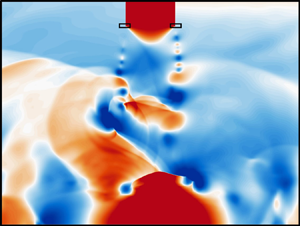
(a) Planar impinging jet domain. (b) Instantaneous uncontrolled pressure snapshot and DMD-ROM initial condition with acoustic probe location. (c) Nozzle forcing location (rectangle) for the DMD-ROM (pressure) and LES (blowing–suction).

As noted earlier, the pressure variable is suitable for the dynamics of interest since it encompasses the hydrodynamic and acoustic phenomena that dictate the feedback loop. A DMD-ROM based on mean-subtracted pressure fluctuations aids in stability by ensuring all DMD eigenvalues are neutrally stable (Towne, Schmidt & Colonius Reference Towne, Schmidt and Colonius2018). A representative baseline pressure snapshot, shown in figure 2(b), illustrates the natural asymmetric (at this time instant, predominantly blue on the right, red on the left outside the stagnation region) side-to-side flapping of the jet and feedback acoustics. The probe location in figure 2(b) monitors the acoustic feedback tones used in the rest of the paper. The forcing is applied on rectangular regions of size  $0.2D \times 0.07D$ centred at the nozzle lip exit, displayed in the inset of figure 2(c), which shows both pressure forcing for the DMD-ROM and blowing–suction actuation for the LES control case.
3.1. Example 1: asymptotic forcing analysis
The first example illustrates the asymptotic tonal response of the forcing model. The power spectral density (PSD) of the uncontrolled pressure fluctuations from the acoustic probe is plotted in figure 3(a). Several tones are evident, the two loudest of which are at  $St=0.2$ and
 $St=0.4$. These correspond respectively to asymmetric and symmetric patterns, consistent with prior studies (Stahl et al. Reference Stahl, Prasad and Gaitonde2022), as elaborated further below. We consider a broad range of forcing amplitude and frequency parameters. To illustrate the capability of the DMD-ROM approach, we first discuss in detail the effect of sinusoidal forcing at a frequency of
 $St=0.4$ and amplitude
 $A=0.005$ (lower part of figure 3b), which is only approximately
 $10\,\%$ of the acoustic fluctuations at the probe. The forcing is applied to both sides of the nozzle exit. These conditions represent the potential manipulation of the resonance mode from the loudest asymmetric tone at
 $St=0.2$ to the symmetric mode at
 $St=0.4$. A short-time comparison of the unforced and forced DMD-ROM probe signals, top part of figure 3(b), displays a gradual deviation of the pressure over time due to the forcing.
(a) Unforced acoustic feedback tones at the probe located outside the jet. (b) Initial deviation of the unforced LES and forced DMD-ROM (top) with the forcing input signal (bottom). (c) Scaled DMD-ROM acoustic spectrogram subtracted from unforced spectrogram. (d) Leading POD mode and temporal coefficient spectra of the unforced and forced systems.

The long-term, asymptotic influence of the forcing on the resonance tones is displayed in figure 3(c) with a spectrogram of the probe signals. To better highlight tonal differences, the DMD-ROM results are normalized by the gain ( $\sigma =1.44$) and subtracted from the unforced spectrogram. This scaling assures a fair relative comparison because, in terms of absolute magnitude, forced linear models tend to increase energy across all frequencies proportional to the gain; this behaviour is discussed further below. The spectrogram differences demonstrate that the
 $St=0.4$ tone increases with time, while the
 $St=0.2$ tone diminishes. Changes to the overall flow field are shown in figure 3(d) by the leading POD modes of the unforced and forced systems, along with their corresponding unscaled temporal coefficient spectra. The results demonstrate that the dominant mode without control is asymmetric at
 $St=0.2$, while that in the forced case is symmetric at
 $St=0.4$. Clearly the forcing resonates with the symmetric impinging mode, which overtakes the nominal flapping mode as the leading dynamic.
To confirm the results from the model, an LES with control is employed by applying perturbations at  $St=0.4$ along the spanwise length of the nozzle using a realizable blowing–suction actuator. As depicted in figure 2(c), actuation is applied on the inner side of the nozzle lip by specifying choked flow based on the main impinging jet nozzle condition. The ratio of the maximum injected mass flow rate to the main jet is
 $\dot {m}_c/\dot {m}_j=0.08$, and facilitates an adequate amplitude response for comparison with the DMD-ROM predicted frequencies. The acoustic probe spectrogram from the controlled LES results is presented in figure 4(a). As in the DMD-ROM, the initially louder
 $St=0.2$ tone diminishes with time and is replaced by the
 $St=0.4$ tone as the forcing dominates the solution. While the frequencies and overall dynamics are predicted favourably, the magnitude of the tones is overpredicted by the DMD-ROM approach. This is a consequence of its linear nature, which precludes nonlinear saturation mechanisms and earlier motivated the gain scaling in figure 3(c) to isolate the observed trends. The leading POD mode and its PSD obtained from the LES are shown in figure 4(b). A comparison with POD modes of figure 3(d) demonstrates a similarity between the controlled LES and DMD-ROM forced results, reflecting the fact that the leading mode is now symmetric, as opposed to the asymmetric unforced case.
Validation of the LES blowing–suction at  $St=0.4$ showing the (a) controlled LES spectrogram and (b) leading POD mode and temporal coefficient spectra.

The gain behaviour is now examined for a range of forcing frequencies and amplitudes. Figure 5(a) shows the gain from  $St=0.03$ to
 $1.1$ and amplitudes
 $A=0.001$ to
 $0.015$. As noted earlier, for this problem, the gain (§ 2) measures the ratio of the
 $L_2$-norm for all forced snapshots to unforced snapshots and therefore captures the asymptotic trends in total energy growth over the time period of the unforced data. Several streaks are observed, corresponding to frequencies amplified by the flow, among which the resonance tones are particularly susceptible and thus prominent. Figure 5(b) selects some of these amplified tones to isolate gain versus forcing amplitude; the previous detailed results at
 $St=0.4$ forcing are marked with a red line. For some forcing frequencies, e.g.
 $St=0.2$ and
 $0.6$, growth is observed at all amplitudes. For others, including
 $St=0.4$, a larger minimum amplitude is required to observe the initiation of gain, after which the gain slope rises linearly on the log–log scale. The behaviour of the
 $\sigma =1$ regime is attributable to perturbation amplitudes that are too low to grow appreciably against the fluctuating snapshots over the finite time period of the snapshots. This has implications on the time required for the forced solution to reach a new observable, asymptotic state. Therefore, for a given number of snapshots, larger amplitudes are preferred for sensitivity studies to better educe relative gain rates (
 $\sigma >1$). On the other hand, some frequencies in figure 5(a) display no realizable gain for all amplitudes, indicating these forcing conditions have little influence on the flow. Of course, forcing characteristics that inhibit pressure fluctuations (
 $\sigma < 1$) are of great interest from a practical perspective, but the present approach, like other linear methods, highlights only growing modes. However, the upcoming transient analysis discusses a method to inhibit growth by interfering with time-local events.
(a) DMD-ROM gain as a function of forcing amplitude and frequency. (b) Forcing amplitude at resonance tones.

3.2. Example 2: transient receptivity analysis
To demonstrate the versatility of the DMD-ROM approach, the statistically stationary fluctuations of the prior example are replaced by a conditional space–time mode that isolates the sequence of acoustic wave arrival followed by growth of the convective shear-layer instability. For this, the DMD-ROM is cast as a transient receptivity analysis subject to external forcing, where the gain is measured over a short time horizon. The CST-POD calculation is derived as described in Stahl et al. (Reference Stahl, Prasad, Goparaju and Gaitonde2023). Briefly, the unforced pressure signal at the probe (shown earlier in figure 2a) is analysed to conditionally identify finite-time events and corresponding snapshots. A few peak amplitudes in the pressure signal are shown in figure 6(a) for reference, representing acoustic waves passing by the probe. Each CST-POD event time window spans  $\Delta T=10$ (
 $100$ snapshots) and is centred between two feedback cycles, capturing
 $74$ total events across the entire dataset to generate the ensemble. A sample event is shown in figure 6(b) with the probe pressure (left axis) plotted with the black solid curve.
(a) Acoustic feedback events from pressure probe. (b) Isolated event from the acoustic pressure signal (black) in comparison to the CST-POD transient gain (shaded) through two feedback cycles. (c) CST-POD mode progression in time.

The CST-POD mode is obtained from a local spatial domain near the nozzle where the events are sampled; a few representative snapshots are depicted in figure 6(c) to highlight the upstream-moving acoustic wave and the ensuing shear-layer instability. The transient gain of the CST-POD mode is normalized by the first CST-POD snapshot and is shown by the shaded curve in figure 6(b), illustrating the timing between the acoustic event ( $t=0$) and peak shear-layer growth (
 $t=+2$) in the feedback cycle. This transient gain represents the baseline for evaluating the flow response to different external forcing parameters.
The DMD-ROM forcing for this example case is similar to the previous case, but is only applied on the nozzle side where the CST-POD mode was derived. Since the CST-POD data are not statistically stationary, both  ${\boldsymbol{\mathsf{U}}}$ and
 $\tilde {{\boldsymbol{\mathsf{A}}}}$ are calculated from the full variable without subtracting the mean. In addition to forcing frequency and amplitude, the phase now becomes an important factor because of the short time horizon. Results using the previous
 $St=0.4$ forcing with an optimal amplitude and phase are first presented before examining the entire parameter space. The choice of the amplitude is arbitrary since it is referenced to the CST-POD mode; in this case
 $A=0.5$ captures the desired trends in the neighbourhood of the local minimum. The optimal phase is
 $\phi =150^{\circ }$ based on the parameter sweep presented below.
Figure 7(a) displays the forcing (lower part of the figure) and gains associated with unforced and forced responses. The results show that the transient gain is significantly reduced at the peak of the shear-layer instability. Figures 7(b)–7(d) illustrate the shear-layer receptivity as a function of forcing phase. In figure 7(b), the transient gain shows phase effects for a constant  $St=0.4$ forcing. At
 $\phi =150^{\circ }$, the forcing influences the natural instability processes and dampens the peak at
 $t=+2$. Figure 7(c) plots the overall gain (
 $\sigma$) as a function of amplitude and phase for
 $St=0.4$. As with the asymptotic case of Example 1, the gain increases linearly with forcing amplitude; this holds for all other frequencies as well. However, in this transient case, conditions where gain is reduced (
 ${\sigma <1}$) become more apparent and are of interest. Figure 7(d) explores the larger parameter space by plotting the overall gain as frequency and phase are varied. As expected, the lower frequencies display the largest modulation in shear-layer instability growth; these are on the order of the resonant frequencies and have fewer cycles within the CST-POD time window. In contrast, higher frequencies have little influence on receptivity and are less affected by phase.
(a) Transient gain of the unforced and forced feedback cycles ( $St=0.4$,
 $A=0.5$ and
 $\phi =150^{\circ }$). (b) Transient gain as a function of forcing phase. (c) Overall gain as a function of phase and amplitude (
 $St=0.4$). (d) Overall gain as a function of frequency and phase (
 $A=0.5$).

4. Discussion
A data-driven framework is presented to discern the linear response of a turbulent flow with a view towards control analyses. The nonlinear system is modelled with a DMD-ROM. Prescribed forcing conditions are projected onto the same reduced space as the unsteady flow, and its effects obtained in the time domain. Computational efficiency is ensured by calculating the gain due to forcing in the reduced subspace, which enables rapid scanning of large ranges of forcing parameters, from which candidates may be expanded to the physical space for further study and verified with scale-resolved methods.
The key advantages of the method are that, being data-driven, it may be applied to any flow field for which time-resolved snapshots are available, regardless of geometry and flow parameters, and without need to solve the linearized Navier–Stokes equations. Furthermore, the time-domain nature of the technique facilitates examination of the forced evolution in the unsteady flow itself, and eases actuator perturbation inputs and examination of transient events where phase becomes important.
Application of the model to the complex physics associated with a resonating supersonic impinging jet, forced at the nozzle receptivity region, successfully predicts the switch from flapping to symmetric resonance modes, as validated with a full three-dimensional, nonlinear simulation. For transient events, the effects of forcing at different phases of receptivity events within the resonant cycle provides guidance on diminishing or amplifying convective instabilities; such phase sensitivities cannot be deduced from the traditional spectral methods. Although the DMD-ROM was implemented here as off-line feed-forward control and validated in the asymptotic sense, these examples advocate for a broader capacity to facilitate time-dependent feedback control, such as the linear phase actuation methods of Illingworth, Morgans & Rowley (Reference Illingworth, Morgans and Rowley2012) in similar resonating systems.
In both examples, thousands of forcing parameters were tested across amplitude, frequency and phase variables, highlighting the performance and utility of the method. For reference, the 2044 parameters tested in Example 1 took approximately 12 h to compute on a single processor compared to the hundreds of hours on 1024 processors for one LES calculation. The DMD-ROM is not limited to harmonic forcing or a single forcing location either. Ongoing research, not shown here, has proven effective in using impulse forcing to pursue convective instabilities at different locations in a boundary layer. Furthermore, the data-agnostic nature of the DMD-ROM has been successfully applied to qualitative measurements of schlieren videos. With a versatile framework for control adaptations, numerous opportunities are available to enhance and apply this method to other problems.
Funding
The authors acknowledge support from the Collaborative Center for Aeronautical Sciences and the Office of Naval Research.
Declaration of interests
The authors declare no conflict of interest.



