2. Flux expression

We consider a closed domain $\mathscr{D}$ consisting of a porous medium with an input source located at $\boldsymbol{x}_{I}$ and an output sink at $\boldsymbol{x}_{O}$ , each with prescribed pressure

with $p_{I}^{\ast }>p_{O}^{\ast }$ . We assume that Darcy’s law holds for an incompressible fluid with velocity $\boldsymbol{u}$ , and so

where we have now non-dimensionalised with respect to the, assumed constant, fluid viscosity and where $\unicode[STIX]{x1D646}$ is a symmetric matrix parameterisation of the, in general anisotropic, permeability. We impose a no-flow condition at the boundary of our domain, i.e.

where $\boldsymbol{n}$ is the outward facing normal vector to the domain boundary. The total flux $Q$ can be written as a limiting integral around the source or the sink,

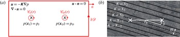
where $\mathscr{C}_{I}(r)$ and $\mathscr{C}_{O}(r)$ are circles of radius $r$ around the source and sink respectively (see figure 1 a). Note that the normal vector $\boldsymbol{n}$ here is pointing towards the source or sink to be consistent in orientation with the domain boundary normal. Using (2.1),

where $p_{I}$ and $p_{O}$ are the non-dimensionalised pressures at the source and sink. By noting (2.3) and then applying the divergence theorem followed by (2.2b ),

where $\partial \mathscr{S}$ is the union of the boundary of $\mathscr{D}$ with $\mathscr{C}_{I}$ and $\mathscr{C}_{O}$ and $\left(\boldsymbol{{\rm\nabla}}p\right)^{\text{T}}$ is the matrix transpose of $\boldsymbol{{\rm\nabla}}p$ . Finally, Darcy’s law yields

Note that (2.7) also holds for an infinite flow domain provided the fluid velocity decays sufficiently rapidly in the far field: $\left|\boldsymbol{x}\right|^{d-1}\boldsymbol{u}\rightarrow \mathbf{0}$ as $\left|\boldsymbol{x}\right|\rightarrow \infty$ , where $\left|\boldsymbol{x}\right|$ is the Euclidean distance from the origin and $d$ is the spatial dimension of the flow domain. We note that in the case of a time-dependent pressure change between the source and sink ${\rm\Delta}p(t)$ , the flux $Q(t)$ is given by $Q(t)={\rm\Delta}p(t)Q\left(t_{0}\right)/{\rm\Delta}p\left(t_{0}\right)$ for any reference time $t_{0}$ . This is because the pressure gradients in (2.7) will scale with ${\rm\Delta}p(t)$ for single-phase flow. For multiple sources and/or multiple sinks the derivation above can be easily adapted to show that for source and sink outflow fluxes $Q_{i}$ and pressures $p_{i}$ , (2.7) becomes

Note that $Q_{i}<0$ for flow into a sink.

Figure 1.

(a) Two-dimensional schematic of a flow domain $\mathscr{D}$ . Source/sink positions are shown by crosses and contours of $\partial \mathscr{S}$ ( $\mathscr{C}_{I}(r)$ , $\mathscr{C}_{O}(r)$ and $\partial \mathscr{D}$ the boundary of $\mathscr{D}$ ) are shown in grey (red online). (b) Schematic of source and sink positions, position parameters $h$ and ${\it\theta}$ , and subdomains (boundaries marked in black) with assigned permeabilities $X_{i}$ and layer height $H$ .

3. Parameter sensitivity

The permeability $\unicode[STIX]{x1D646}=\unicode[STIX]{x1D646}(\boldsymbol{x},{\bf\alpha})$ is, in general, a function of space $\boldsymbol{x}$ and parameters ${\bf\alpha}=\left({\it\alpha}_{1},{\it\alpha}_{2},\dots ,{\it\alpha}_{n}\right)$ . The partial derivative of the flux with respect to parameter ${\it\alpha}_{i}$ gives the dependence of the flux on variations in the parameter ${\it\alpha}_{i}$ , i.e.

using (2.7), with the second term resulting from the symmetry of the integrand. Darcy’s law (2.2a ), the divergence theorem and (2.2b ) yield

as $\boldsymbol{u}\boldsymbol{\cdot }\boldsymbol{n}=0$ on the boundary of $\mathscr{D}$ and the pressure is prescribed and constant $\left(\partial p/\partial {\it\alpha}_{i}=0\right)$ at the source and the sink. Therefore (3.1) becomes

Equation (3.3) can be used to quantify the sensitivity of the flux to changes in parameters within a given model for the permeability provided $\partial \unicode[STIX]{x1D646}/\partial {\it\alpha}_{i}$ can be computed. Examples of such parameters include values of permeabilities at points in space or correlation length scales used within interpolation methods. We will discuss correlation length scales within interpolation methods in more detail in §§ 7 and 8. Use of (3.3) does not require repeated calculation of solutions to the flow (2.1)–(2.3) for many realisations of a varying-permeability field.

A model for the permeability which is widely used (see, for example, Wen & Gómez-Hernández Reference Wen and Gómez-Hernández1996) involves defining the permeability to be spatially constant within finite-size subdomains of the flow domain. The parameters for this spatially discrete permeability field are the values for the permeability on each subdomain, as shown schematically in figure 1(a). The flux is then given by a linear combination of the parameters $X_{i}$ which represent the permeability. We denote by $X_{i}$ the spatially constant value of the permeability in subdomain $\mathscr{D}_{i}\subseteq \mathscr{D}$ as shown in figure 1(b). Equation (2.7) yields

using the Einstein summation convention. With the permeability described by the parameters $X_{i}$ in this way, (3.3) becomes

Thus we see that the integrals $a_{i}$ defined in (3.4) give the magnitude of the sensitivity of the flux to variations in the corresponding permeability parameters.

In order to demonstrate an application of the above results we consider an idealised porous medium. Specifically, we consider a layered system with each of the layer permeability parameters $X_{i}$ set to be equal. That is, the permeability $\unicode[STIX]{x1D646}$ is modelled as spatially constant and isotropic across the entire domain. This is representative of a layered system where the rock properties in individual layers are similar though their deposition is associated with different geological events. We show that the resulting flux derivatives are sensitive to the position of the source and the sink relative to the layer boundaries.

We scale our domain by the distance between the source and sink locations $d$ which we set to be 1. Our flow domain is a $2\times 2$ square. We set each of the layer heights as a constant $H$ . We define the positions of the source and sink by describing the line joining their locations with two parameters: $h$ the displacement of the midpoint of the straight line connecting the source to the sink from the centre of the layer containing this midpoint; and ${\it\theta}$ the angle between the straight line connecting the source to the sink and the layer boundaries, as shown in figure 1(b). 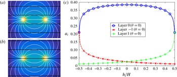Owing to the symmetry of the permeability field, $h/H\in \left[-0.5,0.5\right]$ and ${\it\theta}\in \left[0,{\rm\pi}/2\right]$ describe the range of unique source and sink positions relative to the layered structure. We plot flow streamlines with overlaid layer boundaries shown in black for: $h/H=0$ , ${\it\theta}=0$ , $H/d=0.4$ (figure 2 a) and $h/H=0.5$ , ${\it\theta}=0$ , $H/d=0.4$ (figure 2 b).

Figure 2.

(a,b) Flow streamlines with overlaid layer boundaries shown in black with: (a) $h/H=0,{\it\theta}=0,H/d=0.4$ , (b) $h/H=0.5,{\it\theta}=0,H/d=0.4$ . (c) Variation with sink position $h/H$ of $a_{i}$ (defined in (3.4)) for the central three layers with $H/d=0.4$ and layer orientation ${\it\theta}=0$ .

For a layer angle of ${\it\theta}=0$ and for $H/d=0.4$ , figure 2(c) shows the variation with $h/H$ of $a_{i}$ for the layer in which the source and sink are located (layer 0) and the two adjacent layers (layers $-$ 1 and 1). We see that the $a_{i}$ are sensitive to the position of the source and the sink relative to the layered structure. The central layer (layer 0) has the largest value across the full range of values for $h$ , which is to be expected as layer 0 contains the source and the sink for this value of ${\it\theta}$ (see figure 2 a,b) and thus contains the largest pressure gradients due to the uniformity of the mean permeability $\unicode[STIX]{x1D646}_{0}$ . The value of $a_{0}$ is maximised when $h/H=0$ as here the source and the sink are in the centre of layer 0 (see figure 2 a).

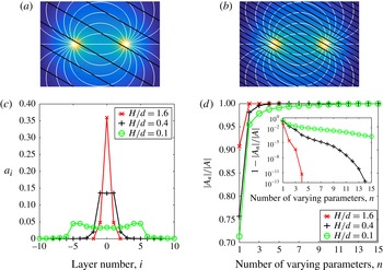
We plot flow streamlines with overlaid layer boundaries in black for: $h=0,{\it\theta}={\rm\pi}/6,H/d=0.4$ (figure 3 a) and $h=0,{\it\theta}={\rm\pi}/6,H/d=0.1$ (figure 3 b). In figure 3(c) we plot $a_{i}$ against layer number for layer heights given by $H/d=0.1$ , $H/d=0.4$ and $H/d=1.6$ . The values are averaged across 101 incremental values of $h/H\in \left[-0.5,0.5\right]$ and across 101 values of ${\it\theta}\in \left[0,{\rm\pi}/2\right]$ . As the ratio of layer height to source/sink spacing $H/d$ decreases, the number of layers spanning the flow domain increases. The total number of layers for $H/d=0.1$ is 57 with the central 21 plotted; the values of the $a_{i}$ outside this range continue decreasing to zero in either direction.

Figure 3.

(a,b) Flow streamlines with overlaid layer boundaries shown in black with: (a) $h=0,{\it\theta}={\rm\pi}/6,H/d=0.4$ , (b) $h=0,{\it\theta}={\rm\pi}/6,H/d=0.1$ . (c) Variation between layers of $a_{i}$ averaged across 101 values of position parameter $h/H\in \left[-0.5,0.5\right]$ and 101 values of layer angle ${\it\theta}\in \left[0,{\rm\pi}/2\right]$ for three different layer heights $H/d=0.1$ , $0.4$ and $1.6$ . (d) The dependence of the proportional flux variation, $|\boldsymbol{A}_{n}|/|\boldsymbol{A}|$ defined in (3.6), on the number of parameters varied when averaged across 101 values of $h/H\in \left[-0.5,0.5\right]$ and 101 values of ${\it\theta}\in \left[0,{\rm\pi}/2\right]$ for $H/d=0.1$ , $0.4$ and $1.6$ .

For $H/d=1.6$ the distribution of the $a_{i}$ is unimodal since the source and the sink both lie within layer 0 for a large range of values in $\left(h/H,{\it\theta}\right)\in \left[-0.5,0.5\right]\times \left[0,{\rm\pi}/2\right]$ due to the large layer height, $H$ , relative to the source/sink spacing, $d$ . However, for $H/d=0.4$ and 0.1, the distribution of the $a_{i}$ becomes bimodal when averaged across ${\it\theta}\in \left[0,{\rm\pi}/2\right]$ . Owing to the small layer height relative to the source/sink spacing, the source and the sink are located in many different layers as ${\it\theta}$ is varied (see figure 3 b). This qualitative change in distribution appears to occur close to $H/d=0.4$ .

Our method can be used to calculate the number of parameters which should be varied within a more computationally intensive nonlinear model. We consider the ‘proportional flux variation’ $|\boldsymbol{A}_{n}|/|\boldsymbol{A}|$ defined as

where $\boldsymbol{A}=\left(A_{1},A_{2},\dots \right)$ is the ordered vector of coefficients $a_{i}$ and $N$ is the total number of layers. $\left|\boldsymbol{A}_{n}\right|/\left|\boldsymbol{A}\right|$ is the ratio of the variation in the flux that results from varying the $n$ most significant of the parameters $X_{i}$ to the flux variation resulting from varying the full set of $X_{i}$ . Figure 3(d) plots $\left|\boldsymbol{A}_{n}\right|\!/\!\left|\boldsymbol{A}\right|$ as a function of $n$ for $H/d=0.1,0.4,1.6$ when averaged across $h$ and ${\it\theta}$ . Figure 3(d) shows that for $H/d=1.6$ , variation in the permeability value of the most dominant layer accounts for a very large proportion of the total variation in flux that results from varying all of the parameters, while decreasing $H/d$ requires more and more layers to account for the same proportion of the total flux variation.

4. Linearised flux sensitivity

We can extend our approach to gain a quantitative estimate of the variance of the flux in the case of small perturbations of the permeability. We write the permeability as the sum of a fixed $\unicode[STIX]{x1D646}_{0}$ and a small perturbation ${\it\epsilon}\unicode[STIX]{x1D646}_{1}$ where ${\it\epsilon}\ll 1$ . ${\it\epsilon}\unicode[STIX]{x1D646}_{1}$ represents the uncertainty in the mean permeability $\unicode[STIX]{x1D646}_{0}$ estimated from available data. We similarly expand the fluid pressure, velocity and flux:

where ${\it\epsilon},{\it\delta}_{u},{\it\delta}_{q},{\it\delta}_{p}\ll 1$ . We include second-order terms to find the sign of the second-order flux correction. The no-flow condition (2.3) applies to both $\boldsymbol{u}_{0}$ and $\boldsymbol{u}_{1}$ on $\partial \mathscr{D}$ . The leading-order pressure $p_{0}$ has boundary conditions at the source and sink given by (2.1), so $p_{i}=0$ at both the source and the sink for all $i\geqslant 1$ .

Darcy’s law (2.2a ) becomes to first order

while (2.7) yields to second order

By definition

and by making the natural scaling assumption, ${\it\delta}_{q}={\it\delta}_{p}={\it\epsilon}$ , and using (4.2), we obtain

We note that the natural scaling assumption ${\it\delta}_{q}={\it\delta}_{p}={\it\epsilon}$ can be shown to be the only non-trivial balance between the terms of (4.2) and (4.3). Finally, with $r$ and $\partial \mathscr{S}$ defined as in § 2, the divergence theorem yields as $p_{1}=p_{2}=0$ at the source and the sink and $\boldsymbol{u}_{0}\boldsymbol{\cdot }\boldsymbol{n}=\boldsymbol{u}_{1}\boldsymbol{\cdot }\boldsymbol{n}=0$ on the boundary of $\mathscr{D}$ . Dropping higher-order terms we obtain expressions for the leading-order change and second-order correction in flux due to the perturbation in permeability:

We note that (4.9a ) is independent of the pressure perturbation ${\it\epsilon}p_{1}$ , a property we shall exploit in a similar manner to § 3. Combining (4.4) and (4.9a ) we see that the total flux $Q$ to first order in ${\it\epsilon}$ is given by

The key difference between (4.10) and the exact expression for the flux (2.7) is that (4.10) does not require the recalculation of the full pressure field $p$ for a change in the permeability, but rather depends only on the leading-order pressure $p_{0}$ . We also note that (4.9b ) is negative definite and so the first-order-in- ${\it\epsilon}$ approximation of the flux is at least a local upper bound for the full nonlinear flux.

We now consider modelling the permeability $\unicode[STIX]{x1D646}$ as a random field. We can use (4.10) to calculate statistical moments of the flux resulting from a probability distribution for the permeability. We consider the parameters $X_{i}$ from § 3 to be independent random variables with constant means ${\it\mu}_{i}$ and variances ${\it\sigma}_{i}^{2}$ , where parameter $X_{i}$ represents the value of the permeability on subdomain $\mathscr{D}_{i}$ . As in § 3 it follows from (4.10) that

where we have once again used the Einstein summation convention. Hence, the expected value $\mathbb{E}$ and variance ${\it\sigma}_{Q}^{2}$ of $Q$ are given by, to first order in ${\it\epsilon}$ ,

It is important to emphasise that the coefficients $a_{0i}^{2}$ are independent of the distribution of the permeability.

Figure 4.

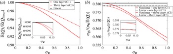
Comparison between linear estimates (black horizontal lines) and nonlinear calculations (grey lines, red online) for (a) the mean flux $\mathbb{E}(Q)$ and (b) the standard deviation of the flux ${\it\sigma}_{Q}$ normalised by the mean flux $\mathbb{E}(Q)$ as a fraction of the standard deviation of the permeability ${\it\sigma}_{\unicode[STIX]{x1D646}}$ . Results derived from example C1 (allowing one layer to vary) and example C3 (allowing three layers to vary) are shown by dashed lines and solid lines using 1000 and 64 000 flux calculations respectively. Insets show behaviour for ${\it\sigma}_{\unicode[STIX]{x1D646}}\in \left[0,0.1\right]$ .

We shall now compare these linear estimates to the nonlinear mean and variance of the flux. We consider each of the permeabilities $X_{i}$ to be log–normally distributed with constant and uniform mean $\unicode[STIX]{x1D646}_{0}$ and standard deviation ${\it\sigma}_{\unicode[STIX]{x1D646}}\in \left[0,1\right]$ . We compute the pressure field $p$ and hence the flux $Q$ for each sample set of values for the $X_{i}$ drawn at incremental percentiles of the assigned log–normal distributions. From these sample flux values we then calculate the nonlinear estimates of the mean and standard deviation for the flux. The sampling is performed using this systematic method in order to resolve the tails of the permeability distributions with the limited number of samples taken. The number of samples is limited by the computational expense of the associated pressure calculations. We also calculate the linear estimates for the mean and standard deviation of the flux as described by (4.11) and (4.12), which only uses the flux value corresponding to $X_{i}=\unicode[STIX]{x1D646}_{0}$ for all $i$ . For this example, we consider the same layered system as described in § 3 with the layer height fixed at $H/d=0.4$ and the source and sink positions relative to the layered structure determined by $h/H={\it\theta}=0$ . For illustration, we consider two simple examples. In example C1 we vary the permeability of the central layer alone, and in example C3 we vary the permeability of the central three layers. All other parameters $X_{i}$ are held constant and equal to $\unicode[STIX]{x1D646}_{0}$ . Without loss of generality, we set $\unicode[STIX]{x1D646}_{0}=1$ .

Figures 4(a) and 4(b) show the comparison between linear estimates, shown by black lines, and nonlinear calculations, shown by grey lines (red online), for the mean flux $\mathbb{E}(Q)$ and the standard deviation of the flux ${\it\sigma}_{Q}$ normalised by $\mathbb{E}(Q)$ and as a fraction of the standard deviation of the permeability ${\it\sigma}_{\unicode[STIX]{x1D646}}$ . In each figure results derived from example C1 are shown by dashed lines and example C3 by solid lines. For example C1 we calculated the flux for 1000 permeability values in this layer, while for example C3 we calculated the flux for $40^{3}=64\,000$ permeability fields, i.e. 40 independent permeability values per layer varied. These sample sizes balance the need for adequate statistical convergence of the nonlinear estimates with the limitations imposed by the computation time required for a large number of pressure calculations. The linear estimates for the mean flux in examples C1 and C3 are equal (figure 4 a) as the mean value of the permeability perturbations are zero in each of the varied layers. As expected, the linear and nonlinear results converge as the standard deviation of the permeability values ${\it\sigma}_{\unicode[STIX]{x1D646}}$ tends to zero (figure 4 b) and the linear expected value for the flux is larger than the corresponding nonlinear values for all values of ${\it\sigma}_{\unicode[STIX]{x1D646}}$ . As ${\it\sigma}_{\unicode[STIX]{x1D646}}$ approaches the size of the base permeability, $\unicode[STIX]{x1D646}_{0}=1$ , the linear estimate becomes invalid. However in the three-layer example C3 the maximum difference between the linear and nonlinear estimates for the mean and normalised standard deviation of the flux is around 9 % and 6 % of the nonlinear mean and standard deviation respectively. It should be noted that the difference between the linear and nonlinear estimates increases between example C1 and example C3. The value of $|\boldsymbol{A}_{n}|/|\boldsymbol{A}|$ in the central layer (i.e. layer 0) is 0.757 and the value in the central three layers (layers $-$ 1,0,1) is 0.996 (see figure 3 d) suggesting example C3 captures almost all of the nonlinear variation in flux. It is worth emphasising that the linear estimate required only one calculation of the pressure field compared with the 1000 and 64 000 pressure calculations required for adequately converged nonlinear results.

5. Non-uniform mean permeabilities

In §§ 3 and 4 we demonstrated results for a uniform mean permeability $\unicode[STIX]{x1D646}_{0}=1$ . We now consider the case where the mean value varies from layer to layer. We set the layer height to be $H=0.4$ . As a canonical example we change the value of $\unicode[STIX]{x1D646}_{0}$ for two neighbouring layers so as to see the effects this has on the sensitivity of the flux to these layers and to the surrounding layers. We set one layer to have mean permeability $\unicode[STIX]{x1D646}_{0,0}=0.1$ (layer 0) and a neighbouring layer to have mean permeability $\unicode[STIX]{x1D646}_{0,1}=10$ (layer 1). All other layers continue to have $\unicode[STIX]{x1D646}_{0,i}=1$ . With non-uniform mean permeabilities we may consider changes in permeability which are equal in absolute size across layers or which scale with the mean permeability of each layer. For equal changes, (3.4) and (3.5) give the corresponding sensitivities of the flux to changes in permeability. For changes in permeability which scale with the mean we scale (3.4) and (3.5) by the mean permeabilities $\unicode[STIX]{x1D646}_{0,i}$ of each layer, i.e.

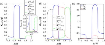
where $\unicode[STIX]{x1D646}_{0,i}$ is the mean permeability of layer $i$ . Equation (5.1) is equivalent to (3.4) and (3.5) for $\unicode[STIX]{x1D646}_{0}=1$ . Figures 5(a) and 5(b) plot the values of $\unicode[STIX]{x1D646}_{0,0}a_{i}/Q$ and $\unicode[STIX]{x1D646}_{0,i}a_{i}/Q$ respectively for the two altered layers (layers 0 and 1) and the two neighbouring layers (layers $-$ 1 and 2). These values are plotted as functions of source and sink position $h/H\in \left[-1.5,2.5\right]$ as defined in § 3 and shown in figure 1(b). This range of values corresponds to the source and sink within each of the four layers in turn.

Figure 5.

(a) Plot of flux sensitivities $\unicode[STIX]{x1D646}_{0,0}a_{i}$ normalised by flux $Q$ for a constant change in permeability across layers. Inset shows values for range $\unicode[STIX]{x1D646}_{0,0}a_{i}/Q\in \left[0,0.1\right]$ . (b) Plot of flux sensitivities $\unicode[STIX]{x1D646}_{0,i}a_{i}$ normalised by flux $Q$ for a change in permeability which is proportional to the mean permeability in each layer. Values plotted for four layers with varying mean permeabilities $\unicode[STIX]{x1D646}_{0,i}$ as shown in the legend. (c) Value of flux $Q$ and linear flux changes ${\it\delta}Q_{a},{\it\delta}Q_{r}$ for constant permeability changes and permeability changes proportional to the mean layer permeabilities respectively. Values plotted as functions of source/sink position $h/H$ as shown in figure 1(b).

The largest value of $\unicode[STIX]{x1D646}_{0,0}a_{i}/Q$ for all $i$ occurs for layer 0 when the source and sink are within this layer. By contrast the values of $\unicode[STIX]{x1D646}_{0,0}a_{1}/Q$ are considerably smaller. This difference in values is because, for changes in permeability which do not scale with the mean value, the relative size of the fluctuation is larger for the low-permeability layer (layer 0) and hence the flux is more sensitive to this layer. Indeed, as highlighted in the inset plot within figure 5(a), $\unicode[STIX]{x1D646}_{0,0}a_{0}/Q$ remains larger than $\unicode[STIX]{x1D646}_{0,0}a_{1}/Q$ even when the source and sink are within layer 1 ( $h/H\in \left[0.5,1.5\right]$ ). From figure 5(b) we note that the largest value of $\unicode[STIX]{x1D646}_{0,i}a_{i}$ for each value of $h/H$ corresponds to the layer containing the source and the sink and that the maximum value attained by each of the $\unicode[STIX]{x1D646}_{0,i}a_{i}$ is approximately equal for each layer. That is, when the permeability fluctuations scale with the mean value, the flux is most sensitive to the layer containing the source and sink and we are in a similar regime to the uniform mean value case $\unicode[STIX]{x1D646}_{0}=1$ from §§ 3 and 4.

Figure 5(c) shows plots of the flux $Q$ and the value of the absolute and relative changes in flux defined as

which correspond to the linear change in flux which results from changes in permeability that are constant across different layers or that scale with the mean permeability of each layer. We see that ${\it\delta}Q_{a}$ is approximately constant as a function of source and sink position $h/H$ . ${\it\delta}Q_{a}$ is approximately equal to $Q$ for $h/H\in \left[-0.5,0.5\right]$ where the source and sink are within layer 0. This is because the change in permeability is here chosen as equal to 0.1 which is equal to $\unicode[STIX]{x1D646}_{0,0}$ , the mean permeability of layer 0. By contrast ${\it\delta}Q_{r}$ is by definition equal to $0.1Q$ and so the percentage or relative change in flux is constant across the range of source and sink positions as suggested in figure 5(b). We would expect our linear estimates to be least accurate for $h/H\in \left[-0.5,0.5\right]$ in the case where the changes in permeability are taken to be constant across layers (where ${\it\delta}Q_{a}$ is the linear change in flux). This is because the change in permeability is comparable in size to the mean permeability in the layer containing the highest pressure gradients.

6. Stochastic simulation

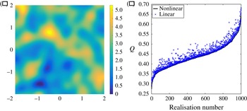
Stochastic simulations can be obtained in a large range of ways, including matrix decomposition techniques (Davis Reference Davis1987), moving average (Black & Freyberg Reference Black and Freyberg1990), nearest neighbour (King & Smith Reference King and Smith1988), spectral methods (Borgman, Taheri & Hagan Reference Borgman, Taheri, Hagan, Verly, David, Journel and Marechal1984) and turning bands (Mantoglou & Wilson Reference Mantoglou and Wilson1982). An elegant method is proposed by Dietrich & Newsam (Reference Dietrich and Newsam1993) which uses a fast Fourier transform method to generate a Gaussian simulation with a controllable correlation length scale. We have used this last method to generate the permeability field shown in figure 6(a). We have chosen a correlation length scale of 0.4 for this simulation with the domain a $4\times 4$ square. This simulation provides a more realistic example of a heterogeneous permeability field than those described in §§ 3–5 and allows us to explore the extent to which the techniques developed in this paper can be applied to such fields. Owing to the stochastic nature of this technique, there is no analytic expression for the derivative of the flux with respect to parameters of the model, for example the correlation length scale prescribed. Hence we cannot use (3.3) directly. However, given multiple realisations of the permeability field, we can apply the linear method from § 4, in particular (4.10), to estimate the associated values of the flux. That is, we calculate the pressure field $p_{0}$ for a chosen reference permeability $\unicode[STIX]{x1D646}_{0}$ and then use (4.10) to calculate the flux $Q$ for a new permeability field $\unicode[STIX]{x1D646}$ . This linear method can be applied to any sample set of permeability fields independently of the technique used to generate them if the change in permeability away from the reference permeability is small by comparison to the reference permeability.

Figure 6.

(a) Permeability field generated using a fast Fourier transform method as proposed by Dietrich & Newsam (Reference Dietrich and Newsam1993), with correlation length $L=0.4$ . (b) Plot of nonlinear flux calculations and linear flux estimates for each of 1000 stochastically generated realisations of permeability with $L=0.4,{\it\sigma}_{\unicode[STIX]{x1D646}}=0.25$ . Data ordered by the value of the nonlinear flux.

We will now apply the linear method from § 4 for sample sets of realisations of the permeability field produced by the methods of Dietrich & Newsam (Reference Dietrich and Newsam1993). The direct output from this method is a field of values normally distributed about zero. In order to produce a positive permeability field one must scale and translate these values. For this example we apply an exponential transformation to the generated fields to produce permeability fields with values given by a log–normal distribution. We choose the scale parameters so that the resulting fields each have mean value equal to 1 and have standard deviations which we will prescribe. Using this algorithm we have generated 16 sample sets each with 1000 permeability fields. Across these 16 sample sets we vary the correlation length scale $L$ and the standard deviation ${\it\sigma}_{\unicode[STIX]{x1D646}}$ of the permeability fields. We use four values for each with $L=0.2,0.4,0.8,1.6$ and ${\it\sigma}_{\unicode[STIX]{x1D646}}=0.25,0.5,0.75,1.0$ . Each sample set of 1000 permeabilities has a unique pair of values for $L$ and ${\it\sigma}_{\unicode[STIX]{x1D646}}$ . We can then assess how the mismatch between linear and nonlinear estimates changes as the standard deviation of the permeability varies for each value of correlation length scale. According to (4.10) we expect differences between the linear and nonlinear estimates for the mean flux to be of order ${\it\sigma}_{\unicode[STIX]{x1D646}}^{2}$ as a fraction of the nonlinear estimate for the mean flux.

Figure 6(b) shows the values of the nonlinear flux and linear estimates of the flux for each of the 1000 permeability realisations with $L=0.4,{\it\sigma}_{\unicode[STIX]{x1D646}}=0.25$ . The values are ordered so that the nonlinear values are monotonically increasing. The nonlinear values are calculated by explicitly solving for the pressure field for each realisation of the permeability. For the linear estimates we calculate the average value of the permeability across the 1000 samples at each point in the flow domain. We then calculate the pressure $p_{0}$ for this average permeability field and use (4.10) to estimate the flux with the permeability $\unicode[STIX]{x1D646}$ given by each of the 1000 realisations in turn. We see that there is some scatter in the linear estimates and that they are all greater than the nonlinear values. 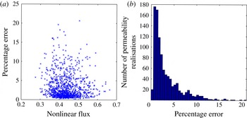The latter characteristic is consistent with the fact that the second-order error term (4.9b ) for the flux is negative. Physically this is because the linear estimate implicitly finds the arithmetic mean of the permeability fluctuations along a given flow streamline. However, the nonlinear flux value results from a combination of geometric and arithmetic averaging of permeabilities. As the geometric average is always smaller than or equal to the arithmetic mean, the linear estimate is always an upper bound. In figure 7(a) we show the percentage difference between the linear estimates and the exact nonlinear flux as a function of the nonlinear flux. The mean nonlinear flux is 0.436. We see that most of the flux values lie between 0.35 and 0.51 with many of the percentage errors significantly below 5 %. The maximum error is about 21 %. Figure 7(b) shows a histogram of the percentage errors with bin size equal to 0.5 %. We see that the majority of the error values do indeed lie below 5 % with a peak between 0.5 % and 1.5 %.

Figure 7.

(a) Plot of percentage error for the 1000 linear estimates for the flux compared to the corresponding nonlinear flux calculation as a function of nonlinear flux with $L=0.4,{\it\sigma}_{\unicode[STIX]{x1D646}}=0.25$ . (b) Histogram of percentage error for the 1000 linear estimates for the flux with $L=0.4,{\it\sigma}_{\unicode[STIX]{x1D646}}=0.25$ and with bin size equal to 0.5 %.

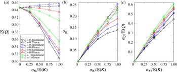
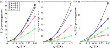
For each of the 16 sets of 1000 permeability realisations we have nonlinearly calculated the mean and standard deviation of the flux. We have then linearly estimated the mean and standard deviation of the flux through use of (4.10). In figures 8(a), 8(b) and 8(c) we plot the values of the mean flux $\mathbb{E}(Q)$ , the standard deviation of the flux ${\it\sigma}_{Q}$ and the ratio ${\it\sigma}_{Q}/\mathbb{E}(Q)$ of the mean and standard deviation of the flux as functions of normalised permeability standard deviation ${\it\sigma}_{\unicode[STIX]{x1D646}}/\mathbb{E}(\unicode[STIX]{x1D646})$ . Figure 8(a) shows that the nonlinearly calculated mean flux decreases as the variability in the permeability fields increases. This is consistent with the interpretation of the nonlinear flux being a combination of the geometric and arithmetic mean of the permeability fluctuations. In contrast the linear estimates for the mean flux do not change by a significant amount as the standard deviation of the permeability ${\it\sigma}_{\unicode[STIX]{x1D646}}$ is increased. In figure 8(b) we see that the nonlinear values and linear estimates for the standard deviation of the flux again diverge for large ${\it\sigma}_{\unicode[STIX]{x1D646}}$ , with the linear estimates maintaining a linear trend with respect to ${\it\sigma}_{\unicode[STIX]{x1D646}}$ . Figure 8(c) illustrates remarkably good agreement between nonlinear and linear estimates for the ratio ${\it\sigma}_{\unicode[STIX]{x1D646}}/\mathbb{E}(\unicode[STIX]{x1D646})$ . Across figure 8(a–c) we see that the nonlinear values of the mean flux $\mathbb{E}(Q)$ , the standard deviation of the flux ${\it\sigma}_{Q}$ and the ratio ${\it\sigma}_{Q}/\mathbb{E}(Q)$ all increase as the correlation length scale increases. This trend is not consistently captured by the linear estimates.

Figure 8.

Plots of nonlinear and linear estimates for (a) the mean flux $\mathbb{E}(Q)$ , (b) the standard deviation of the flux ${\it\sigma}_{Q}$ and (c) the ratio ${\it\sigma}_{Q}/\mathbb{E}(Q)$ of the mean and standard deviation of the flux as functions of normalised permeability standard deviation ${\it\sigma}_{\unicode[STIX]{x1D646}}/\mathbb{E}(\unicode[STIX]{x1D646})$ . Values plotted for correlation length scales $L=0.2$ (circles), $L=0.4$ (squares), $L=0.8$ (triangles) and $L=1.6$ (diamonds). Nonlinear estimates shown by full lines and linear estimates by dashed lines.

In figures 9(a) and 9(b) we plot the percentage differences between exact nonlinear values and linear estimates for the mean flux $\mathbb{E}(Q)$ and standard deviation of the flux ${\it\sigma}_{Q}$ respectively. Values are plotted as functions of permeability standard deviation ${\it\sigma}_{\unicode[STIX]{x1D646}}$ and the four lines in each figure correspond to different values of correlation length scale $L$ . As expected, we see that the difference between the nonlinear and linear estimates increases as the standard deviation of the permeability fields increases. The differences between the estimates also increase as the correlation length $L$ decreases for both the mean and the standard deviation of the flux. We interpret this effect as being a consequence of the fact that for small correlation length scales there are more permeability fluctuations in series along a flow streamline. The nonlinear calculation for the flux accounts for the geometric averaging of the permeability along the streamline while the linear estimate only takes the arithmetic mean.

Figure 9.

Plots of percentage differences between nonlinear and linear estimates for (a) the mean flux $\mathbb{E}(Q)$ , (b) the standard deviation of the flux ${\it\sigma}_{Q}$ and (c) the ratio ${\it\sigma}_{Q}/\mathbb{E}(Q)$ of the mean and standard deviation of the flux as functions of normalised permeability standard deviation ${\it\sigma}_{\unicode[STIX]{x1D646}}/\mathbb{E}(\unicode[STIX]{x1D646})$ . Values plotted for correlation length scales $L=0.2$ , $0.4$ , $0.8$ and $1.6$ .

Figure 9(a,b) shows that as the standard deviation of the permeability increases beyond 0.5 we see significant differences between the linear estimates and the nonlinear values for the statistics of the flux. However the linear estimates and nonlinear calculations for the fractional uncertainty of the flux ${\it\sigma}_{Q}/\mathbb{E}(Q)$ are in good agreement as shown in figure 9(c). We again observe an increase in the difference as ${\it\sigma}_{\unicode[STIX]{x1D646}}$ increases. However, even for $L=0.2$ and ${\it\sigma}_{\unicode[STIX]{x1D646}}/\mathbb{E}(\unicode[STIX]{x1D646})=1$ the error is less than 15 %. This is due to cancellation of the errors shown in figure 9(a,b). The linear estimates for the mean and the standard deviation are both higher than the nonlinear estimates and hence we see the reduced error in figure 9(c). However we encourage caution when applying the linear estimates for standard deviations of permeability above 0.5 as the differences between nonlinear and linear values for the mean and standard deviation of the flux are large.

7. Kriging

Kriging was first proposed as an interpolation method by Krige (Reference Krige1951) and subsequently promoted and developed by Matheron (Reference Matheron1971). It is described as the ‘best linear unbiased estimator’ (‘BLUE’) where ‘best’ means that this technique gives the linear estimator with the minimal error variance whilst remaining unbiased. The extent to which kriging is the best interpolation method to use in any given situation is beyond the scope of this paper. We use kriging merely as an example of a widely used linear interpolation method. The strategies employed below can be similarly applied to any linear regression model used to estimate the permeability.

Kriging is a linear interpolation method used to estimate the permeability $\unicode[STIX]{x1D646}$ at point $\boldsymbol{x}_{0}$ given the values of the permeability at sample points $\boldsymbol{x}_{i}$ . The estimate $\unicode[STIX]{x1D646}(\boldsymbol{x}_{0})$ is taken as a linear combination of the sampled values $\unicode[STIX]{x1D646}(\boldsymbol{x}_{i})$ with weights $w_{i}$ ,

The weightings in (7.1) are given by the ordinary kriging equations

where ${\it\lambda}$ is a Lagrange multiplier and $C_{ij}=\text{Cov}(\boldsymbol{x}_{i},\boldsymbol{x}_{j})$ is the covariance of the permeability at the pair of points $\boldsymbol{x}_{i},\boldsymbol{x}_{j}$ . The covariances $C_{ij}$ will depend upon the correlation length scale $L$ of the covariance model. To calculate the sensitivity of the flux $Q$ to changing the correlation length scale $L$ we can calculate the derivative $\text{d}Q/\text{d}L$ , which from (3.3) is given by

Further, $\partial \unicode[STIX]{x1D646}/\partial L$ is given by

where $\text{d}w_{i}/\text{d}L$ can be estimated by perturbing $L$ and recalculating $w_{i}$ or can be found directly through use of

To derive (7.5) we have used the identity

for the derivative of a matrix inverse. Use of (7.6) allows us to calculate the derivative of $\unicode[STIX]{x1D648}^{-1}$ without calculating $\unicode[STIX]{x1D648}^{-1}$ symbolically. To demonstrate the use of these results in practice we shall use the permeability field shown in figure 6(a) as a surrogate truth model. For the field shown in figure 6(a) we have set the minimum permeability equal to machine precision above zero and specified a standard deviation equal to 1. This choice of value for the minimum permeability was selected so as to give a large range of permeabilities compared with the minimum permeability value. This should yield a demanding test for our linear methods.

In practice the true permeability field is not usually known and to estimate the permeability one must interpolate from a limited amount of sampled points. We will suppose we have measured the permeability at fixed locations from which we will estimate the permeability through kriging. Given the permeability data at the sample locations, the correlation length scale can be estimated using the maximum likelihood estimator

where $n$ is the number of sample locations, $\left|\unicode[STIX]{x1D64D}\right|$ is the determinant of the matrix of covariances (that is $\left(\unicode[STIX]{x1D64D}\right)_{ij}=C_{ij}$ ) and ${\it\sigma}^{2}$ is the process variance given by

where $\boldsymbol{Y}$ is the vector of permeability values at the sample locations and $\boldsymbol{F}^{\text{T}}=\left(1,\dots ,1\right)$ with ${\it\beta}^{\ast }$ given by

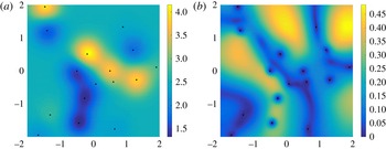
(See Lophaven, Nielsen & Søndergaard Reference Lophaven, Nielsen and Søndergaard2002 for a more thorough discussion of this maximum likelihood estimation.) For this example we have $m=16$ sample locations, with one at each of the source ( $x=\left(-0.5,0\right)$ ) and sink ( $x=\left(0.5,0\right)$ ) and the remaining fourteen randomly located throughout the $4\times 4$ flow domain. The sample locations are shown by the black dots in figure 10(a,b). With these locations and associated permeability data the maximum likelihood estimate of the correlation length is $L^{\ast }=0.3953$ , which is very close to the correlation length scale of 0.4 used in the surrogate permeability (figure 6 a). For this length scale and a Gaussian correlation function the kriged permeability field is shown in figure 10(a). This estimation conserves some of the features of the surrogate permeability field, though owing to the limitations of kriging and interpolation in general, many of the features are lost. Notably, the range of permeabilities has been reduced from approximately $\left[0,5\right]$ to approximately $\left[1.5,4\right]$ . Although it is noteworthy that this loss of information is likely to influence the estimated flow quantities, the failings of interpolation to characterise the surrogate permeability fully are not the focus of this paper.

Figure 10.

(a) Kriged permeability estimated from (7.1) and (7.2) with correlation length scale $L^{\ast }=0.3953$ . (b) Standard deviation of permeability as a fraction of the base field (shown in (a)) as a function of location as the correlation length scale is varied across $\left(L^{\ast }/4,4L^{\ast }\right)$ . Data sample locations shown by black dots.

To analyse the sensitivity of the flux to changes in correlation length we vary the correlation length across 1001 values within $\left[L^{\ast }/4,4L^{\ast }\right]$ . For each value we calculate the associated kriged permeability field. Figure 10(b) shows the standard deviation of the permeability normalised by the permeability values given in figure 10(a). That is, figure 10(b) shows by how much the permeability varies as the correlation length scale is varied. To apply the techniques detailed in §§ 3 and 4 we hope for the standard deviation to be small relative to the mean, which in figure 10(b) corresponds to values which are small compared with 1. We can expect a significant error when estimating the flux if there are locations in the domain where the permeability values have standard deviation approaching or greater than 1, especially if this occurs in close proximity to the source or the sink where the pressure gradients are highest. Figure 10(b) shows that the standard deviation of the permeability is less than the value of the reference permeability across the domain. Most of the domain shows a deviation of around or below 0.4, with a couple of locations with higher variability. From this diagnostic figure we can predict that the error in our linear flux estimates will be small given that the locations of high variability are towards the edges of the flow domain where we expect lower pressure gradients.

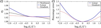
The nonlinear approach to calculating the flux for each sample of the permeability field requires calculation of the pressure field from (2.2) for each permeability realisation. However, using (4.10) we can gain an estimate for the flux resulting from each different permeability with only one pressure calculation, similarly to § 4. The nonlinear results are shown in figure 11(a) by the dashed line while the linear estimate is shown by the full line. We have restricted the maximum value of the $x$ -axis, as for higher correlation length scales some areas of the permeability field become negative. This is both unphysical and changes the equation for the pressure field,

from an elliptic equation to a locally hyperbolic equation resulting in an ill-posed problem.

Figure 11.

(a) Predicted flux against kriging correlation length scale (shown on log scale) from fully nonlinear calculations (dashed line), linear flux calculation (full line) and flux gradient calculation (dotted line). (b) Percentage difference between nonlinear calculation and linear flux (full line) and flux gradient (dotted line) against kriging correlation length scale (shown on log scale).

We can also gain an estimate for the change in flux with respect to correlation length through the use of the gradient given by (7.3)–(7.5). This is shown by the dotted line in figure 11(a). As expected, the linear and gradient estimates both agree with the nonlinear result for $L=L^{\ast }$ and the full line lies entirely above the dashed line, consistent with the fact that the second-order error term (4.9b ) for the flux is negative. That is, the linear estimate for the flux is an upper bound for the value of the nonlinear flux. Figure 11(b) shows the percentage difference between the two estimates used and the nonlinear values for the flux. Encouragingly, this difference is below 2.5 % even for a factor of four change in the correlation length scale. In this example the gradient estimate agrees more closely with the nonlinear calculation though this is not observed to be a general trend.

8. Imposing positive permeability

An issue that arises when using kriging is that the kriging method does not include any constraint on the resulting estimated values. When estimating a positive quantity such as permeability this can lead to negative or otherwise unphysical values as observed in § 7. There are several techniques that have been proposed to impose positivity constraints on the estimated values. Some involve removing negative weights after solving the ordinary kriging equations (7.2) (see, for example, Deutsch Reference Deutsch1996). A technique developed by Kostov & Dubrule (Reference Kostov and Dubrule1986) incorporates the constraints on the values to be estimated within the interpolation procedure. The permeability at the location of the estimate is written as

where the weights $b_{i}$ are to be determined and where $\bar{K}$ is a trend model which we take here to be the mean value of the sampled permeability data. We impose the following constraints:

where $k_{i}$ is the sampled value of the permeability at the sample location $\boldsymbol{x}_{i}$ , $n$ is the number of sample locations and $m$ is the number of points at which we wish to estimate the permeability. Kostov & Dubrule (Reference Kostov and Dubrule1986) propose that the weights $b_{i}$ in (8.1) can be taken as the solution to where $\boldsymbol{b}=\left(b_{1},\dots ,b_{n+m}\right)$ and $\boldsymbol{B}^{\text{T}}=\left(K_{1},\dots ,K_{n},0,\dots ,0\right)$ . One justification for the form of (8.3a ) is the equivalence with the kriging equations (7.2) when the positivity constraints (8.2b ) are removed. The gradient of the flux $\text{d}Q/\text{d}L$ given by (7.3) can again be calculated for this interpolation technique through use of

By defining $f=\boldsymbol{b}^{\text{T}}\unicode[STIX]{x1D64D}\boldsymbol{b}-\boldsymbol{B}^{\text{T}}\boldsymbol{b}$ we can calculate $\partial b_{i}/\partial L$ by noting that the change in the minimum of $f$ will be given by

where the $\boldsymbol{{\rm\nabla}}$ operator is with respect to $\boldsymbol{b}$ .

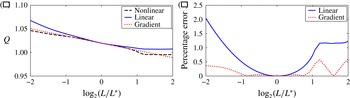
Similarly to § 7 we vary the correlation length across 101 values within $\left(L^{\ast }/4,4L^{\ast }\right)$ . The reduction in the number of simulations in comparison to § 7 is due to the increased computation time for each realisation of the permeability. The results of the nonlinear (dashed line), linear (full line) and gradient (dotted line) estimates for the flux are shown in figure 12(a) and the percentage differences between the linear (full line)/gradient (dotted line) and the nonlinear values are shown in figure 12(b). Once again the linear and gradient estimates agree well with the nonlinear flux values. The flattened behaviour in figure 12(a) of the nonlinear and linear flux values for large values of correlation length scales $L$ arises when the positivity constraints (8.2a ) impose a different permeability estimate to that which would be attained by the kriging equations (7.2).

Figure 12.

(a) Predicted flux against correlation length scale (shown on log scale) from fully nonlinear calculations (dashed line), linear flux calculation (full line) and flux gradient calculation (dotted line). (b) Percentage difference between nonlinear calculations and linear flux (full line) and flux gradient (dotted line) against correlation length scale (shown on log scale).