

I
Minsky and Kindleberger argue that financial crises commonly develop through financial instability in different phases (Minsky Reference Minsky, Kindleberger and Laffargue1982). First, markets lose their long-term equilibrium through significant shocks, causing the economy to run faster. Positive expectations cause the demand for credit to increase. Financial stability is lost, and credit bubbles arise. The economy becomes overheated, and asset bubbles are created. When markets turn, they face credit crunches, asset crashes and recessions (Kindleberger and Aliber Reference Kindleberger and Aliber2005, pp. 33–76). In their empirical studies of international financial crises, Tornell and Westermann conclude that financial liberalization often causes boom–bust cycles (Tornell and Westermann Reference Tornell and Westermann2005).
This article offers an anatomy of Norwegian financial crises as it seeks to answer three questions:
1. When was Norway hit by substantial financial crises between 1830 and 2010?
2. Do financial crises coincide with significant contractions in the real economy?
3. Have credit and money cycles been consistent with the Minsky–Kindleberger approach to financial crises?
In answering these questions, we first trace a chronology of financial crises. Second, we map co-movements of output gaps and key financial indicators. Third, we study developments in credit volume and money stock relative to financial crises.
II
Financial crises refer to situations in which financial institutions or assets lose value significantly. Goldsmith (Reference Goldsmith1982) defines a financial crisis as:
a sharp, brief, ultra-cyclical deterioration of almost all financial indicators, short-term interest rates, asset prices, commercial insolvencies and failure of financial institutions.
Kindleberger claims that financial crises often follow a succession of phases: exogenous shocks, speculative manias, financial distress and economic meltdown (Kindleberger and Aliber Reference Kindleberger and Aliber2005, pp. 1–20). During the nineteenth century and the first part of the twentieth century, financial crises were associated with bank panics and credit crunches. The modern understanding of financial crises includes stock market crashes, financial bubble bursts, currency crises and sovereign defaults.
Drawing on established definitions, we understand financial crises to be significant negative development in several financial indicators, causing credit markets to work irrationally by not providing necessary credit to the economy.
III
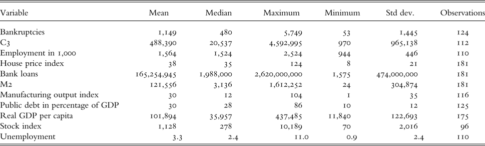
In our work, money stock, credit volume, bank loans, house prices, bankruptcies, stock prices, GDP, manufacturing output, unemployment and public finances are drawn from a project on Historical Monetary Statistics that is monitored by the Norwegian central bank.Footnote 1 The primary data are collected from rich and informative public and private records hosted by Statistics Norway, the central bank, the National Archive, regional archives and the Wedervang Archive at the Norwegian School of Economics. Both the sources of data and the construction of the time series are well documented and must be considered valid and reliable for our purpose. They have been consulted by both domestic and foreign experts (Eitrheim, Klovland and Qvigstad Reference Eitrheim, Klovland and Qvigstad2004, Reference Eitrheim, Klovland and Qvigstad2007).
M2 is the broad money stock. C3 is defined as total credit to the general public. Bank loans are loans from private banks. Observations on the number of bankruptcies cover registrations by local courts all over the country. The house price index is a repeated sales index covering the main cities from the early 1800s until the 1970s and the entire country thereafter. The historical stock price index represents all stocks reported on the Oslo Stock Exchange from 1914 onward. GDP and manufacturing are calculated from the production side on the basis of output and input statistics. Unemployment is extracted from labour market statistics, and public finances, from the ministry of finance.
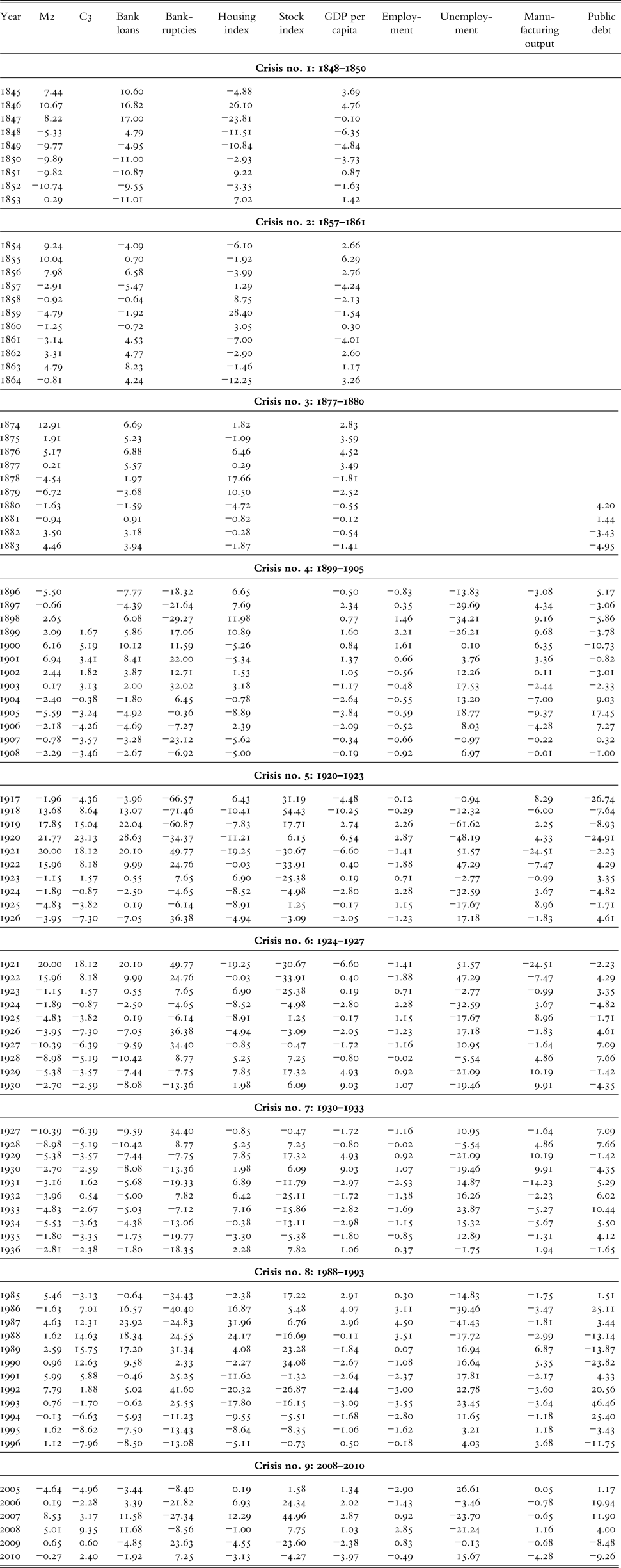
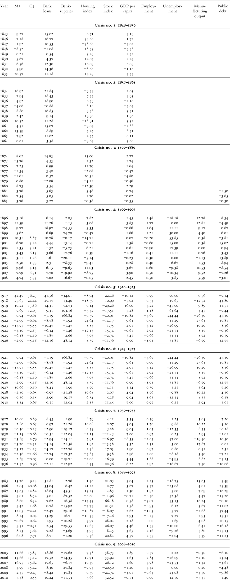
We address the data in two ways. First, we look at the percentage deviation of the observed time series from estimated trends (Table 1).Footnote 2 Second, we present annual percentage changes (Table 2).
Economic variables and financial crises. Percentage deviation from trend

Economic variables and financial crises. Percentage annual changes
IV
By holding existing literature up against financial indicators, we find that nine episodes may fall into our definition of financial crisis.Footnote 3
Crisis no. 1: The revolutionary crisis, 1848–1850
Global impact
The first significant financial crisis that we address occurred in about 1848. From the mid 1840s, continental Europe experienced a huge increase in prices of crops and potatoes. This was due to both supply- and demand-side shocks. First, years of poor harvests increased prices. Second, the Corn Laws, protecting domestic producers, were abandoned in the UK, and a substantial rise in demand for crops in international markets occurred. From early 1845 until the spring of 1847, prices of rye and wheat in continental Europe doubled. Working-class families used 50 per cent or more of their income on agricultural products in most of Europe (Merriman Reference Merriman1996, pp. 718–24). With increasing prices on demand-inelastic food, demand for industrial products fell. The industrial sector experienced a negative demand shock, leading to bankruptcies and credit crisis.
The problems contributed to political discontentment and revolutionary waves sweeping over continental Europe. In France, the monarchy was abolished under the February Revolution of 1848. Uprisings occurred in Italy, Austria–Hungary and Prussia. Uncertainty decreased international trade. Financial markets struggled under a lack of trust and liquidity. In Austria–Hungary, political control was not regained until 1851, while the monarchy was re-established in 1852 in France (Tocqueville Reference Tocqueville1893; Bideleux and Jeffries Reference Bideleux and Jeffries1998, pp. 295–6).
Domestic impact
As for Norway, a lack of confidence in its currency led to a decrease in the silver reserves kept by the central bank from 1846. The negative shift in international demand caused exports to drop and the silver reserves to shrink even further. Thus, the monetary policy had to be tight (Rygg Reference Rygg1918, pp. 289–308).
To avoid further loss of capital, silver redemption was suspended in the central bank's regional offices in Bergen and Oslo when the interest rates were raised at the headquarters in Trondheim (Hodne and Grytten Reference Hodne and Grytten2000, pp. 216–17). Credit granted was radically reduced. Insolvencies and bankruptcies became daily affairs.
At the same time, the real-estate market crashed after huge growth in asset prices until 1847. The crisis also had substantial spillover to the real economy, with a significant contraction of the business cycle.
The problems ended after the government was granted a loan of 0.6 million speciedaler in London and thereafter a 1.5 million speciedaler long-term loan at Hambo's in Denmark.Footnote 4 Shock waves, however, had an impact for another couple of years.
Crisis no. 2: The Crimean crisis, 1857–1861
Global impact
Another crisis hit the world economy after the Crimean War, October 1853 to February 1856. The war was fought between Russia on one side and an alliance of the United Kingdom, France, the Ottoman Empire and the Kingdom of Sardinia on the other. It was officially triggered by interests of control over the Holy Sepulchre in Jerusalem. The more important underlying reason was the contest between the major European powers for influence over the territories of the declining Ottoman Empire. Most combat took place on the Crimean Peninsula, which the Russians had conquered from the Ottomans in 1774 and annexed in 1785.
The immediate impact on international demand was chiefly positive. The demand for services by the merchant fleet increased, and the freight rates rose substantially (Klovland Reference Klovland2009, pp. 266–84). The upheaval was fueled by a gold rush in California. The growth in business activity largely resulted from growth in the short-term credit volume. Speculative bubbles emerged owing to the expectation that prices on exported and imported goods would increase (Calomiris and Schweikart Reference Calomiris and Schweikart1991, pp. 807–34).
After the war, prices fell considerably. Speculators ran into heavy losses. Ship owners and importers with large stocks of rye and wheat, which were purchased at high costs, were losers.
Domestic impact
As merchants and ship owners along the coast of Norway were heavily involved in speculation, the crises were a major blow for them. In Bergen alone, 88 traders and investors went bankrupt between 1856 and 1859 (Hodne and Grytten Reference Hodne and Grytten2000, pp. 157–68).
At first, many merchants and investors were saved by blanco credits granted in Hamburg and London. However, when an international financial crisis began to spread globally from New York during the spring of 1857, financial centers were devastated. Almost 60 percent of the most important short-term creditors for Norwegian companies in Hamburg had to cease their activities. Other creditors demanded rapid cash redemption of their loans. In addition to a serious credit crunch, real-estate prices stagnated after a booming decade.
The government and the newly established bank Den norske Creditbank joined forces in order to avoid financial panics and a stop in the credit market. Guarantees were given, and 320 foreign creditors with claims on 900 Norwegian companies were paid the equivalent of 1.65 million speciedaler. In 1858, the parliament approved a loan from Hambro & Son, London, of 3.6 million speciedaler in foreign currency.
During the late summer of 1858, most of the financial difficulties ceased, but the problems returned with new strength in Bergen (Seip Reference Seip1957, pp. 513–38). The negative effects on industrial output lagged somewhat behind those of the financial markets and were probably at their worst during winter of 1860–1. Real-estate prices stagnated in the late phase of the crisis and fell until 1862.
Crisis no. 3: The long depression, 1877–1880
Global impact
The long depression reflects a series of depressive tendencies in the world economy from the mid 1870s until the early 1890s. Several international financial panics occurred, e.g. 1873, 1882, 1890 and 1893. The depression is considered part of a relative British decline (Musson Reference Musson1959, pp. 199–228; Davis Reference Davis2006, pp. 103-21). The international economy was flourishing under British leadership from 1850 to 1873 (Church Reference Church1975). Interest rates were low, international investments grew rapidly and monetary expansion was substantial.
In the 1870s, international adoption of the gold standard considerably increased the international demand for gold. Thus, gold currencies appreciated relative to silver currencies. Consequently, they lost competitive power, and negative capital movements occurred. Asset bubbles turned into crashes.
Bordo and Meissner show that high debt in hard foreign currencies both transmitted and fueled the crisis. In times of depreciation pressure, it was difficult to defend national currencies. Debt service in gold became increasingly difficult. External funding dried up, and the economy contracted (Bordo and Meissner Reference Bordo, Meissner, Edwards, Esquivel and Márquez2007, pp. 139–94).
Domestic impact
A large monetary expansion occurred within a few years before the crisis. Dependent on trade with the UK, Norway suffered considerably. The per capita real GDP level of 1876 was not reattained until 1888 (Grytten Reference Grytten, Eitrheim, Klovland and Qvigstad2004a, pp. 241–88). It took 38 years for prices to return to their 1874 level (Grytten Reference Grytten2004c, pp. 61–79).
According to county reports, the economy saw a strong boom from 1871 to 1873, with ‘fairytale’ profits. Then, from 1874 to 1875, the dawn of a correction was reported. However, huge public investment and favorable harvests in agriculture and fisheries made 1876 the peak year of GDP.
In July 1869, the key interest rate of the central bank was 5.5 percent. During the following boom, it stabilized below 4 percent between 1871 and 1873 (Klovland Reference Klovland, Eitrheim, Klovland and Qvigstad2007). From January 1869 until January 1874, the money supply increased by more than 53 percent (Klovland Reference Klovland, Eitrheim, Klovland and Qvigstad2004b). Thereafter, Norway experienced two significant contractions from 1876 to 1879 and from 1887 to 1888 (Klovland Reference Klovland1989, pp. 24–31).
Norway, Denmark and Sweden adopted the gold standard earlier than most other countries, with Sweden and Denmark adopting the standard in 1873 and Norway, in 1874. To protect the krone, interest rates were raised from 3.5 to 7.0 percent between 1872 and 1877. From January 1874 to January 1879, the money supply contracted by 28 percent.
Another important reason for the poor performance was the late transition from sail to steam in the merchant fleet (Fischer and Nordvik Reference Fischer, Nordvik, Fischer, McInnis and Schneider1986). Substantial capital was invested in vessels constructed for timber freight. European imports of timber fell during the downturn, and the Norwegian merchant fleet was devastated. Several banks went bankrupt, particularly in the very south of the country, where the merchant fleet was a dominant economic factor. In Arendal, the second largest city in the area, three out of four banks went bankrupt during a local crash in 1886 (Johnsen Reference Johnsen1998).
Crisis no. 4: The Kristiania crisis, 1899–1905
The next crisis was limited to the domestic economy. It was a combination of a credit and private estate crisis from the fall of 1899 until 1905, with considerable effects on the real economy.
When the gold standard was introduced in January 1874, parliament had decided to maintain the quotient system. According to this system, there had to be a minimum ratio between the metal reserves controlled by the central bank and the volume of issued notes. This quotient was set to 2:5. The system was procyclic, as the central bank ran a deflationary monetary policy when metal coverage was low.
The system was abandoned in 1893, and a different system was introduced. With this system, parliament could decide to issue excess notes independent of the metal coverage. This system allowed for less rigid monetary policy and low interest rates. At the same time, agriculture saw rapid growth in productivity, and labor was transferred to the rapidly growing manufacturing industry in urban areas (Søbye Reference Søbye1999; Gerdrup Reference Gerdrup2003). From 1890 until 1899, the population of Kristiania alone increased by 47 percent.
Demand for property increased dramatically. New buildings were financed by cheap credit. In February 1894, the money base (M0) was 53.8 million NOK. By September 1899, it was 86.7 million, an increase of more than 61 percent over 5.5 years (Klovland Reference Klovland, Eitrheim, Klovland and Qvigstad2004b). Wages rose substantially, and house prices increased by 40–70 percent in the major cities during the same period (Eitrheim and Erlandsen Reference Eitrheim, Erlandsen, Eitrheim, Klovland and Qvigstad2004).
The expansion in the private estate market resulted from huge stock issues. (Knutsen Reference Knutsen2007). Six new commercial banks were established in the city between 1896 and 1898, which specialized in high-risk loans. All of these banks went bankrupt during the subsequent crash.
In late 1898, markets became nervous, and in 1899, the bubbles crashed. Prices of property fell considerably – 59 percent in Kristiania from 1899 to 1904 and 43 percent in Bergen from 1898 to 1905. The annual number of bankruptcies increased from 241 in 1890 to 736 in 1903 (Eitrheim and Erlandsen Reference Eitrheim, Erlandsen, Eitrheim, Klovland and Qvigstad2004, pp. 372–5).
Crisis no. 5: The postwar depression, 1920–1923
Global impact
At the start of World War I, gold redemption of currencies was postponed and inflationary monetary policy was monitored to tackle financial challenges. Central bank rates were low, credit volumes increased and states ran fiscal deficits (Romer Reference Romer1988). At the same time, supply was limited because of the war.
A substantial increase in money and higher product demand, in combination with a decrease in supply, led to money accumulation. Inflation skyrocketed, and most currencies depreciated compared with their gold values.
When the war ended and supply increased, the accumulation of money during the war led to a short and hectic boom until the late summer of 1920. By that time, Europe was struggling owing to huge fiscal problems.
The boom was transformed into a severe bust at the same time as governments had to reduce spending and tighten monetary policy. This led to huge financial problems, including bank and currency crises. A classical postwar boom–bust cycle occurred. GDP per capita fell by more than 15 percent in the UK. In Germany and several Eastern European countries, uncontrolled monetary expansion resulted in hyperinflation and economic meltdown.
Domestic impact
The money stock increased by a factor of five in Norway from 1914 to 1920. Thus, demand shifted outward when supply shifted inward. Hence, consumer price inflation skyrocketed, increasing by 207 percent from the outbreak of the war until the late summer of 1920. The krone depreciated by 50 percent from just before the war ended until the autumn of 1920 (Hodne and Grytten Reference Hodne and Grytten2002, pp. 93–116).
Investments increased by 34 percent in two years from 1918 until 1920. Imports were more than double exports in 1919 (Grytten Reference Grytten, Eitrheim, Klovland and Qvigstad2004a, pp. 274–85). Finally, during the late summer and autumn, the markets turned rapidly.
Along with the international recession, the central bank decided to adopt a deflationary monetary policy to bring the krone back to its par value in gold. Thus, the currency had to appreciate by 100 percent. The deflationary policy was monitored in two phases. The first started in the autumn of 1920.
Strong inflation turned into hard deflation as nominal interest rates were increased and credit from the central bank was reduced. Real interest rates peaked at close to 40 percent in the early 1920s. Investments were cut in half. Unemployment rates and bankruptcies reached all-time highs. Bank failures reached 7 percent of GDP in 1923 and 1925, by far the highest losses ever in Norway. The development forced the central bank to halt the deflationary policy during the spring of 1923 (Hanisch, Søilen and Ecklund Reference Hanisch, Søilen and Ecklund1999, pp. 63–90).
Crisis no. 6: The parity crisis, 1924–1927
Global impact
During the 1920s, governments chose different strategies to stabilize their currencies. Germany, Poland, Austria, Hungary and the Soviet Union adopted new currencies. Estonia, Romania, Bulgaria, Portugal, Greece, Yugoslavia, Finland, Belgium, Czechoslovakia, France and Italy devalued their currencies. Finally, the UK, the US, Canada, Japan, the Netherlands, Switzerland, Sweden, Denmark and Norway returned to their prewar gold parities.
Eichengreen concludes that the European countries clinging to the par gold value their currency struggled with overvalued currencies and, thus, low international trade volumes, as well as deflation and contracting domestic demand. This resulted in limited growth and capital flows, high unemployment rates, and bank failures. Countries that were able to restore the par value of their currency or that devalued their currency implemented more inflationary monetary policy, leading to higher demand and growth rates, lower unemployment and thriving financial markets (Eichengreen Reference Eichengreen1990, pp. 24–56).
Domestic impact
During a suspension of deflationary monetary policy in 1923 and 1924, foreign trade was revived, the heavy deficits ceased and unemployment fell. This allowed for a new period of deflationary policy. From late 1924 until May 1928, the Norwegian krone rose toward its par value. The consequence was again financial contraction and a stagnant economy, with more than a hundred bank failures. Economy-wide unemployment reached more than 8 percent on an annual basis.
The depressions of the 1920s stand out as the worst financial crises recorded in Norway. According to national accounts, only the UK was hit harder in the early 1920s, after which Norway performed even worse during the mid 1920s.
As for this crisis, the time series reveal a credit crunch. This is translated into a decline in housing prices and the real GDP per capita. In 1926, there was also a large increase in the number of bankruptcies. The stock market was also negatively affected by the domestic monetary policy.
Crisis no. 7: The Great Depression, 1930–1933
Global impact
An international boom from the mid 1920s was transformed into the strongest global depression recorded in modern history. The downturn started when the overheated economy collapsed in the US from October 1929.
International financial instability gave the US and France huge capital inflow in the 1920s. One source was war reparations paid by Germany to France and Belgium; another was inter-allied debt paid from European allied powers to the US. In addition, both the US and France had undervalued their currencies and were protectionists. As a consequence, they accumulated capital, when most of Europe lost liquidity and was dependent on short-term credit granted by American banks.
Money and credit expansions during the ‘happy twenties’ were reversed by contractions. The New York Stock Exchange fell by 86 percent until the summer of 1933. GDP per capita fell by more than 15 percent globally (Maddison Reference Maddison2006). US banks were not able to renew their credits to Europe, as almost 10,000 of them went bankrupt and another 14,000 needed public protection. With 95 percent of American banks in liquidity shortage, the problems were transmitted to Europe (Kindleberger Reference Kindleberger1986, pp. 288–306).
Domestic impact
Although the crisis of the 1920s hit Norway harder than most other countries, the depression of the 1930s was milder in Norway (Grytten Reference Grytten1988). The relative success is best explained by the early abandonment of gold in September 1931, which allowed for looser monetary policy. This lead to a milder depression and a more rapid recovery. Nevertheless, GDP per capita fell by 8.4 percent, and unemployment reached 11 percent in 1933 (Grytten and Brautaset Reference Grytten and Brautaset2001). Consumer prices fell by 54.2 percent from late 1920 until early 1934.
The banking system in Norway survived the crisis better than that in almost every other capitalist country (Knutsen and Ecklund Reference Knutsen and Ecklund2000). The depression in Norway reached its turning point in December 1932, a few months later than in the UK (Klovland Reference Klovland1998). The recovery was rapid. However, unemployment stayed persistently high until 1941.
Crisis no. 8: The banking crisis, 1988–1993
Global impact
After World War II, credit markets became more regulated. During the neo-liberalist wave in the late 1970s, however, they were deregulated worldwide. After years of stagflation during the 1970s and early 1980s, the world economy experienced a substantial boom, resulting in overheating and asset bubbles.
International trade increased substantially, capital flows increased even more and financial markets thrived. A persistent drop in oil and gas prices in December 1985 fueled the economy, and the global boom continued. This made it more difficult to regain macro-financial stability, and debt and asset bubbles continued to grow.
During 1986, the US economy shifted from rapid growth to moderate expansion, and general inflation dropped. However, generous credits and monetary wealth had to be allocated to profitable investments. The most obvious choices were real estate and the stock market. In August 1987, the Dow Jones peaked 44 percent over the previous years' closing. Then, on Monday, 19 October 1987, stock markets around the world crashed.
The Dow Jones Industrial Average dropped by 22.6 percent on that day. The spillover to the real economy caused recessions in many countries. The Nordic countries suffered more than most other economies. According to Jonung, this was due to a stronger financial liberalization process, since Scandinavia initially had more regulated financial markets than most other capitalist economies (Jonung Reference Jonung2008).
Domestic impact
An important goal for Norwegian politicians after World War II was to maintain low interest rates in order to motivate investments. The government set the key policy rate under the market rent. As a consequence, they created an incentive to invest and not to save. To stabilize the financial market, they were forced to set up credit restrictions.
When credit rationing was liberalized in the first half of the 1980s, the parliamentary majority maintained politically decided interest rates under the market rent. Real interest rates after tax were negative, creating a greater credit boom in Norway than in most other countries (Søilen Reference Søilen2002, pp. 181–223). At the same time, oil prices were high, and the inflow of capital was considerable (Knutsen and Ecklund Reference Knutsen and Ecklund2000, pp. 225–68). Credit granted by banks increased by 164 percent from 1983 until 1987 (Eitrheim, Grytten and Klovland Reference Eitrheim, Grytten, Klovland, Eitrheim, Klovland and Qvigstad2007, pp. 412–16).
As a result, asset bubbles were created. From 1980 until 1987, real-estate prices in Norway increased by 211 percent (Eirheim and Erlandsen Reference Eitrheim, Erlandsen, Eitrheim, Klovland and Qvigstad2004, pp. 372–5). Stock prices were 405 percent higher in September 1987 than in December 1980 (Klovland Reference Klovland, Eitrheim, Klovland and Qvigstad2004a).
In 1986, oil prices fell under 9 US dollars per barrel. Foreign trade went from a surplus to a deficit. In May, the krone was devalued by 12 percent. On 20 October 1987, the Oslo Stock Exchange main index responded to the international crash by falling 20 percent (Hodne and Grytten Reference Hodne and Grytten2002, pp. 271–8).
Norwegian banks had expanded rapidly during the liberalization in the 1980s (Steigum Reference Steigum, Jonung, Kiander and Vartia2009). Losses were severe. As difficult years approached, the government ran tight fiscal and monetary policies. Unemployment rose to heights comparable with that in the interwar period. Real house prices fell by 43 percent. GDP stagnated, and investments fell by 21.7 percent (Hanisch, Søilen and Ecklund, Reference Hanisch, Søilen and Ecklund1999, pp. 255–362).
The most severe banking crisis since the 1920s resulted. Commercial banks lost 5.8 percent in 1991.Footnote 5 The three largest commercial banks were taken over by the state in 1991 and 1993. This reflects a deliberate government policy of minimizing the impact of spillovers on the real economy during the post-bubble banking crisis (Allen and Gale Reference Allen and Gale1999).
Crisis no. 9: The financial crisis of 2008
Global impact
Financial innovations and inflation targeting combined with minor inflation led to financial instability through low interest rates and a rapid increase in credit volumes worldwide. From 1992 to 2008, the credit volume almost quadrupled. Hence, asset bubbles emerged (Røed Larsen and Mjølhus Reference Larsen and Mjølhus2009, pp. 84–96).
The housing bubble in the US partly resulted from investment banks with international funding buying loan portfolios from ordinary banks. The risk was considered limited since house prices grew almost continuously (Zandi Reference Zandi2009). When the markets turned, the investment banks ran into a liquidity crisis. In 2008, all the large investment banks in the US failed, with devastating spillover effects on international banks (Sorkin Reference Sorkin2009).
During the autumn of 2008, credit markets had to be rescued by central bank and government measures and guarantees. Through this action, the world economy was rescued from a severe liquidity crisis. However, stock market and real-estate markets crashed.
In the US, the decrease in house prices was about 40 percent; Spain, Ireland and Denmark saw comparable numbers. In the Baltic states, the real-estate markets collapsed even more. GDP contracted between 2 and 16 percent in most capitalist economies in 2009.
Domestic impact
The impact on the Norwegian economy was limited despite a stock market crash of 64 percent in six months from May until November 2008. Real house prices dropped by 18 percent from August 2007 until December 2008 (Grytten Reference Grytten2009b).
Norway proved to be a winner, with limited stagnation and less unemployment than almost any comparable economy. Bank losses were also limited. This was due to both Norway's less exposed financial sector and the relatively good performance of the Norwegian economy. The combination of governmental crisis packages, bailouts and reduced taxes has led to fiscal crisis in many countries. Owing to its high petroleum revenues and limited financial crisis with minor spillovers to the real economy, Norway has avoided a similar situation.
V
It is of interest to map the historical relationship of financial crises and output contractions. The historical correlation coefficient between M2 and real GDP per capita is not higher than 0.027.
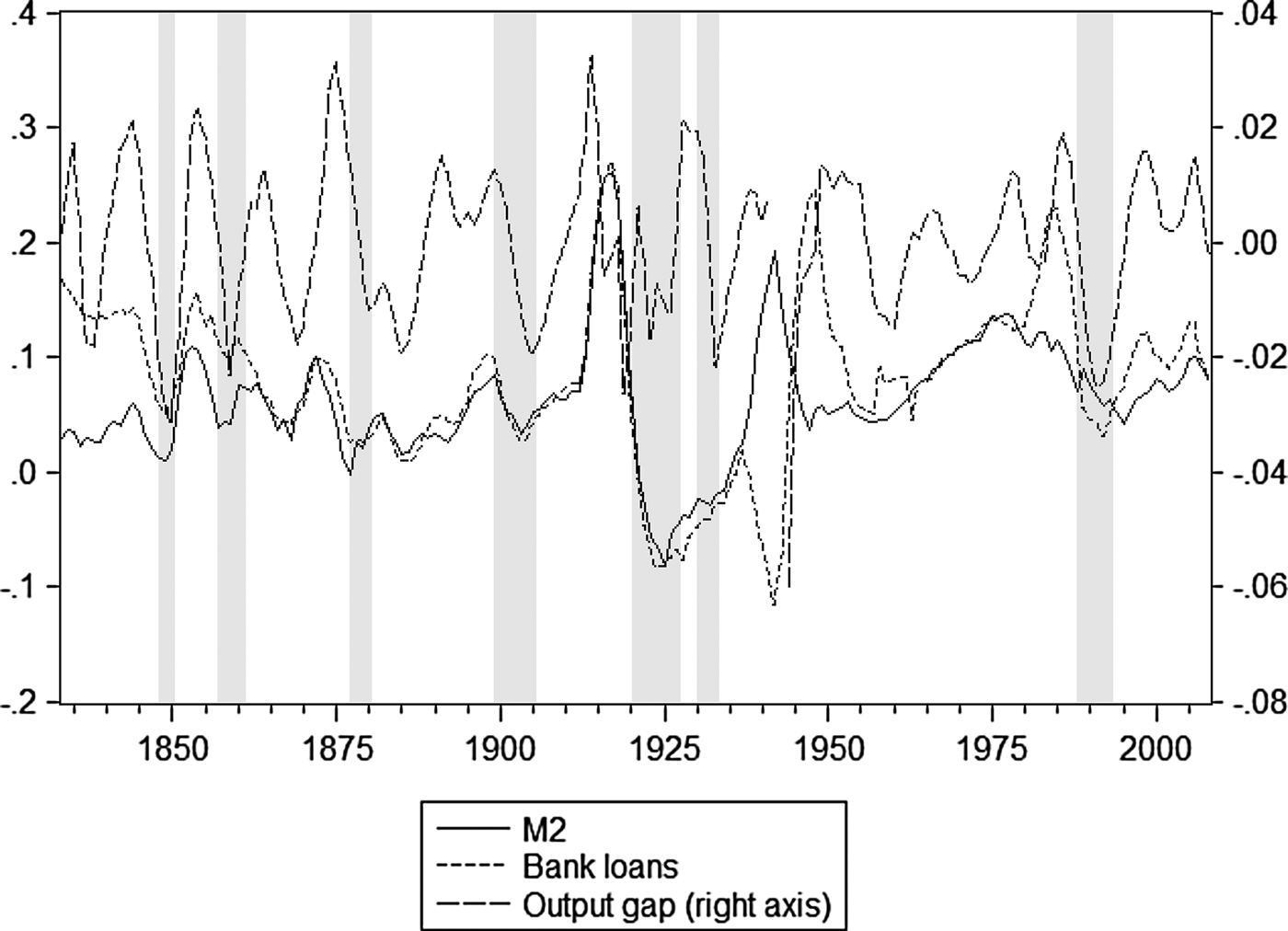
If we calculate the same correlation for the years of financial crises, the correlation coefficient is 0.297. Hence, there is a substantially stronger correlation in times of crises than over the whole time span. We do not attempt to answer the question about the exact nature of this relationship. However, according to Figure 1, there seems to be a mixed relationship between the financial economy and the real economy. One may experience a financial crisis without any significant effect on the real economy.
Output gaps and relative first-order differentials of money stock (M2) and bank loans (BL) for Norway. Five-year symmetric moving averages
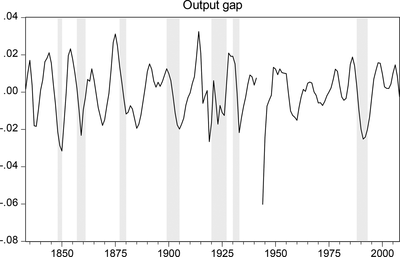
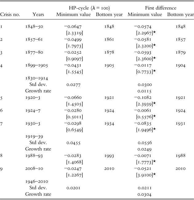
A more relevant parameter would be the output gap. Figure 2 shows that output tends to contract considerably during or shortly after financial markets start to melt down. We find such a relationship for all of our major financial crises, except for the par crisis in the mid 1920s, when output contraction was modest. However, this output contraction must be considered in connection with the huge contraction in the early 1920s, which made the potential decrease lower during the crisis that followed just afterward.
Output gaps for Norway. Five-year symmetric moving averages
The coexistence of financial crises and output contraction is summed up in Table 3. It reports negative output gaps and accumulated drops in GDP during or just after busts. Huge and lasting shocks ending in substantial financial busts historically result in contractions in the real economy.
Contractions in GDP during financial crises
* Standard deviation from the average growth rate
Tables 1 and 2 also report that all the financial crises were associated with drops in manufacturing output, stagnant employment and increased unemployment.
VI
Is there a link between monetary and credit expansion on the one hand and booms and busts on the other hand, as argued by Minsky and Kindleberger?
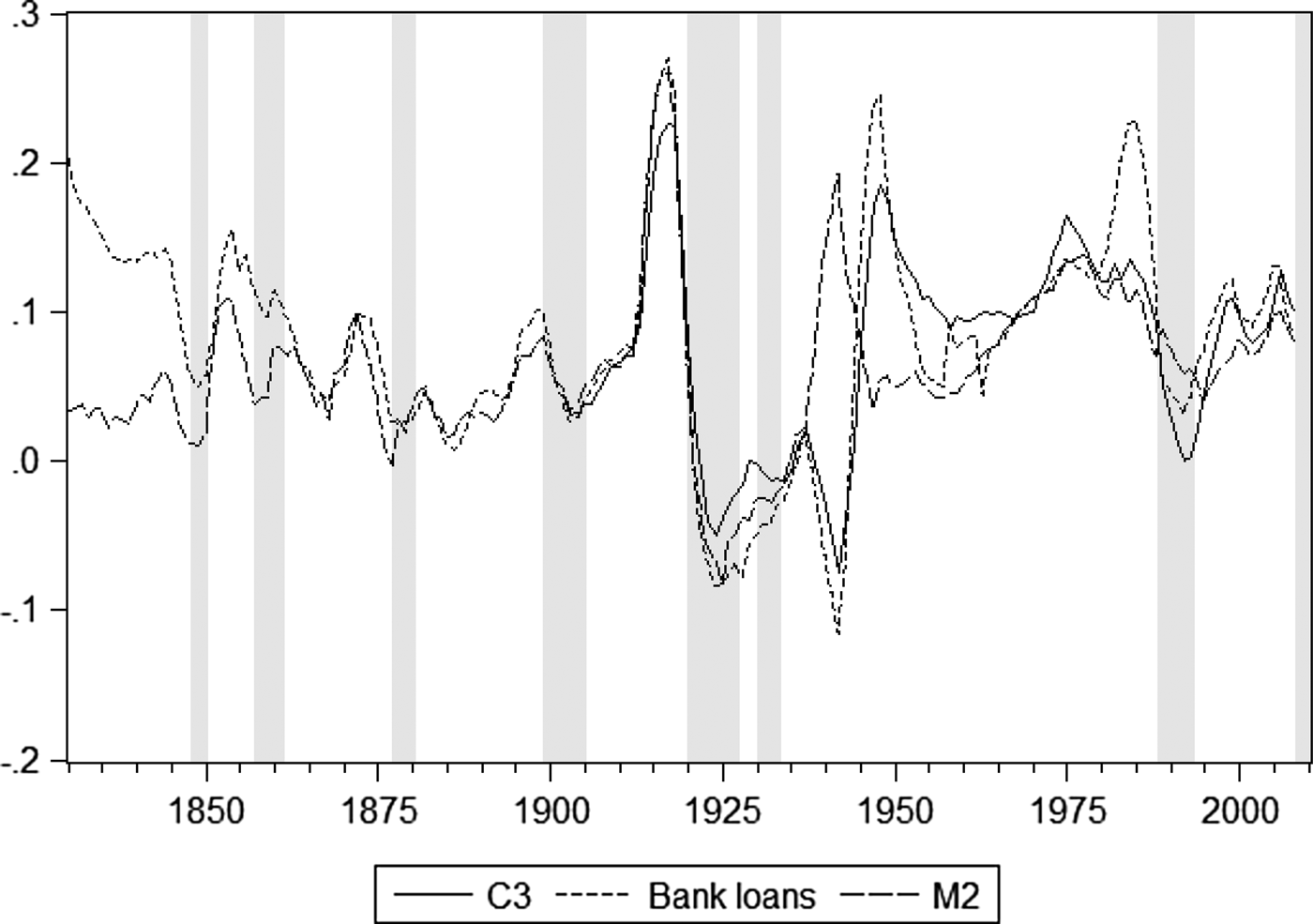
Figure 3 reports relative changes in the money stock (M2), bank loans (BL) and the credit volume (C3), calculated as logs (log t−log t-1). The graphs are presented as five-year symmetric averages. They reveal rapid increases in these parameters prior to all the financial crises that we have data for. Likewise, they show contraction in growth during financial crises. Two exceptions are found. Bank loans did not increase rapidly before the 1848 crisis. An important reason for this result is that the first Norwegian commercial bank was not founded until that year.
Relative first-order differentials of money stock (M2), bank loans (BL) and credits (C3) for Norway. Five-year symmetric moving averages
As for the Great Depression of the 1930s, we find neither significant increase in money and credit volumes prior to the crisis nor contraction during the crisis. This might be explained by fact that a financial boom occurred in the US and France owing to a huge increase in money and credit volumes, which was followed by a contraction in these variables during the crisis. Thus, this crisis was an international liquidity-driven boom–bust cycle affecting the Norwegian economy via the foreign sector (Eichengreen Reference Eichengreen1990, pp. 24–82). In addition, active central bank policy to aid struggling banks and rapid abandonment of gold redemption in September 1931 maintained liquidity in the domestic economy (Øksendal Reference Øksendal2007).
Our empirical findings are also consistent with those of Tornell and Westermann (Reference Tornell and Westermann2005), who conclude that boom–bust cycles follow financial liberalization.
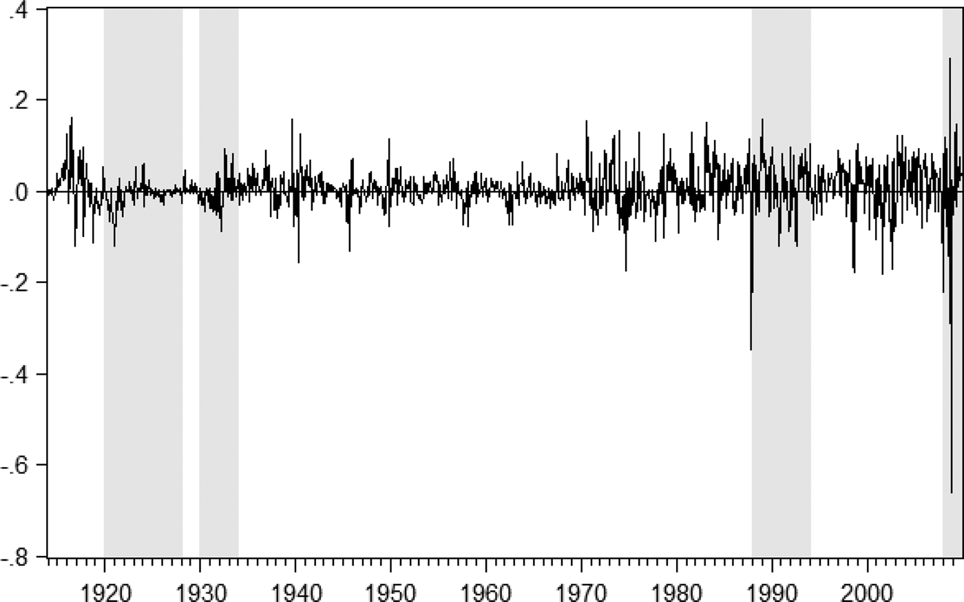
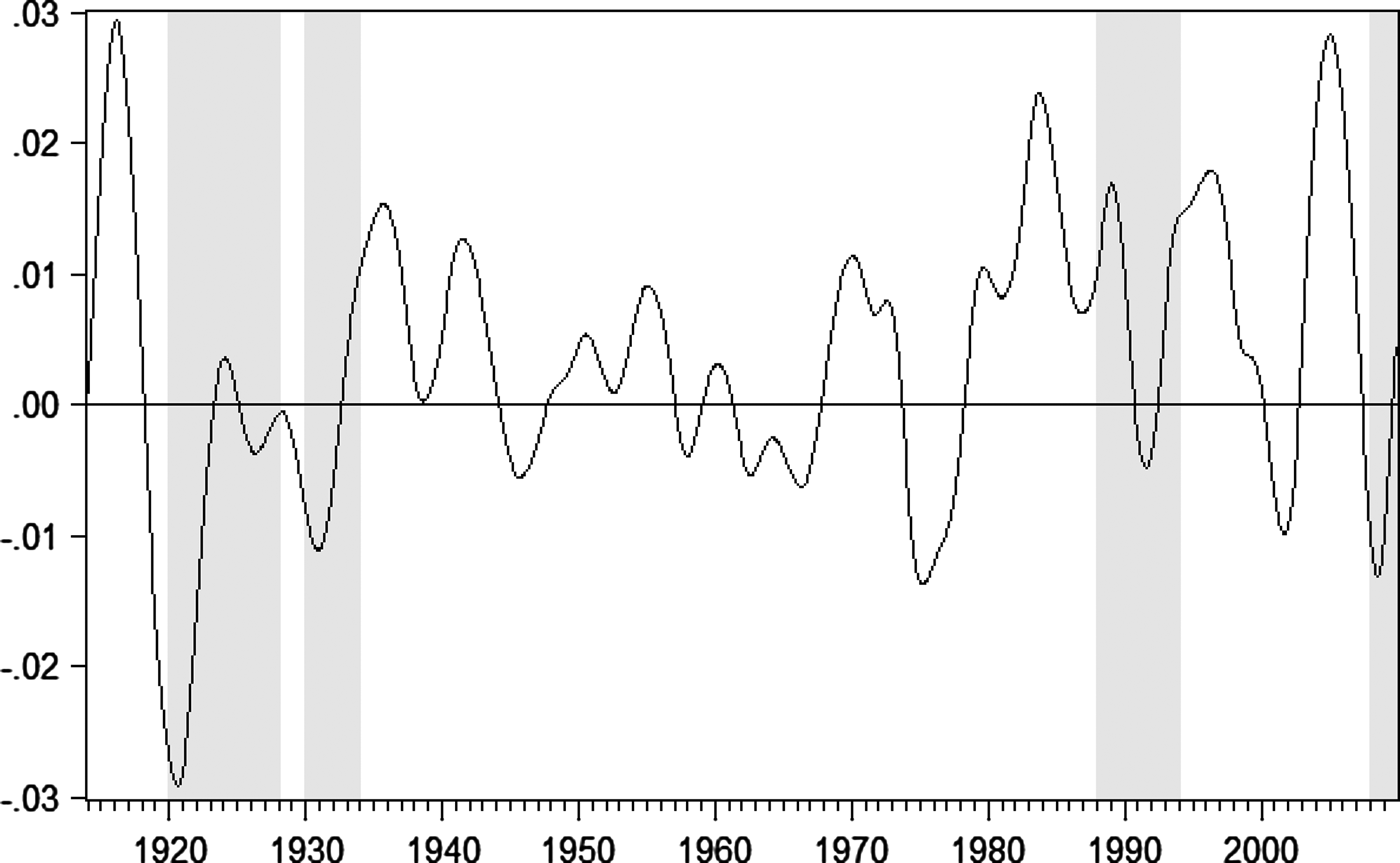
Figure 4 plots monthly changes in the Oslo Stock Exchange main index. To make trends clearer, we HP-filter the data with the standard λ value of 14,400 (Figure 5). By using this smoothing parameter, we clearly trace the boom of stock prices during the credit and money expansion from 1914 onwards. Thereafter, we map the largest stock market crash ever recorded in Norway, which occurred in August 1918.
Oslo Stock Exchange main index. First differentials (logs) of monthly data
HP-filtered Oslo Stock Exchange main index. First differentials (logs) of monthly data, λ = 14,400
We find significant growth in stock prices along with considerable credit and money expansion in the 1980s before a new double crash in September to December 1987, as well as from July 1990 to September 1992 and before the 2008 crash.
The evidence on the change in public debt is mixed (Tables 1 and 2). However, there is a tendency for public debt to increase toward the end of a crisis period.
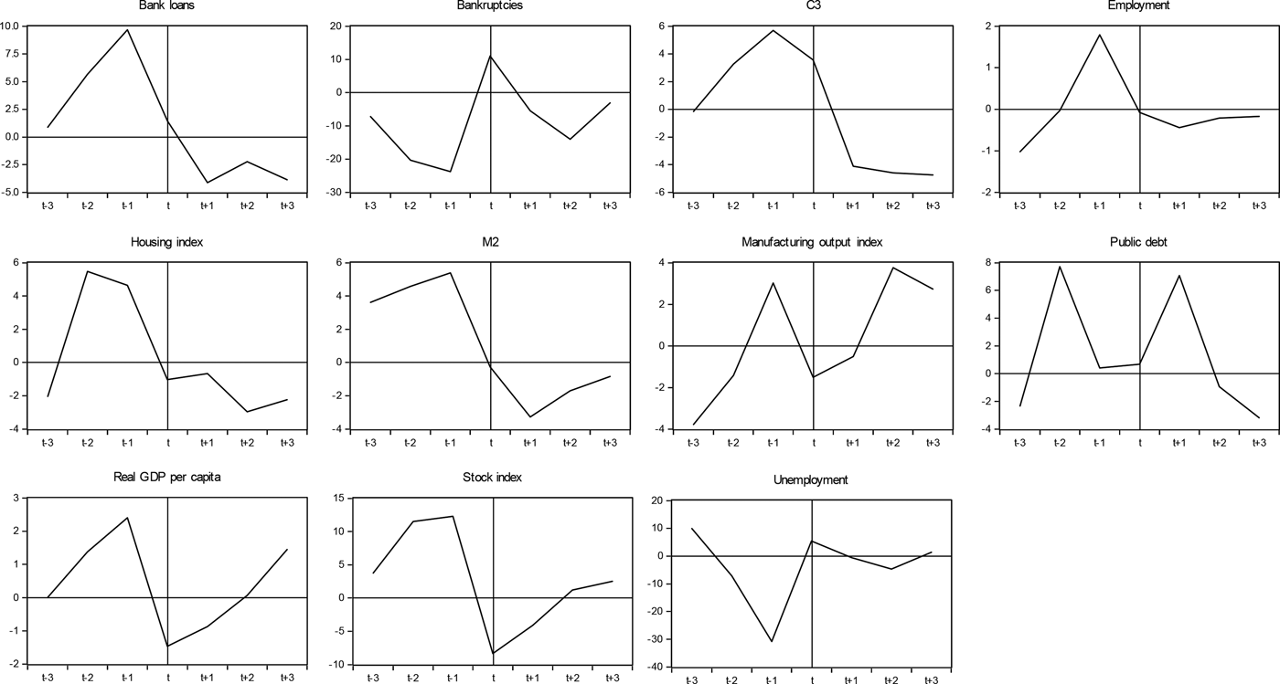
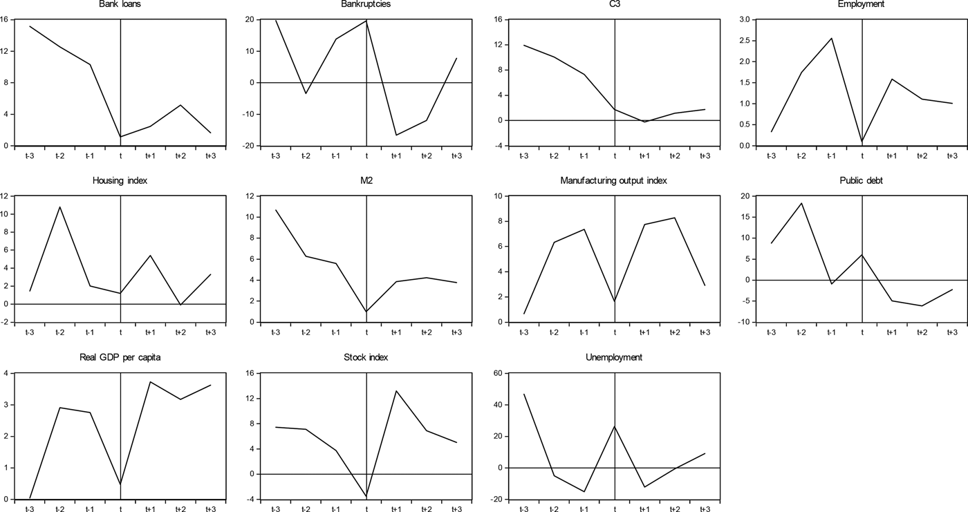
To visualize the pattern, Figures 6 and 7 show a time-window approach. For each crisis, we define year t as the average of the crisis year, as outlined earlier in this article. In addition, we look at the three years before and after the crisis. Then we take the average over all nine crises.
Economic variables and financial crises. Percentage deviation from trend
Economic variables and financial crises. Percentage of annual change
As shown in Figure 6, the economy is generally in a boom before a crisis. It should be noted that the figures summarize nine different crises over a time span of almost two centuries. Nevertheless, the overall pattern seems to be consistent with existing knowledge of financial crises.
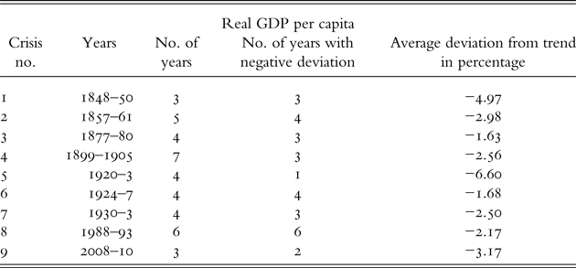
Table 4 presents numbers of the cost of financial crises measured as loss in real GDP per capita. From the table, we see that the crisis in the beginning of the 1920s had the largest drop in output.
Cost of crises in percentage of GDP
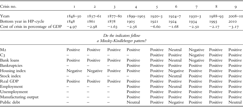
Table 5 sums up the pattern of the indicators that we apply. For each variable, we qualitatively assess whether the variables follow a Minsky–Kindleberger pattern, i.e. an increase during the boom and then a decrease. Unemployment and bankruptcies are expected to have the opposite pattern. According to the table, the majority of the indicators follow such a pattern.
Do the crises follow a Minsky–Kindleberger pattern?
VII
Minsky and Kindleberger argue that monetary expansion through credit liberalization and increased loaning activity cause financial booms and busts with spillover effects on the real economy. In this article, we analyze whether these findings also apply to Norway. First, we identify financial busts on the basis of existing research and financial key indicators. We find nine major financial crises. Thereafter, we seek to determine whether financial crises had spillovers to the real economy. We find such a relationship for most crises. Finally, the article seeks to find out whether developments in money and credit stocks coincide with booms and busts. Our findings confirm that money and credit expansion seem to disturb financial stability and overfuel booms, ending in financial crises. A next step in investigating these relationships could be to apply econometrics, by using cointegration and determining whether any Granger causality exists among the variables. This we leave for future research.
Data Appendix
Descriptive statistics
Plot of the variables