1. Introduction
Non-ideal compressible fluid dynamics (NICFD) is a branch of gas dynamics devoted to the study of flows near the liquid–vapour saturation curve, the critical point, and in supercritical conditions. Their behaviour differs significantly from that observed in typical dilute-gas thermodynamic states, since the ideal-gas law fails to describe the thermodynamics involved (Guardone et al. Reference Guardone, Colonna, Pini and Spinelli2024). Here, the term dilute refers to thermodynamic states characterised by pressures well below the critical pressure, in which the ideal-gas law accurately models the thermodynamic behaviour of the fluid, in contrast with dense vapours. The compressibility factor
 \begin{equation} Z=\frac {P}{\rho R T}, \end{equation}
where
 $P$
is pressure,
 $\rho$
is density,
 $R$
is the gas constant, and
 $T$
is temperature, is commonly used as a measure of non-ideality and to identify non-ideal thermodynamic effects. For ideal gases, the relation
 $P = \rho R T$
holds, namely
 $Z \equiv 1$
. Any deviation of
 $Z$
from unity reflects a quantitative departure from the ideal-gas behaviour. Beyond these quantitative discrepancies, more complex qualitative differences, termed non-ideal gas dynamic effects, are also possibly observed depending on the value of the parameter
 \begin{equation} \varGamma = 1+ \frac {\rho }{c} \left (\frac {\partial c}{\partial \rho } \right )_s \!, \end{equation}
referred to as the fundamental derivative of gas dynamics (Thompson Reference Thompson1971). Here,
 $c=\sqrt { ( \partial P/ \partial \rho )_s}$
is the speed of sound, and
 $s$
is the specific entropy per unit mass. Different gas dynamic regimes can be defined based on the value of
 $\varGamma$
(Guardone et al. Reference Guardone, Colonna, Pini and Spinelli2024). Flows developing through thermodynamic states featuring
 $\varGamma \gt 1$
qualitatively exhibit the gas dynamics of ideal gases, and only non-ideal thermodynamic effects may arise. In contrast, if the flow evolves through states with
 $\varGamma \lt 1$
, i.e. in the so-called non-ideal classical regime, then qualitatively different non-ideal gas dynamic effects are possibly observed. Noteworthy examples include the Mach number decrease in steady supersonic expansions (see e.g. Cramer & Best Reference Cramer and Best1991; Cramer & Fry Reference Cramer and Fry1993; Romei et al. Reference Romei, Vimercati, Persico and Guardone2020), and the increase of the Mach number across oblique shock waves (Vimercati, Gori & Guardone Reference Vimercati, Gori and Guardone2018). In the non-classical regime, negative values of
 $\varGamma$
lead to smooth isentropic compressions, while rarefactions coalesce over time to form shock waves (see e.g. Thompson & Lambrakis Reference Thompson and Lambrakis1973; Menikoff & Plohr Reference Menikoff and Plohr1989). State-of-the-art thermodynamic models (Colonna et al. Reference Colonna, Guardone, Nannan and van der Stelt2009; Thol et al. Reference Thol, Dubberke, Rutkai, Windmann, Köster, Span and Vrabec2016) predict values
 $\varGamma \lt 1$
in the vapour phase region close to saturation for fluids with high molecular complexity. Fluids with even higher molecular complexity are expected to allow for
 $\varGamma \lt 0$
states in the vapour phase, and are referred to as Bethe–Zel’dovich–Thompson (BZT) fluids (Bethe Reference Bethe1942; Zel’dovich Reference Zel’dovich1946; Thompson Reference Thompson1971).
Flows occurring in the non-ideal compressible flow regime are of great interest due to their occurrence in several engineering applications, including rocket propulsion (Bellan Reference Bellan2020), heat pumps (Zamfirescu & Dincer Reference Zamfirescu and Dincer2009), refrigeration and chemical processes (Debenedetti et al. Reference Debenedetti, Tom, Kwauk and Yeo1993; Maincent & Williams Reference Maincent and Williams2016). In power generation, non-ideal flows occur in supercritical carbon dioxide (sCO
 $_2$
) power cycles (see e.g. Angelino Reference Angelino1968; White et al. Reference White, Bianchi, Chai, Tassou and Sayma2021) and are particularly important in organic Rankine cycles (ORCs), which exploit molecularly complex organic compounds instead of steam as working fluid (Colonna et al. Reference Colonna, Casati, Trapp, Mathijssen, Larjola, Turunen-Saaresti and Uusitalo2015; Macchi & Astolfi Reference Macchi and Astolfi2016). Rankine cycles operating with organic fluids are particularly suitable for the exploitation of low to medium temperature sources, such as waste heat from industrial processes, solar radiation and geothermal reservoirs. Due to high molecular complexity and non-ideal effects, the speed of sound in these flows is low compared to that of other simple gases, and expansion processes in turbine stators likely involve supersonic flows even if modest flow velocities are attained (see Colonna et al. Reference Colonna, Harinck, Rebay and Guardone2008; Talluri & Lombardi Reference Talluri and Lombardi2017). In this respect, an accurate treatment of supersonic compressions and expansions in the non-ideal regime is crucial for a proper design of turbomachinery devices.
Non-ideal thermodynamic effects also play a significant role in boundary-layer stability. In adiabatic flows of supercritical and subcritical molecularly complex fluids, stability is enhanced due to the large value of the specific heat, which limits the temperature rise caused by viscous dissipation and thus reduces the boundary-layer growth (Gloerfelt et al. Reference Gloerfelt, Robinet, Sciacovelli, Cinnella and Grasso2020). By contrast, near the liquid–vapour critical point or across the Widom line, strong gradients of thermodynamic and transport properties can promote the onset of instabilities (Ren & Kloker Reference Ren and Kloker2022; Ren et al. Reference Ren, Wu, Mao, Wang and Kloker2025).
Despite the numerous applications in a wide variety of technical fields and the continuous improvement of computational fluid dynamics (CFD) solvers (see e.g. Vitale et al. Reference Vitale, Gori, Pini, Guardone, Economon, Palacios, Alonso and Colonna2015; Sciacovelli et al. Reference Sciacovelli, Cinnella, Content and Grasso2016, Reference Sciacovelli, Cinnella and Gloerfelt2017; Giauque, Corre & Vadrot Reference Giauque, Corre and Vadrot2020), detailed experimental data characterising non-ideal flows are still limited in the open literature, due to the challenging operating conditions and measurement procedures (Guardone et al. Reference Guardone, Colonna, Pini and Spinelli2024). Nonetheless, the number of dedicated facilities is rapidly increasing (see e.g. Spinelli et al. Reference Spinelli, Pini, Dossena, Gaetani and Casella2013; Head et al. Reference Head, De Servi, Casati, Pini and Colonna2016; Reinker et al. Reference Reinker, Kenig, Passmann and aus der Wiesche2017; Beltrame et al. Reference Beltrame, Head, De Servi, Pini, Schrijer and Colonna2021; Petruccelli et al. Reference Petruccelli, Uusitalo, Grönman, Turunen-Saaresti and Zocca2021; Chandrasekaran et al. Reference Chandrasekaran, Michelis, Mercier and Colonna2022), and several measurement techniques are being tested and developed (see Conti et al. Reference Conti, Fusetti, Spinelli, Gaetani and Guardone2022b ; Michelis et al. Reference Michelis, Head, Majer, Colonna and De Servi2024).
The present work focuses on the measurement of the Prandtl–Meyer function in the non-ideal compressible flow regime. For a steady, isentropic, supersonic flow, the Prandtl–Meyer function
 $\nu$
is defined by the differential relation (Thompson Reference Thompson1988)
 \begin{equation} \textrm{d}\nu = \frac {\sqrt {M^2-1}}{1+ \left ( \varGamma -1 \right ) M^2} \frac {\textrm{d}M}{M} , \end{equation}
where
 $M = u/c$
is the Mach number, with
 $u$
the fluid velocity. For a polytropic ideal gas (PIG), the fundamental derivative is constant,
 $\varGamma = (\gamma +1)/2 \gt 1$
, where
 $\gamma \gt 1$
is the specific heat ratio, and (1.3) can be integrated analytically, providing the expression
 \begin{equation} \nu _{ {PIG}} (M) = \sqrt {\frac {\gamma +1}{\gamma -1}} \arctan \sqrt {\frac {\gamma -1}{\gamma +1} \left (M^2-1\right )} - \arctan \sqrt {M^2-1}. \end{equation}
The quantity
 $\nu$
formally represents the flow deflection angle required to reach a specific Mach number
 $M$
from uniform sonic flow conditions. For a PIG, the post-expansion Mach number depends only on the upstream Mach number and the deflection angle, provided that the fluid – and thus the value of
 $\gamma$
– is given.
For non-ideal flows, Cramer & Crickenberger (Reference Cramer and Crickenberger1992) computed numerically the Prandtl–Meyer function by solving the equations
 \begin{align} \frac {\textrm{d}\nu }{\textrm{d} \rho } &= - \frac {\sqrt {M^2 -1}}{\rho M^2}, \end{align}
 \begin{align} \frac {\textrm{d} M}{\textrm{d} \rho } &= \frac {M}{\rho } \left (1 - \varGamma - \frac {1}{M^2} \right )\!, \end{align}
 \begin{align} \frac {\textrm{d} T}{\textrm{d} \rho } &= \frac {T}{\rho c_v} \left ( \frac {\partial P}{\partial T} \right )_\rho \!, \end{align}
where
 $c_v$
is the constant-volume specific heat. If fluid thermodynamic properties are non-ideal, then the flow evolution strongly depends on the upstream state, or equivalently, on the stagnation properties (Wheeler & Ong Reference Wheeler and Ong2013). The non-dimensional parameter
 $J = 1 - \varGamma - 1/M^2$
, first introduced by Cramer & Best (Reference Cramer and Best1991), quantifies the Mach number variation with the density in isentropic processes. According to (1.5b
), for values of
 $J\lt 0$
, the Mach number increases along isentropic expansions, as in the case of ideal gases. On the contrary, positive values of
 $J$
are associated with a decrease of the Mach number for decreasing density. The latter condition is only possible in the non-ideal gas dynamic regime, for thermodynamic conditions featuring
 $\varGamma \lt 1$
, and at sufficiently large Mach numbers. For BZT fluids, non-monotonic Mach number evolution is also possible in the subsonic regime when
 $\varGamma \lt 0$
.
Figure 1 shows the evolution of the Mach number across Prandtl–Meyer expansions for different thermodynamic conditions, identified by the value of the compressibility factor evaluated at total conditions
 $Z_{\textit{t}}$
. The fluid considered is the high molecular complexity siloxane MM (hexamethyldisiloxane,
 $\textrm{C}_{6}\textrm{H}_{18}\textrm{OSi}_{2}$
), and thermodynamics is modelled through the state-of-the-art Helmholtz-form Span–Wagner equation of state (Span & Wagner Reference Span and Wagner2003), defined by means of 18 parameters determined from measurements and reported in Thol et al. (Reference Thol, Dubberke, Rutkai, Windmann, Köster, Span and Vrabec2016). The ideal-gas solution is also reported as reference. At mildly non-ideal conditions, i.e. for
 $Z_{\textit{t}}\gt 0.60$
, non-ideal thermodynamic effects arise, as only quantitative deviation from ideal-gas behaviour is observed, and this deviation increases with growing non-ideality. At these mildly non-ideal conditions, the relative difference between the Mach number computed using the Span–Wagner equation of state and the improved Peng–Robinson–Stryjek–Vera (iPRSV) (Van der Stelt, Nannan & Colonna Reference Van der Stelt, Nannan and Colonna2012) equation of state is within 1 %. At stronger non-ideal conditions, non-ideal gas dynamic effects exhibit as qualitatively different flow evolutions. In particular, for thermodynamic states close enough to saturation, as in the case of the curve at
 $Z_{\textit{t}} = 0.40$
, the fundamental derivative
 $\varGamma$
is low enough to make
 $J$
positive, resulting in the Mach number reduction across the expansion.
Variation of the Mach number
 $M$
with the flow deflection angle
 $\theta$
across Prandtl–Meyer expansions in fluid MM under different thermodynamic conditions, assuming sonic upstream flow.

In the present work, experimental measurements of the Prandtl–Meyer function in non-ideal conditions are presented. Planar supersonic expansions generated at sharp convex corners, namely Prandtl–Meyer expansions, are investigated, since flow entropy is typically preserved. Nonetheless, the presented results have broader applicability, since the Prandtl–Meyer function also characterises compression processes, provided that isentropic conditions are satisfied. Experiments are carried out within the TROVA supersonic wind tunnel of Politecnico di Milano (see Spinelli et al. Reference Spinelli, Pini, Dossena, Gaetani and Casella2013, Reference Spinelli, Cozzi, Cammi, Zocca, Gaetani, Dossena and Guardone2017), by using the organic compound MM, commonly employed in medium/high-temperature ORCs. Non-ideal thermodynamic effects are presented as quantitative variations in the flow evolution for different stagnation thermodynamic conditions (see figure 1). However, limitations related to plant operability and thermal stability issues precluded the observation of non-ideal gas dynamic effects. Nonetheless, the presented results expand the currently available measurements in the NICFD field, and provide additional data for the validation of numerical codes.
The structure of the present work is as follows. The experimental set-up and the geometry are described in § 2. Section 3 presents the operating thermodynamic conditions of the experimental tests. Results are discussed in § 4, including schlieren visualisations and pressure and Mach number measurements. Non-ideal effects in the investigated flow are highlighted, and measurements of the Prandtl–Meyer function are presented. Concluding remarks are provided in § 5.
2. Experimental facility and set-up
The experimental campaign reported in the present work was carried out in the Test Rig for Organic VApours (TROVA) of the Laboratory of Compressible-fluid dynamics for Renewable Energy Applications (CREALab) of Politecnico di Milano. The TROVA is a supersonic blow-down wind tunnel designed to characterise non-ideal flows across a wide variety of organic fluids and thermodynamic conditions (see Spinelli et al. Reference Spinelli, Pini, Dossena, Gaetani and Casella2013, Reference Spinelli, Cozzi, Cammi, Zocca, Gaetani, Dossena and Guardone2017). The working fluids are liquid at room temperature. A high-pressure vessel (HPV) is charged with the amount of fluid required to reach, after being isochorically heated and vapourised, the desired pressure and temperature setpoint. The flow is then discharged from the HPV to a previously vacuumised low-pressure vessel (LPV), by passing through a settling chamber and expanding in a planar test section, which can accommodate different geometries. A more detailed description of the facility and its components is provided in Appendix A. Due to the blow-down nature of the TROVA, the operating pressure and temperature decrease in time during the test, and different thermodynamic conditions, namely different levels of non-ideality, are observed within a single test. Previous campaigns carried out in the TROVA allowed for an extensive experimental characterisation of non-ideal compressible flows, including non-ideal effects in isentropic expanding flows (Spinelli et al. Reference Spinelli, Cammi, Gallarini, Zocca, Cozzi, Gaetani, Dossena and Guardone2018; Zocca, Gajoni & Guardone Reference Zocca, Gajoni and Guardone2025) and in oblique and normal shock waves (Zocca et al. Reference Zocca, Guardone, Cammi, Cozzi and Spinelli2019; Conti et al. Reference Conti, Fusetti, Spinelli and Guardone2022a ).
In the experiments presented here, the plant is operated using siloxane compound MM. The test section accommodates a converging–diverging nozzle that delivers a uniform supersonic flow. The flow is then deflected three times by means of sudden variations of the slope of the wall to generate three Prandtl–Meyer expansions. A brief description of the test rig and the instrumentation is provided for completeness in § 2.1, while § 2.2 focuses on the geometric configuration.
2.1. Test rig and instrumentation
Figure 2 shows the test section in the present experimental campaign. Two planar contoured profiles are mounted on a mirror-polished backplate; see figure 2(a). The profiles can be easily replaced to simulate different geometry configurations. Opposite to the backplate, a quartz window is mounted to allow optical access to the flow. Piezo-resistive pressure transducers, wall mounted at pressure taps on the backplate (see figure 2
b), provide static pressure measurements at discrete locations along the centreline of the test section. Similarly, the stagnation pressure
 $P_{\textit{t}}$
is measured in the settling chamber upstream of the test section, where the flow velocity is approximately 1 m s−1. Under this condition, static and total pressure coincide, allowing the total pressure to be accurately determined using a wall pressure tap. The stagnation temperature
 $T_{\textit{t}}$
is measured by two thermocouples positioned at the symmetry axis of the settling chamber. The total conditions experienced by the test section are measured immediately upstream, in the settling chamber. Due to the variation of the operating conditions over time, and to non-quantifiable pressure losses occurring in the valves between the HPV and the test section, the measurements performed in the settling chamber are essential for evaluating the degree of flow non-ideality at each instant of the test. Expanded uncertainties (Gaussian, 95 % confidence level) for pressure sensors are of the order of
 $0.07\,\%$
of the full scale, resulting in approximately 0.04 bar for total pressure, and approximately 0.015 bar for static pressure, for the transducers used in this campaign. Expanded uncertainty for thermocouples is approximately
 $1\,^\circ\text{C}$
. More details about pressure and temperature measurements can be found in Cammi (Reference Cammi2019).
Test section mounted during the present experimental campaign. (a) Mirror-polished backplate with contoured profiles (flow from left to right). (b) Back closure of the test section and view of the flush-mounted pressure transducers.

A double-passage parallel-light schlieren system, equipped with a CMOS camera, complements pressure and temperature measurements providing flow visualisations. The schlieren knife is rotated so that lighter grey levels correspond to negative density gradients in the flow direction (expansions), and darker grey levels to positive ones (compressions). Details on the schlieren set-up of the TROVA are available in Cozzi et al. (Reference Cozzi, Spinelli, Carmine, Cheli, Zocca and Guardone2015).
Schlieren visualisations are a particularly powerful tool in the field of non-ideal compressible flows. Due to the large compressibility of the fluids involved, even a small density gradient results in a large gradient of the fluid refractive index (see Conti et al. Reference Conti, Spinelli, Cammi, Zocca, Cozzi and Guardone2017). This provides a clear visualisation of Mach waves originating from the rough contoured profiles of the test section, in the supersonic portion of the flow domain. The roughness of solid walls introduces small perturbations in the flow, which propagate through the flowfield as Mach waves, and according to the theory of characteristics for two-dimensional supersonic flows, they locally align with the characteristic directions; see Thompson (Reference Thompson1988). Perturbations originating at the lower wall propagate along
 $C^+$
characteristic lines, while those generated at the upper wall propagate along
 $C^-$
lines. Characteristic lines belonging to different families intersect, forming a characteristic net. Therefore, besides providing a visualisation of the entire flowfield, schlieren images allow direct flow measurements. Guardone et al. (Reference Guardone, Zocca, Gajoni, Mondonico and Conti2025) suggested using the slopes of two intersecting Mach lines of different families,
 $\alpha ^+$
and
 $\alpha ^-$
, to compute the Mach angle as
 $\mu = (\alpha ^+ - \alpha ^-)/2$
and the flow direction as
 $\theta = (\alpha ^+ + \alpha ^-)/2$
. The local Mach number is then retrieved from the Mach angle as
 $M = 1/ \sin \mu$
. The expanded uncertainty of the detected line slope is estimated based on Mach line thickness and image resolution. The expanded uncertainty (Gaussian, 95 % confidence level) of the local Mach number is then obtained through direct computation as
 $U_M = M \sqrt {M^2-1}\,U_{\mu }$
, where
 $U_{\mu }$
is the expanded uncertainty of the Mach angle. Note that the uncertainty of Mach number measurements
 $U_M$
increases proportionally to
 $M^2$
, resulting in larger uncertainties for increasing Mach numbers. The reader is referred to Cammi et al. (Reference Cammi, Spinelli, Cozzi and Guardone2021) and Guardone et al. (Reference Guardone, Zocca, Gajoni, Mondonico and Conti2025) for an exhaustive description of the method.
2.2. Test section design
The geometry of the test section employed in the present experimental campaign is shown in figure 3. Due to physical space constraints, two similar geometries, each incorporating three corners, are used to cover the entire range of deflection angles for which the Prandtl–Meyer expansion is observed. Geometry
 $\mathcal{A}$
(figure 3
a) generates Prandtl–Meyer expansions corresponding to flow deflections of 10
 $^\circ$
, 20
 $^\circ$
and 30
 $^\circ$
, whereas geometry
 $\mathcal{B}$
(figure 3
b) provides flow deflections of 5
 $^\circ$
, 15
 $^\circ$
and 25
 $^\circ$
. By combining the results from the two geometries, measurements are available for flow deflections in discrete 5
 $^\circ$
increments up to 30
 $^\circ$
.
Test section geometry. (a) Geometry
 $\mathcal{A}$
generates Prandtl–Meyer expansions through flow deflections of 10
 $^\circ$
, 20
 $^\circ$
and 30
 $^\circ$
. (b) Geometry
 $\mathcal{B}$
provides flow deflections of 5
 $^\circ$
, 15
 $^\circ$
and 25
 $^\circ$
. Fluid flows from left to right. Black dots represent pressure taps, while the grey rectangle identifies the optically accessible region. Expansion fans at design conditions are reported as blue shaded regions.

The flow is accelerated in the test section to the desired supersonic conditions through a converging–diverging geometry (region ACC′A′ in the figure), where BB′ is the geometrical throat. The throat region at the upper wall is made of a circular arc with radius
 $5H$
, where
 $H = 25$
mm is the throat height, i.e. the length of BB′. The upper profile of the supersonic diverging section BC is designed by means of the computational tool NIMOC (Zocca, Gajoni & Guardone Reference Zocca, Gajoni and Guardone2023), which implements the method of characteristics for non-ideal supersonic nozzle flows. Thermodynamics is modelled through the open-source thermodynamic library CoolProp (Bell et al. Reference Bell, Wronski, Quoilin and Lemort2014), using the Span–Wagner equation of state with parameters defined by Thol et al. (Reference Thol, Dubberke, Rutkai, Windmann, Köster, Span and Vrabec2016). The bottom part of the divergent (profile B′C′) is a straight line. For both geometries
 $\mathcal{A}$
and
 $\mathcal{B}$
, the divergent part is designed to discharge at section CC′ a uniform parallel flow of fluid MM with total pressure
 $P_{\textit{t}} = 15.7$
bar, total temperature
 $T_{\textit{t}} = 239$
 $^\circ$
C, and outlet Mach number
 $ M = 1.25$
. The divergent section BCC′B′ is rotated by an angle of 17.5
 $^\circ$
with respect to the horizontal direction to bring the lower wall, where the expansions are generated, closer to the pressure taps, which lie on the test section centreline. The distance between the wall and the taps is sufficient to avoid measurement interference due to interaction with the thin boundary layer. Pressure measurements are thus expected to characterise a pure Prandtl–Meyer expansion. The convergent is designed by smoothly matching the throat region with the inlet section AA′ using third-degree polynomials. The region downstream of section CC′ is designed to generate three expansion fans. The lower profile C′D′ is made of a broken line, which induces three sudden flow deflections. In geometry
 $\mathcal{A}$
, the three sharp corners generate a flow deflection of 10
 $^\circ$
, 20
 $^\circ$
and 30
 $^\circ$
with respect to the flow direction at section CC′. For geometry
 $\mathcal{B}$
, the flow deflections are of 5
 $^\circ$
, 15
 $^\circ$
and 25
 $^\circ$
. Expansion fans at design conditions are reported in figure 3 as blue shaded regions. The small region between section CC′ and the first fan has constant section, therefore the flow remains uniform under design conditions. This allows for easier measurement of the flow upstream of the expansion through both pressure taps and schlieren images. The upper profile CD is designed to cancel the expansion waves generated at the lower wall, avoiding their reflection.
At design conditions, the divergent profile yields uniform supersonic flow conditions, hence region CDD′C′ is a simple-wave region, meaning that characteristic lines belonging to at least one of the two families are straight, and fluid properties are constant along these straight characteristics (Thompson Reference Thompson1988). In particular, the regions between the fans feature uniform flow conditions. This allows for the investigation of canonical Prandtl–Meyer expansions, which are in general typical features of external flows. The location of the fans with respect to pressure taps is carefully studied to provide one direct pressure measurement for each of the uniform regions.
The geometry contours are designed for the specific thermodynamic conditions reported above and without accounting for the presence of the boundary layer. In the actual experiment, the operating conditions change over time, and in addition a thin boundary layer is inevitably present. Consequently, the boundary layer and the dependence of non-ideal flows on the stagnation conditions lead to the geometry operating under conditions that are slightly different from the design ones. As a result, the flow discharged from the divergent section is not perfectly uniform and exhibits a Mach number slightly deviating from the design value. Nonetheless, test conditions are chosen so that these non-uniformities induce a negligible effect on the flow downstream of section CC′. Deviations from design conditions are considered sufficiently small not to affect the investigation of Prandtl–Meyer expansions. This was verified through schlieren measurements (see § 4.2) and CFD simulations. The position of the fans also slightly changes during the test due to non-ideal effects. Nonetheless, pressure taps always remain within the uniform regions.
Reference CFD simulations, used to verify the proper design of the geometries and their off-design operation, were carried out following the methodology proposed by Gori et al. (Reference Gori, Zocca, Cammi, Spinelli, Congedo and Guardone2020) for the simulation of non-ideal compressible flows. Both inviscid and Reynolds-averaged Navier–Stokes (RANS) simulations were performed, the latter employing the
 $k{-}\omega$
shear stress transport turbulence model. Characteristics-based Riemann boundary conditions (see Vitale et al. Reference Vitale, Gori, Pini, Guardone, Economon, Palacios, Alonso and Colonna2015) are applied at the inflow and outflow boundaries of the computational domain. Horizontal flow direction and total conditions are prescribed at the inlet, whereas a static pressure yielding transition to supersonic flow is set at the outlet. Adiabatic walls are assumed, consistent with the experimental set-up in which the test section is heated to a temperature comparable to that of the flow to avoid fluid condensation. Thermodynamics is modelled through the iPRSV equation of state (see Van der Stelt et al. Reference Van der Stelt, Nannan and Colonna2012), which provides accuracy comparable to that of state-of-the-art equations of state within the examined thermodynamic range, while significantly reducing the computational time.
For both geometries and all the investigated thermodynamic conditions, the Reynolds number
 $Re$
based on the throat height
 $H$
at section BB′ and the boundary-layer displacement thickness
 $\delta$
are computed from the RANS computations. The obtained values range from
 $Re = 13 \boldsymbol{\times }10^6$
and
 $\delta = 0.6$
mm upstream of the first expansion, and
 $Re = 1.5 \boldsymbol{\times }10^6$
and
 $\delta = 1.2$
mm downstream of the last expansion. These results indicate that the boundary layer remains turbulent throughout the entire region of interest. Across each expansion, the Reynolds number decreases due to the strong density reduction, whereas the boundary layer thickens. A slight reduction in
 $Re$
and a corresponding increase in
 $\delta$
are observed as the thermodynamic conditions approach dilute states. A small separation bubble is expected at each corner, followed by rapid reattachment driven by the expansion and subsequent flow acceleration (Grilli, Hickel & Adams Reference Grilli, Hickel and Adams2013), although such features are not captured by the RANS model. The favourable pressure gradient across each expansion suppresses instabilities and reduces the predicted turbulent kinetic energy, consistent with experimental and numerical evidence in the literature (see e.g. Gillis & Johnston Reference Gillis and Johnston1983; Arnette, Samimy & Elliott Reference Arnette, Samimy and Elliott1998; Kim, Samimy & Lee Reference Kim, Samimy and Lee2001). Comparison between inviscid and viscous simulations shows that boundary-layer effects have a negligible impact on the accuracy of the Mach number and pressure profiles in the inviscid core due to the high Reynolds number. For this reason, the theoretical estimates presented in the following assume an inviscid flow.
3. Operating conditions
The batch operating mode of the TROVA is such that at each time instant during the test, a different dataset (including total temperature, total and static pressures, and schlieren frame) is acquired. The HPV emptying process, which lasts approximately 100 s, is significantly slower than the characteristic time of the flow residence in the test section (
 $\sim 1.5$
ms), therefore each dataset is considered as an independent steady-state representation of the flowfield (see Spinelli et al. Reference Spinelli, Pini, Dossena, Gaetani and Casella2013). During the residence time of the flow in the test section, variations of the order of 0.15 % for total pressure and 0.01 % for total temperature occur, well below the measurement uncertainties of the sensors, which are approximately 0.65 % and 0.5 %, respectively. Moreover, no significant unsteadiness is detected by the sensors, acquiring at sampling frequency 1 kHz, further confirming the quasi-steady assumption for the plant operation.
Several tests were run with both geometries to ensure repeatability of the experimental results. Four tests are reported in the present paper, two for each of the geometries. Figure 4 shows, in a pressure–temperature thermodynamic diagram, the evolution of total pressure
 $P_{\textit{t}}$
and total temperature
 $T_{\textit{t}}$
during the tests, directly measured in the settling chamber upstream of the test section. Expanded uncertainties of the total conditions and contours of the compressibility factor
 $Z_{\textit{t}}$
are reported.
Pressure–temperature thermodynamic diagram of siloxane MM with total thermodynamic conditions of the tests. The thick solid line is the saturation curve, and contours of the compressibility factor
 $Z_{\textit{t}}$
are reported. Total test conditions evolve from lower to larger
 $Z_{\textit{t}}$
. The slight deviation of total temperature towards the end of tests
 $\mathcal{A}$
1 and
 $\mathcal{B}$
1 is possibly due to differences in the external temperature in the laboratory. Nonetheless, measured values in the two tests remain within each other’s experimental uncertainties.

Tests are labelled as the name of the geometry, followed by a number. With reference to figure 4, tests
 $\mathcal{A}$
1 and
 $\mathcal{B}$
1 reproduce almost the same total conditions in time, with different geometries. The same is valid for tests
 $\mathcal{A}$
2 and
 $\mathcal{B}$
2. While runs
 $\mathcal{A}$
1 and
 $\mathcal{B}$
1 feature medium pressure and temperature in the HPV at the beginning of the experiment, runs
 $\mathcal{A}$
2 and
 $\mathcal{B}$
2 attain higher conditions, but with comparable compressibility factors
 $Z_{\textit{t}}$
.
The beginning of the tests is characterised by high pressure and temperature (top right region in figure 4). Then following the emptying process of the HPV, both pressure and temperature decrease in time. In consequence, higher non-ideal conditions are observed at the beginning of the test, where the compressibility factor at total conditions
 $Z_{\textit{t}} \lt 0.60$
and non-ideal effects are important. At the end of the test, more dilute thermodynamic conditions are attained, and close-to-ideal conditions are observed (
 $Z_{\textit{t}} \gt 0.90$
).
Throughout the paper, data are classified based on the value of
 $Z_{\textit{t}}$
. The compressibility factor evaluated at total conditions represents a suitable similarity parameter for complex fluids in moderately high non-ideal conditions (Conti, Spinelli & Guardone Reference Conti, Spinelli and Guardone2021). Total thermodynamic conditions of the tests are reported in table 1, for three values of the compressibility factor. The repeatability of experimental data is assessed from repeated tests by comparing measurements at the same value of
 $Z_{\textit{t}}$
, following the procedure described by Spinelli et al. (Reference Spinelli, Cammi, Gallarini, Zocca, Cozzi, Gaetani, Dossena and Guardone2018) and Conti et al. (Reference Conti, Spinelli and Guardone2021).
Total pressure
 $P_{\textit{t}}$
and temperature
 $T_{\textit{t}}$
of the tests with experimental uncertainties (Gaussian, 95 % confidence level) for different values of the compressibility factor at total conditions
 $Z_{\textit{t}}$
.

4. Results and discussion
Measurements are now presented and compared to the Prandtl–Meyer theory. Thanks to the excellent matching of operating conditions between tests performed with different geometries (see table 1), tests
 $\mathcal{A}$
1 and
 $\mathcal{B}$
1 are combined to create a single dataset, referred to as dataset 1. Similarly, tests
 $\mathcal{A}$
2 and
 $\mathcal{B}$
2 are combined to form dataset 2. Tests
 $\mathcal{A}$
1 and
 $\mathcal{B}$
1 are taken as reference and are thoroughly discussed in §§ 4.1 to 4.4. The two datasets are then compared to provide insights into the role of the compressibility factor evaluated at total conditions
 $Z_{\textit{t}}$
.
In each test, static pressure measurements
 $P$
are obtained from pressure taps. Mach number measurements
 $M$
are obtained from the analysis of the acquired schlieren images, following the procedure described in § 2. Schlieren visualisations are acquired at frequency 10 Hz with exposure time 0.87 ms. Instantaneous frames corresponding to the desired operating conditions are selected and post-processed. Measured total thermodynamic conditions
 $P_{\textit{t}}$
and
 $T_{\textit{t}}$
are assumed uniform in the entire flowfield outside the thin boundary layer. Under this hypothesis, both pressure taps and schlieren measurements can independently provide a complete description of the flowfield in terms of thermodynamic state and fluid dynamics variables, as detailed by Guardone et al. (Reference Guardone, Zocca, Gajoni, Mondonico and Conti2025). Total enthalpy and specific entropy are computed from the measured total quantities as
 $h_{\textit{t}} = h(P_{\textit{t}},T_{\textit{t}})$
and
 $s = s(P_{\textit{t}},T_{\textit{t}})$
, respectively, under Span–Wagner thermodynamics, and they are also conserved through the flowfield. The Mach number can thus be obtained from the static pressure measured at pressure taps as
 \begin{equation} M_{\textit{taps}} = \frac {u}{c} = \frac {\sqrt {2\left ( h_{\textit{t}} - h(P_{\textit{taps}}, s) \right )}}{c(P_{\textit{taps}}, s)}, \end{equation}
where specific enthalpy
 $h$
and speed of sound
 $c$
are computed from the measured static pressure
 $P_{\textit{taps}}$
and the entropy
 $s$
. On the other hand, pressure can be retrieved from schlieren measurements as
 $P_{\textit{sch}} = P(h_{\textit{sch}}, s)$
, where the static enthalpy
 $h_{\textit{sch}}$
is found by solving the implicit nonlinear equation
 \begin{equation} h_{\textit{sch}} + \frac {1}{2}M_{\textit{sch}}^2 c^2(h_{\textit{sch}},s) - h_{\textit{t}} = 0. \end{equation}
Independent measurements from pressure taps and schlieren images are therefore compared in terms of both static pressure and Mach number.
Theoretical results are obtained from the integration of (1.5) by fourth-order Runge–Kutta methods, complemented with the Span–Wagner equation of state, where total enthalpy and specific entropy are assumed constant through the integration.
Subsection 4.1 describes the flow layout from schlieren visualisations, while pressure and Mach number measurements are reported in § 4.2. A discussion of non-ideal effects from experimental data is carried out in § 4.3. Finally, in § 4.4, the Prandtl–Meyer function is retrieved from the experimental data.
4.1. Schlieren visualisations
Figure 5 reports schlieren visualisations of the flowfield for the two geometries and different thermodynamic conditions, from tests
 $\mathcal{A}$
1 and
 $\mathcal{B}$
1. Geometry
 $\mathcal{A}$
is shown in figure 5(a,c), while geometry
 $\mathcal{B}$
is shown in figure 5(b,d). Figure 5(a,b) show the flowfield for
 $Z_{\textit{t}} = 0.60$
, namely at dense non-ideal conditions. The schlieren technique clearly shows all compressible flow features, as both Mach lines and expansion fans are very pronounced. Note that expansion fans appear as black regions, as observed by Conti et al. (Reference Conti, Spinelli, Cammi, Zocca, Cozzi and Guardone2017). This is due to the large compressibility, which causes the light to be deflected outside the camera sensor. The main difference between the two images in figure 5(a,b) is the size of the first fan, which is much thinner for geometry
 $\mathcal{B}$
, where the flow is initially deflected by an angle of 5
 $^\circ$
, half of the first deflection for geometry
 $\mathcal{A}$
. The flowfield at dilute thermodynamic condition
 $Z_{\textit{t}}=0.90$
is reported in figure 5(c,d). Mach lines are here much less pronounced, and expansion fans appear lighter, except for the region very close to the lower wall, where the expansion occurs in a very thin region and the density gradient is larger. The presence of a thin boundary layer is also recognisable from the schlieren visualisations. Across the boundary layer, the Mach number decreases and Mach lines bend progressively, becoming normal to the wall at sonic conditions, and eventually vanishing within the subsonic region. This phenomenon is particularly appreciable along the lower wall, which consists of straight segments, and an analogous behaviour is observed in the shape of the expansion fans near the wall (see e.g. figure 5
c). The thickness of the boundary layer estimated from the schlieren frames is of the order of 1 mm, consistent with numerical predictions reported in § 2.2.
Schlieren visualisations from tests
 $\mathcal{A}$
1 and
 $\mathcal{B}$
1 for different thermodynamic conditions: (a) test
 $\mathcal{A}$
1 at
 $Z_{\textit{t}} = 0.60$
, (b) test
 $\mathcal{B}$
1 at
 $Z_{\textit{t}} = 0.60$
, (c) test
 $\mathcal{A}$
1 at
 $Z_{\textit{t}} = 0.90$
, (d) test
 $\mathcal{B}$
1 at
 $Z_{\textit{t}} = 0.90$
.

Figure 6 shows the four uniform flow regions identified from the schlieren visualisation. Test
 $\mathcal{A}$
1 at
 $Z_{\textit{t}}=0.60$
is considered (figure 5
a), but the pattern is analogous for all the examined conditions. Region 0 includes the uniform flow region generated by the supersonic expansion in the divergent, which is taken as reference for the characterisation of Prandtl–Meyer fans. Regions 1, 2 and 3 represent the flow conditions attained downstream of the three expansions. Although at design conditions the uniform regions between the fans extend up to the upper wall, they are here restricted to neglect possible effects of non-ideality on the flow pattern. The reflection of the Mach line originating from the first characteristic line of the first fan is considered as the upper boundary. In this way, the uniformity of region 0 is a sufficient condition to assume that all the other regions are also uniform, being not influenced by the reflection of the characteristic lines at the upper wall. For each uniform region, the corresponding pressure taps are highlighted.
Identification of the four uniform flow regions from the schlieren image of test
 $\mathcal{A}$
1 at thermodynamic conditions
 $Z_{\textit{t}} = 0.60$
(see figure 5
a). Region 0 includes the uniform flow delivered by the divergent. Regions 1, 2 and 3 are the uniform regions downstream of each expansion fan. Corresponding pressure taps are highlighted.

4.2. Pressure and Mach number measurements
In figure 7, the line detection technique presented in § 2.1 is applied to the schlieren frame shown in figure 6. No assumption about the flow direction is made, so intersections of two characteristic lines of different families are used to measure both Mach number
 $M$
and flow direction
 $\theta$
in the four uniform flow regions, as detailed by Guardone et al. (Reference Guardone, Zocca, Gajoni, Mondonico and Conti2025). The flow direction is measured clockwise from the direction of segment B′C′ (see figure 3), which corresponds to the orientation of the lower wall in region 0. This convention ensures that the definition of the flow direction is consistent with that of the flow deflection from region 0, used to characterise the Prandtl–Meyer expansions. Measurements in figure 7 are clustered in four small regions of the plot, thus confirming that a uniform parallel flow can be assumed in the four regions highlighted in figure 6. Note that the spread of Mach number measurements is larger in region 3 than in the other regions. The reason is a lower resolution of Mach lines due to the lower pressure in this region, combined with the higher Mach number values, which are affected by larger uncertainties when computed from the Mach angle (
 $U_M = M \sqrt {M^2-1}\,U_{\mu }$
; see § 2.1). Reference values, provided as red squares in the plot, match fairly well the schlieren measurements. Reference flow direction in the four regions is provided by the slope of the lower wall, namely
 $\theta _{\textit{ref}} = 0^\circ , 10^\circ , 20^\circ , 30^\circ $
; see § 2.2. Reference Mach numbers
 $M_{\textit{ref}}$
are computed from static pressures measured by the four pressure taps highlighted in white in figure 6, complemented with measurements of total pressure and temperature in the settling chamber, as specified in (4.1). Expanded uncertainties with 95 % confidence level are estimated through Monte Carlo simulations, but they are not reported in the plot since they are very small compared to the red squares.
Schlieren measurements with expanded uncertainties of the Mach number
 $M$
and the flow direction
 $\theta$
in the four uniform flow regions reported in figure 6, from test
 $\mathcal{A}$
1 at conditions
 $Z_{\textit{t}} = 0.60$
. Reference data, reported as red squares, are computed from measured static pressures (for the Mach number) and from the slope of the lower wall (for the flow direction).

Prandtl–Meyer fans are then characterised through pressure and Mach number measurements, as a function of the flow deflection
 $\theta$
. Experimental data obtained from pressure taps and schlieren images are reported in figure 8 with experimental uncertainties for dataset 1, for three value of the compressibility factor
 $Z_{\textit{t}}$
. Corresponding values of total pressure and temperature are reported in table 1. When combining tests
 $\mathcal{A}$
1 and
 $\mathcal{B}$
1, measurements from region 0 are double, but the excellent matching of the operating conditions (see table 1) ensures an almost perfect overlapping of the measurements. Downstream of region 0, measurements are thus provided for discrete flow deflections
 $\theta$
from 0
 $^\circ$
to 30
 $^\circ$
, with interval 5
 $^\circ$
. The Mach number here is measured from schlieren frames assuming known flow direction, imposed by the slope of the wall. Characteristic lines immediately above the lower-wall boundary layer are detected, and the Mach number is directly obtained from their slope with respect to the wall. The values reported in figure 8 are obtained by averaging all the measurements in each uniform region, thus reducing the experimental uncertainty. Experimental data are compared to the solution of Prandtl–Meyer theory (1.5). Measurements in region 0 are used as initial condition for the integration, and accordingly the theoretical curves also have uncertainties. These uncertainties are, however, negligible and not shown in the plots. Since two sets of measurements belong to region 0 (from tests
 $\mathcal{A}$
1 and
 $\mathcal{B}$
1), two different theoretical curves are found for each value of
 $Z_{\textit{t}}$
, although almost overlapping. Measurements from pressure taps and schlieren images overlap for all the examined conditions, and they are in very good agreement with theoretical results. The ideal-gas solution of the Prandtl–Meyer expansion is also reported as dashed lines. The latter is found from (1.4) by computing the specific heat ratio
 $\gamma _{ {ideal}}$
in the ideal-gas limit at the critical temperature
 $T_{ {c}}$
as
 \begin{equation} \gamma _{\textit{ideal}}=\lim _{P\rightarrow 0}\frac {c_p \left (T_{\textit{c}}, P \right )}{c_v \left (T_{\textit{c}}, P \right )}, \end{equation}
where
 $c_p$
and
 $c_v$
are the constant-pressure and constant-volume specific heats, respectively.
Comparison of experimental measurements of (a) static pressure and (b) Mach number with numerical results from Prandtl–Meyer theory (solid lines), for three values of the compressibility factor
 $Z_{\textit{t}}$
. Dataset 1 is considered. Corresponding total quantities are reported in table 1. Dashed lines are obtained from the ideal-gas model of MM.

The parity plots in figure 9 show the percentage deviation of experimental data
 $P_{\textit{exp}}$
and
 $M_{\textit{exp}}$
from theoretical ones
 $P_{\textit{th}}$
and
 $M_{\textit{th}}$
, for static pressure and Mach number, respectively. All four tests are considered. In contrast to figure 8, where the theoretical curves are computed considering region 0 as initial condition, here the values of
 $P_{\textit{th}}$
and
 $M_{\textit{th}}$
are obtained by evaluating each expansion separately. Post-expansion states of each fan are computed from measured pre-expansion conditions and total quantities. In this way, departures between experimental and theoretical values are evaluated regardless of any discrepancy related to previous measurements. For all the values of
 $Z_{\textit{t}}$
considered, deviations are within 5 % for pressure and 2.5 % for the Mach number.
Parity plots for (a) static pressure and (b) Mach number through the Prandtl–Meyer expansion from all the examined tests, for three values of the compressibility factor
 $Z_{\textit{t}}$
. Corresponding total quantities are reported in table 1.

4.3. Non-ideal effects
Non-ideal thermodynamic effects emerging from experimental data are discussed in this subsection. As a consequence of the variation of stagnation quantities during the test, quantitative differences in the flow evolution are observed for different thermodynamics conditions.
Non-ideal effects are evident in figure 8 by the deviation of experimental data from the ideal-gas Prandtl–Meyer expansion. For both pressure and Mach number, the deviation is larger for
 $Z_{\textit{t}}= 0.60$
and decreases for increasing values of
 $Z_{\textit{t}}$
.
The flow non-ideality exhibits also in the flow patterns revealed by schlieren visualisations. Figure 10(a,b) show the schlieren images obtained from test
 $\mathcal{A}$
1 at thermodynamic conditions
 $Z_{\textit{t}} = 0.60$
and
 $Z_{\textit{t}} = 0.90$
, respectively. Sketches of the fans obtained according to the ideal-gas model and based on the same flow conditions in region 0 are superimposed as white dashed lines. For strong non-ideal conditions (i.e.
 $Z_{\textit{t}} = 0.60$
), the visualised structures deviate significantly from the ideal ones with a departure that increases at each expansion. By contrast, at more dilute conditions (i.e.
 $Z_{\textit{t}} = 0.90$
), non-ideal effects are reduced, and the detected fans almost coincide with those obtained from the ideal-gas model. A comparison between the two images reveals also a lower slope of the lines bounding the fans in the dilute case, as can be noticed by comparing fans and pressure taps locations. This is a direct consequence of the increase of the local Mach number in the entire flowfield for increasing values of
 $Z_{\textit{t}}$
(cf. figure 8
b). As stagnation conditions tend to dilute thermodynamic states, the speed of sound increases and the fluid compressibility decreases, resulting in a stronger expansion for the same flow deflection.
Expansion fans orientations at different levels of non-ideality. Schlieren images correspond to test
 $\mathcal{A}$
1 at thermodynamic conditions (a)
 $Z_{\textit{t}} = 0.60$
and (b)
 $Z_{\textit{t}} = 0.90$
. Dashed white lines correspond to the orientation of the fans according to the ideal-gas model and based on the same flow properties in region 0.

Finally, tests conducted at different stagnation conditions, namely datasets 1 and 2, are compared. Conti et al. (Reference Conti, Spinelli and Guardone2021) showed that the compressibility factor evaluated at total conditions
 $Z_{\textit{t}}$
is a suitable similarity parameter for isentropic expansions of complex fluids in moderately high non-ideal conditions. The flow evolution through the expansion fans obtained experimentally is therefore compared for the same values of
 $Z_{\textit{t}}$
, but different total conditions
 $P_{\textit{t}}$
and
 $T_{\textit{t}}$
. Corresponding thermodynamic conditions are reported in table 1 for all the tests. Experimental measurements of pressure ratios
 $P/P_{\textit{t}}$
and Mach number
 $M$
, obtained from pressure taps and schlieren images, are compared in figure 11 for the four tests. Experimental results from the two datasets overlap for all the examined conditions and all the values of
 $\theta$
, providing further confirmation of the role of
 $Z_{\textit{t}}$
as a similarity parameter for this kind of flow.
Comparison of (a) pressure ratio and (b) Mach number between dataset 1, featuring lower stagnation conditions, and dataset 2 at larger ones. Experimental measurements are compared for corresponding values of the compressibility factor
 $Z_{\textit{t}}$
. Corresponding total quantities are reported in table 1.

4.4. Measurement of the Prandtl–Meyer function
In this subsection, values of the Prandtl–Meyer function
 $\nu$
as a function of the Mach number are retrieved from the experimental measurements for different values of the compressibility factor. Measurements reported in figure 8(b) provide variations of the Mach number
 $\Delta M$
for corresponding variations of the deflection angle
 $\Delta \theta$
, being the Mach number either directly measured from the schlieren images or indirectly obtained from the static pressure.
According to the well-known theory of characteristics for two-dimensional supersonic flows, the local slopes of characteristic curves
 $C^{\pm }$
are given respectively by
 $\tan (\theta \mp \mu )$
, where
 $\mu = \arcsin (1/M)$
is the Mach angle, and Riemann invariants
 $J^{\pm } = \theta \pm \nu$
are conserved along corresponding characteristic lines
 $C^{\pm }$
(Thompson Reference Thompson1988). As a consequence, along a characteristic line, the variation of flow direction
 $\Delta \theta$
equals in absolute value the variation of the Prandtl–Meyer function
 $\Delta \nu$
. A correspondence between
 $\Delta M$
, which is measured, and
 $\Delta \nu$
, which is set by the geometry, can be therefore obtained from the experimental data, in the entire simple-wave region downstream of region 0. However, in order to retrieve absolute values of the Prandtl–Meyer function as a function of the Mach number,
 $\nu = \nu (M)$
, a reference point is needed. By convention, the Prandtl–Meyer function is set to
 $\nu =0$
for sonic conditions, namely
 $M=1$
. In the present campaign, the flow is initially expanded to the supersonic regime through a divergent nozzle (section BCC′B′ in figure 3), which provides the uniform flow conditions in region 0, featuring a Mach number larger than 1 (cf. figure 8
b). Experimental data are therefore extrapolated to find the value of a hypothetical flow deflection
 $\theta _{\textit{r}}$
for which the flow is sonic, so
 $\nu _{\textit{r}} = \nu (\theta _{\textit{r}})=0$
. Although this condition does not really exist in the flow, it represents a proper reference for the isentropic expansion.
Theoretical profiles of the Prandtl–Meyer function
 $\nu = \nu (M)$
, obtained through integration of (1.5), are provided in figure 12, for different levels of non-ideality. The considered thermodynamic conditions correspond to those of test
 ${\mathcal{A}}1$
; see table 1. According to the analysis carried out by Conti et al. (Reference Conti, Spinelli and Guardone2021), the same profiles are valid in general for isentropic flows of fluid MM evolving in mild non-ideal conditions, namely for
 $Z_{\textit{t}} \gt 0.60$
. The Prandtl–Meyer function obtained under the ideal-gas model of MM is also reported in the figure. An approximate analytical expression of the Prandtl–Meyer function in the non-ideal case is therefore defined as
 \begin{equation} \nu (M) \sim k\, \nu _{\textit{PIG}} (M), \end{equation}
where
 $k$
is a constant quantifying non-ideal thermodynamic effects exhibiting as quantitative deviations from the ideal-gas solution, and
 $\nu _{\textit{PIG}}(M)$
is defined in (1.4).
Prandtl–Meyer function as a function of the Mach number for different levels of non-ideality.

The compatibility equation along a
 $C^-$
characteristic requires that
 \begin{equation} \theta - \nu = \textrm{const}. \end{equation}
When evaluating the Riemann invariant at the reference point, the latter condition becomes
 \begin{equation} \theta - \nu = \theta _{\textit{r}} - \nu _{\textit{r}} = \theta _{\textit{r}}, \end{equation}
since, by definition,
 $\nu _{\textit{r}}=0$
. Finally, by exploiting the approximation for
 $\nu$
defined in (4.4), the final equation for the extrapolation of the reference point is found as
 \begin{equation} \theta - \theta _{\textit{r}} = k\, \nu _{\textit{PIG}} (M). \end{equation}
In (4.7), the reference flow deflection
 $\theta _{\textit{r}}$
and the constant
 $k$
are unknown, while values of
 $\theta$
and
 $M$
are provided as experimental data. Since the pairs of experimental data
 $\theta$
–
 $M$
are more than the unknowns, the equation is solved following a least squares approach, which provides the best approximating curve for the considered data.
Once the reference deflection
 $\theta _{\textit{r}}$
is known, the Prandtl–Meyer function is retrieved from (4.6) as
 $\nu = \theta - \theta _{\textit{r}}$
, for each value of
 $\theta$
provided by the experiments. Since measurements of the Mach number are affected by experimental uncertainties, the solution of (4.7) by means of the least squares method is embedded into a Monte Carlo simulation, which provides expanded uncertainties of the reference flow deflection,
 $U_{\theta _{\textit{r}}}$
, and the parameter
 $k$
,
 $U_k$
. Expanded uncertainties of the Prandtl–Meyer function result directly from its definition as
 $U_{\nu } = U_{\theta _{\textit{r}}}$
, since no uncertainties are considered for the deflections
 $\theta$
that are set by the geometry.
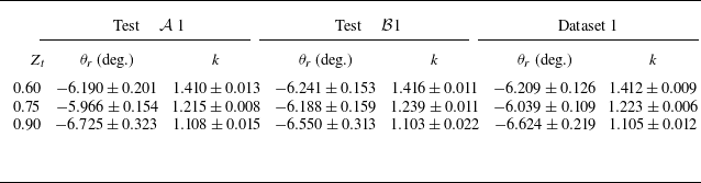
Extrapolated values of parameters
 $\theta _{\textit{r}}$
and
 $k$
with corresponding expanded uncertainties with 95 % confidence level.

The extrapolation procedure is first applied to tests
 $\mathcal{A}$
1 and
 $\mathcal{B}$
1 separately, with Mach numbers computed from the measured static pressures. The obtained approximating curves are shown in figure 13 for the same values of the compressibility factor considered in the previous sections. The extrapolated values of parameters
 $\theta _{\textit{r}}$
and
 $k$
and their expanded uncertainties with 95 % confidence level are reported in table 2, together with results obtained by considering the entire dataset 1, namely combining tests
 $\mathcal{A}$
1 and
 $\mathcal{B}$
1. Values of
 $\theta _{\textit{r}}$
and
 $k$
are in very good agreement both between the two tests and in the combined case. As expected, values of
 $\theta _{\textit{r}}$
show a small dependence on non-ideality, while a clear pattern is observed for parameter
 $k$
. Since
 $k=1$
corresponds to the ideal-gas solution, decreasing values of
 $k$
are found for increasing
 $Z_{\textit{t}}$
.
Extrapolation of the reference flow deflection
 $\theta _{\textit{r}}$
from experimental data of tests (a)
 ${\mathcal{A}}1$
and (b)
 $\mathcal{B}$
1, for different values of the compressibility factor
 $Z_{\textit{t}}$
. Experimental Mach numbers are computed from the measured static pressures. Corresponding total thermodynamic quantities are reported in table 1.

Given the good agreement of extrapolated parameters between the different tests, the complete dataset 1 is examined for the computation of the Prandtl–Meyer function, whose values are reported in figure 14(a). Mach number measurements from both pressure taps and schlieren images are considered, providing measurements of the Prandtl–Meyer function up to approximately 35
 $^\circ$
. Experimental results are compared to the theoretical solution obtained by integrating (1.5) under Span–Wagner thermodynamics. Measurements from both pressure taps and schlieren visualisations are in good agreement with theoretical results, showing a clear dependence of the Prandtl–Meyer function on non-ideality. The parity plot in figure 14(b) also shows a maximum deviation of 10 % from theoretical results.
Prandtl–Meyer function measurements obtained from experimental data for dataset 1, for different values of the compressibility factor
 $Z_{\textit{t}}$
. (a) Experimental measurements are compared to the theoretical solution of the Prandtl–Meyer function. (b) A parity plot shows the percentage deviation between experimental and theoretical values. Total thermodynamic quantities corresponding to the values of
 $Z_{\textit{t}}$
are reported in table 1.

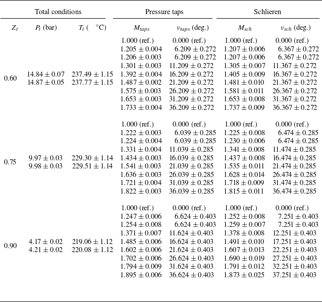
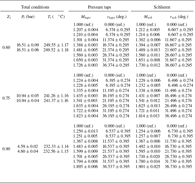
Numerical values of the measured Prandtl–Meyer function at different thermodynamic conditions are reported in table 3 for dataset 1, and table 4 for dataset 2. The usual three values of the compressibility factors at total conditions
 $Z_{\textit{t}} = 0.60, 0.75, 0.90$
are considered. For each of them, total pressure
 $P_{\textit{t}}$
and total temperature
 $T_{\textit{t}}$
are reported with the corresponding expanded uncertainties (see also table 1). In the columns of tables 3 and 4 reporting total conditions
 $P_t$
and
 $T_t$
, the first row refers to test
 $\mathcal{A}$
, and the second row to test
 $\mathcal{B}$
, for each value of
 $Z_t$
. Measured Mach numbers and reconstructed values of the Prandtl–Meyer function are then reported from both pressure taps and schlieren measurements. The reference condition (ref.) used for the definition of the Prandtl–Meyer function (i.e.
 $\nu = 0$
for
 $M=1$
) is reported in the first row for clarity, for each values of
 $Z_{\textit{t}}$
. Note also that the following two rows refer both to measurements in the uniform region 0 from different tests, therefore nearly the same values are found, as expected. Moreover, for completeness, an additional table is provided in Appendix B (see table 5), summarising all the measurements obtained during the experimental campaign. Table 5 reports values of the Mach number, the static-to-total pressure ratio and the Prandtl–Meyer function from both datasets, based on measurements acquired through pressure taps and schlieren images. Additional data, derived from the analytical expression of the Prandtl–Meyer function presented in § 4.4, are also included.
Experimental measurements from dataset 1. Both pressure taps and schlieren measurements are considered. The reference condition (ref.) for the definition of the Prandtl–Meyer function is also reported for clarity.

Experimental measurements from dataset 2. Both pressure taps and schlieren measurements are considered. The reference condition (ref.) for the definition of the Prandtl–Meyer function is also reported for clarity.

5. Concluding remarks
Prandtl–Meyer expansions were observed experimentally in the non-ideal compressible flow regime for siloxane fluid MM. Planar expansions at sharp convex corners were generated for discrete flow deflections
 $\theta$
from 5
 $^\circ$
to 30
 $^\circ$
, for varying stagnation thermodynamic conditions. Independent static pressure and Mach number measurements were used to characterise the flow evolution throughout the expansions, revealing increasing non-ideal thermodynamic effects while departing from dilute-gas conditions. For all the observed operating conditions, experimental results agreed well with Prandtl–Meyer theory, complemented with a thermodynamic model accounting for non-ideal behaviour. The role of the compressibility factor at total conditions
 $Z_{\textit{t}}$
as a similarity parameter for isentropic expansions of molecularly complex fluids was confirmed by comparing results at different thermodynamic conditions featuring the same values of
 $Z_{\textit{t}}$
. An approximate analytical expression of the Prandtl–Meyer function dependency on the Mach number was formulated and used to extrapolate from the experimental data a reference condition necessary for a correct definition of the Prandtl–Meyer function
 $\nu$
. Experimental values of
 $\nu$
up to approximately 35
 $^\circ$
were then extracted from the measured data. The obtained results compared well with theoretical predictions, providing the first experimental measurements of the Prandtl–Meyer function in the non-ideal compressible regime. The Prandtl–Meyer function reported in the present work is not limited to centred expansion fans shown here, and it can be used in all two-dimensional supersonic isentropic steady flows.
Acknowledgements
The authors wish to thank M. Zocca, C.C. Conti and A. Spinelli for their help in the design and data processing of the experiments, and for their contribution to the experimental campaign here reported.
Declaration of interests
The authors report no conflict of interest.
Appendix A. The TROVA experimental facility
A more detailed description of the TROVA facility and its components is provided here to support the understanding of the experimental campaign. A schematic of the plant is shown in figure 15, and a picture of the settling chamber and the test section is shown in figure 16. Before each test, the HPV is charged with a controlled amount of liquid MM, which is heated and vapourised by means of electric heaters. The LPV and all components of the test rig are brought to the saturation pressure of MM at room temperature (
 $\sim50$
mbar). All pipelines and valves connecting the two reservoirs, including the settling chamber and the test section, are heated to the same temperature as the HPV, to prevent fluid condensation during the flow discharge. The test is started by opening two valves, identified as V3 and ‘Main control valve’ in the schematic. The working fluid flows from the HPV to the LPV through the settling chamber, where total thermodynamic quantities are measured, and the test section, where static pressure measurements and schlieren visualisations are acquired. After the test, the vapour is condensed in the LPV and subsequently pumped back to the HPV to prepare the next experiment.
Tabulated values of the Prandtl–Meyer function for three different values of the compressibility factor
 $Z_{\textit{t}}$
, for both the examined datasets. Values of the Mach number, the static-to-total pressure ratio and the Prandtl–Meyer function are presented and distinguished among data of type Schlieren, Taps and Model, where the model is defined in § 4.4.

Layout of the TROVA plant. The HPV and LPV are highlighted, together with the settling chamber (in blue) and the test section (in green). The flow direction is also specified.

Spatial arrangement of the settling chamber and the test section of the TROVA. The flow direction is specified.

Appendix B. Tabulated values of the Prandtl–Meyer function
This appendix reports in table 5 the values of the main measurements obtained during the experimental campaign described in this work. Data are classified based on the compressibility factor evaluated at total conditions
 $Z_{\textit{t}}$
, which is reported with its expanded uncertainty, computed by the measured total pressure and temperature (see table 1). Mach number
 $M$
, static-to-total pressure ratio
 $P/P_{\textit{t}}$
, and the Prandtl–Meyer function
 $\nu$
are then reported. Three types of data are considered, referred to as types Schlieren, Taps and Model in the table. The first are experimental measurements obtained from schlieren images. The Mach number is directly measured from the slope of the characteristic lines in the schlieren frames. The static pressure is computed as
 $P = P(h,s)$
under Span–Wagner thermodynamics, where the entropy
 $s$
is retrieved from the measured stagnation quantities as
 $s = s(P_{\textit{t}}, T_{\textit{t}})$
, and the static enthalpy
 $h$
is found by solving the implicit nonlinear equation (4.2). On the other hand, for data identified as type Taps, static pressure is directly measured by pressure taps, and the corresponding Mach number is computed as in (4.1). In both cases, the Prandtl–Meyer function is retrieved by following the procedure described in § 4.4. For schlieren and pressure taps measurements, the corresponding dataset (1 or 2) is specified in the table. Expanded uncertainties with 95 % confidence level are obtained by following a Monte Carlo approach. Additional data are listed in the table and identified as data of type Model. They uniformly span Mach numbers between 1 and 2. For these data, the corresponding static pressure is found as for the schlieren measurements, while the Prandtl–Meyer function is computed based on the model described in § 4.4, i.e.
 $\nu = k\,\nu _{\textit{PIG}}(M)$
, with the value of
 $k$
defined in table 2 for dataset 1. Although these selected Mach numbers are not affected by uncertainties, the experimental uncertainties of the total quantities and the parameter
 $k$
are propagated, providing uncertainties of the pressure ratio and the Prandtl–Meyer function. Note that for
 $M=1$
, the Prandtl–Meyer function is arbitrarily set to
 $\nu = 0$
as discussed in § 4.4.