1 Introduction
In the last two decades, synthetic jets have attracted a considerable amount of research (e.g. Smith & Glezer Reference Smith and Glezer1998; Glezer & Amitay Reference Glezer and Amitay2002; Cattafesta & Sheplak Reference Cattafesta and Sheplak2011; O’Farrell & Dabiri Reference O’Farrell and Dabiri2014). Both experimental and numerical studies have focussed on the development of actuators, the formation and evolution of synthetic jets and on flow control applications. A typical synthetic jet actuator (SJA) consists of a cavity bounded by a diaphragm and an orifice. An oscillatory motion of the diaphragm drives a time-periodic flow through the orifice. Synthetic jets have the unique feature that they consist entirely of the working fluid of the flow system in which they are deployed. This creates a zero-net-mass-flux flow that has non-zero streamwise momentum. A large operational difference between continuous and synthetic jets is that the latter do not need an external fluid supply and therefore can be easily integrated in complex geometries, making them attractive actuators for flow control. Applications of synthetic jets, such as separation control (Dandois, Garnier & Sagaut Reference Dandois, Garnier and Sagaut2007), turbulent boundary layer control (Rathnasingham & Breuer Reference Rathnasingham and Breuer2003; Canton et al. Reference Canton, Örlü, Chin, Hutchins, Monty and Schlatter2016), virtual aeroshaping (Mittal & Rampunggoon Reference Mittal and Rampunggoon2002), thrust vectoring (Smith & Glezer Reference Smith and Glezer2002; Luo & Xia Reference Luo and Xia2005), heat transfer (Persoons, O’Donovan & Murray Reference Persoons, O’Donovan and Murray2009) or propulsion (Athanassiadis & Hart Reference Athanassiadis and Hart2016), include, but are not limited to, applications with a cross-flow. For most of these applications, the specific direction of the synthetic jet is important. For example, consider the control of large-scale structures in turbulent wall-bounded flows as introduced by Schoppa & Hussain (Reference Schoppa and Hussain1998) and re-analysed by Canton et al. (Reference Canton, Örlü, Chin, Hutchins, Monty and Schlatter2016). This control depends on direct interactions between these large-scale structures and controlled vortices. Steering of vortices using vectoring of a synthetic jet enables the precise targeting of these structures. Another example is propulsion using pulsed jets as investigated by Athanassiadis & Hart (Reference Athanassiadis and Hart2016). Vectoring these jets would vector the resultant thrust and add a steering mechanism to this method of propulsion.
As outlined below, in this study two parallel synthetic jets are placed side-by-side in quiescent air. Previous studies have looked at circular in-line twin synthetic jets issuing in a laminar boundary layer cross-flow, see for example Wen, Tang & Duan (Reference Wen, Tang and Duan2015). In practical applications, such as turbulent boundary layer control or separation control, it is often desirable to cover a large spanwise length, making rectangular jets more suitable than their circular equivalents. In order to perform detailed measurements of the fundamental vectoring mechanisms – not overshadowed by a cross-flow – measurements are performed in quiescent air. This is not only useful for applications in absence of a cross-flow (such as thrust vectoring), but will also give valuable insight into the effect of different parameters on the vectoring behaviour, which may be applied in subsequent cross-flow studies.
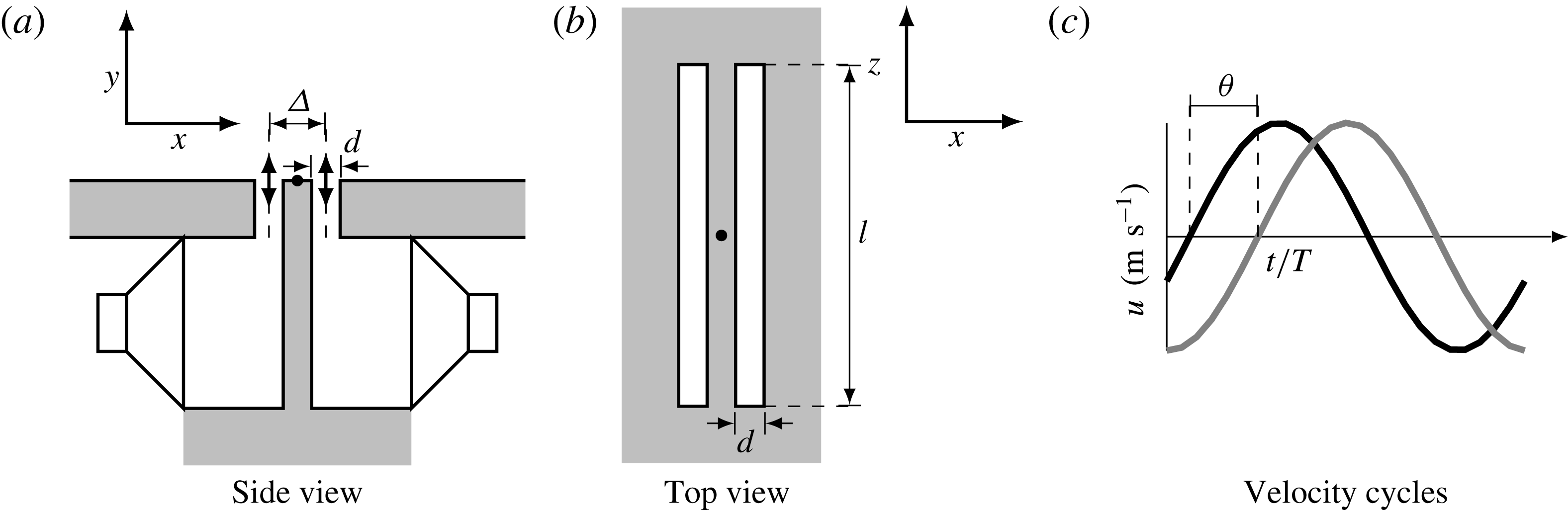
Disregarding the internal flow and dimensions of the actuator, the geometry for rectangular orifice jets is described by the slot length,
 $l$
(m), and width,
 $d$
(m). A single synthetic jet is actuated by a sinusoidal signal with frequency
 $f$
(Hz) and amplitude
 $A$
(
 $\text{V}_{pp}$
). It is assumed that this leads to a sinusoidal jet centreline velocity,
 $u$
(
 $\text{m}~\text{s}^{-1}$
), given by
 $$\begin{eqnarray}u(t)=u_{max}\sin (2\unicode[STIX]{x03C0}tf+\unicode[STIX]{x1D703}),\end{eqnarray}$$
with
 $u_{max}$
(
 $\text{m}~\text{s}^{-1}$
) the maximum velocity and
 $\unicode[STIX]{x1D703}$
(degrees) the phase of the jet. The start of a velocity cycle is defined as the onset of blowing. Following Smith & Glezer (Reference Smith and Glezer1998), the mean blowing velocity,
 $\bar{u}$
(
 $\text{m}~\text{s}^{-1}$
), is used as a representative velocity, defined as
 $$\begin{eqnarray}\bar{u}=\frac{1}{T}\int _{0}^{T/2}u(t)\,\text{d}t=\frac{1}{T}\int _{0}^{T/2}u_{max}\sin (2\unicode[STIX]{x03C0}t/T)\,\text{d}t=\frac{u_{max}}{\unicode[STIX]{x03C0}},\end{eqnarray}$$
with
 $T=1/f$
(s) the period of the signal. It should be noted that other representative velocities are used throughout the literature, most notably the momentum flow velocity,
 $U_{0}$
(
 $\text{m}~\text{s}^{-1}$
), as defined by Cater & Soria (Reference Cater and Soria2002), which relates to the mean blowing velocity as
 $U_{0}=\bar{u}\unicode[STIX]{x03C0}/\sqrt{2}$
.
The flow of a single synthetic jet can be characterized using three dimensionless parameters (Glezer & Amitay Reference Glezer and Amitay2002): the aspect ratio, the Strouhal number and the Reynolds number, defined as
 $$\begin{eqnarray}\displaystyle & \displaystyle AR=\frac{l}{d}, & \displaystyle\end{eqnarray}$$
 $$\begin{eqnarray}\displaystyle & \displaystyle St=\frac{fd}{\bar{u}}, & \displaystyle\end{eqnarray}$$
 $$\begin{eqnarray}\displaystyle & \displaystyle Re=\frac{\bar{u}d}{\unicode[STIX]{x1D708}}, & \displaystyle\end{eqnarray}$$
 $\unicode[STIX]{x1D708}$
(
 $\text{m}^{2}~\text{s}^{-1}$
) the kinematic viscosity.
In the limit of infinite aspect ratio, the flow can be assumed two-dimensional. For finite aspect ratio jets, edge effects and three-dimensional jet development play a role. However, results obtained by Van Buren, Whalen & Amitay (Reference Van Buren, Whalen and Amitay2014) for aspect ratios of
 $AR=6{-}18$
, indicate that edge effects do not reach the central plane up to a distance of approximately
 $y/d<AR/2$
. In the present research a near field up to this distance is defined within which three-dimensional effects on the flow in the central plane are assumed negligible.
Holman et al. (Reference Holman, Utturkar, Mittal, Smith and Cattafesta2005) proposed and validated a formation criterion for synthetic jets. They demonstrated that for
 $St>1/\unicode[STIX]{x03C0}$
vortices do not travel far enough from the actuator and are ingested back into the orifice during the suction phase. Therefore, to create a synthetic jet, it is important to keep the Strouhal number below
 $St=1/\unicode[STIX]{x03C0}$
.
When two actuators are placed next to each other at a spacing
 $\unicode[STIX]{x1D6E5}$
(m), as presented schematically in figure 1, vectoring of the jets can be achieved by applying a phase difference
 $\unicode[STIX]{x1D703}$
(degrees) between the driving signals (Smith & Glezer Reference Smith and Glezer2005). This expands the number of dimensionless parameters to five, since the phase difference (
 $\unicode[STIX]{x1D703}$
) and dimensionless spacing between the actuators (
 $\unicode[STIX]{x1D6E5}/d$
) also become important alongside the above-mentioned three parameters.
Schematic of synthetic jet actuator set-up, orientation and velocity cycle. The dots in (a) and (b) indicate the origin of the coordinate system.

A very limited body of literature exists on the influence of these five parameters on the vectoring of parallel synthetic jets. Smith & Glezer (Reference Smith and Glezer2005) investigated experimentally the vectoring of parallel synthetic jets by varying the phase difference for a single aspect ratio (
 $AR=150$
), Strouhal number (
 $St=0.03$
), Reynolds number (
 $Re=311$
) and spacing (
 $\unicode[STIX]{x1D6E5}/d=3.3$
). The authors demonstrated that, in the absence of a phase difference, a merged synthetic jet is formed with the same centreline velocity as a single jet, but more than twice the entrained fluid of a single jet. When a phase difference is introduced between the driving signals, the combined jet is vectored towards the actuator leading in phase. The vectoring angle increases with the phase difference, until the jet is fully attached to the surface. Vortex trajectories were tracked using phase-averaged vorticity concentrations. The authors demonstrated that the vortex trajectories are influenced by the velocity field in the vicinity of the actuators.
Luo & Xia (Reference Luo and Xia2008) carried out similar experiments, varying the phase difference for a single aspect ratio, Strouhal number, Reynolds number and spacing (
 $\unicode[STIX]{x1D6E5}/d=3.5$
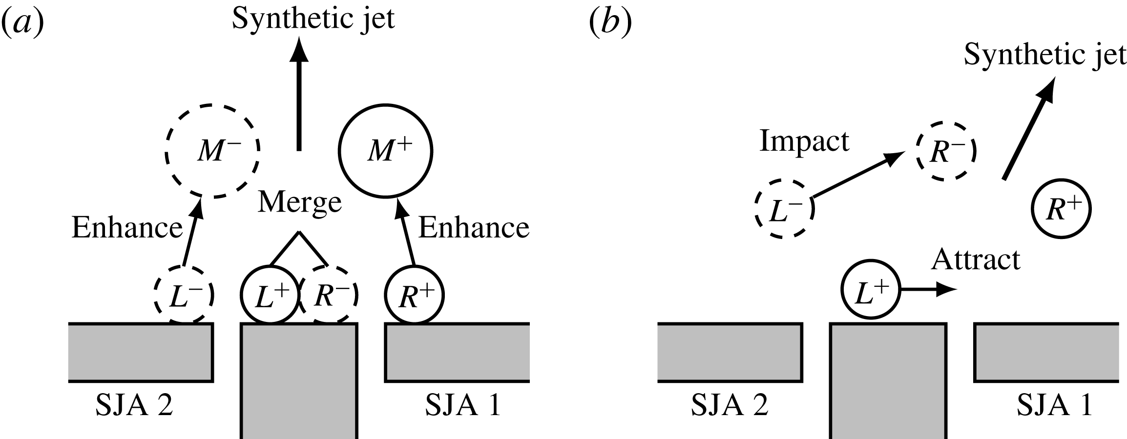
, slot length and jet velocity not mentioned). They showed that the merged jet vectors towards the actuator leading in phase, in agreement with the findings of Smith & Glezer (Reference Smith and Glezer2005). The authors proposed an interaction mechanism, presented in figure 2, explaining the enhancing and vectoring mechanisms of the interacting synthetic jets, based on vortex trajectories. In absence of a phase difference (see figure 2
a), two closely symmetric vortex pairs
 $L^{+}L^{-}$
and
 $R^{+}R^{-}$
are formed at the orifice exits. The lower pressure accompanying the vortex pairs makes them attract each other which leads to a merged vortex pair,
 $M^{+}M^{-}$
. When the actuator on the right is leading in phase (see figure 2
b),
 $R^{+}R^{-}$
is leading
 $L^{+}L^{-}$
. The trailing vortex pair is attracted by the low pressure in the wake of the leading vortex pair. The leading vortex pair slows down due to friction and entrainment of surrounding fluid, causing the trailing vortex pair to impinge upon the leading vortex pair. This transfers momentum in the direction towards the leading vortex pair, resulting in a merged jet in the direction of the actuator leading in phase.
Interaction between synthetic jets, redrawn from Luo & Xia (Reference Luo and Xia2008). Synthetic jets in absence of a phase difference, leading to an enhanced merged jet (a) and synthetic jets with a phase difference, leading to a vectored jet (b).

The present research will expand the analyses by Smith & Glezer (Reference Smith and Glezer2005) and Luo & Xia (Reference Luo and Xia2008) by investigating experimentally the influence of the Strouhal number, Reynolds number, phase difference and spacing on the vectoring of parallel synthetic jets. This increases the number of investigated parameters from one (phase difference) to four, only leaving the aspect ratio out of consideration. The fixed aspect ratio will be chosen large enough to enable the assumption that three-dimensional effects on the vectoring behaviour are negligible.
Results from both qualitative and quantitative analyses are presented. The qualitative analysis will first show the variation of time-averaged flow fields with Strouhal number for a fixed Reynolds number, phase difference and spacing. This is followed by a discussion on the influence of Strouhal number, identifying the exact mechanisms – using vortex tracking – that cause two distinct regimes of vectoring behaviour in Strouhal number space. Next, time-averaged flow fields for varying Reynolds number with a fixed phase difference and spacing are presented to show the (lack of) influence of the Reynolds number on the vectoring of parallel synthetic jets. The parametric variation is completed by varying the phase difference and spacing for a fixed Strouhal number and Reynolds number. For the quantitative analysis, parameters related to the direction and strength of the jet are defined. A quantitative analysis is performed on the same variations as the qualitative analysis (i.e. covering parametric variations of the Strouhal number, Reynolds number, phase difference and spacing). Using these results a new vectoring mechanism is proposed, explaining the vectoring behaviour for the full parameter space.
2 Experimental set-up and procedures
2.1 Description of the synthetic jet actuator
A Visaton SC 8 N speaker is used to actuate the synthetic jet actuator. This speaker has an impedance of 8
 $\unicode[STIX]{x03A9}$
with a rated power of 30 W (corresponding to
 $A=15.5~\text{V}_{pp}$
) and a frequency response between 70–20 000 Hz. Therefore, the synthetic jet actuator is operated with an amplitude limit of
 $A=15~\text{V}_{pp}$
and a lower frequency limit of
 $f=100$
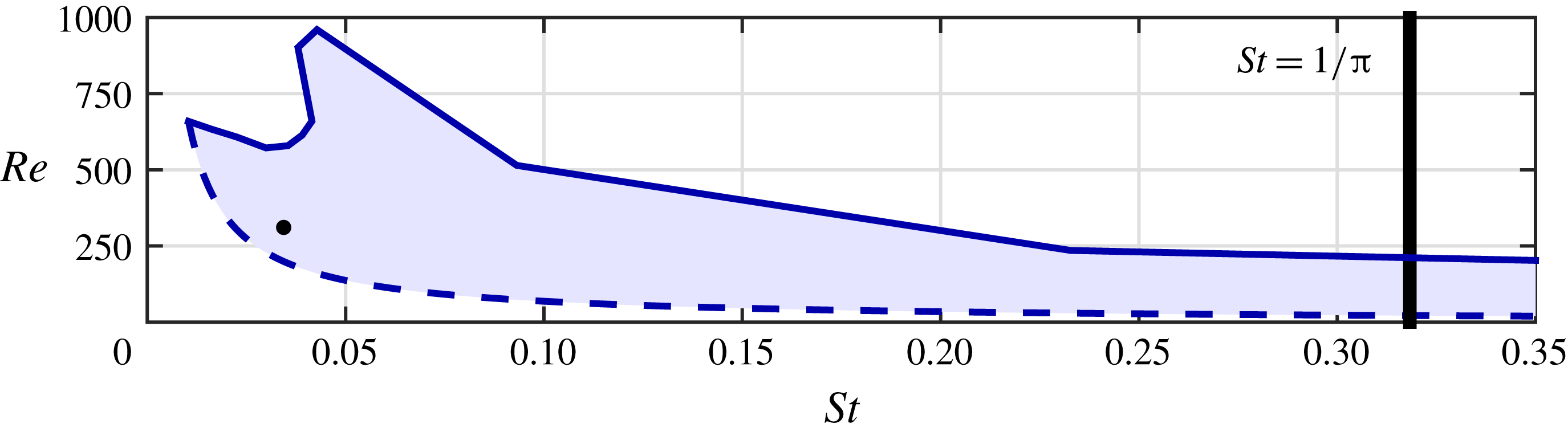
Hz. The average blowing velocity of the synthetic jet actuator is measured for multiple amplitudes and frequencies. All achievable values are represented by the shaded area in the graph of the Reynolds number versus the Strouhal number in figure 3. The upper amplitude limit of
 $A=15~\text{V}_{pp}$
shows a clear peak, corresponding to the Helmholtz resonance frequency of the actuator of approximately
 $f=600$
Hz.
The Strouhal number corresponding to the formation criterion is indicated by the thick solid line. The operating conditions for Smith & Glezer (Reference Smith and Glezer2005) (
 $Re=311$
,
 $St=0.03$
) are indicated by the black dot.
Actuator response in terms of Strouhal and Reynolds numbers for the actuator used in the present research. The shaded area shows the achievable values for the actuator, limited by the maximum amplitude of
 $A=15~\text{V}_{pp}$
and the minimum frequency of
 $f=100$
Hz, indicated by the solid and dashed lines respectively. The formation criterion is indicated by the thick solid line. The black dot indicates the operating conditions in Smith & Glezer (Reference Smith and Glezer2005).

Two identical synthetic jet actuators are placed side-by-side, parallel along the length of their orifices, as presented in figure 1. The slot width is
 $d=1$
mm and the slot length is
 $l=13$
mm, resulting in an aspect ratio of
 $AR=13$
. The spacing can be varied between
 $\unicode[STIX]{x1D6E5}=2.0{-}3.0$
mm, measured from the centres, resulting in dimensionless spacings of
 $\unicode[STIX]{x1D6E5}/d=2.0{-}3.0$
. The actuators are milled from aluminium plates with nozzles produced by a ‘3D printer’. The accuracy of the 3D printing technique is 0.1 mm, leading to an estimated uncertainty in the spacing of
 $\unicode[STIX]{x1D716}_{\unicode[STIX]{x1D6E5}/d}=0.1$
. The actuators are flush mounted in a horizontal plate, with the slot exits perpendicular to the plate. The actuators have a volume of
 $1.85\times 10^{-5}~\text{m}^{3}$
and a neck length of 19.5 mm.
2.2 Measurement procedures
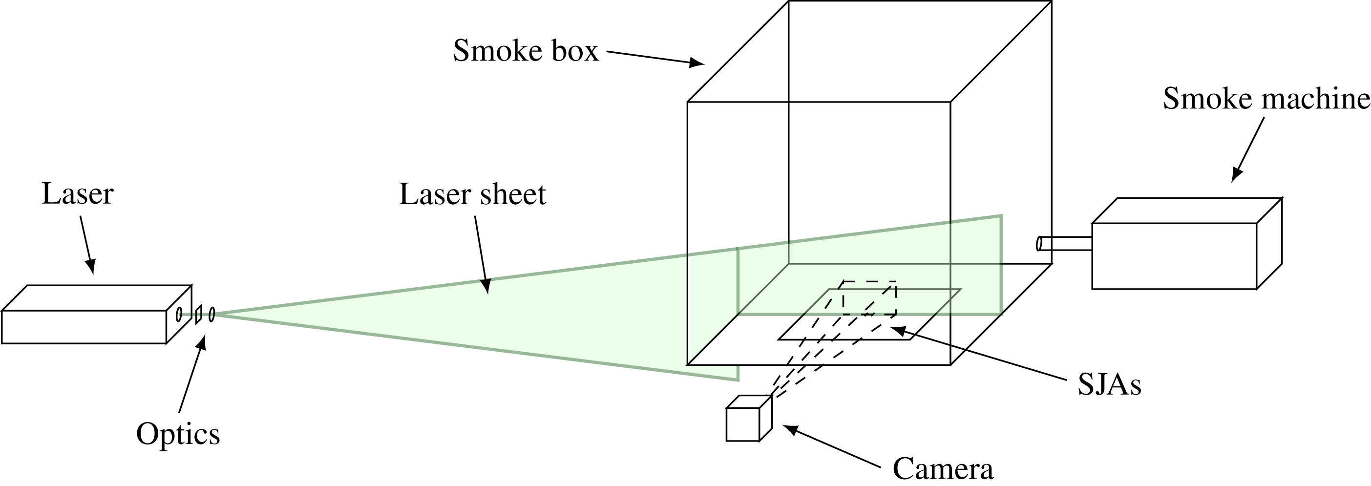
Measurements are performed using two-dimensional, two-component particle image velocimetry (PIV). Figure 4 presents a schematic of the experimental set-up. The PIV system consists of a Litron 200 mJ dual-pulse Nd-YAG laser and a LaVision Imager Pro LX 16MP camera that are phase locked to the driving signal using a National Instruments NI-DAQ. The laser sheet is positioned along the small symmetry axis of the slots, at
 $z/d=0$
as defined in figure 1(b). Seeding is provided by a Martín Magnum 1200 smoke machine, ejecting smoke particles with a mean diameter of
 $1~\unicode[STIX]{x03BC}\text{m}$
into a purpose-built Perspex box of length
 $400d$
on each side. Images are captured and processed using LaVision DaVis 8.2.2. Vectors are determined using a first step with a window size of
 $64\times 64$
pixels, followed by two steps of
 $32\times 32$
pixels with 50 % overlap, resulting in a resolution of one vector per 0.16 mm. The uncertainty in PIV is of the order of 0.05 pixels (Sciacchitano et al.
Reference Sciacchitano, Neal, Smith, Warner, Vlachos, Wieneke and Scarano2015), which corresponds to an uncertainty in the instantaneous velocity fields of
 $\unicode[STIX]{x1D716}_{u_{i}}=0.1~\text{m}~\text{s}^{-1}$
for the current work. For the phase-averaged, as well as for the time-averaged data, 100 image pairs are acquired, resulting in averages over 100 vector fields. This ensemble of 100 vector fields leads to an uncertainty in the repeatability of the same order as the uncertainty in the instantaneous velocity fields, showing adequate convergence for the analyses performed in the present research.
Phase-averaged flow fields are post-processed into swirling strength concentrations using MATLAB. Swirling strength is used to identify vortices and is defined as the imaginary part of the complex conjugate eigenvalues of the two-dimensional velocity gradient tensor as in Adrian, Christensen & Liu (Reference Adrian, Christensen and Liu2000). Vortices are identified as regions where the swirling strength exceeds a manually selected threshold. The advantage of using swirling strength over vorticity is that the former only identifies vortices, while the latter also depicts shear layers.
The synthetic jet velocity is determined using hot-wire anemometry. The estimated uncertainty in Strouhal number scales with
 $St/\bar{u}$
and ranges from
 $\unicode[STIX]{x1D716}_{St}=4\times 10^{-4}{-}18\times 10^{-4}$
. A repeatability study on the hot-wire data showed that the phase difference can be determined with an estimated uncertainty of
 $\unicode[STIX]{x1D716}_{\unicode[STIX]{x1D703}}=2$
degrees.
Schematic of experimental set-up. Synthetic jet actuators are located underneath the bottom plate of the smoke box.

3 Results and discussion
The results and discussion are divided into two sections that contain qualitative and a quantitative analyses, respectively. Both analyses start with a variation of Strouhal number for a fixed Reynolds number, phase difference and spacing. This is followed by a variation of Reynolds number for a fixed phase difference and spacing. The analyses are completed with the variation of phase difference and spacing for a fixed Strouhal number and Reynolds number. Both the qualitative and quantitative results are used to propose a new vectoring mechanism, amending and expanding the mechanism by Luo & Xia (Reference Luo and Xia2005), explaining vectoring of parallel synthetic jets for the full four-dimensional parameter space.
3.1 Qualitative analysis
Parametric variations are performed as described above. For the qualitative analysis, normalized time-averaged velocity maps of the local velocity magnitude (
 $|u|/\bar{u}$
) in the central plane (
 $z/d=0$
) are presented. Vector fields, indicating the local direction of the velocity are overlaid on these velocity magnitude maps. For clarity, only one in twenty vectors is displayed. The vectoring direction and direction of individual branches as defined in § 3.2 are indicated in the velocity maps by the solid and dashed blue lines respectively. Throughout the paper, phase differences are defined with the jet on the right leading in phase.
3.1.1 Dependency of vectoring behaviour on Strouhal number
The Strouhal number is varied for a fixed Reynolds number (
 $Re=342$
), phase difference (
 $\unicode[STIX]{x1D703}=150$
degrees, jet on the right leading in phase) and spacing (
 $\unicode[STIX]{x1D6E5}/d=2.0$
). The tested cases are indicated in the
 $St$
–
 $Re$
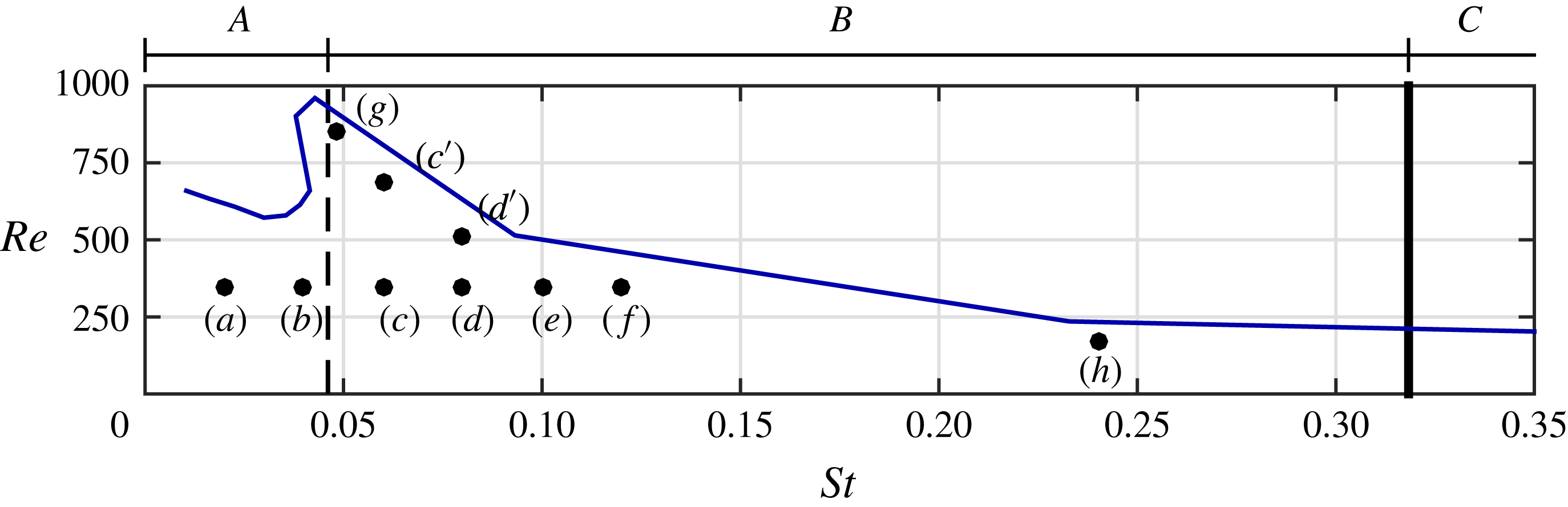
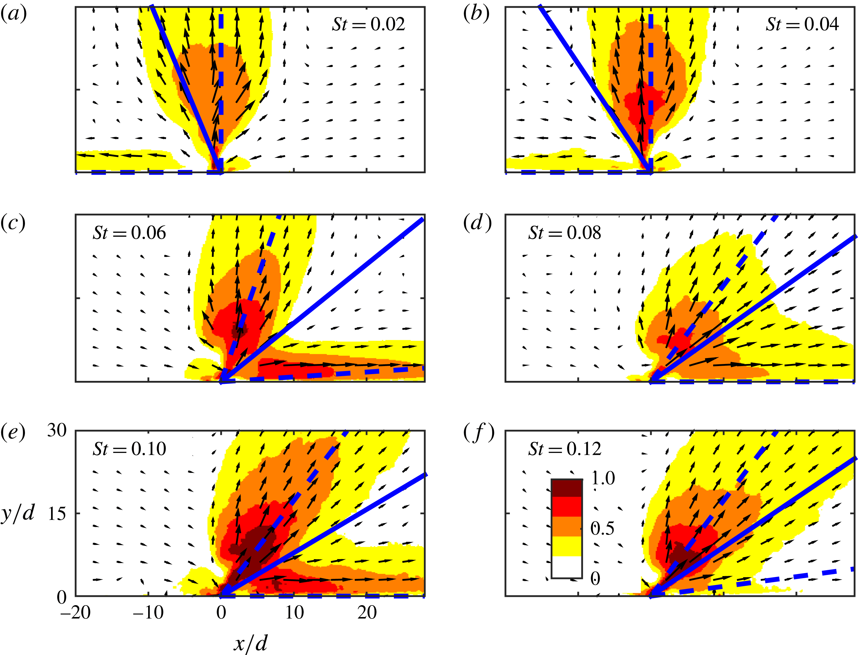
parameter space presented in figure 5. The annotations in this parameter space will be explained below. Normalized time-averaged velocity maps showing the vectoring behaviour for this variation are presented in figure 6(a–f), corresponding to cases (a–f) in figure 5.
Parameters for each case with the actuator response for
 $A=15$
 $\text{V}_{pp}$
shown as a reference. For each case
 $\unicode[STIX]{x1D6E5}/d=2.0$
and
 $\unicode[STIX]{x1D703}=150^{\circ }$
with the actuator on the right leading in phase.

Normalized time-averaged velocity maps,
 $|u|/\bar{u}$
, showing vectoring behaviour for different Strouhal numbers. For each case,
 $Re=342$
,
 $\unicode[STIX]{x1D6E5}/d=2.0$
and
 $\unicode[STIX]{x1D703}=150^{\circ }$
with the actuator on the right leading in phase. The solid and dashed blue lines indicate the vectoring direction and directions of the individual branches as defined in § 3.2. For clarity, only one in twenty vectors is displayed. Cases are indicated in the graph in figure 5.

In cases (a) and (b), presented in figures 6(a) and 6(b), a bifurcated synthetic jet is produced with one branch in the vertical direction and one branch in the direction towards the actuator that is lagging in phase. For higher Strouhal numbers, presented in figures 6(c–f), the jet is bifurcated into a strong branch in the vertical direction and a weaker branch in the direction towards the actuator leading in phase. For these cases (c–f), the included angle between the two branches of the jet visually decreases for increasing Strouhal number. This variation of included angle with Strouhal number is quantified in § 3.2.1.
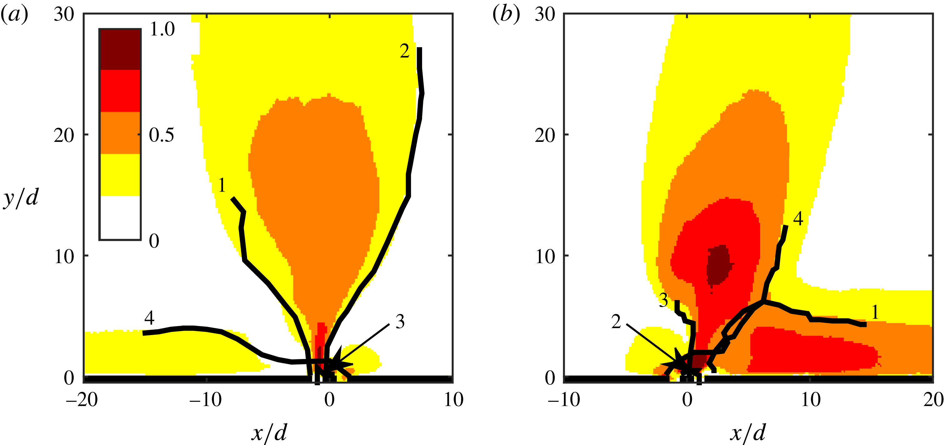
Following the vectoring mechanism based on vortices as proposed by Luo & Xia (Reference Luo and Xia2005), vortices for cases (a) and (c) are tracked to identify the mechanism causing the difference in vectoring direction of the horizontal branch. Vortices are tracked using phase-locked maps of the swirling strength. Instantaneous flow fields are captured phase locked to the driving signal at 12 equally spaced time intervals. Some vortices can be tracked over more than a single cycle, leading to vortex trajectories consisting of more than 12 points. Others break up within a single cycle, leading to trajectories consisting of less than 12 points. The resulting vortex trajectories are presented in figure 7. Vortex trajectories are numbered 1–4, according to the vortex starting positions from left to right in figure 7, i.e. the anticlockwise and clockwise vortices originating from the lagging actuator are labelled 1 and 2 respectively and the anticlockwise and clockwise vortices originating from the leading actuator 3 and 4.
Normalized time-averaged velocity maps,
 $|u|/\bar{u}$
, showing vortex trajectories for the
 $St=0.02$
(a) and
 $St=0.06$
(b) cases as shown in figure 6(a,c). Trajectories are numbered 1–4 for vortices originating from left to right, i.e. the anticlockwise (1) and clockwise (2) vortices originating from the lagging actuator and the anticlockwise (3) and clockwise (4) vortices from the leading actuator. Supplementary movies (http://dx.doi.org/10.1017/jfm.2016.559) showing these vortex trajectories using phase-locked vorticity maps are available with the online version of this paper as Movie 1 and Movie 2 for (a) and (b) respectively.

Figure 7 shows that the main difference between the
 $St=0.02$
and the
 $St=0.06$
cases is that different vortices are ingested into the neighbouring actuators. For the
 $St=0.02$
case, the anticlockwise vortex originating from the leading actuator, numbered 3, is ingested into the lagging actuator, while for the
 $St=0.06$
case the clockwise vortex originating from the lagging actuator, numbered 2, is ingested into the leading actuator. Upon ingestion of one of the vortices, the remaining vortex pair propagates in the vertical direction driven by its induced velocity, while the single vortex propagates along the surface driven by its own induced velocity reflected on the surface.
The relative position of the vortex trajectories on the velocity magnitude maps clearly indicates that the direction of both branches is governed by the vortex trajectories, as suggested in the literature by both Smith & Glezer (Reference Smith and Glezer2005) and Luo & Xia (Reference Luo and Xia2008). It should be noted that both figures 7(a) and 7(b) show that the direction of the vortex trajectories is determined within roughly
 $r/d=5$
, with
 $r$
(m) being the absolute distance of the vortex from the origin. This is within the near-field range of
 $r/d<AR/2$
as determined by Van Buren et al. (Reference Van Buren, Whalen and Amitay2014) where the behaviour of the jet can be considered to be two-dimensional (at least in the central plane).
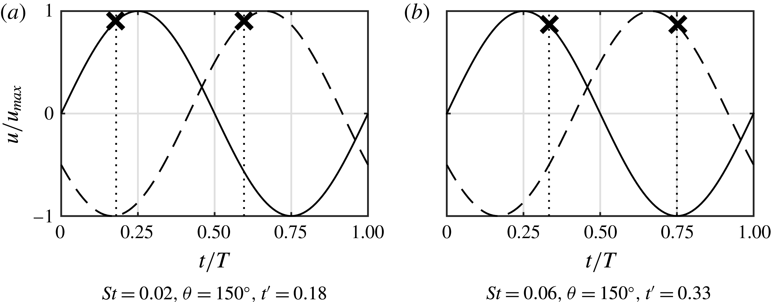
The only difference between these two cases is the Strouhal number and, therefore, they have the exact same (normalized) velocity cycles, as presented in figure 8. This implies that the only difference in velocity induced on newly created vortices by the suction of the neighbouring actuator is caused by the moment in the velocity cycle at which the vortex pairs are formed, which is defined as the pinch-off moment,
 $t^{\ast }/T$
.
Gharib, Rambod & Shariff (Reference Gharib, Rambod and Shariff1998) proposed a constant formation number at which pinch off occurs,
 $L/D\approx 4$
, where
 $L$
(m) is the stroke length and
 $D$
(m) is the diameter of the circular orifice. They assumed the physical process causing this constant formation number to be a maximum in total circulation attainable in the vortex ring. A numerical study by Rosenfeld, Rambod & Gharib (Reference Rosenfeld, Rambod and Gharib1998) demonstrates the invariance of this formation number to differences in the velocity programme and Reynolds number.
Velocity cycles with vortex pinch-off moments for equal phase differences but different Strouhal numbers. The continuous line represents the velocity as function of time for the leading actuator, the dashed line for the lagging actuator. Crosses indicate pinch-off time.

A study by O’Farrell & Dabiri (Reference O’Farrell and Dabiri2014) demonstrates that for non-axisymmetric orifices, the formation number still holds when expressed as
 $L/D_{eq}$
, where
 $D_{eq}$
(m) is the equivalent diameter of the orifice; the diameter of an axisymmetric orifice with the same cross-sectional area. For a rectangular orifice, the equivalent diameter is given by
 $$\begin{eqnarray}D_{eq}=2\sqrt{ld/\unicode[STIX]{x03C0}}=2d\sqrt{AR/\unicode[STIX]{x03C0}}.\end{eqnarray}$$
The instantaneous stroke length,
 $L(t)$
(m), is given by
 $$\begin{eqnarray}L(t)=\int _{0}^{t}u(t)\,\text{d}t=\int _{0}^{t}u_{max}\sin (2\unicode[STIX]{x03C0}t/T)\,\text{d}t=\frac{\bar{u}}{2f}(1-\cos (2\unicode[STIX]{x03C0}t/T)).\end{eqnarray}$$
Dividing the instantaneous stroke length by the equivalent diameter leads to
 $$\begin{eqnarray}L(t)/D_{eq}=\frac{\bar{u}}{fd}\frac{1-\cos (2\unicode[STIX]{x03C0}t/T)}{4\sqrt{AR/\unicode[STIX]{x03C0}}}=\frac{1}{St}\frac{1-\cos (2\unicode[STIX]{x03C0}t/T)}{4\sqrt{AR/\unicode[STIX]{x03C0}}}.\end{eqnarray}$$
For distinction between instantaneous values and limiting parameters, in the remainder of this paper the formation number (
 $L/D_{eq}$
) and pinch-off time (
 $t^{\ast }/T$
) are denoted as
 $L^{\prime }$
and
 $t^{\prime }$
respectively. According to (3.3), the pinch-off time,
 $t^{\prime }$
, at which the constant formation number,
 $L^{\prime }$
, is reached, is given by
 $$\begin{eqnarray}t^{\prime }=\cos ^{-1}\left(1-4L^{\prime }St\sqrt{AR/\unicode[STIX]{x03C0}}\right)/(2\unicode[STIX]{x03C0}).\end{eqnarray}$$
Equation (3.4) shows that, for a given geometry and constant formation number, the pinch-off time is a function of the Strouhal number only. This, for the first time, shows the direct link between pinch off and Strouhal number/aspect ratio.
In addition to the formation number, Aydemir, Worth & Dawson (Reference Aydemir, Worth and Dawson2012) proposed a limiting time scale at which pinch off occurs. Using sinusoidal forcing of a steady round jet, they found a limiting time of
 $t^{\prime }=1/3$
at which the vortex rings pinch off if the formation number is not reached before then. The authors attributed this limiting time to the change in sign of the jet acceleration, occurring at
 $t/T=0.25$
for a sinusoidal excitation.
It is assumed that the conditions in the present study are sufficiently similar to the literature and pinch off happens at either
 $L^{\prime }=4$
or
 $t^{\prime }=1/3$
, whichever occurs first. The boundary between these two regimes can be calculated from (3.4) as the Strouhal number for which the right-hand side equals
 $t^{\prime }=1/3$
. This Strouhal number is given by
 $$\begin{eqnarray}St=\frac{1-\cos (2\unicode[STIX]{x03C0}/3)}{4L^{\prime }\sqrt{AR/\unicode[STIX]{x03C0}}}=\frac{3}{32}\sqrt{\frac{\unicode[STIX]{x03C0}}{AR}}.\end{eqnarray}$$
Accordingly, the pinch-off time is given by
 $$\begin{eqnarray}\displaystyle \displaystyle t^{\prime }=\cos ^{-1}\left(1-16St\sqrt{AR/\unicode[STIX]{x03C0}}\right)/(2\unicode[STIX]{x03C0})\quad & \text{for}~\mathit{St}<\displaystyle \frac{3}{32}\sqrt{\displaystyle \frac{\unicode[STIX]{x03C0}}{AR}}, & \displaystyle\end{eqnarray}$$
 $$\begin{eqnarray}\displaystyle \displaystyle t^{\prime }=1/3\quad & \text{for}~\mathit{St}>\displaystyle \frac{3}{32}\sqrt{\displaystyle \frac{\unicode[STIX]{x03C0}}{AR}}. & \displaystyle\end{eqnarray}$$
It should be noted that pinch off is not qualitatively visible in the velocity field, nor in the vorticity field. As described by Gharib et al. (Reference Gharib, Rambod and Shariff1998), the pinch-off time is found by relating the circulation in a given vortex to the time at which this total circulation was produced by the jet.
Pinch-off times for both cases presented in figure 7 are calculated based on the above equations. For the
 $St=0.02$
and
 $St=0.06$
cases, pinch-off times are
 $t^{\prime }=0.19$
and
 $t^{\prime }=0.33$
respectively. The velocity cycles of both jets, with indicated pinch-off moments, are presented in figure 8. Figure 8(a) demonstrates that for
 $St=0.02$
, corresponding to the case in figure 7(a), the vortex pair originating from the actuator leading in phase pinches off while the actuator lagging in phase is near the peak of its suction cycle. This causes the leading vortex pair to be partly ingested into the lagging actuator and the resulting branch of the synthetic jet to be vectored in the direction towards the actuator lagging in phase as in figure 7(a). In contrast, figure 8(b) shows that for
 $St=0.06$
, corresponding to the case in figure 7(b), the vortex pair produced by the actuator lagging in phase pinches off while the actuator leading in phase is near the peak of its suction cycle. This causes the lagging vortex pair to be partially ingested into the leading actuator, forming a horizontal branch in the direction towards the actuator leading in phase, as in figure 7(b).
Equations (3.6) and (3.7) show that there is a limit for the Strouhal number, only depending on the aspect ratio, above which the pinch-off time is invariant. This limit, for the set-up in the present study, is indicated by the dashed line in figure 5. The range of Strouhal numbers below this limit, denoted as regime A, leads to a vectoring behaviour as presented in figure 6(a,b), for which a strong vertical branch and weak horizontal branch in the direction of the actuator lagging in phase are formed. The range of Strouhal numbers from this limit up to the formation criterion, denoted as regime B, leads to the vectoring behaviour presented in figure 6(c–f), for which a roughly vertical branch and a horizontal branch in the direction of the actuator leading in phase are formed. Above the formation criterion, in regime C, no synthetic jet is created. For the remainder of this paper, parameter variations within regime B only are considered.
It should be noted that the operating condition for Smith & Glezer (Reference Smith and Glezer2005) lies between cases (a) and (b) in figure 5. However, for their geometry the formation number, separating regimes A and B, occurs at
 $St=0.01$
. This implies that if their operating condition was to be met in the present research, it would lie in regime A, while for their research it was in regime B, meaning that the exact conditions cannot be reproduced in the present research.
3.1.2 Dependency of vectoring behaviour on Reynolds number
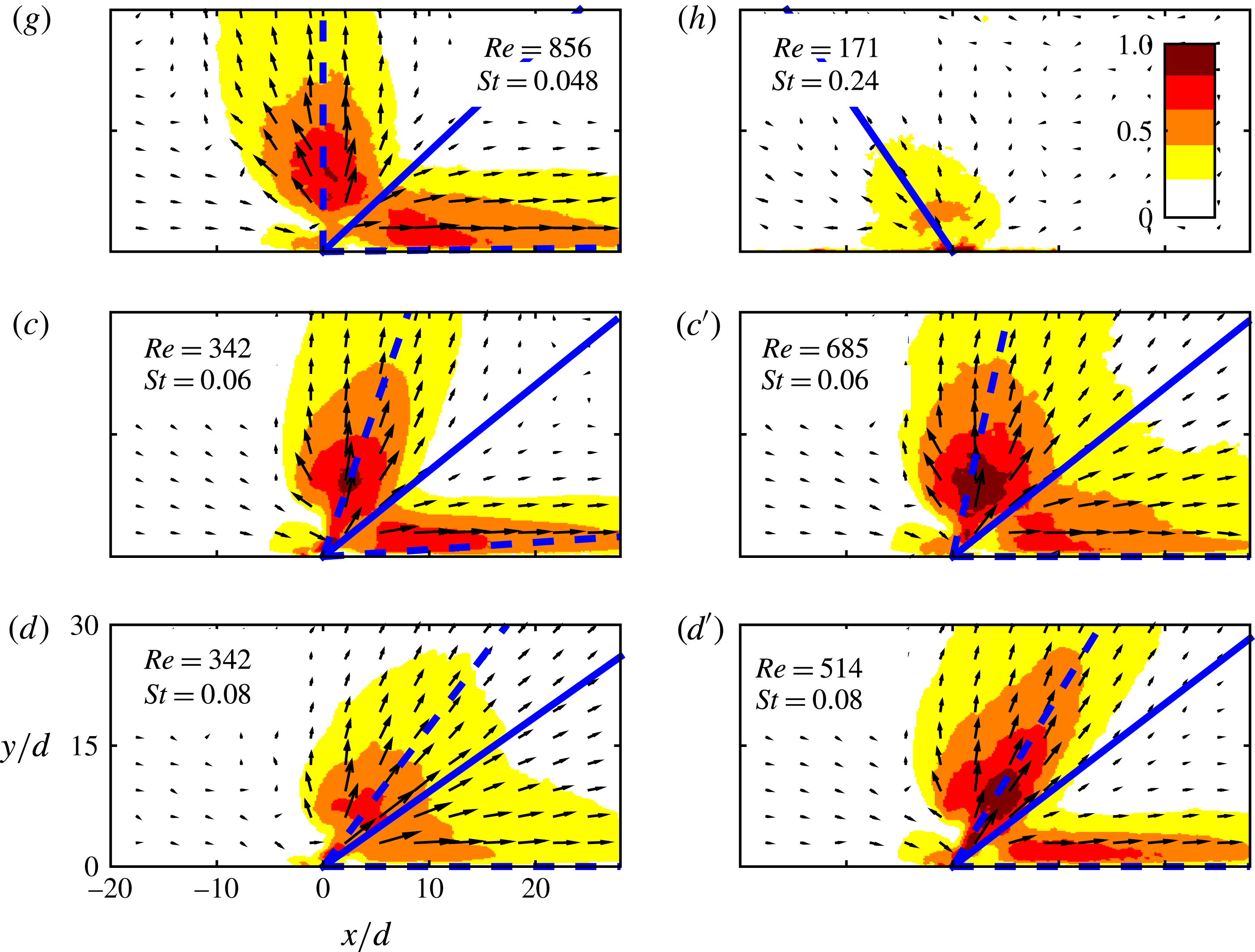
The Reynolds number is varied for a fixed phase difference (
 $\unicode[STIX]{x1D703}=150$
degrees, jet on the right is leading in phase) and spacing (
 $\unicode[STIX]{x1D6E5}/d=2.0$
). Note that these are the same phase difference and spacing as for the Strouhal variation discussed above. Cases are named (g), (h), (
 $c^{\prime }$
) and (
 $d^{\prime }$
) in order to build upon the six cases for the Strouhal variation and to stress that (
 $c^{\prime }$
) and (
 $d^{\prime }$
) have the same Strouhal numbers as (c) and (d) respectively. The location of the cases in the
 $St$
–
 $Re$
parameter space is indicated in figure 5. These cases are not taken at a fixed Strouhal number, but at a fixed frequency in an attempt to illustrate the relative importance of Strouhal number compared to Reynolds number.
Normalized time-averaged velocity maps,
 $|u|/\bar{u}$
, showing vectoring behaviour for different Reynolds and Strouhal numbers. For each case
 $\unicode[STIX]{x1D6E5}/d=2.0$
and
 $\unicode[STIX]{x1D703}=150^{\circ }$
with the actuator on the right leading in phase. The solid and dashed blue lines indicate the vectoring direction and directions of the individual branches as defined in § 3.2. For clarity, only one in twenty vectors is displayed. Cases are indicated in the graph in figure 5.

Normalized time-averaged velocity maps,
 $|u|/\bar{u}$
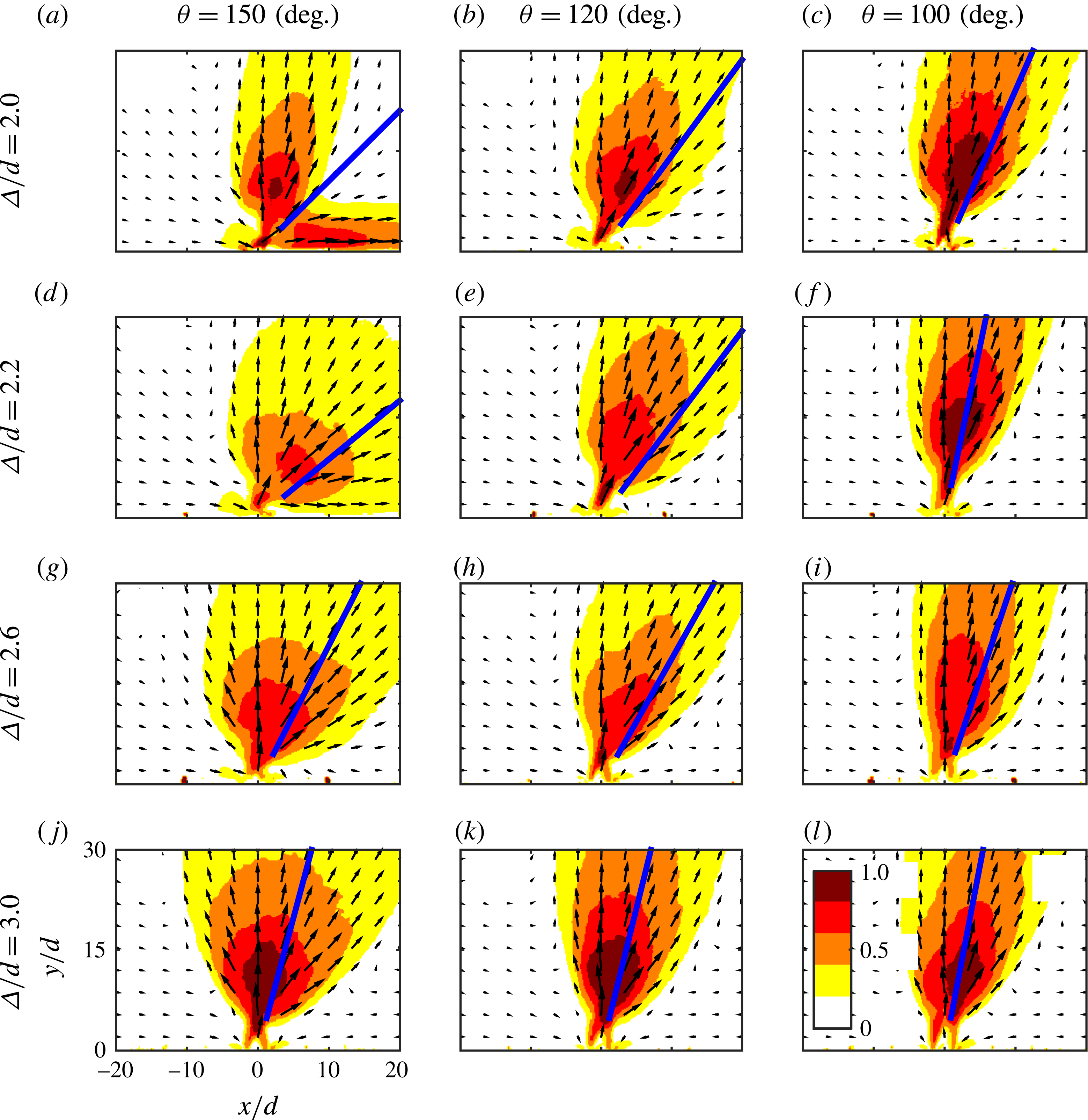
, showing vectoring behaviour for different phase differences and spacings. Vectoring directions as defined by (3.9) are indicated by the blue lines. For each case,
 $St=0.06$
,
 $Re=342$
and the actuator on the right is leading in phase. For clarity, only one in twenty vectors is displayed.

Normalized time-averaged velocity maps showing the vectoring behaviour for this variation are presented in figure 9. Variation of Reynolds number only, for a fixed Strouhal number, is present between cases (c) and (
 $c^{\prime }$
), as well as between cases (d) and (
 $d^{\prime }$
). Both combinations show very little influence of the Reynolds number on the vectoring behaviour, especially when considering the directions of the individual branches as well as the total vectoring direction. However, it can be seen that as the Reynolds number increases for a given Strouhal number, the momentum flux in each branch of the vectored jets also increases. This is made clearer in the quantitative analysis section.
Case (h) represents a scenario that is not only at a different Reynolds number, but also at a different Strouhal number than the other cases. This Strouhal number,
 $St=0.24$
, approaches the formation criterion, as is visible in the parameter space in figure 5. This causes a large part of the ejected fluid to be ingested back into the actuator during the suction part of the cycle. This is observed in figure 9(h) by the formation of a much weaker jet compared with the other cases.
3.1.3 Dependency of vectoring behaviour on phase difference and spacing
The phase difference and spacing are varied for a fixed Strouhal number (
 $St=0.06$
) and Reynolds number (
 $Re=342$
). These Strouhal and Reynolds numbers correspond to case (c) as presented in figures 6 and 9. This case is adequately far away from both the formation criterion and the formation number, suggesting that a strong synthetic jet is formed that vectors towards the actuator leading in phase. Vortex trajectories for the baseline case with
 $\unicode[STIX]{x1D6E5}/d=2.0$
and
 $\unicode[STIX]{x1D703}=150$
degrees are presented in figure 7(b). Five phase differences, ranging from
 $\unicode[STIX]{x1D703}=100$
degrees to
 $\unicode[STIX]{x1D703}=150$
degrees and six spacings, ranging from
 $\unicode[STIX]{x1D6E5}/d=2.0$
to
 $\unicode[STIX]{x1D6E5}/d=3.0$
are tested, yielding a parameter space of 30 points. A selection of the time-averaged velocity maps, showing the full range of observed vectoring behaviour, is presented in figure 10. Vectoring directions, defined by (3.9), are indicated by the thick blue lines.
Case (a), for
 $\unicode[STIX]{x1D6E5}/d=2.0$
and
 $\unicode[STIX]{x1D703}=150$
degrees, is the baseline case mentioned above. Interestingly, this is the only case that shows bifurcation. A mechanism describing bifurcation or merging of the two jets is presented in § 3.3.
The vectoring angle decreases for both a decreasing phase difference (left-to-right) and for an increasing spacing (top-to-bottom). Although these variations have a similar effect on the vectoring angle, they produce qualitatively different flow fields. Decreasing the phase difference, i.e. bringing the leading and lagging vortex pairs closer together, results in a more compact merged jet. On the other hand, increasing the spacing, i.e. increasing the horizontal distance between the leading and lagging vortex pairs, leads to a wider merged jet. The variation of vectoring angle with phase difference and spacing is quantified and further analysed below.
3.2 Quantitative analysis
To quantify the vectoring behaviour described above, the direction of individual branches,
 $\unicode[STIX]{x1D6FD}_{1}$
(degrees) and
 $\unicode[STIX]{x1D6FD}_{2}$
(degrees), the included angle between these branches,
 $\unicode[STIX]{x0394}\unicode[STIX]{x1D6FD}$
(degrees), the total vectoring angle of the flow,
 $\unicode[STIX]{x1D6FD}$
(degrees) and the normalized momentum flux,
 $J^{\prime }r/J_{0}$
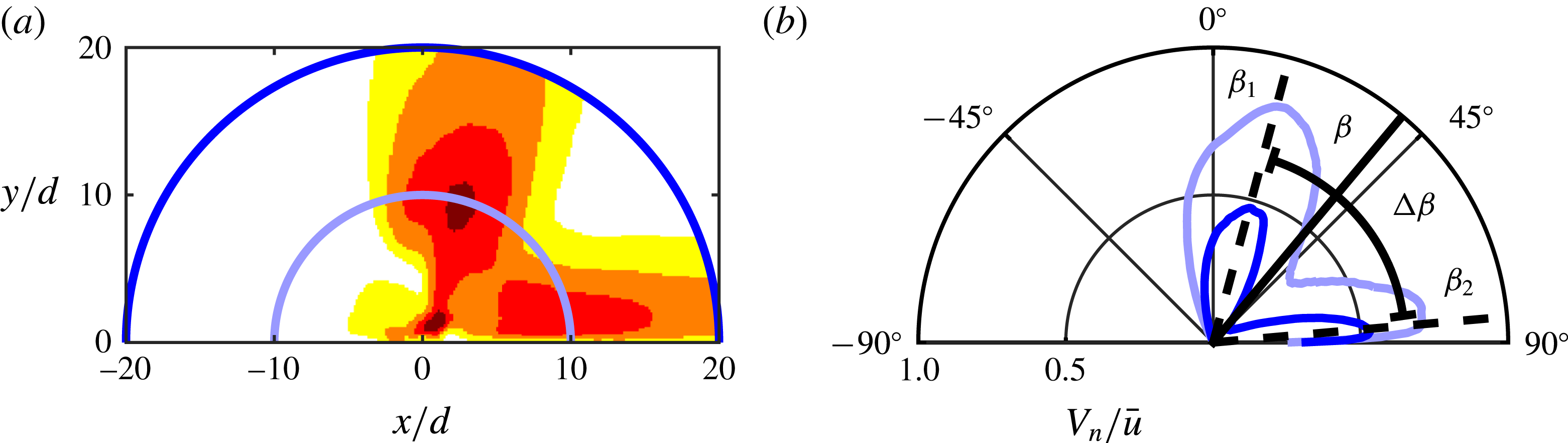
, are determined. The definition of these metrics is given using the example presented in figure 11. Figure 11(a) shows the velocity field corresponding to the case in figure 6(c) with two circles around the origin (
 $r/d=10$
and
 $r/d=20$
). The normalized normal velocity at these circles,
 $V_{n}/\bar{u}$
, as function of the angle with respect to the vertical axis is presented in figure 11(b). Note that in figure 11(a) only the velocity magnitude for
 $r/d<20$
is plotted, which is the part of the velocity used in the calculation of the vectoring angle.
Time-averaged velocity map for the case shown in figure 6(c) with circles at
 $r/d=10$
and
 $r/d=20$
(a) and the normalized normal velocities at these circles as function of the angle with respect to the vertical axis (b). The directions of both individual branches,
 $\unicode[STIX]{x1D6FD}_{1}$
and
 $\unicode[STIX]{x1D6FD}_{2}$
, are indicated in (b), along with the vectoring angle,
 $\unicode[STIX]{x1D6FD}$
and the included angle,
 $\unicode[STIX]{x0394}\unicode[STIX]{x1D6FD}$
.

The two bifurcated branches of the jet are clearly visible in the normal velocity as presented in figure 11(b). The direction of the individual branches is calculated from the angle at which the peaks are located. These peaks are detected with an estimated accuracy of one degree for 20 distances ranging from
 $r/d=10$
to
 $r/d=20$
. The means of these peaks give the vectoring angles of the individual branches,
 $\unicode[STIX]{x1D6FD}_{1}$
(degrees) and
 $\unicode[STIX]{x1D6FD}_{2}$
(degrees). A typical root mean square variation of less than one degree is associated with this mean. The uncertainty in the peak detection and root mean square variation of the peaks adds up to approximately
 $\unicode[STIX]{x1D716}_{\unicode[STIX]{x1D6FD}_{1,2}}=1.5$
degrees, which leads to an uncertainty of approximately
 $\unicode[STIX]{x1D716}_{\unicode[STIX]{x0394}\unicode[STIX]{x1D6FD}}=3$
degrees for the included angle,
 $\unicode[STIX]{x0394}\unicode[STIX]{x1D6FD}$
(degrees), which is defined as the angle between the two branches as indicated in figure 11(b), i.e.
 $$\begin{eqnarray}\unicode[STIX]{x0394}\unicode[STIX]{x1D6FD}=|\unicode[STIX]{x1D6FD}_{2}-\unicode[STIX]{x1D6FD}_{1}|.\end{eqnarray}$$
The vectoring angle is defined as the total direction of the flow, taking into account the flow within the circle
 $r/d=20$
only, which is the largest (half-)circle that fits in the velocity fields as can seen from figure 11(a). This circle is used to remove a bias towards the horizontal or vertical side that would be present if the field of view extended further in either direction. This defines the vectoring angle as
 $$\begin{eqnarray}\unicode[STIX]{x1D6FD}=\text{atan}\left(\sum V_{x}/\sum V_{y}\right),\end{eqnarray}$$
for summations over the area within the circle
 $r/d=20$
.
The uncertainty propagation of the velocity into the calculation of the vectoring angle leads to an uncertainty of less than 0.1 degree. The typical root mean square variation associated with determining the vectoring angle for different distances from the origin is approximately two degrees. Combining the uncertainty propagation of the velocity and the root mean square variation leads to an uncertainty estimation of approximately
 $\unicode[STIX]{x1D716}_{\unicode[STIX]{x1D6FD}}=2$
degrees.
The time-averaged momentum flux per unit depth,
 $J^{\prime }$
(
 $\text{kg}~\text{s}^{-2}$
), is calculated from the time-averaged velocity maps by integrating the normal velocity component over (half-) circles around the origin, i.e.
 $$\begin{eqnarray}J^{\prime }(r)=\int _{-90}^{90}\unicode[STIX]{x1D70C}V_{n}^{2}(r,\unicode[STIX]{x1D6FC})r\,\text{d}\unicode[STIX]{x1D6FC},\end{eqnarray}$$
with
 $\unicode[STIX]{x1D70C}$
(
 $\text{kg}~\text{m}^{-3}$
) the density of air,
 $V_{n}(r,\unicode[STIX]{x1D6FC})$
(
 $\text{m}~\text{s}^{-1}$
) the normal velocity with respect to the line of integration,
 $r$
(m) the distance from the origin and
 $\unicode[STIX]{x1D6FC}$
(degrees) the angle with respect to the vertical line
 $x=0$
. This momentum flux per unit depth is normalized by the momentum flux added to the flow,
 $J_{0}$
(
 $\text{kg}~\text{m}~\text{s}^{-2}$
), based on
 $A=ld$
and the momentum flow velocity,
 $U_{0}$
(
 $\text{m}~\text{s}^{-1}$
), as defined above. The normalized momentum flux per unit depth for the case with
 $St=0.06$
,
 $Re=342$
,
 $\unicode[STIX]{x1D6E5}/d=2.0$
and
 $\unicode[STIX]{x1D703}=150$
degrees is presented as function of
 $r/d$
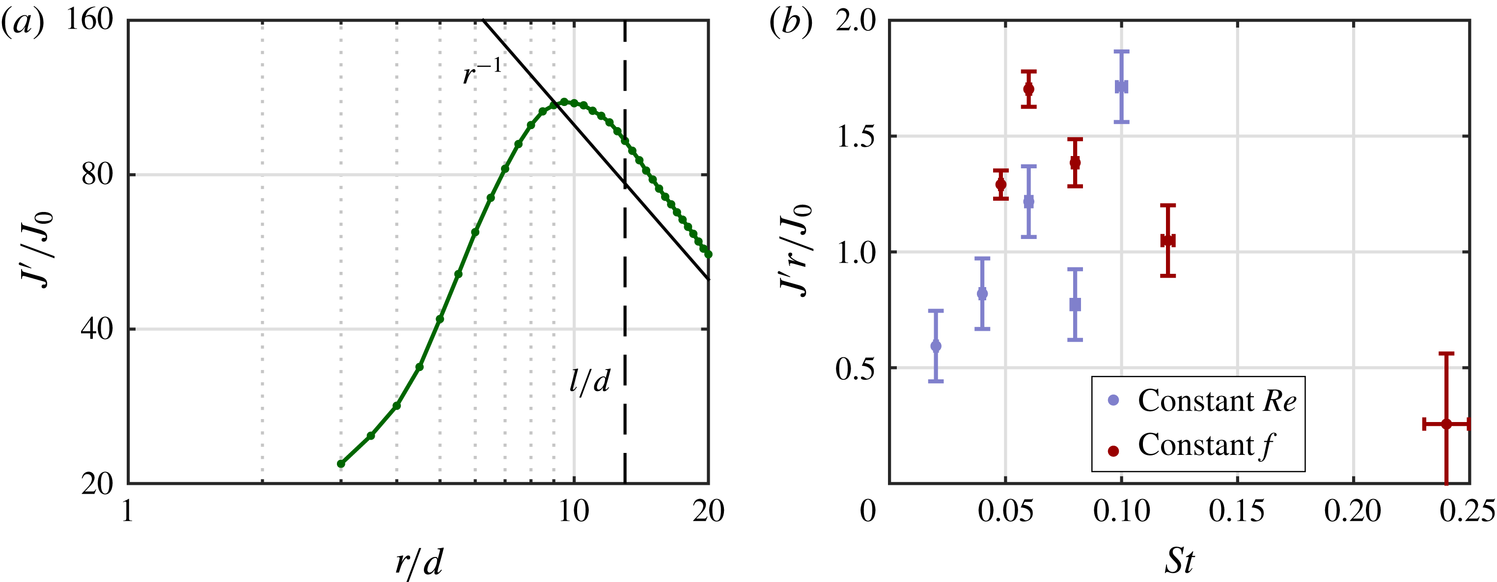
in figure 13(a). Representative for all cases, the momentum flux per unit depth decreases with approximately
 $r^{-1}$
for values of approximately
 $r/d>l/d$
(note that
 $l/d=AR=13$
), indicating a three-dimensional jet development in the far field. It was established in § 3.1.1 that the vortex trajectories and therefore the vectoring behaviour is governed by the near field and therefore assumed to be uninfluenced by this three-dimensional effect. Since only one plane is measured, the exact out-of-plane development of the jet is unknown. To account for the three-dimensional development, the momentum flux per unit depth is multiplied by the distance from the orifice,
 $r$
. This leads to a constant momentum flux,
 $J^{\prime }r$
(
 $\text{kg}~\text{m}~\text{s}^{-2}$
), related (but not equal) to the total momentum flux.
The uncertainty propagation of the velocity into the normalized quantity
 $J^{\prime }r/J_{0}$
scales with
 $1/\bar{u}$
and ranges from
 $\unicode[STIX]{x1D716}_{J^{\prime }r/J_{0}}=0.05{-}0.16$
.
3.2.1 Dependency of vectoring behaviour on Strouhal number
The included angle,
 $\unicode[STIX]{x0394}\unicode[STIX]{x1D6FD}$
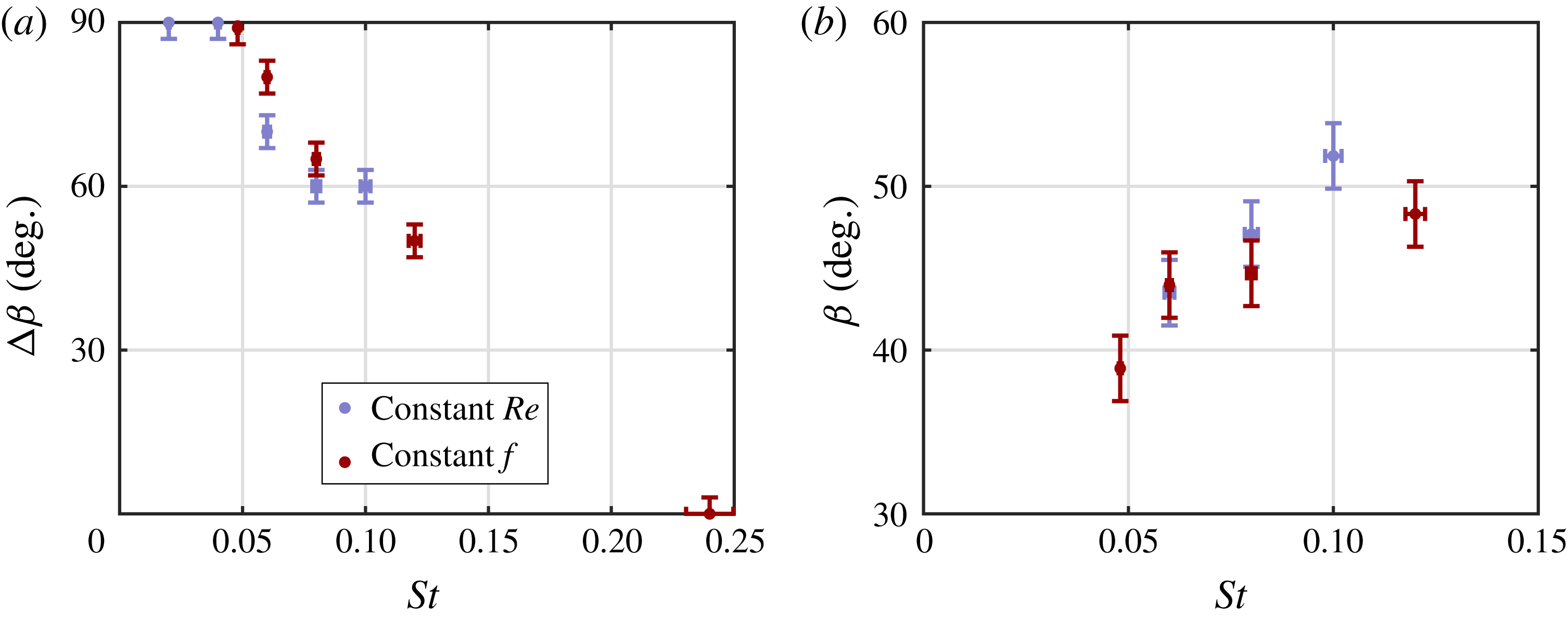
(degrees), is presented as function of the Strouhal number in figure 12(a). Note that for this quantitative analysis the Strouhal number and Reynolds number variations are lumped together. The included angle is
 $\unicode[STIX]{x0394}\unicode[STIX]{x1D6FD}=90^{\circ }$
up to approximately the formation number at
 $St\approx 0.05$
, after which it decreases. The included angle decreases relatively linearly with Strouhal number for all points that have a constant pinch-off time (i.e. all points in regime B as defined in figure 5).
The variation of vectoring angle with Strouhal number is plotted in figure 12(b). For clarity, the negative vectoring angles, corresponding to the cases in figures 6(a,b) and 9(h), are omitted. The vectoring angle shows an increasing trend with Strouhal number for the presented cases.
Included angle,
 $\unicode[STIX]{x0394}\unicode[STIX]{x1D6FD}$
(degrees), (a) and vectoring angle,
 $\unicode[STIX]{x1D6FD}$
(degrees), (b) as function of the Strouhal number for
 $\unicode[STIX]{x1D6E5}/d=2.0$
and
 $\unicode[STIX]{x1D703}=150^{\circ }$
. For clarity, outlier cases with negative vectoring angles as shown in figure 6 are omitted in (b).

Example of the variation of normalized momentum flux per unit depth,
 $J^{\prime }/J_{0}$
, with distance from the slot,
 $r/d$
, for
 $St=0.06$
,
 $Re=342$
,
 $\unicode[STIX]{x1D6E5}/d=2.0$
and
 $\unicode[STIX]{x1D703}=150$
degrees (a). Normalized momentum flux,
 $J^{\prime }r/J_{0}$
, as function of the Strouhal number for
 $\unicode[STIX]{x1D6E5}/d=2.0$
and
 $\unicode[STIX]{x1D703}=150^{\circ }$
(b).

The normalized momentum flux,
 $J^{\prime }r/J_{0}$
, is presented as function of the Strouhal number in figure 13(b). Up to
 $St=0.10$
, the normalized momentum flux increases with Strouhal number. This indicates that less of the momentum added by the actuators is ingested back into the actuators during the suction phase. For higher Strouhal numbers, the normalized momentum flux rapidly decreases, caused by the approach of the formation criterion.
3.2.2 Dependency of vectoring behaviour on phase difference and spacing
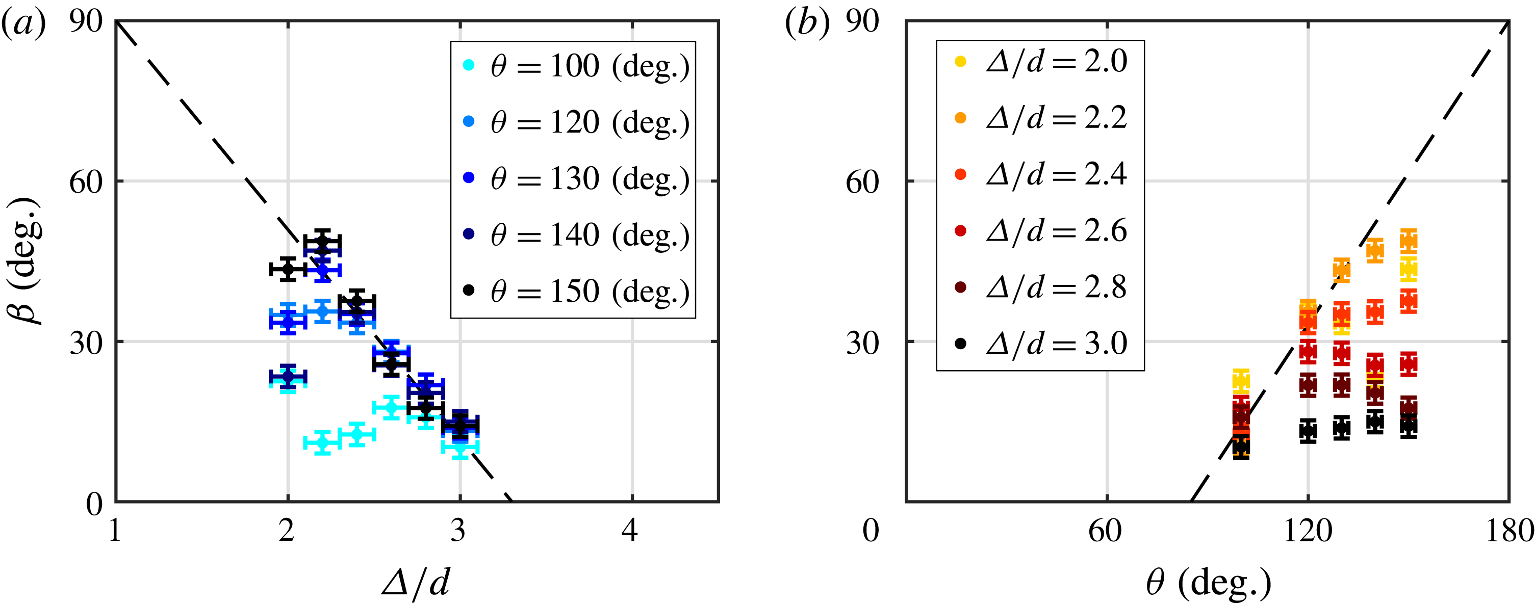
The variation of vectoring angle with phase difference and spacing is plotted in figure 14. The vectoring angle increases with phase difference up to a limit given by the spacing. The same pattern is observed for decreasing spacing, where the vectoring angle increases up to a limit given by the phase difference. This behaviour causes the variations to collapse onto two lines that suggest limiting behaviour. This collapse is indicated by the dashed lines in figure 14.
Vectoring angle,
 $\unicode[STIX]{x1D6FD}$
(degrees), as a function of (a) the spacing,
 $\unicode[STIX]{x1D6E5}/d$
, and (b) phase difference,
 $\unicode[STIX]{x1D703}$
(degrees), for
 $St=0.06$
and
 $Re=342$
.

The collapse of the vectoring angle onto these lines, and extrapolating those lines suggest that the maximum vectoring angle of 90 degrees (parallel to the plate) is reached at a phase difference of 180 degrees, which is the maximum possible phase difference and at a spacing of
 $\unicode[STIX]{x1D6E5}/d=1.0$
, which is the minimum possible spacing without overlapping the slots. This limiting behaviour is an interesting point of further study, where it must be noted that decreasing the spacing towards
 $\unicode[STIX]{x1D6E5}/d=1.0$
becomes increasingly hard since no material is present between the slots for this limit.
The lower limits of the vectoring angle indicate that vectoring does not occur at low phase differences, which is in agreement with the findings by Smith & Glezer (Reference Smith and Glezer2005) and neither at large spacings. It should be noted that Smith & Glezer (Reference Smith and Glezer2005) observed vectoring for a phase difference as small as 60 degrees and a spacing of
 $3.3d$
, which is beyond both limits shown in figure 14.
Normalized momentum flux
 $J^{\prime }r/J_{0}$
as a function of (a) the spacing,
 $\unicode[STIX]{x1D6E5}/d$
, and (b) phase difference,
 $\unicode[STIX]{x1D703}$
(degrees), for
 $St=0.06$
and
 $Re=342$
. See figure 14 for legend.

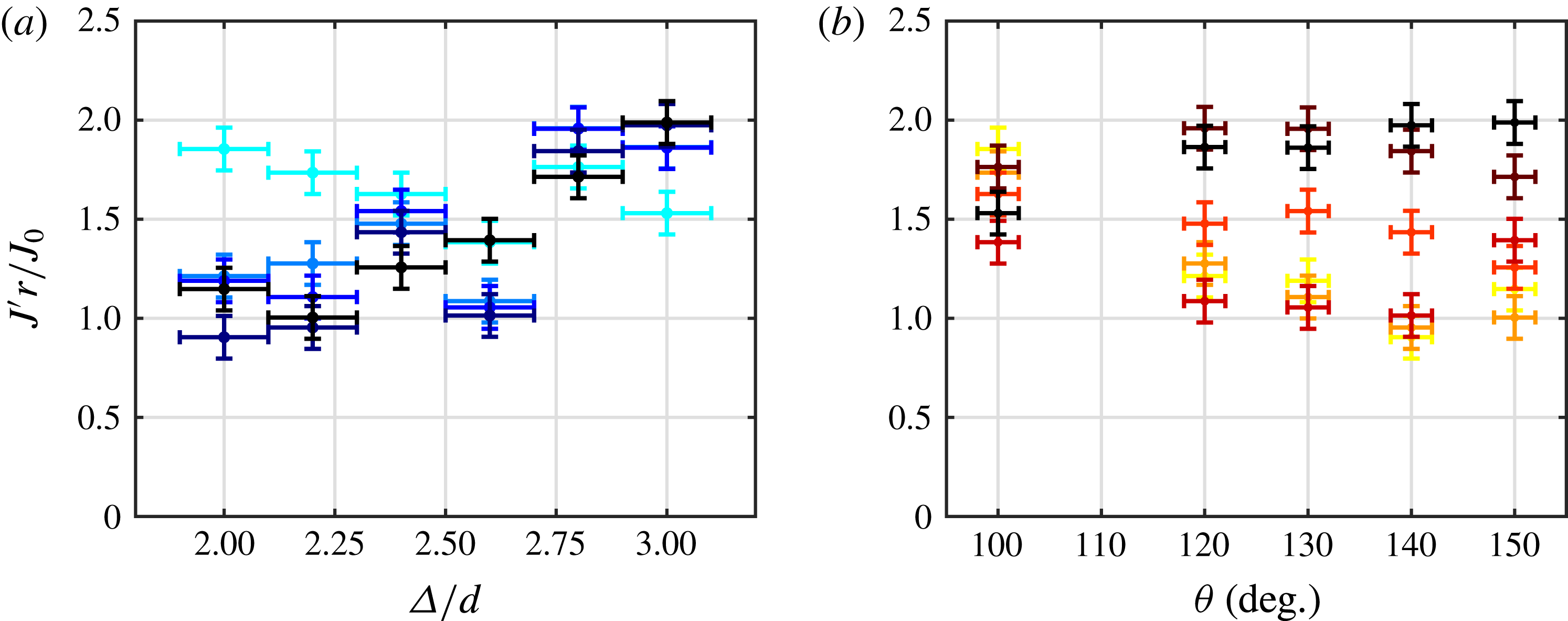
The variation of normalized momentum flux with phase difference and spacing is plotted in figure 15. The normalized momentum flux increases with spacing for all phase differences except
 $\unicode[STIX]{x1D703}=100$
degrees, for which it stays relatively constant. This increase is caused by less of the momentum of either jet being ingested into the neighbouring actuator. For
 $\unicode[STIX]{x1D703}=100$
degrees the influence of suction is less than for higher phase differences, as witnessed by the lower vectoring angles, causing ingestion of momentum to be absent and therefore invariant with spacing.
In a similar way, for small spacings the normalized momentum flux decreases for increasing phase difference, caused by more momentum being ingested into the neighbouring actuator. For larger spacings, ingestion of momentum is less prominent, causing less variation in the normalized momentum flux.
3.3 Physical mechanism describing vectoring behaviour
A physical mechanism that explains the variation in vectoring behaviour with the key parameters can be proposed based on the observations of the vortex trajectories obtained from phase-locked PIV data. This mechanism is valid for regime B as defined in figure 5 only where the vortex pinch off is at a fixed time (i.e.
 $t^{\prime }\approx 1/3$
). These vortex trajectories depend on the trade-off between the suction velocity of the actuator that is leading in phase, the induced velocity of the leading vortex pair and the distance between the vortex pairs from the lagging actuator and the leading actuator. Phase-locked vorticity maps for two cases with different Strouhal number are presented to demonstrate how the time-averaged vectoring behaviour can be reconciled based on the vortex trajectories that depend on the trade-off between the three contributions. This mechanism is then extended to include variations in Reynolds number, spacing and phase difference.
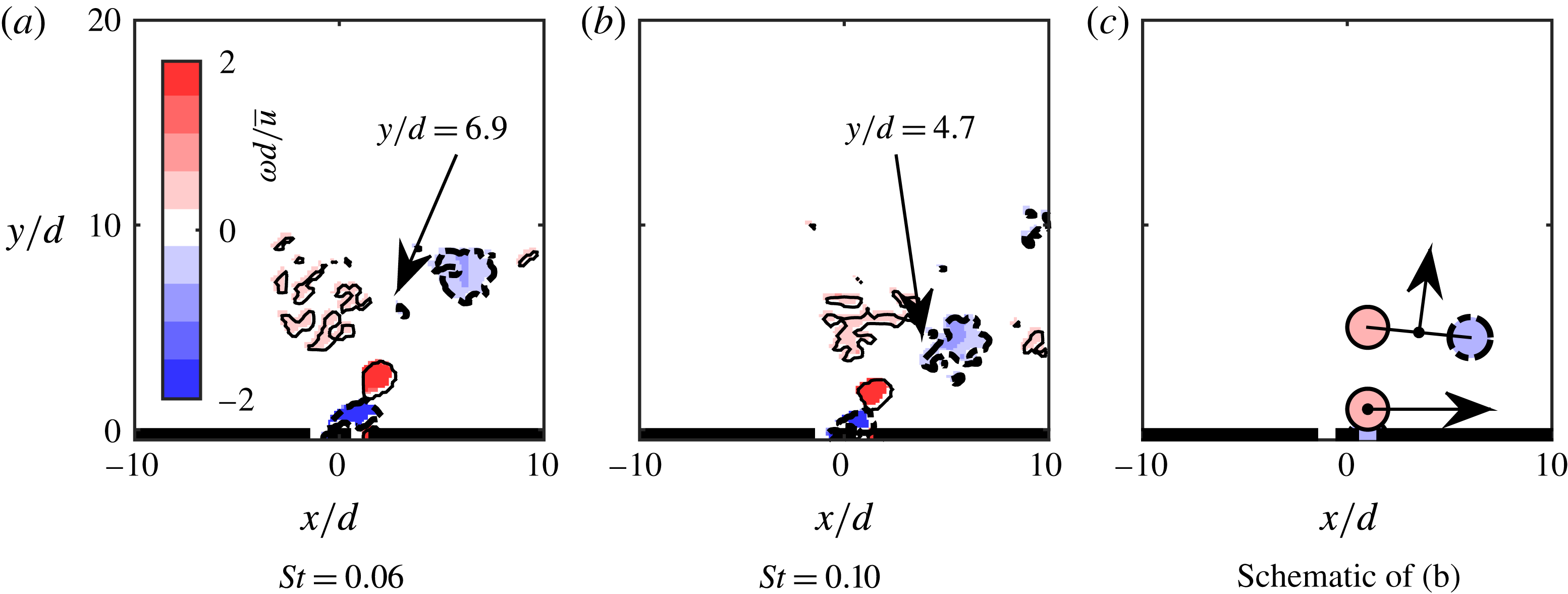
Phase-locked vorticity maps, showing vortex locations for
 $St=0.06$
(a) and
 $St=0.10$
(b), both for
 $Re=342$
,
 $\unicode[STIX]{x1D6E5}/d=2.0$
and
 $\unicode[STIX]{x1D703}=150$
degrees. The arrows in the schematic (c) indicate self-induced velocities of the vortex pair and the anticlockwise vortex. Red background with solid contour lines indicates positive vorticity, blue background with thick dashed contours indicates negative vorticity.

Phase-locked vorticity maps for
 $St=0.06$
and
 $St=0.10$
, with
 $Re=342$
,
 $\unicode[STIX]{x1D6E5}/d=2.0$
and
 $\unicode[STIX]{x1D703}=150$
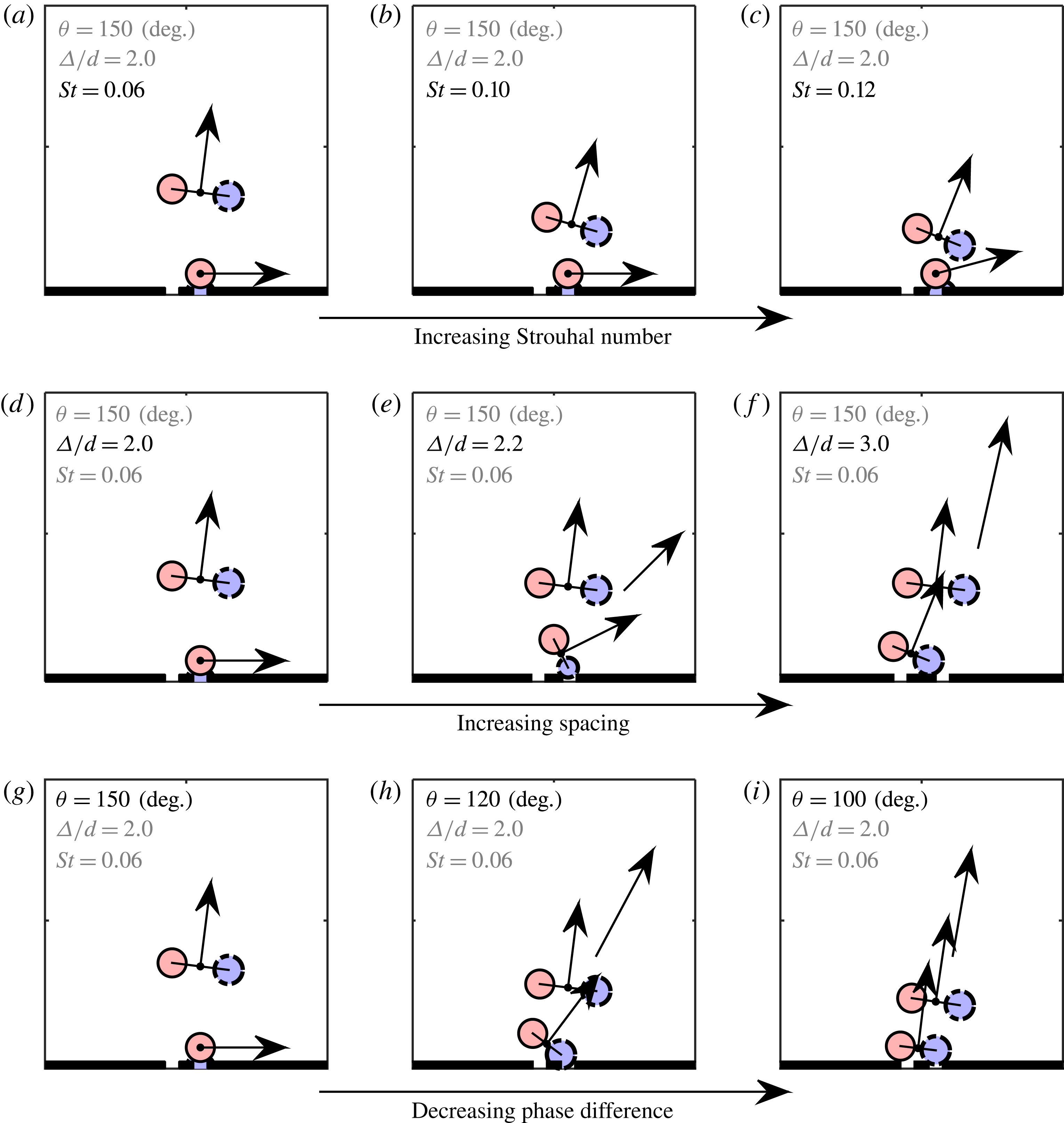
degrees are shown in figure 16(a,b). Vortex positions are identified using the swirling strength and the vorticity outside these positions is set to zero. Both cases are phase locked at the phase for which the clockwise rotating vortex produced by the actuator lagging in phase is about to be ingested into the leading actuator. In both cases, the vortex pair originating from the actuator leading in phase (actuator on the right) has propagated in the vertical direction. A schematic, representing the vortex positions in figure 16(b), is presented in figure 16(c) for clarity. The vortex pair has a self-induced velocity perpendicular to its axis, whereas the single anticlockwise vortex has a strong self-induced velocity towards the right, caused by the presence of its image vortex due to its vicinity to the surface. These self-induced velocities are indicated by the arrows in this schematic. The strong self-induced velocity of the single vortex prevents the branches from merging and creates a bifurcated jet. The Strouhal number (
 $St=0.10$
) corresponds to the case in figure 6(e) and indeed the arrows point in the direction of the bifurcated branches for this case.
The locations of the vortex pair centres in figure 16(a,b) are indicated by the arrow tips. The vertical positions (
 $y/d$
) of the leading vortex pairs are annotated in the graphs. The vortex pair originating from the actuator lagging in phase is influenced by the suction velocity of the actuator leading in phase, causing the vortex pair to rotate clockwise and move towards the right. The influence of the Strouhal number on the vertical location of the leading vortex pair can be considered using potential flow theory. During the formation of the vortices, the circulation,
 $\unicode[STIX]{x1D6E4}$
(
 $\text{m}^{2}~\text{s}^{-1}$
), grows as
 $\text{d}\unicode[STIX]{x1D6E4}/\text{d}t\approx u^{2}(t)/2$
(Shariff Reference Shariff1992). Assuming a jet velocity as given by (1.1) and a fixed pinch-off time (which is the case for regime B considered here), the circulation scales with
 $\unicode[STIX]{x1D6E4}\propto \bar{u}^{2}/f$
(note that
 $\unicode[STIX]{x1D6E4}\propto Re/St$
).
If the distance between the vortices within a vortex pair scales with the slot width (this is a reasonable assumption since the vortices are created at the edges of the slot), the self-induced velocity of the vortex pair scales as
 $u_{\unicode[STIX]{x1D6E4}}\propto \unicode[STIX]{x1D6E4}/d\propto \bar{u}^{2}/(fd)$
. The vertical position of the leading vortex pair,
 $y$
(m) will depend on the time since its creation (that varies as
 $\unicode[STIX]{x1D703}/f$
) and its self-induced velocity. Therefore, the vertical position will vary as
 $y/d\propto \unicode[STIX]{x1D703}/St^{2}$
. This inverse relation with the Strouhal number is evident in figure 16, where the vertical position of the centre of the leading vortex pair decreases from the
 $St=0.06$
to the
 $St=0.10$
case.
The closer proximity for the higher Strouhal number causes more interaction between the two vortex pairs. This leads to a decrease in the included angle between the two jets as presented in figure 12(a). The reduced vertical position (
 $y/d$
) of the leading vortex pair increases the induced velocity on the lagging vortex pair in the direction opposite to the suction velocity. This causes less of the lagging jet to be ingested into the leading actuator and thereby increases the normalized momentum flux as shown in figure 13(b). This increase in momentum flux mainly contributes to the horizontal momentum flux and thereby also increases the vectoring angle as shown in figure 12(b). The changes to the schematic in figure 16(c) for this variation with Strouhal number are presented in the schematics in figure 17(a–c), corresponding to the cases in figure 6(c,e,f).
Schematic representations of phase-locked vorticity maps, explaining the vectoring behaviour for the different parametric variations discussed in this study.

For the
 $St=0.12$
case, the distances from the single vortex to the leading vortex pair becomes close enough for the single vortex to be lifted away from the surface due to the velocity induced by the leading vortex pair as well as the low-pressure region in the wake of this pair. This causes the horizontal branch of the jet to become detached from the surface and shortly after its creation merge with the branch formed by the leading vortex pair, as is visible in the time-averaged flow field in figure 6(f).
A variation of Reynolds number can also be considered, starting from the same vortex positions as in figure 17(a). As discussed above, the vertical position of the leading vortex pair scales with
 $\unicode[STIX]{x1D703}/St^{2}$
, meaning that Reynolds number has no effect on the position of the vortices. However, the strength of the vortices, given by the circulation which scales as
 $Re/St$
, will be different. This change in vortex strength will be proportional for all the vortices, meaning that the interactions remain constant and therefore will not affect the vectoring behaviour. This is reflected in figure 9, where a change in Reynolds number does not lead to a significant change in the vectoring behaviour exhibited by the time-averaged flow field.
The above discussed physical mechanism based on vertical location of the vortex pair can also capture the influence of spacing. The vertical position of the leading vortex pair (scaling with
 $\unicode[STIX]{x1D703}/St^{2}$
) is invariant for changes in the spacing. However, increasing the spacing will cause the effect of the suction velocity on the lagging vortex pair to decrease. This is reflected in figure 17(d–f), corresponding to the cases in figure 10(a,d,j). Increasing the spacing to
 $\unicode[STIX]{x1D6E5}/d=2.2$
leads to the clockwise vortex of the lagging vortex pair not being completely ingested in the leading actuator. This means that there is no distinct horizontal branch originating from a single vortex above the surface and the branches will merge as is visible in figure 10(d). The large difference in orientation of the vortex pairs as indicated in figure 17(e) leads to a wide merged jet as in figure 10(d). Further increase in the spacing leads to less of the clockwise vortex being ingested into the leading actuator and a smaller rotation of the lagging vortex pair. For the
 $\unicode[STIX]{x1D6E5}/d=3.0$
case as presented in figure 17(f), no part of the clockwise vortex is ingested into the leading actuator and the lagging vortex pair is only slightly rotated. The lagging vortex pair is attracted by the low-pressure wake of the leading vortex pair, inducing a velocity on the lagging vortex pair towards the right. This will cause a wide merged jet, as visible in figure 10(j), but lowering the vectoring angle for increasing spacing as observed in figure 14(a).
Finally, the same physical description can be used to explain the behaviour with varying phase difference where both the vertical position of the leading vortex pair and the effect of suction are altered. Starting from the same baseline case (
 $St=0.06$
,
 $Re=342$
,
 $\unicode[STIX]{x1D6E5}/d=2.0$
and
 $\unicode[STIX]{x1D703}=150$
degrees), a decrease in phase difference is considered as presented in figure 17(g–i), corresponding to the cases in figure 10(a–c). Decreasing the phase difference to
 $\unicode[STIX]{x1D703}=120$
degrees decreases the vertical position of the leading vortex pair (scaling with
 $\unicode[STIX]{x1D703}/St^{2}$
) as presented in figure 17(h). In addition, the effect of suction on the lagging vortex pair decreases, leading to the clockwise vortex not being ingested into the leading actuator. Each vortex pairs is subjected to an induced velocity normal to its axis, while the lagging vortex pair is also attracted by the low-pressure wake of the leading vortex pair, leading to a merged jet vectored towards the leading actuator. Further decreasing the phase difference to
 $\unicode[STIX]{x1D703}=100$
degrees as presented in figure 17(i) diminishes the effect of suction on the lagging vortex pair. This implies that the vortex pairs are aligned and very close together. The lagging vortex pair is attracted by the low-pressure wake of the leading vortex pair, causing it to move slightly towards the leading actuator and merging with the leading vortex pair. This causes a compact merged jet, vectored towards the actuator leading in phase as observed in figure 10(c).
Although beyond the scope of the experiments in the present study, the influence of the aspect ratio on the presented two-dimensional mechanisms can be considered. A decrease in aspect ratio will increase three-dimensional effects not considered here. Ignoring these three-dimensional effects, the aspect ratio has another influence, as presented in (3.5). For increasing aspect ratio, the Strouhal number corresponding to the formation number (i.e. the dashed line in figure 5) will decrease. This means that regime B increases and more cases will pinch off at
 $t^{\prime }=1/3$
, but this will not change anything for the cases already in regime B as considered in the presented mechanism. For a decreasing aspect ratio this limiting Strouhal number will increase. This implies that cases in regime B might shift to regime A, thus pinching off sooner and therefore producing vortex pairs with less circulation. A decrease in circulation means that the effect of suction increases relative to the effect of self-induced velocity. Therefore, for a smaller aspect ratio, cases will bifurcate more easily and the cases in for example figure 17(e,h) might still lead to a bifurcated jet instead of a merged jet.
4 Conclusions
The vectoring of parallel synthetic jets can be described using five dimensionless parameters: the aspect ratio, Strouhal number, Reynolds number, spacing and phase difference. This study presents an experimental parametric study of the latter four, while using a fixed aspect ratio that we show to be large enough for the vectoring behaviour in the central plane of measurement to be dominated by a two-dimensional flow. Three regimes for the Strouhal number are defined. In the first regime the vectoring behaviour is dominated by the vortex pinch-off time. This study shows that – for a given actuator – the pinch-off time is a function of Strouhal number only. In the second Strouhal number regime the pinch-off time is invariant. A parametric study of all four parameters is performed inside this regime. In the third regime, no synthetic jet is formed due to the formation criterion.
For a small spacing (
 $\unicode[STIX]{x1D6E5}/d=2.0$
) and high phase difference (
 $\unicode[STIX]{x1D703}=150$
degrees) a bifurcated jet is formed with one vertical branch and one branch attached to the surface in the direction of the actuator leading in phase. It is shown that this bifurcation is the result of one of the vortices being ingested during the suction phase of the neighbouring actuator. For increasing Strouhal number the included angle between these branches decreases, while the total vectoring angle and the normalized momentum flux increase.
The variation of Reynolds number shows that (for multiple Strouhal numbers) a change in Reynolds number has negligible effect on both the included angle and the vectoring angle.
Increasing the spacing decreases the effect of suction on the neighbouring vortex pair. It is shown that for spacings larger than
 $\unicode[STIX]{x1D6E5}/d=2.0$
vortices are no longer ingested during the suction phase, cancelling bifurcation and leading to a wide merged jet. For increasing spacing, the vectoring angle becomes smaller, while the normalized momentum flux generally becomes larger.
Decreasing the phase difference also decreases the effect of suction on the neighbouring vortex pair. For phase differences lower than
 $\unicode[STIX]{x1D703}=150$
degrees, vortices are no longer ingested during the suction phase, cancelling bifurcation and leading to a compact merged jet. For a decreasing phase difference, the vectoring angle decreases and the normalized momentum flux either decreases (for small spacings) or is invariant (for larger spacings).
A physical mechanism – based on vortex locations at a single phase shortly after creation of the lagging vortex pair – is proposed that explains the vectoring behaviour for the full parameter space. This mechanism describes how some cases lead to ingestion of one of the vortices and bifurcation of the jet, while others do not. The relative location of the lagging vortex pair compared to the leading pair is used in the mechanism to describe the vectoring angle.
The results obtained in this research are relevant to flow control applications such as thrust vectoring and lay a groundwork for applications in which a cross-flow is present. The quantification of the variation of included angle, vectoring angle and momentum flux increases the level of control over the synthetic jets. The insights obtained in the present study can be used both in the design phase of a control system (e.g. jets with a specific spacing) as well as in the operational phase (e.g. actuating the jets with a specific Strouhal number, Reynolds number and phase difference).
Acknowledgements
We acknowledge the financial support from the European Research Council (ERC grant agreement no. 277472) and the Engineering and Physical Sciences Research Council (EPSRC grant no. EP/L006383/1). All data supporting this study are openly available from the University of Southampton repository at http://dx.doi.org/10.5258/SOTON/399446.
Supplementary movies
Supplementary movies are available at http://dx.doi.org/10.1017/jfm.2016.559.