
1. Introduction
Keeping a flow in the laminar state is a vital and a topical issue of interest for improving the performance of next-generation supersonic vehicles. Compared with turbulent flow, laminar flow is associated with lower skin friction drag, which can increase the efficiency of supersonic carriers and reduce emissions and the impact on the ozone. In addition, acoustic pollution to the ground is at a low level during take-off and landing when the flow is at laminar state. Therefore, it is important to control the onset of transition for supersonic boundary layers.
The transition will be initiated by the exponential growth of low-amplitude instability disturbances at a low level of background noise. Tollmien–Schlichting (TS) waves (Morkovin Reference Morkovin1983) are the most unstable instabilities in the incompressible boundary layer. For high-speed boundary layers, first-mode oblique waves are the most amplified instabilities for the supersonic boundary layer, while the hypersonic boundary layer is often dominated by the planar acoustic waves of the second mode (Mack Reference Mack1984). In the supersonic boundary layer, oblique-type breakdown is the most likely transition mechanism to initiate a transition in low-background-noise environments (Paredes, Choudhari & Li Reference Paredes, Choudhari and Li2017) compared with other transition scenarios, such as fundamental or subharmonic resonance (Corke & Mangano Reference Corke and Mangano1989; Franko & Lele Reference Franko and Lele2013) mechanisms initiated by a two-dimensional (2-D) wave and a pair of oblique waves. Fasel, Thumm & Bestek (Reference Fasel, Thumm and Bestek1993) found that a pair of oblique waves with equal frequency but opposite spanwise wavenumbers interact nonlinearly and can lead to a transition in the Mach 1.6 boundary layer with spatial direct numerical simulation (DNS). Subsequently, the nonlinear form of parabolized stability equations was considered by Chang & Malik (Reference Chang and Malik1994) to study the mechanism of oblique breakdown. They highlighted that the wave–vortex triad composed of the fundamental oblique waves and a streamwise vortex play an important role in the nonlinear stage of oblique breakdown. Higher harmonic waves are generated by the mutual interaction between the wave–vortex triad; when the amplitude of higher harmonic waves grows to the same order as the fundamental oblique waves, oblique breakdown is imminent. In addition, Chang & Malik (Reference Chang and Malik1994) indicated that the initial amplitude of oblique waves is lower than that of secondary instability mechanisms to trigger the transition of the boundary layer. Leib & Lee (Reference Leib and Lee1995) provided a theoretical basis for the oblique breakdown mechanism by Reynolds number asymptotic theory, and they proved that the explosive growth of oblique waves is a generic feature of oblique breakdown. Kosinov, Semionov & Shevelkov (Reference Kosinov, Semionov and Shevelkov1994) and Kosinov, Maslov & Semionov (Reference Kosinov, Maslov and Semionov1997) conducted a series of experiments at a supersonic boundary layer. However, they focused on a mechanism called asymmetric subharmonic resonance, not oblique breakdown. Fezer & Kloker (Reference Fezer and Kloker2000) have, however, shown that the oblique breakdown does play the dominant role in the scenario, but can be enriched by the asymmetric subharmonic resonance. Subsequently, a series of DNSs (Jiang et al. Reference Jiang, Choudhari, Chang and Liu2006; Mayer, Wernz & Fasel Reference Mayer, Wernz and Fasel2011a; Mayer, Von Terzi & Fasel Reference Mayer, Von Terzi and Fasel2011b; Franko & Lele Reference Franko and Lele2013; Mayer et al. Reference Mayer, Fasel, Choudhari and Chang2014) were conducted to address two issues. First, they proved that there is not only asymmetric subharmonic resonance but also oblique breakdown in the experiments of Kosinov et al. (Reference Kosinov, Semionov and Shevelkov1994, Reference Kosinov, Maslov and Semionov1997). Second, they found that oblique breakdown was able to lead to a fully developed turbulent flow. Recently, Laible & Fasel (Reference Laible and Fasel2016) found that the transient growth mechanism played a significant role in converting the stationary vortex mode into streamwise streaks, and the instability of streaks would ultimately cause laminar breakdown.
With the understanding of the oblique breakdown mechanism, streaks have been used to control the transition. Compared with active control, passive control does not rely on complicated sensitive sensor–actuator systems. Streaks involving high and low streamwise velocities have been proven to be an efficient laminar technique. A series of experimental and theoretical studies (Cossu & Brandt Reference Cossu and Brandt2002; Fransson et al. Reference Fransson, Brandt, Talamelli and Cossu2005; Bagheri & Hanifi Reference Bagheri and Hanifi2007) showed that streaks can reduce the growth rate of TS waves. Fransson et al. (Reference Fransson, Talamelli, Brandt and Cossu2006) and Shahinfar et al. (Reference Shahinfar, Sattarzadeh, Fransson and Talamelli2012) successfully controlled the TS wave in an incompressible boundary layer though roughness along the body surface to induce steady streamwise streaks. However, the amplitude of the streaks should be lower to avoid shear layer instabilities. For oblique breakdown in the high-speed boundary layer, streaks do not seem to effectively delay the transition because of their inherent streak modes. Moreover, limited experimental studies (Holloway & Sterrett Reference Holloway and Sterrett1964) have investigated roughness-induced streaks in high-speed boundaries, and the streaks have been found to be highly dependent on the shape, height and spacing of roughness. Recently, Paredes et al. (Reference Paredes, Choudhari and Li2017) investigated the interaction between oblique first-mode waves and streaks generated by the transient growth of an optimal initial perturbation with nonlinear plane-marching parabolized stability equations. They concluded that the spanwise wavenumbers of the streaks must be at least two times greater than the oblique waves with the most growth. Subsequently, Sharma et al. (Reference Sharma, Shadloo, Hadjadj and Kloker2019b) conducted DNSs to study the delay effect of streaks on oblique breakdown. They found that streaks with spanwise wavenumbers four to five times those of the fundamental oblique waves have effective control effects, and streaks with higher spanwise wavenumbers have faster streak decay in the streamwise direction. Then Kneer, Guo & Kloker (Reference Kneer, Guo and Kloker2022) employed streaks to control oblique breakdown, subharmonic combination-resonance triad and point source successfully in a supersonic boundary layer. It should be noted that, except for steady mode (0,2), steady modes with higher spanwise wavenumbers will also be generated during the nonlinear stage of oblique breakdown, which satisfies the spanwise wavenumbers being at least two times greater than the fundamental oblique waves. Can we use those higher spanwise wavenumber steady modes generated at the nonlinear stage of oblique breakdown to suppress the growth of fundamental oblique waves?
Local cooling or heating can be considered a technique for laminar flow control based on the stabilization effect of cooling walls on the first-mode disturbances or the stabilization effect of heating walls on the second-mode disturbances (Mack Reference Mack1984). Masad & Abid (Reference Masad and Abid1995) found that both stabilization and destabilization of the supersonic boundary layer caused by the local heating strip are possible depending mainly on the position of the heating strip. Subsequently, the wall temperature jump effect was studied numerically and theoretically (Inger & Gnoffo Reference Inger and Gnoffo2001) in supersonic laminar flow, and they provided an efficient tool for the calculating of local heat transfer. Soudakov, Egorov & Fedorov (Reference Soudakov, Egorov and Fedorov2009) conducted a 2-D DNS on a flat boundary layer. It was concluded that compression waves are induced from cold to hot walls and make the boundary layer thicker. In contrast, expansion waves are induced from hot to cold walls and lead to a thinner boundary layer. Moreover, the temperature jump will affect the stability of the boundary layer. Recently, several numerical studies (Fedorov et al. Reference Fedorov, Soudakov, Egorov, Sidorenko, Gromyko, Bountin, Polivanov and Maslov2015; Oz & Kara Reference Oz and Kara2021) have been conducted to investigate the effect of local cooling on the stability of a high-speed boundary layer. They found that localized cooling can decrease the second-mode amplitude and that the effectiveness of local cooling is higher than that of full cooling. Zhao et al. (Reference Zhao, Wen, Tian, Long and Yuan2018) indicated that the synchronization point significantly affects the stability of the slow mode. The above studies focus on the effect of local cooling or heating on the stability of the boundary layer or study the transition onset affected by local heating or cooling through N-factors, which are solved by linear stability theory. However, it is known that there are many strong nonlinear interaction involved in the transition process, and limited research has studied the effect of local cooling or heating on the specific transition path. Recently, Jahanbakhshi & Zaki (Reference Jahanbakhshi and Zaki2021) successfully employed an optimal steady wall heat flux to delay the breakdown of most dangerous disturbances in a supersonic boundary layer. Subsequently, three-dimensional (3-D) DNSs (Zhou et al. Reference Zhou, Lu, Liu and Yan2021) were conducted to study the control effect of cooling strips on oblique breakdown in a supersonic boundary layer. They found that the location of the cooling strip has a great effect on the transition onset of oblique breakdown. The cooling strip can delay the transition, causing it to occur more downstream with a temperature decrease. In addition, the cooling strip in the proper streamwise region could induce the stabilization effect of the higher spanwise wavenumbers generated during the nonlinear stages of oblique breakdown on suppressing the growth of fundamental oblique waves and cause breakdown far downstream, which is called the self-suppression effect (SSE) in the present study. It should be noted that the local cooling strip embedded in the adiabatic wall was employed in their studies with no temperature jump downstream of the cooling strip, which means that the cooling temperature is lower and that the longer wall downstream of the cooling strip will be cooled. Even a narrow cooling strip with a low cooling temperature can prevent oblique breakdown, as a long wall downstream of the cooling strip will be cooled due to the adiabatic wall boundary condition (see figure 1). Additionally, only one SSE occurs in the study of Zhou et al. (Reference Zhou, Lu, Liu and Yan2021), and the requirements for the SSE are not given.
Effect of the wall boundary condition on the distribution of the wall temperature downstream of the cooling strip. The solid and dashed lines represent the wall temperature distribution of isothermal and adiabatic walls, respectively.

Thus, the main objective of this paper is to study the control effect of cooling strips embedded in an isothermal wall on oblique breakdown in a supersonic boundary layer using DNSs, which will include a temperature jump downstream of the cooling strip and is in line with real situations. Some questions need to be addressed. First, how do transition onsets change with temperature variation? With the temperature jump downstream of the cooling strip, is the transition onset still changing monotonically with temperature as in Zhou et al. (Reference Zhou, Lu, Liu and Yan2021), or will it be reversed? Moreover, are SSEs still present to make the oblique breakdown occur farther downstream? What requirements are taken to trigger the SSE? How many times can the SSE occur in one test case?
The paper is organized as follows. Section 2.1 provides a description of the computational set-up in this study. Details of the DNS solver, boundary condition and cooling profile are presented in §§ 2.2, 2.3 and 2.4, respectively. Then, validation studies are conducted in § 2.5. The results are shown in § 3. First, the effect of temperature on the stability of the initial oblique wave is studied by linear stability theory (LST) in § 3.1, followed by the transition onset solved by DNS with different criteria in § 3.2. Subsequently, the transition onset differences will be explained in §§ 3.3, 3.4, 3.5 and 3.6, including the SSE, transition reverse and effect of cooling width and soften cooling edge. Finally, conclusions are presented in § 4.
2. Computation set-up and validation
The purpose of the present study is to investigate the control effect of local cooling strips on oblique breakdown in a supersonic boundary layer with Mach number  $M_\infty =2.0$ using spatial DNS. The simulation set-up is designed to allow comparisons and match the flow conditions with Fezer & Kloker (Reference Fezer and Kloker2000) or Sharma et al. (Reference Sharma, Shadloo, Hadjadj and Kloker2019b). The details of the free stream conditions are shown in table 1. Here
 $Ma$,
 $T$,
 $Re$,
 $\gamma$,
 $Pr$,
 $u$ and
 $L_{ref}$ are the Mach number, temperature, Reynolds number, heat capacity ratio, Prandtl number, streamwise velocity and reference length, respectively. Subscripts
 $w$ and
 $\infty$ denote the flow parameters of the wall and free stream, respectively. The Sutherland law with no low-temperature correction was employed to calculated the viscosity.
Free stream flow condition.

2.1. Computation set-up
Figure 2 denotes the simulation set-up for all cases. To capture the turbulence region of different cases, two computational domains with different lengths in the streamwise direction and the same width in the spanwise and wall-normal directions are employed. The inflow is set at  $x_{in}=4.154\ \mathrm {mm}$ (
 $Re_x=1.0\times 10^{5}$), where
 $Re_x=Re\,x$. The boundary layer thickness at the inflow of the domain is
 $\delta _{in}=8.528\times 10^{-2} \mathrm {mm}$. The lengths of the two computational domains in the streamwise direction are
 $L_x=55 \ \mathrm {mm}$ (from
 $Re_x=1.0\times 10^{5}$ to
 $14.2\times 10^{5}$) and
 $75 \ \mathrm {mm}$ (from
 $Re_x=1.0\times 10^{5}$ to
 $19.0\times 10^{5}$). At the end of the domain, a sponge region is utilized to dissipate disturbance reflection from the outlet boundary. The length of this sponge region is
 $x_{sponge} \approx 120\delta _{in}$. The width and height of the domain are
 $L_z=2.153\ \mathrm {mm}$ (
 $L_z/\delta _{in}=25.2$) and
 $L_y=5.1\ \mathrm {mm}$ (
 $L_y/\delta _{in}=59.8$), respectively. For the longer computational domain, the height of the computational domain is approximately 13.7 times the boundary layer thickness (laminar) at the outflow.
Schematic of the computational domain and boundary conditions.

Equidistant grid spacing is applied in the streamwise ( $x$) and spanwise (
 $z$) directions. Grid stretching is employed in the wall-normal (
 $y$) direction, which is shown in figure 3. The numbers of grids in the three directions
 $n_x\times n_y \times n_z$ for two different domains are
 $3030 \times 156 \times 160$ and
 $4120 \times 156 \times 160$, respectively. The grid resolution for the cases in the present study is
 $\Delta x^{+}_{max} \times \Delta y^{+}_{w} \times \Delta z^{+}_{max} = 9.04 \times 0.78 \times 6.64$, which is defined as
 $\Delta x^{+}_i= \sqrt {(\tau _w \rho _w)}\Delta x_i/\mu _w$, where
 $\tau _w$ represents the wall shear stress at the stream position where the skin-friction coefficient reaches the maximal value.
The distributions of grid points in the wall-normal direction. (a) Every three points in the  $y$ direction and 10 points in the
 $x$ direction are shown and (b) grid stretching in the wall-normal direction.

2.2. Numerical method
The governing equations are the non-dimensionalization form of unsteady compressible Navier–Stokes (N–S) equations,
 \begin{equation} \frac{\partial \boldsymbol{Q}}{\partial t}+\frac{\partial \boldsymbol{F}_{c,j}}{\partial x_j}=\frac{1}{Re} \frac{\partial \boldsymbol{F}_{v,j}}{\partial x_j}, \quad (\kern0.06em j=1,2,3), \end{equation}
where
 \begin{align} \boldsymbol{Q} = \left(
\begin{array}{@{}c@{}} \rho \\ \rho u_i \\ \rho e \end{array}
\right), \quad \boldsymbol{F}_{c,j} = \left(
\begin{array}{@{}c@{}} \rho u_j \\ \rho u_iu_j + p\delta_{ij} \\
(\rho e+p)u_j \end{array} \right), \quad
\boldsymbol{F}_{v,j} = \left( \begin{array}{@{}c@{}} 0 \\
\sigma_{ij} \\ \sigma_{ij}u_i+q_j \end{array} \right),\quad
(i,j=1,2,3) \end{align}
are conservative variables, convective flux vectors and viscous flux vectors, respectively. Here  $\delta _{ij}$ represents the Kronecker delta, and
 $u$ is the velocity vector. The total energy
 $e$, the viscous stress tensor
 $\sigma _{ij}$, and the heat flux
 $q_i$ can be calculated as
 \begin{align}
e=\frac{p}{(\gamma-1)\rho}+\frac{u^{2}_i}{2},\quad
\sigma_{ij}=\left\{ \begin{array}{@{}ll} \mu \left(
\dfrac{\partial u_j}{\partial x_i}+\dfrac{\partial
u_i}{\partial x_j}\right), & i\not= j, \\
2\mu\dfrac{\partial u_i}{\partial x_i}-\dfrac{2}{3}\mu
\boldsymbol{\nabla}\boldsymbol{\cdot}\boldsymbol{u}, &
i=j, \end{array} \right.\quad q_i=k\frac{\partial
T}{\partial x_j}, \end{align}
respectively, where  $k$ is the thermal conductivity. Assuming the fluid to be a perfect gas, (2.1) can be closed by the state equation
 \begin{equation} p=\frac{\gamma-1}{\gamma}\rho T. \end{equation}
The DNS code OpenCFD developed by Li, Fu & Ma (Reference Li, Fu and Ma2010a) is employed to solve the governing equations. The governing equations are solved in non-dimensional form where the length, velocity components, density, temperature and pressure are non-dimensionalized by the length scale  $L_{ref}$, streamwise velocity
 $u_\infty$, density
 $\rho _\infty$, temperature
 $T_\infty$ and pressure scale
 $\rho _\infty u^{2}_\infty$, respectively; the subscript
 $\infty$ represents free stream. In addition, the Reynolds number is defined as
 $Re=\rho _\infty u_\infty L_{ref}/\mu _\infty$. This parallel DNS solver has been validated to be reliable by using previous studies (Li et al. Reference Li, Fu, Ma and Liang2010b, Reference Li, Tong, Yu and Li2019). An optimized sixth-order monotonicity-preserving scheme (Li, Leng & He Reference Li, Leng and He2013) with Steger–Warming splitting (Steger & Warming Reference Steger and Warming1981) is used for the spatial discretization of the convective terms. A sixth-order central difference scheme is used for the computation of the viscous terms. A third-order total-variation-diminishing-type Runge–Kutta method (Jiang & Shu Reference Jiang and Shu1996) is employed for time advancement.
2.3. Boundary conditions
The boundary conditions utilized in this study are shown in figure 2. At the inlet of the computational domain, supersonic inflow boundary conditions are used. All of the flow variables at the inlet are solved by compressible Blasius equations (Stewartson Reference Stewartson1964) with the shooting method. To validate the inlet boundary condition, a comparison with the solution of 2-D N–S equations is presented in figure 4. To get the solution of 2-D N–S, a 2-D laminar flat-plate boundary layer including the leading edge is simulated with the same numerical methods as the DNS. The inlet of the plate is set to free stream. At the bottom of computation domain, symmetric boundary conditions are applied upstream of the leading edge, and a no-slip isothermal wall is employed downstream of the leading edge. Then, the solution of 2-D N–S is found at streamwise station  $x=0.004154$ m. Good agreement is observed, except for the slight differences of temperature profiles above the edge of boundary layer, as the shock induced by the leading edge of the plate wave will be involved in 2-D N–S. A non-reflecting boundary condition is utilized for the upper boundary layer. Periodic conditions and supersonic outlet boundary conditions are used for two lateral boundaries and the outlet of the domain, respectively. The wall of the domain is set to be a non-slip isothermal wall with boundary condition
 $\partial p/\partial n=0$. Except for the local cooling strip, the temperature of the wall is
 $T_w=1.67T_\infty$, which is very close the temperature of the adiabatic wall for laminar flow estimated with a recovery factor of
 $r=Pr^{1/2}$ (White Reference White2006):
 \begin{equation} T_{aw}=T_{\infty}\left(1+r\frac{\gamma-1}{2}Ma^{2}_\infty\right). \end{equation}
Within the local cooling strips, the wall temperature is set to  $T=0.75T_w$,
 $T=0.50T_w$ and
 $T=0.25T_w$ for different cases.
Validation of flow variable profiles employed as the inlet boundary condition: (a) streamwise velocity  $u$ and (b) temperature
 $T$.

The oblique waves are initialized by a wall blowing and suction strip (Sharma et al. Reference Sharma, Shadloo, Hadjadj and Kloker2019b), which can be described as
 \begin{equation} \rho v(x,y=0,z,t)=A\rho_{\infty}u_{\infty}f(x)g(z)h_1(t), \end{equation}
where
 \begin{gather} f(x)=\frac{4}{\sqrt{27}}\sin\theta(1-\cos\theta),\quad \theta=2{\rm \pi}\frac{x-x_{start}}{x_{end}-x_{start}}, \end{gather}
 \begin{gather} g(z)=({-}1)^{k}\cos(k\beta_{0}z), \quad h_1(t)=\sin(2{\rm \pi} hf_{0}t), \end{gather}
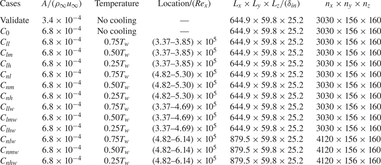
where  $A$ is the forcing amplitude, whose values for all cases are shown in table 2. The blowing and suction strip extends from
 $x_{start}=8.308\ \mathrm {mm}$ (
 $Re_x=2.0\times 10^{5}$) to
 $x_{end}=13.808\ \mathrm {mm}$ (
 $Re_x=3.32\times 10^{5}$). The fundamental frequency and spanwise wavenumber are set to
 $f_0=73.83\ \mathrm {kHz}$ and
 $\beta _0=2{\rm \pi} /\lambda _z=2.9176\ \mathrm {mm^{-1}}$, respectively. The spanwise wavelength is equal to the spanwise width of the computational domain (
 $\lambda _z=L_z=2.153\ \mathrm {mm}$). The pair
 $(h, k)$ denotes the sum of modes with frequency
 $h\omega _0$ and spanwise wavenumber
 ${\pm }k\beta _0$ in the following.
Details of all of the cases in this study. The naming scheme is composed of three or four characters: the first character is ‘C’, followed by two or three characters as subscripts. The first subscript being  $l$ or
 $n$ represents the cooling strip being employed at the linear or early nonlinear region of oblique breakdown, respectively; see figure 9. The second subscript options,
 $l$,
 $m$ and
 $h$, are used to describe the cooling strips with ‘low cooling’
 $T=0.75T_w$, ‘medium cooling’
 $T=0.50T_w$ and ‘highly cooling’
 $T=0.25T_w$ characteristics, respectively. The last subscript
 $w$ represents a cooling strip with a wider width, which is equal to the width of a blowing and suction strip; the absence of
 $w$ means the width of the cooling strip is narrow, i.e. four-elevenths of the wider width.

2.4. Cooling profile set-up
The wall temperature jump along an isothermal wall is a fundamental problem arising in the thermal protection system as the presence of different wall materials (Inger & Gnoffo Reference Inger and Gnoffo2001). Thus, the flat cooling profile (Oz & Kara Reference Oz and Kara2021) with the temperature jump at the edge of cooling strip is employed for most cases in present study (see figure 5, for comparison). To keep the integral of cooling temperature minus the wall temperature over the cooling area the same as the flat cooling profile, a linear soften edge is used. The linear soften edge with  $b=1\ \mathrm {mm}$ is only set for case
 $C_{nh}$ to study the influence of the cooling profile on the transition onset (see § 3.6).
The cooling profile used in the present study. The solid and dashed lines represent the flat cooling profile and flat cooling profile with linear soften edge, respectively. Here  $s$ is the width of cooling strip and
 $b$ is the soften width.

2.5. Validation
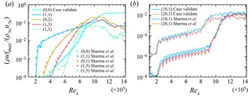
First, we validate the streamwise evolution of various modes solved by our DNS solver. Each mode is computed by a fast Fourier transform in both the time and spanwise directions. Then, the maximum value is chosen in the wall-normal direction. Time sampling is conducted over two fundamental periods with sampling frequency  $16.88\ \mathrm {MHz}$. The forcing amplitudes for case ‘validate’ are different from those in Sharma et al. (Reference Sharma, Shadloo, Hadjadj and Kloker2019b) by a factor of two. This difference can also be seen in Kneer (Reference Kneer2020), which might be caused by normalization. It is noted that an adiabatic wall is employed in Sharma et al. (Reference Sharma, Shadloo, Hadjadj and Kloker2019b). An isothermal wall with temperature
 $T_w=1.67T_{\infty }$, which is very close to the adiabatic wall, is utilized in our study. Good agreement is observed between the current results and Sharma in figure 6(a). Differences can be seen for higher wavenumber modes at low amplitudes, indicating that the background noise in our solver is lower than that in Sharma et al. (Reference Sharma, Shadloo, Hadjadj and Kloker2019b). The initial noise caused by our solver is approximately
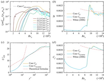
 $10^{-8}$, which is two orders of magnitude smaller than that in Sharma et al. (Reference Sharma, Shadloo, Hadjadj and Kloker2019b) (see figure 6b). A brief summary of the wall resolution of some DNS studies of high-speed transitional and turbulent boundary layer flows is shown in table 3. Then, grid sensitivity studies are conducted to validate the grid resolution (see Appendix A).
Comparison of modal disturbance development in the streamwise direction with case Cref in Sharma et al. (Reference Sharma, Shadloo, Hadjadj and Kloker2019b). (a) Evolution of the main modal disturbances and (b) high-frequency modes generated from the solver.

Summary of DNSs of the transition in the supersonic boundary layer. References: Pirozzili et al. (2004); Li et al. (2009); Mayer et al. (2011); Sharma et al. (2019).

3. Results
3.1. Linear stability analysis
In this section, LST is employed to study the effect of wall temperature on the stability of the initial disturbance. The LST code validation is given in Appendix B. For a given streamwise station, frequency  $f$ and spanwise wavenumber
 $\beta$, the complex streamwise wavenumber
 $\alpha =\alpha _r+{\rm i}\alpha _i$ can be solved by the LST solver. For the positive values of
 $\alpha _i$, the amplitude of this disturbance is damped in the streamwise direction, whereas negative values indicate amplification.
The LST is utilized to address two questions. The first is that the frequency and spanwise wavenumber of fundamental oblique waves are the same as Sharma et al. (Reference Sharma, Shadloo, Hadjadj and Kloker2019b), but we change the adiabatic wall to an isothermal wall. Thus, we use LST to analyse the stability of the fundamental oblique waves and study the effect of temperature on the amplification rate of the fundamental oblique waves. The second question is whether the lowest temperature ( $T=0.25T_w$) used in this study will lead to the second mode, as the cooling wall might lead to unstable second modes (Lysenko & Maslov Reference Lysenko and Maslov1984).
We track the streamwise evolution of discrete mode F and mode S of 2-D waves with  $f=73.83\ \mathrm {kHz}$ and
 $\beta =0$ for different wall temperatures (see figure 7a). For
 $x\rightarrow 0$, the phase velocities of mode S and mode F synchronize with the slow acoustic wave spectrum (
 $c_r=1-1/Ma=0.5$) and fast acoustic wave spectrum (
 $c_r=1+1/Ma=1.5$), respectively. When the phase velocities of both discrete modes coincide at a synchronism point, mode S is usually responsible for second-mode instability (Fedorov & Khokhlov Reference Fedorov and Khokhlov2002). However, the phase velocity evolution of both discrete modes in the streamwise direction is very close to the acoustic wave spectrum, even at more downstream streamwise stations than the end of the longer computational domain (vertical dashed line). Thus, the lowest temperature (
 $T=0.25T_w$) cannot lead to the second mode in our computational domain.
(a) Evolution of phase velocity  $c_r$ of modes F and S with different wall temperatures in the streamwise direction for 2-D disturbances with
 $f=73.83\ \mathrm {kHz}$. Vertical dashed and horizontal dashed dotted lines indicate the end of the longer computational domain and the phase velocity of the slow acoustic wave spectrum, respectively. (b) Evolution of
 $\alpha _i$ in the streamwise direction for different wall temperatures, solid and dashed lines for 2-D disturbances with
 $f=73.83\ \mathrm {kHz}$ and 3-D disturbances with
 $f=73.83\ \mathrm {kHz}$ and
 $\lambda _z=2.153\ \mathrm {mm}$, respectively.

The effect of temperature on the stability of 2-D and 3-D disturbances is denoted in figure 7(b). When the wall temperature is set to  $T=T_w$, there is a first-mode region for both 3-D and 2-D disturbances. The unstable region of 3-D disturbance is larger than that of 2-D disturbance. When the wall temperature is cooled, all the disturbances are damped. The temperature is lower and the disturbances are damped more quickly, which is consistent with Malik (Reference Malik1989) and Mack (Reference Mack1984).
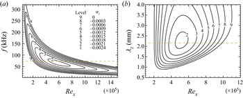
The contour levels of  $\alpha _i$ are plotted at a spanwise wavelength of interest,
 $\lambda _z=2.153~\mathrm {mm}$, with different frequencies at different streamwise positions (see figure 8a). Figure 8(b) shows at a constant frequency of interest,
 $f=73.83~\mathrm {kHz}$. The results in both figures indicate that the fundamental oblique instability wave used in the DNS has a high amplification rate at
 $Re_x\approx 5.0\times 10^{5}$. Although the unstable region for the initial oblique wave cannot cover the whole computation domain, it is sufficiently long to actuate nonlinear interaction between various modes and trigger oblique breakdown (see figure 27). It should be noted that the flow is assumed to be parallel in the LST, but the local cooling strip will make the boundary layer more non-parallel. Furthermore, oblique breakdown is mainly a nonlinear process, but the LST is suitable for linear analysis. Additionally, a temperature jump is involved at the end of the cooling strip. Therefore, we will give the results solved by DNS and show more high-fidelity flow details in the following sections.
Contours of  $\alpha _i$ solved by LST: (a) for constant spanwise wavelength
 $\lambda _z=2.153\ \mathrm {mm}$; (b) for a constant frequency
 $f=73.83\ \mathrm {kHz}$. The dashed lines indicate the frequency (
 $\,f=73.83\ \mathrm {kHz}$) and spanwise wavelength (
 $\lambda _z=2.153\ \mathrm {mm}$) of interest.

3.2. Onset of transition
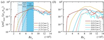
The oblique breakdown is divided into linear, early nonlinear and late nonlinear stages (see figure 9a). The linear stage of oblique breakdown is dominated by mode (1,1), but there is no definition of the boundary between the linear and early nonlinear stage. We define the end of the linear stage at where the amplitude of mode (0,2) is  $40\,\%$ of mode (1,1) in this study. Thus, the linear stage ends at
 $Re_x=4.81\times 10^{5}$. With the rapid increasing of mode (0,2) in the streamwise direction, the modes (0,2) and (1,1) will dominate the early nonlinear stage of the oblique breakdown. At the end of early nonlinear stage, the amplitude of mode (0,2) reaches the same level of mode (1,1) (Mayer et al. Reference Mayer, Von Terzi and Fasel2011b). Thus, the early nonlinear stage extends from
 $Re_x=4.82\times 10^{5}$ to
 $Re_x=6.26\times 10^{5}$. Downstream
 $Re_x=6.26\times 10^{5}$, the late nonlinear stage begins. At this stage, the amplitude of mode (1,1) and higher harmonic modes are in a comparable order and the boundary layer is about to break down. The cooling strip is employed at the late nonlinear stage, which has less effect on the onset of transition. Thus, the cooling strip in the late nonlinear stage is not discussed in this study. The discussion about the cooling strip at the linear and early nonlinear stages are shown in the following section. It should be noted that the steady modes with high spanwise wavenumbers will also be generated during nonlinear stage of the oblique breakdown, such as modes (0,4), (0,6) and (0,8) (see figure 9b). Besides, the growth rate of mode (0,8) is faster than (0,6), and mode (0,6) is faster than (0,4). These steady modes play an important role in delaying the transition (see § 3.5.1).
Evolution of various modes of (a) fundamental oblique waves and higher-harmonic modes in the streamwise direction. Linear, early nonlinear and late nonlinear stages are displayed by different shades of blue. (b) Fundamental modes (1,1) and steady modes.

The spanwise vorticity is able to capture the high shear region of the flow field and provide intuitive understandings of the transition onset. It is calculated as follows:
 \begin{equation} \omega_z=\frac{\partial v}{\partial x}-\frac{\partial u}{\partial y}. \end{equation}
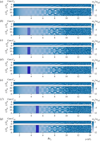
Contours of the instantaneous spanwise vorticity at  $z/\delta _{in}=8.4$ and
 $y/\delta _{in}=1.1$ for cases
 $C_{0}$,
 $C_{ll}$,
 $C_{lm}$,
 $C_{lh}$,
 $C_{nl}$,
 $C_{nm}$ and
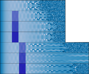
 $C_{nh}$ are displayed in figure 10. The rope-like structure is clearly seen in the
 $x$–
 $y$ plane (sideview) of case
 $C_0$ in figure 10(a). The rope-like structure is lifted up from the wall, then the tip of these structures break up into small-scale structures at
 $Re_x\approx 9 \times 10^{5}$, where the amplitude of modes (1,1) (1,3) and (1,5) begin to drop (see figure 9). Downstream
 $Re_x\approx 9 \times 10^{5}$, the small-scale structures contaminate the entire spanwise width of the computational domain and transition to turbulence finally (see figure 10a). It is observed from figures 10(b), 10(c) and 10(d) that the appearance of small-scale structures for the case with narrow cooling strips in the linear region is more downstream than that of case
 $C_0$, which means the occurrence of oblique breakdown for cases
 $C_{ll}$,
 $C_{lm}$ and
 $C_{lh}$ is shifted downstream compared with case
 $C_0$. However, the shifted distance does not increase as the wall temperature decreases. When the temperature is set to
 $T=0.25T_w$, oblique breakdown occurs more upstream than for case
 $C_{lm}$ (
 $T=0.50T_w$) and almost at the same streamwise position as case
 $C_{ll}$ (
 $T=0.75T_w$). The reason for the transition onset differences will be given in § 3.3.
Instantaneous contours of spanwise vorticity  $\omega _z$ at
 $z/\delta _{in}=8.4$ and
 $y/\delta _{in}=1.1$ for (a) Case
 $C_0$, (b)
 $C_{ll}$, (c)
 $C_{lm}$, (d)
 $C_{lh}$, (e)
 $C_{nl}$, ( f)
 $C_{nm}$ and (g)
 $C_{nh}$, respectively. The local cooling strips with temperatures
 $0.75T_w$,
 $0.50T_w$ and
 $0.25T_w$ are denoted by blue strips; the deeper the colour is, the lower the temperature of the cooling strips. The
 $\omega _{ref}$ is defined as
 $u_{\infty }/L_{ref}$.

When the cooling strips are set at the early nonlinear region (see figures 10e, 10f and 10g), the occurrence of oblique breakdown shifts downstream due to the cooling strip. It is observed that the cooling position has influence on the transition onset. For example, the position of flow breakup for case  $C_{nm}$ (figure 10f) is slightly downstream than case
 $C_{lm}$ (figure 10c). We speculate that nonlinear mechanisms are responsible for this difference. Thus, we increase the width of the cooling strip to
 $5.5~\mathrm {mm}$ to magnify the transition onset differences and find the mechanism responsible for the differences.
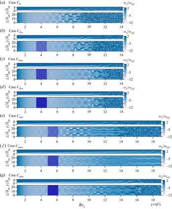
Contours of the instantaneous spanwise vorticity at  $z/\delta _{in}=8.4$ and
 $y/\delta _{in}=1.1$ for cases
 $C_{0}$,
 $C_{llw}$,
 $C_{lmw}$,
 $C_{lhw}$,
 $C_{nlw}$,
 $C_{nmw}$ and
 $C_{nhw}$ are displayed in figure 11. To capture the oblique breakdown, a longer domain is used for cases
 $C_{nlw}$,
 $C_{nmw}$ and
 $C_{nhw}$. With the increasing of cooling width, oblique breakdown occurs more downstream than narrow cooling strips (see figures 11b, 11c and 11d). When wider cooling strips are set in the early nonlinear region, the influence of cooling position on transition onset is amplified (see figures 11e, 11f and 11g). First, the transition onset occurs far downstream than the cooling strip in the linear region with the same width and temperature. Second, the temperature of the cooling strips has a great effect on the transition onset. When the temperature of the cooling strip is set to
 $0.50T_w$, no turbulent region is observed in the computational domain (see figure 11f). However, the transition occurs in both cases
 $C_{nlw}$ (figure 11e) and
 $C_{nhw}$ (figure 11g). The above phenomena will be illustrated in §§ 3.3, 3.4 and 3.5.
Instantaneous contours of spanwise vorticity  $\omega _z$ at
 $z/\delta _{in}=8.4$ and
 $y/\delta _{in}=1.1$ for (a) Case
 $C_0$, (b)
 $C_{llw}$, (c)
 $C_{lmw}$, (d)
 $C_{lhw}$, (e)
 $C_{nlw}$, ( f)
 $C_{nmw}$ and (g)
 $C_{nhw}$, respectively. The local cooling strips with temperatures
 $0.75T_w$,
 $0.50T_w$ and
 $0.25T_w$ are denoted by blue strips, the colour is deeper, and the temperature of the cooling strips is lower. The
 $\omega _{ref}$ is defined as
 $u_{\infty }/L_{ref}$.

Next, we will provide the quantified results of transition onset. As the results obtained by different definitions of transition onset are inconsistent (Stetson & Kimmel Reference Stetson and Kimmel1992), several transition onset criteria (Franko & Lele Reference Franko and Lele2013) are used, namely, the streamwise evolution of the skin friction coefficient ( $C_f$), boundary layer (
 $\delta$) and momentum thickness (
 $\theta$) (see table 4).
Streamwise position of the transition onset and maximum value of the skin-friction coefficient.

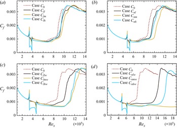
The skin friction coefficient  $C_f$ is the most widely used criterion to quantify the onset of transition. The skin friction coefficient is averaged in span and time, then the location of minimal value of the averaged
 $C_f$ is selected as the transition onset. The evolution of
 $C_f$ for cooling strips in the linear region is shown in figures 12(a) and 12(c). The overshoot of
 $C_f$ upstream of the domain is caused by the cooling strips. Downstream of the cooling strip,
 $C_f$ recovers to the value of laminar flow. The onsets of transition obtained by
 $C_f$ remain consistent with the results in figures 10 and 11. The delay effect is enhanced monotonically as the cooling width increases. However, the transition delay effect of temperature does not increase with temperature decreasing. It should be noted that the onset of flow breakup for case
 $C_{lm}$ is slightly upstream compared with case
 $C_{nm}$ (see figure 10c, f), whereas in table 4, the transition onset based on the minimum value of
 $C_f$ for case
 $C_{nm}$ is slightly downstream compared with case
 $C_{lm}$.
Evolution of the skin coefficient in the streamwise direction: (a) cases with a narrow cooling strip in the linear region; (b) cases with a narrow cooling strip in the early nonlinear region; (c) cases with a wider cooling strip in the linear region; and (d) cases with a wider cooling strip in the early nonlinear region.

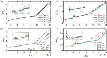
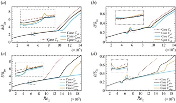
The streamwise evolutions of the boundary layer and momentum thickness for all the cases are shown in figures 13 and 15. The boundary layer thickness is defined at wall-normal position where the streamwise velocity reaches  $99\,\%$ of the free stream velocity
 $u_\infty$. The momentum thickness is defined as follows:
 \begin{equation} \theta=\int_{0}^{\infty}\frac{\rho u}{\rho_\infty u_\infty}\left(1-\frac{u}{u_\infty}\right) \mathrm{d} y. \end{equation}
Evolution of the boundary layer and momentum thickness in the streamwise direction with cooling strip at the linear region. (a,c) Boundary layer and momentum thickness of cases  $C_0$,
 $C_{ll}$,
 $C_{lm}$ and
 $C_{lh}$, respectively; (c,d) boundary layer and momentum thickness of cases
 $C_0$,
 $C_{llw}$,
 $C_{lmw}$ and
 $C_{lhw}$, respectively.

The transition onset based on the boundary layer thickness is defined as the location where the thickness departs  $5\,\%$ from the laminar value (Franko & Lele Reference Franko and Lele2013). However, this definition is not suitable for momentum thickness owing to the oscillation of momentum thickness for cooled cases. In figures 13 and 15, the growth rate of the boundary layer thickness slows before it rises rapidly, which can also be seen in Franko & Lele (Reference Franko and Lele2014). Thus, we define the transition onset of momentum and boundary layer thickness where the growth rate of thickness is least before the boundary grows rapidly (see table 4). It can be observed that the transition onset using boundary layer thickness as a criterion is more downstream than using
 $C_f$. However, it makes no difference in the relative transition onsets between different cases with different criteria.
In both figures 13 and 15, the cooling strips will make the boundary layer thinner within the cooling region. However, the thickness of the boundary layer does not decrease as the cooling temperature decreases. In figure 13(a), the boundary layer thickness of case  $C_{lh}$ is thicker than that of case
 $C_{lm}$ within the cooling region. A similar situation for cases
 $C_{lhw}$ and
 $C_{lmw}$ can also be seen in figure 15(a). Downstream of the cooling strip, the boundary layer thickness of case
 $C_{lh}$ is thicker than that of case
 $C_{0}$ without cooling.
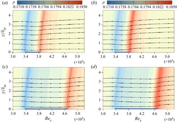
The pressure contour and streamlines around the cooling strips for cases  $C_{lm}$ and
 $C_{lh}$ are shown in figures 14(a) and 14(b), respectively. It is observed that the streamlines are lowered down at the beginning of cooling strips (
 $\textit {Re}_x=3.37\times 10^{5}$) due to the expansion waves, while the streamlines are lifted up due to the compression waves at the end of cooling strip (
 $\textit {Re}_x=3.85\times 10^{5}$), which means the boundary layer becomes increasingly thicker (Soudakov et al. Reference Soudakov, Egorov and Fedorov2009). With the lowering of the cooling temperature, the pressure becomes higher at the end of the strip. Due to the higher pressure for case
 $C_{lh}$, the boundary layer of case
 $C_{lh}$ is thicker than case
 $C_{lm}$ within the cooling strip and lifted higher than case
 $C_{0}$ downstream of the cooling strip, which is consistent with the results in figure 13(a). When the cooling strip is wider, the boundary layer thickness for case
 $C_{lhw}$ is slightly lower than that for case
 $C_{lmw}$ (figure 13c). Although the compression wave for case
 $C_{lhw}$ is stronger than that for case
 $C_{lh}$ (see figure 14b,d), the boundary layer of case
 $C_{lhw}$ is thinner than that of case
 $C_{0}$ downstream of the cooling strip (figure 13c), whereas case
 $C_{lh}$ is thicker than that of case
 $C_{0}$ downstream of the cooling strip (figure 13a); because the thickness of the boundary layer becomes lower for case
 $C_{lhw}$ than
 $C_{lh}$ before reaching the end of the cooling strip. For cooling strips in the early nonlinear region, the variation trend of boundary layer thickness around the cooling strips is similar to that of the cooling strips in the linear region (see figures 15a and 15c). In addition, the evolution of momentum thickness remains consistent with the boundary layer thickness, which becomes thinner and then thicker.
Instantaneous contours of pressure and streamlines around the cooling strip area for (a) case  $C_{lm}$, (b) case
 $C_{lh}$, (c) case
 $C_{lmw}$ and (d) case
 $C_{lhw}$. The cooling strips are denoted as thin blue rectangle strips at the bottom of the contours.

Evolution of the boundary layer and momentum thickness in the streamwise direction with cooling strip at the early nonlinear region. (a,c) Boundary layer and momentum thickness of cases  $C_0$,
 $C_{nl}$,
 $C_{nm}$ and
 $C_{nh}$, respectively; (c,d) boundary layer thickness of cases
 $C_0$,
 $C_{nlw}$,
 $C_{nmw}$ and
 $C_{nhw}$, respectively.

Although the transition onset has some differences using different criteria, the relative transition positions are consistent. From the above results, the effect of the cooling strip on the transition onset is concluded as follows. First, the onset of the transition will be delayed with cooling strips. However, the onset of the transition does not vary monotonically with temperature. The delay effect will be better when the temperature is set to  $0.50T_w$, which is inconsistent with the LST results (see § 3.1). Second, the position of the cooling strip plays an important role in the transition onset. When the cooling strips are employed in the early nonlinear region with a wider width, the transition occurs far downstream. Why does the transition onset not vary monotonously with temperature? What is the mechanism responsible for the great influence of the cooling position on the transition onset? These two questions will be answered in the following sections.
3.3. Local cooling strip at linear region
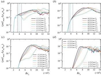
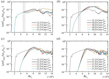
To analyse the delay mechanism of the cooling strip on oblique breakdown, Fourier transformation in both time and spanwise directions is conducted for each flow field (see § 2.5). Figure 16 shows that the transition delay is due to the damping effect of cooling strips on the fundamental oblique waves (1,1) (figure 16a). The fundamental oblique waves (1,1) serve as an ‘actuator’ that introduces disturbance into modes (0,2) (Laible & Fasel Reference Laible and Fasel2016). Thus, the damping of mode (1,1) will lead to the slowing growth rate of the steady mode (0,2) (figure 16b). Then the strength of the wave–vortex triad composed of modes (1,1) and (0,2) are weakened, results in the growth rate of higher modes (1,3) and (1,5) generated by the mutual interaction between wave–vortex triads slowing down (see figures 16c and 16d). Eventually, the transition is delayed with local cooling owing to the slowing growth rate of mode (1,1). Therefore, we will focus on the damping effect of the cooling strip on the evolution of the ‘actuator’ mode (1,1) in the streamwise direction in the following paragraphs.
Various mode developments in the streamwise direction for cases with cooling strips in the linear region of oblique breakdown: (a) fundamental oblique mode (1,1); (b) steady vortex mode (0,2); (c,d) for higher harmonic modes (1,3) and (1,5), respectively. The cooling strips are indicated by the vertical dashed lines, and the green and blue vertical dashed lines represent the ends of the narrow and wider cooling strips, respectively.

To better investigate the evolution of mode (1,1) in the streamwise, the growth rate ( $-\alpha _i$) of mode (1,1) is defined as follows:
 \begin{equation} {-}\alpha_i=\frac{\mathrm{d}}{\mathrm{d} x}\ln(A(x)). \end{equation}
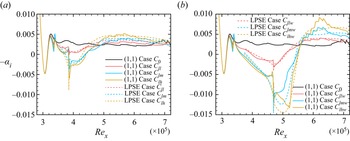
The growth rate of mode (1,1) of the case with cooling strip at the linear region is shown in figure 17. It is observed that the evolution of mode (1,1) experiences three stages.
Evolution of the growth rate of mode (1,1) in the streamwise direction: (a) case  $C_0$,
 $C_{ll}$,
 $C_{lm}$ and
 $C_{lh}$; (b) case
 $C_0$,
 $C_{llw}$,
 $C_{lmw}$ and
 $C_{lhw}$. The cooling strips are indicated by the vertical dashed lines. The dashed lines represent the results solved by the linear parabolic stability equation (LPSE).

The first stage is within the region of cooling strip. For the narrow cooling strip case, this stage extends from  $\textit {Re}_x\approx 3.37\times 10^{5}$ to
 $\textit {Re}_x\approx 3.85\times 10^{5}$, which is from
 $\textit {Re}_x\approx 3.37\times 10^{5}$ to
 $\textit {Re}_x\approx 4.81\times 10^{5}$ for case with wide cooling strip. At this stage, the local cooling strip results in the decreasing of the growth rate of mode (1,1) compared with that of case
 $C_0$. The growth rate of mode (1,1) becomes smaller as the cooling temperature is lower (see figures 17a and 17b). In addition, compared with the case with narrow cooling strips, the wider cooling strip will lead to a lower growth rate of mode (1,1) at the end of this stage. For instance, the growth rate of mode (1,1) of case
 $C_{lh}$ is approximately 0 at
 $\textit {Re}_x\approx 3.85\times 10^{5}$, which is approximately −0.011 for case
 $C_{lhw}$ at
 $\textit {Re}_x\approx 4.81\times 10^{5}$.
The second stage begins from the end of cooling strip, then ends at the station where the growth rate of mode (1,1) for the cooled case is equal to that of  $C_0$. For example, the end of the second stage for case
 $C_{lh}$ is at
 $\textit {Re}_x\approx 4.7\times 10^{5}$ where the growth rate of mode (1,1) of case
 $C_{lh}$ is equal to that of case
 $C_0$ (see figure 17a). At the beginning of this stage, the growth rate of mode (1,1) for cooled case is smaller than that within the cooing strip. Then the growth rate of mode (1,1) becomes greater with the evolution in the streamwise direction until it reaches the same growth rate of case
 $C_0$ at the end of this stage.
The third stage begins at where the growth rate of mode (1,1) of cooled case is greater than that of case  $C_0$. For instance, case
 $C_{lh}$ begins from
 $\textit {Re}_x\approx 4.7\times 10^{5}$. At this stage, the growth rate of mode (1,1) of the cooled case is greater than case
 $C_0$. As the cooling temperature becomes lower, the growth rate of mode (1,1) is greater than that of case
 $C_0$, which is the reason that the transition onset of case
 $C_{lh}$ is more upstream than case
 $C_{lm}$. In addition, the case with the wider cooling strip will result in greater maximal growth rate of mode (1,1) than the case with narrow cooling strip with same temperature at this region. For example, the maximal growth rate of mode (1,1) for case
 $C_{lh}$ is approximately 0.005 at
 $\textit {Re}_x\approx 5.7\times 10^{5}$, which is approximately 0.009 for case
 $C_{lhw}$ at
 $\textit {Re}_x\approx 6.2\times 10^{5}$; (see figures 17a and 17b).
It should be noted that when the narrow cooling strip is embedded at an adiabatic wall, the transition onset is almost proportional to the cooling temperature (Zhou et al. Reference Zhou, Lu, Liu and Yan2021). However, the transition onset does not change monotonically with cooling temperature in the current study, for the reason that the growth rate of mode (1,1) of the cooled case will become greater with the cooling temperature becoming lower at the third stage (see figure 17).
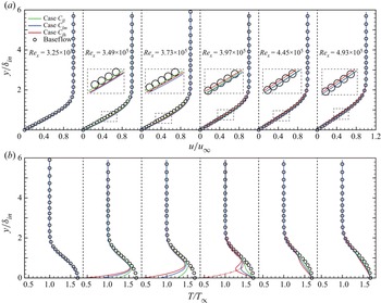
To illustrate the three stages of the evolution of mode (1,1) in figure 17, especially, the growth rate of mode (1,1) of cooled case is greater than that of case  $C_0$ at the third stage, the time-averaged profiles of streamwise velocity and temperature in the wall-normal direction around the cooling strips for cases
 $C_{ll}$,
 $C_{lm}$ and
 $C_{lh}$ are shown in figure 18. It is observed that the cooling strips have less influence on both the streamwise velocity and temperature profiles upstream of the cooling strip (
 $\textit {Re}_x\approx 3.25\times 10^{5}$) (see figure 18). In addition, the cooling strips have less influence on the streamwise velocity profile. Even within the cooling area, the profile of the streamwise velocity is slightly thinner than that of the baseflow. However, the cooling strips have a great impact on the profile of the temperature, which is most likely to lead to the growth rate of the mode (1,1) variation in the streamwise direction.
Time-averaged streamwise velocity and temperature profiles of cases  $C_{ll}$,
 $C_{lm}$ and
 $C_{lh}$. Here
 $\textit {Re}_x=3.25\times 10^{5}$ is slightly upstream of the cooling strip;
 $\textit {Re}_x=3.49\times 10^{5}$ and
 $\textit {Re}_x=3.73\times 10^{5}$ are within the cooling strip;
 $\textit {Re}_x=3.97\times 10^{5}$,
 $\textit {Re}_x=4.45\times 10^{5}$ and
 $\textit {Re}_x=4.93\times 10^{5}$ are downstream of the cooling strip. Symbol circles indicate the variable distribution from the baseflow of case
 $C_0$ without disturbance. (a) Streamwise velocity distribution; (b) temperature distribution. The red dashed line in the fourth subpanel of figure (b) represents the temperature profiles of case
 $C_{lh}$ at
 $\textit {Re}_x=3.73\times 10^{5}$

The evolution of temperature profiles in the streamwise direction are shown in figure 18(b). First, the temperature profile changes over the cooling area due to the cooling strip ( $\textit {Re}_x=3.49\times 10^{5}$ and
 $\textit {Re}_x=3.73\times 10^{5}$). As cooling temperatures are lower, the temperature profile deviates more from the baseflow, which is the reason for the growth rate decreasing of mode (1,1) for case
 $C_{ll}$,
 $C_{lm}$ and
 $C_{lh}$ at the first stage of the evolution of mode (1,1) (see figure 17a).
Second, slightly downstream of the end of the cooling strips ( $\textit {Re}_x=3.97\times 10^{5}$), the profile of the temperature close to the wall is recovered to the temperature of the wall. However, the profile of temperature far from the wall (approximately
 $y/\delta _{in} > 0.5$) remains consistent with the profile of temperature within the cooling strip (
 $\textit {Re}_x=3.73\times 10^{5}$) and even deforms more than that within the cooling strip; see the fourth segment of figure 18(b), which is consistent with the results of Fedorov et al. (Reference Fedorov, Soudakov, Egorov, Sidorenko, Gromyko, Bountin, Polivanov and Maslov2015). This is the reason that the growth rate of mode (1,1) of case
 $C_{lh}$ at
 $\textit {Re}_x=3.97\times 10^{5}$ is smaller than that at
 $\textit {Re}_x=3.73\times 10^{5}$ (see figure 17a). With the evolution of the temperature profile in the streamwise direction, the temperature profiles of case
 $C_{ll}$,
 $C_{lm}$ and
 $C_{lh}$ are gradually closer to the temperature profile of the baseflow (from
 $\textit {Re}_x=3.97\times 10^{5}$ to
 $\textit {Re}_x=4.45\times 10^{5}$). This is the reason for the growth rate of mode (1,1) of the cooled case being gradually closer to that of case
 $C_0$ at the end of the second stage in figure 17(a). Additionally, it is observed from figure 17 that the evolution of the growth rate of mode (1,1) solved by the LPSE agree with that of DNS approximately for various cases, which is the proof of the claims made above.
Although the temperature profiles of case  $C_{ll}$,
 $C_{lm}$ and
 $C_{lh}$ are close to that of the baseflow at
 $\textit {Re}_x=4.93\times 10^{5}$, the temperature gradient near the wall is not recovered to zero (see figure 19a). Furthermore, the temperature gradient near the wall increases with the decreasing of cooling temperature. The temperature gradient near the wall means thermomechanical non-equilibrium, which will lead to the transition onset occurring more upstream than the thermomechanical equilibrium wall in a Mach 2.2 boundary layer (Sharma, Shadloo & Hadjadj Reference Sharma, Shadloo and Hadjadj2019a). This is the reason that the growth rate of mode (1,1) for case
 $C_{lh}$ is greater than that of cases
 $C_{lm}$ and
 $C_{ll}$ at the third stage (see figure 17a).
(a) Wall-normal temperature gradient of case  $C_{ll}$,
 $C_{lm}$,
 $C_{lh}$ and laminar baseflow of case
 $C_0$ at
 $\textit {Re}_x=4.93\times 10^{5}$. (b) Generalized inflection point curve for case
 $C_{lh}$ at
 $Re_x=3.25\times 10^{5}$,
 $Re_x=3.73\times 10^{5}$,
 $Re_x=3.97\times 10^{5}$ and
 $Re_x=4.93\times 10^{5}$; the horizontal dashed lines indicate the location at which
 $u=1-1/Ma_{\infty }$.

To further confirm the stability state of mode (1,1) during the three stages, the generalized inflection point (GIP) is defined as follows (Mack Reference Mack1984; Sharma et al. Reference Sharma, Shadloo, Hadjadj and Kloker2019b):
 \begin{equation} {\rm GIP}(y): \frac{\mathrm{d}}{\mathrm{d} y}\left(\rho \frac{\mathrm{d}u}{\mathrm{d} y}\right)_{y=y_s}=0. \end{equation}
If  $y_s>y_0$ (
 $y_0$ is the point at which
 $u=1-1/Ma_{\infty }$), it signifies the existence of inviscid instability in the meanflow (Lees & Lin Reference Lees and Lin1946). The GIPs for cases
 $C_{lh}$ is denoted in figure 19(b). No GIP exists within the cooling region (
 $Re_x=3.73\times 10^{5}$) for case
 $C_{lh}$. Slightly downstream of the cooling strip (
 $Re_x=3.97\times 10^{5}$), GIP exists for both cases; however, the value of
 $y_s$ is less than
 $y_0$, which is consistent with the growth rate of mode (1,1) slowing around
 $Re_x=3.97\times 10^{5}$. At the upstream (
 $Re_x=3.25\times 10^{5}$) and far downstream (
 $Re_x=4.93\times 10^{5}$) of the cooling strip, GIPs are generated and satisfy the condition
 $y_s>y_0$, and mode (1,1) of case
 $C_{lh}$ is amplified at the two stations.
3.4. Narrow local cooling strip in the early nonlinear region
The evolution of various modes for cases  $C_{nl}$,
 $C_{nm}$,
 $C_{nh}$ and
 $C_0$ are demonstrated in figure 20. The delay mechanism of the cooling strip on oblique breakdown in the early nonlinear region with narrow cooling strips is similar to the cooling strip in the linear region. The cooling strip changes the temperature profile of the baseflow, leading to the damping of mode (1,1) (figure 20a). Then, the growth rate of mode (0,2) slows down (figure 20b). Subsequently, the wave–vortex triads composed of modes (1,1) and (0,2) are weakened, leading to the growth rate of modes (1,3) and (1,5) slowing down (figure 20c,d). Eventually, the oblique breakdown is delayed.
Various mode developments in the streamwise direction for cases  $C_0$,
 $C_{nl}$,
 $C_{nm}$ and
 $C_{nh}$: (a) initial oblique mode (1,1); (b) steady vortex mode (0,2); (c,d) for higher harmonic modes (1,3) and (1,5), respectively. The cooling strips are indicated by the vertical dashed line.

It is should be noted that the growth rate of mode (1,1) becomes faster with the decreasing of temperature downstream of the cooling strip, which is similar to the third stage of the evolution of mode (1,1) for the case with a cooling strip at linear region. For instance, the amplitude of mode (1,1) of case  $C_{nh}$ exceeds that of case
 $C_{nm}$ at
 $\textit {Re}_x\approx 7.1\times 10^{5}$, which indicates that the growth rate of mode (1,1) of case
 $C_{nh}$ is faster than that of case
 $C_{nm}$ downstream
 $\textit {Re}_x\approx 6.4\times 10^{5}$ (see figure 20a). Thus, the transition onset of case
 $C_{nh}$ is more upstream than that of case
 $C_{nm}$.
3.5. Wide local cooling strip in the early nonlinear region
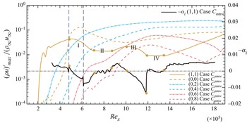
It efficiently delays the occurrence of transition when cooling strips are utilized in the early nonlinear region of oblique breakdown with wide cooling strips. It is observed from figures 21, 22 and 24 that the growth rate of fundamental mode (1,1) slows in several regions (labelled with Roman numbers), which is the reason that the transition of case with a wide cooling strip at the early nonlinear region occurs far downstream. It should be noted that the meanflow distortion (MFD) (0,0) and steady modes such as (0,2), (0,4), (0,6) and (0,8) dominate the flow where the growth rate of fundamental mode (1,1) slows down. What is more, the stabilization effect of both steady modes and meanflow distortion generated by the steady modes on the fundamental mode (1,1) has been reported in Paredes et al. (Reference Paredes, Choudhari and Li2017), Sharma et al. (Reference Sharma, Shadloo, Hadjadj and Kloker2019b) and Kneer et al. (Reference Kneer, Guo and Kloker2022). Thus, the role of steady modes and the MFD generated by the steady modes will be discussed in the following sections.
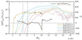
Various mode developments in the streamwise direction for case  $C_{nlw}$. The cooling strips are indicated by the vertical dashed line. The horizontal dashed–dot line represents the growth rate is equal to 0. Region I extends from
 $\textit {Re}_x\approx 4.8\times 10^{5}$ to
 $\textit {Re}_x\approx 6.6\times 10^{5}$; region II extends from
 $\textit {Re}_x\approx 6.6\times 10^{5}$ to
 $\textit {Re}_x\approx 9.4\times 10^{5}$; and region III extends from
 $\textit {Re}_x\approx 9.4\times 10^{5}$ to
 $\textit {Re}_x\approx 10.1\times 10^{5}$.

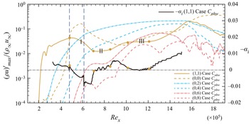
Various mode developments in the streamwise direction for case  $C_{nhw}$. The cooling strips are indicated by the vertical dashed line. The horizontal dashed–dot line represents the growth rate is equal to 0. Region I extends from
 $\textit {Re}_x\approx 4.8\times 10^{5}$ to
 $\textit {Re}_x\approx 7.0\times 10^{5}$; region II extends from
 $\textit {Re}_x\approx 7.0\times 10^{5}$ to
 $\textit {Re}_x\approx 8.6\times 10^{5}$; and region III extends from
 $\textit {Re}_x\approx 10.2\times 10^{5}$ to
 $\textit {Re}_x\approx 12.2\times 10^{5}$.

3.5.1. Role of higher spanwise wavenumber steady modes
The evolution of mode (1,1) and the steady modes of case  $C_{nlw}$ is shown in figure 21. The Roman numbers I, II and III represent three different regions where the growth rate of mode (1,1) are at a low level (close to or lower than 0) by different mechanisms. At region I, the growth rate of mode (1,1) becomes smaller with the evolution in the streamwise direction due to the stability of the boundary layer being changed by the cooling strip. At region II, the growth rate of mode (1,1) is less than 0.001, which reaches to the smallest value of approximately 0.0004 at
 $\textit {Re}_x\approx 8.2\times 10^{5}$. At region III, the growth rate of mode (1,1) keeps decreasing and reaches a value of approximately
 $-0.013$ at
 $\textit {Re}_x\approx 10.1\times 10^{5}$. When downstream region III, the amplitude of mode (1,1) grows to trigger the breakdown of the boundary layer. We spectate that the slowing growth rates of mode (1,1) of case
 $C_{nlw}$ at region II and III are similar to the phenomenon in Zhou et al. (Reference Zhou, Lu, Liu and Yan2021) that the higher spanwise wavenumber steady modes are responsible for the slowing growth rate of mode (1,1).
As shown in figure 21, when the amplitude of mode (0,4) is higher than mode (1,1) at  $\textit {Re}_x\approx 7.0\times 10^{5}$, then the growth rate of mode (1,1) is at a low level (approximately 0.0005) from
 $\textit {Re}_x\approx 7.6\times 10^{5}$ to
 $\textit {Re}_x\approx 9.4\times 10^{5}$. Similarly, when the amplitude of mode (0,8) is higher than mode (1,1) at
 $\textit {Re}_x\approx 9.6\times 10^{5}$, the growth rate of mode (1,1) is small within region III. Moreover, the growth rate of mode (1,1) at region III is smaller than that at region III, because the suppression effect of (0,8) on the mode (1,1) will be reinforced compared with that of mode (0,4) (Paredes et al. Reference Paredes, Choudhari and Li2017), which further proves the suppression effect of the higher span wavenumber steady modes on the fundamental oblique mode (1,1). We call this phenomenon the SSE in the present study, since the higher span wavenumber steady modes are generated by the mutual and self-interaction of mode (1,1) and harmonic modes. The SSE works two times for case
 $C_{nlw}$; the first time results in the slowing growth rate of mode (1,1) at region II, the second time leads to the growth rate of mode (1,1) smaller than 0 at region III (see figure 21). It is worth mentioning that the SSE works two times in Zhou et al. (Reference Zhou, Lu, Liu and Yan2021), but only one time is discovered. The combination the stabilization effect of the cooling strip and the SSE make the transition of case
 $C_{nlw}$ occur more downstream than case
 $C_{llw}$. It should be noted that the amplitude of mode (0,8) can exceed mode (0,6) to suppress the increasing of mode (1,1) (see figure 21).
Similar to case  $C_{nlw}$, the growth rate of mode (1,1) of case
 $C_{nhw}$ is at a low level in three different regions represented by Roman numbers I,II and III, respectively (see figure 22). At Region I, the growth rate of mode (1,1) decreases owing to the stabilization effect of cooling strip on mode (1,1), which reaches a value approximately
 $-0.0084$ at
 $\textit {Re}_x\approx 6.8\times 10^{5}$. At region II, the SSE is responsible for the slowing growth rate of mode (1,1) which is around 0. Specifically, the mode (0,4) results in slowing the growth rate of (1,1) at region II. Similarly, the SSE leads to the growth rate of mode (1,1) being close to 0 at region III; specifically, the stabilization of mode (0,6) on mode (1,1) works at this time.
For comparison, the streamwise evolution of modes (1,1), (0,4) and (0,6) for cases  $C_{llw}$ and
 $C_{lhw}$ are shown in figure 23(a). The cooling strips in cases
 $C_{llw}$ and
 $C_{lhw}$ are upstream of
 $C_{nlw}$ and
 $C_{nhw}$. The amplitude of mode (1,1) with cooling strips in the linear region will be suppressed once downstream of the blowing and suction strip, which is equal to shifting the blowing and suction strip to a more downstream position. The stabilization by modes (0,4) and (0,6) will not work for cases
 $C_{llw}$ and
 $C_{lhw}$, since the amplitudes of modes (0,4) and (0,6) are hard to exceed mode (1,1). When the amplitude of various modes is at the same level, oblique breakdown occurs (see figure 23a). When cooling strips in the early nonlinear region with narrow cooling strips, the stabilization effect of higher spanwise wavenumber steady modes is not obvious (see figure 23b). The amplitude of mode (0,4) exceeds that of mode (1,1) at
 $\textit {Re}_x\approx 7.5\times 10^{5}$ for case
 $C_{nm}$, where the amplitudes of modes (1,1), (0,4) and (0,6) at
 $\textit {Re}_x\approx 7.5\times 10^{5}$ are of the same order and the oblique breakdown is about to occur. Thus, the growth rate of mode (1,1) of
 $C_{nm}$ only slows down slightly compared with case
 $C_{nl}$.
Various mode developments in the streamwise direction for (a) cases  $C_{lmw}$ and
 $C_{lhw}$; (b) cases
 $C_{nl}$ and
 $C_{nm}$.

The streamwise evolution of various modes of case  $C_{nmw}$ are denoted in figure 24. Compared with case
 $C_{nlw}$ and
 $C_{nhw}$, the SSE works three times for case
 $C_{nmw}$, which results in the slowing growth rate of mode (1,1) at regions II, III and IV, respectively. At region II, the stabilization effect of mode (0,4) on mode (1,1) works from
 $\textit {Re}_x\approx 7.1\times 10^{5}$ to
 $\textit {Re}_x\approx 9.0\times 10^{5}$ for the first time. At the second time, both the stabilization effect of mode (0,6) and (0,8) work at this time and make the growth rate of mode (1,1) decrease to
 $-0.013$ at
 $\textit {Re}_x\approx 11.8\times 10^{5}$ (region III). At region IV , the SSE works for the third time, which leads to the growth rate of mode (1,1) around 0. At region I, the stabilization effect of cooling strip on mode (1,1) results in the growth rate decreasing of mode (1,1). Eventually, oblique breakdown of case
 $C_{nmw}$ is delayed to occur more downstream than cases
 $C_{nlw}$ and
 $C_{nhw}$, and no turbulence region exists.
Various mode developments in the streamwise direction for case  $C_{nmw}$. The cooling strips are indicated by the vertical dashed line. The horizontal dashed–dot line represents the growth rate is equal to 0. Region I extends from
 $\textit {Re}_x\approx 4.8\times 10^{5}$ to
 $\textit {Re}_x\approx 7.1\times 10^{5}$; region II extends from
 $\textit {Re}_x\approx 7.1\times 10^{5}$ to
 $\textit {Re}_x\approx 9.0\times 10^{5}$; region III extends from
 $\textit {Re}_x\approx 10.1\times 10^{5}$ to
 $\textit {Re}_x\approx 12.0\times 10^{5}$; and region IV extends from
 $\textit {Re}_x\approx 12.0\times 10^{5}$ to
 $\textit {Re}_x\approx 13.6\times 10^{5}$.

3.5.2. The role of MFD
Case  $C_{nmw}$ is employed to discuss the role of the MFD in the SSE. The MFD (0,0) in figure 24 is generated by both the cooling strip and high amplitude of steady modes.
The cooling strip will lead to the MFD around the cooling strip, which will change the temperature profile. When the cooling strip is employed at the linear region, it will result in the growth rate of mode (1,1) slowing down around the cooling strip at the first stage and the growth rate of mode (1,1) of the cooled case greater than that of case  $C_0$ at the third stage (see figure 17). When the wide cooling strip is employed at the early nonlinear region, this MFD will lead to the amplitude decreasing of the mode (1,1) at region I (see figure 24). The amplitude decreasing of mode (1,1) at region I is the trigger condition for the SSE. In addition, the strength of the SSE will not be enhanced with the decreasing of cooling temperature, since this MFD will result in the growth rate of mode (1,1) of cooled cases greater than that of case
 $C_0$ downstream the cooling strip (see figure 17). Specifically, the strength of SSE of case
 $C_{nmw}$ is stronger than that of
 $C_{nhw}$ (see figures 22 and 24). Thus, the MFD generated by the cooling strip will weaken the strength of the SSE.
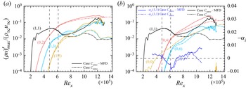
Except for the MFD generated by the cooling strip, the high amplitude of the steady modes will lead to a high amplitude of the MFD (0,0) at the downstream of the domain (see figure 25b). Following the work of Kneer et al. (Reference Kneer, Guo and Kloker2022), a nonlinear disturbance formulation (Kurz & Kloker Reference Kurz and Kloker2016) is employed to investigate the contribution of MFD generated by the steady modes on the SSE for case  $C_{nmw}$, quantitatively. There are two steps. First, a simulation using only a cooling strip is conducted, then we get a baseflow with the MFD only generated by the cooling strip, termed modified base flow (MBF). Second, a nonlinear disturbance formulation is employed to simulate the evolution of disturbances in the MBF. Specifically, the temporal derivative of the MBF generated by only a cooling strip is calculated in a preprocessing step and subtracted at each time step to keep this MBF. Thus, the MFD generated by the steady modes will be eliminated from the flow. Actually, the MFD downstream of the domain is generated by various modes, but the steady modes such as (0,2) and (0,4) will dominate the flow for case
 $C_{nmw}$. Thus, this MFD is considered to be generated by steady modes, approximately.
Evolution of (a) modes (1,1) and harmonic modes; (b) modes (1,1), (0,0) and steady modes. The solid and dash–dot lines represent the results of case  $C_{nmw}$ without and with MFD that generated by steady modes. The vertical dashed lines represent the location of cooling strip, horizontal lines represent the growth rate is 0.

The evolution of various modes for case  $C_{nmw}$ without MFD generated by the steady modes are shown in figure 25. For comparison, various modes of case
 $C_{nmw}$ are also plotted in figure 25. It is observed from figure 25(a) that the fundamental modes (1,1) and modes generated by the wave–vortex triad for case
 $C_{nmw}$ without the MFD are faster than those of case
 $C_{nmw}$. Meanwhile, the region III and IV in figure 24 do not exist in figure 25, and only part of region II (from
 $\textit {Re}_x\approx 7.0\times 10^{5}$ to
 $\textit {Re}_x\approx 8.0\times 10^{5}$) is observed in figure 25(b), where the stabilization effect of mode (0,4) on the mode (1,1) for case
 $C_{nmw}$ without the MFD works for a short distance in streamwise direction resulting in the growth rate of mode (1,1) being kept at
 $-\alpha _i\approx 0.001$. There are two reasons leading to the short region II and the vanishing of region III and IV for case
 $C_{nmw}$ without MFD. First, the growth rate of various modes such as (1,3) (0,4), (0,6) for case
 $C_{nmw}$ without MFD is faster than that with MFD, which leads to a rapid breakdown of the flow, and the stabilization of mode (0,4) only works for a short distance in the streamwise direction. Second, the mode (0,0) generated by the steady modes has a stabilization effect on the mode (1,1), which has been reported in Paredes et al. (Reference Paredes, Choudhari and Li2017), Sharma et al. (Reference Sharma, Shadloo, Hadjadj and Kloker2019b) and Kneer et al. (Reference Kneer, Guo and Kloker2022). Lacking the stabilization effect of MFD on mode (1,1), mode (1,1) grows faster than that of case
 $C_{nmw}$ leading to the amplitude of mode (0,6) not exceeding the amplitude of mode (1,1). Thus, the stabilization effect of mode (0,6) on mode (1,1) cannot work. The two reasons result in the vanishing of region III and IV, and only part of region II is reserved for case
 $C_{nmw}$ without MFD. Eventually, the oblique breakdown for case
 $C_{nmw}$ without MFD occurs at
 $\textit {Re}_x\approx 12\times 10^{5}$, which is more upstream than that of case
 $C_{nmw}$.
From the results of cases  $C_{nlw}$,
 $C_{nmw}$ and
 $C_{nhw}$, it can be concluded that there are three requirements when the cooling strips are able to trigger the SSE on mode (1,1). The first is that the spanwise wavenumbers of steady modes are at least two times greater than that of mode (1,1) (Paredes et al. Reference Paredes, Choudhari and Li2017). The second is that the amplitude of steady modes should exceed that of mode (1,1). Last, the amplitude of mode (1,1) cannot be at a high level, and nonlinear interaction between various modes is not saturated.
3.6. Effect of soften edge of local cooling strip
Case  $C_{nh}$ with a linear soften edge is employed to study the influence of cooling profile on the transition onset. As mentioned in § 2.4, the soften width is set to
 $b=1 \mathrm {mm}$ (see figure 5). The evolution of various modes and skin-friction coefficient for case
 $C_{nh}$ with flat cooling profile and soften edge are shown in figures 26(a) and 26(b), respectively. The amplitude of mode (1,1) for case
 $C_{nh}$ with soften edge will drop to a lower value than that of case
 $C_{nh}$ with flat cooling profile around
 $\textit {Re}_x\approx 6.0\times 10^{5}$. And the slope of amplitude growth of mode (1,1) for case
 $C_{nh}$ with soften edge is slightly smaller than that of case
 $C_{nh}$ with a flat cooling profile downstream
 $\textit {Re}_x\approx 6.0\times 10^{5}$, which leads to the amplitude of mode (0,2) and (1,3) being smaller than that of case
 $C_{nh}$ with a flat cooling profile at the same streamwise station (see figure 26a). Eventually, the transition onset of case
 $C_{nh}$ with soften edge occurs at more downstream than that with flat cooling profile (see figure 26b).
Evolution of (a) various modes and (b) skin-friction coefficient for case  $C_{nh}$ with flat cooling profile and soften edge.

4. Conclusions
In this paper, the control effect of cooling strips with temperature jumps at two different regions with various widths and temperatures on oblique breakdown in a supersonic boundary layer is investigated using DNS and LST. From the results of LST, the cooling wall can suppress the amplification of the disturbance with fundamental frequency and spanwise wavelength, and the damping rate is enhanced with decreasing wall temperature. However, the results obtained by DNS show that the transition onset does not vary monotonically with a temperature decrease. Moreover, both the cooling location and temperature play an important role in controlling the oblique breakdown.
When the cooling strips are utilized at the linear region of the oblique breakdown, the oblique breakdown is delayed due to the stabilization effect of cooling strips on mode (1,1). The evolution of mode (1,1) of cooled cases in the streamwise direction can be divided into three stages. The first stage is within the region of cooling strips, where the stabilization effect of the cooling strips on mode (1,1) will be enhanced with a decrease in the cooling temperature. In the second stage, the cooling strip will change the temperature profile of the baseflow downstream of the cooling strips, which makes the growth rate of mode (1,1) at the beginning of the second stage lower than that in the first stage and then gradually closer to that of the baseline case  $C_0$ at end of this stage. In the third stage, the thermomechanical non-equilibrium effect will lead to the growth rate of mode (1,1) of cooled case being greater than that of baseline case. The temperature is lower, the growth rate of mode (1,1) is greater than that of the baseline case. Eventually, the transition onset of the cooling strip at a lower temperature might occur more upstream than at a higher temperature. Additionally, the evolution of mode (1,1) of the case with a narrow cooling strip in the early nonlinear region is similar to that of the case with a cooling strip in the linear region.
When wider cooling strips are set in the early nonlinear region of oblique breakdown, except for the stabilization effect of cooling strip on mode (1,1), a SSE will be triggered, the combination of the two mechanisms makes the oblique breakdown occur far downstream of the domain. The SSE is that the growth rate of mode (1,1) is suppressed by the higher spanwise wavenumber steady modes which are generated by the mutual and self-interaction between mode (1,1) and harmonic modes during the nonlinear stage of the oblique breakdown. Further research has shown that the MFD (0,0) generated by the steady modes play an important role in SSE. This MFD has a stabilization effect on mode (1,1), which is consistent with the results of Paredes et al. (Reference Paredes, Choudhari and Li2017), Sharma et al. (Reference Sharma, Shadloo, Hadjadj and Kloker2019b) and Kneer et al. (Reference Kneer, Guo and Kloker2022). It is observed that the SSE works three times, and results in the growth rate of fundamental mode (1,1) slowing down at three different regions for case  $C_{nmw}$, respectively. Meanwhile, the stabilization of modes (0,4), (0,6) and (0,8) on mode (1,1) are observed, only the stabilization effect of mode (0,4) on mode (1,1) is observed in Zhou et al. (Reference Zhou, Lu, Liu and Yan2021). When the MFD generated by the steady modes is subtracted from the baseflow, the growth rate of various modes will become fast, and the SSE only works one time. Eventually, the occurrence of oblique breakdown for the case without MFD is more upstream than that of the case with MFD. Similar to the linear region, the delay effect does not vary monotonically with cooling temperature, as the strength of SSE will be weakened with the decreasing of cooling temperature.
There are three requirements needed to trigger the SSE. The first is that the spanwise wavenumbers of steady modes are at least two times greater than those of mode (1,1) (Paredes et al. Reference Paredes, Choudhari and Li2017). The second is that the amplitude of steady modes should exceed that of mode (1,1). Last, the amplitude of mode (1,1) cannot be at a high level, and nonlinear interaction between various modes is not saturated. Thus, the cooling strip in the linear region or in the early nonlinear region with a narrow cooling width cannot trigger the SSE.
At last, the cooling profile with soften edge will enhance the stabilization of cooling strip on the fundamental mode (1,1) compared with the flat cooling profile with temperature jump at the cooling edge, which makes the oblique breakdown occur at more downstream than the case with a flat cooling profile.
Acknowledgements
The authors would like to acknowledge Professor X. Li (Institute of Mechanics, Chinese Academy of Sciences) for the DNS code OpenCFD. The fruitful discussion with Dr M. Kloker (IAG, Universität Stuttgart) on ‘Nonlinear disturbance formulation’ are gratefully acknowledged.
Funding
This study is supported by grants from the National Numerical Wind Tunnel Project of China (no. NNW2019ZT1-A03) and the National Natural Science Foundation of China (grant no. 11721202).
Declaration of interests
The authors report no conflict of interest.
Appendix A. Grid sensitivity studies
Grid sensitivity studies are conducted to validate the grid resolution. The details of the cases used for the grid sensitivity study are shown in table 5. Exceptional agreement for the streamwise evolution of various modes between cases  $C_0$ and
 $C_{{0,coarse}}$ is observed in figure 27(a).
Details of cases for the grid sensitivity study.

Grid sensitivity study: (a) streamwise evolution of various modes for cases  $C_{nh}$ and
 $C_{nh,coarse}$; (b) distribution of the Stanton number for cases
 $C_0$ and
 $C_{0,coarse}$; (c) van Driest velocity profiles at
 $\textit {Re}_x=14\times 10^{5}$; and (d) skin friction distribution of cases
 $C_0$ and
 $C_{0,coarse}$.

Additionally,  $C_f$ corresponds well to the turbulent correlation formula at the end of domain where the boundary layer is breaking to fully developed turbulence, and
 $St$ is slightly lower than the estimated value (see figures 27d and 27b, respectively). The skin friction coefficient
 $C_f$ and Stanton number
 $St$ are defined as
 \begin{equation} C_f=\frac{\tau_w}{\frac{1}{2}\rho_\infty u^{2}_\infty}, \quad S_t=\frac{q_w}{\rho_\infty u_\infty C_p(T_{aw}-T_w)}, \end{equation}
respectively. The  $T_{aw}$ can be calculated by (2.5) estimated with a recovery factor of
 $r=Pr^{1/3}$. The turbulent correlations formula is given by White (Reference White2006) and Bradshaw (Reference Bradshaw1977). Last, the van Driest transform (Van Driest Reference Van Driest1951) is used to compute the Reynolds- and spanwise-averaged van Driest velocity
 $U^{+}_{VD}$, where
 \begin{equation} y^{+}=\frac{\rho_w u_\tau y}{\mu_w}, \quad U^{+}_{VD}=\frac{U_{VD}}{u_\tau}, \quad u_\tau=\sqrt{\frac{\tau_w}{\rho_w}}, \quad U_{VD}=\int_{0}^{u}\sqrt{\frac{\rho}{\rho_w}}\,\mathrm{d}u . \end{equation}
The mean profile matches well with the linear solution ( $y^{+}=U^{+}_c$) in the viscous sublayer and log law (
 $U^{+}_c=2.5\ln y^{+}+5.5$) (Coles Reference Coles1956) for larger
 $y^{+}$ (see figure 27c).
Appendix B. Validation of LST code
First, we validate our LST code with the results of Mayer et al. (Reference Mayer, Von Terzi and Fasel2011b) and Ma & Zhong (Reference Ma and Zhong2003). The local Reynold number  $R_x$ is calculated as
 \begin{equation} R_x=\sqrt{\textit{Re}{\cdot} x}=\sqrt{\textit{Re}_x}. \end{equation}
The free stream and boundary conditions are kept same as Mayer et al. (Reference Mayer, Von Terzi and Fasel2011b) and Ma & Zhong (Reference Ma and Zhong2003) (see table 6). Figure 28(a) shows the results of 2-D eigenvalue spectra of Mayer et al. (Reference Mayer, Von Terzi and Fasel2011b) with ours. The spectra on the left-hand side are the fast acoustic wave modes, and the slow acoustic wave modes are on the right-hand side (Tumin Reference Tumin2007). Discrete mode F (fast mode) and mode S (slow mode) originate from the fast acoustic wave spectrum and slow acoustic wave spectrum, respectively. Good agreement for fast and slow modes is observed between our results and Mayer et al. (Reference Mayer, Von Terzi and Fasel2011b). Meanwhile, good agreement of the amplification rate between Ma & Zhong (Reference Ma and Zhong2003) and our solver is shown in figure 28(b).
Details of studies for LST code validation.

Validation of LST code. Comparison of (a) discrete modes F and S with Mayer et al. (Reference Mayer, Von Terzi and Fasel2011b); symbols  $\Box$ and
 $\Diamond$ denote the results obtained by Mayer with solvers provided by Mack (Reference Mack1984) and Tumin (Reference Tumin2007), respectively. (b) Imaginary part of
 $\alpha$ with Ma & Zhong (Reference Ma and Zhong2003).