










1 Introduction
The vertical motion of an obstacle in a stratified fluid has several important applications. For example, Lagrangian floats have been recently developed to observe the salinity and temperature in the deep ocean (D’Asaro Reference D’Asaro2003). They usually move along the horizontal mean flows, but the vertical motion is also important when they periodically go up to the sea surface and send the observed data to a satellite. The vertical motion of zooplankton is also important since it constitutes a large part of the carbon cycle in the ocean, whose accurate modelling is necessary for a better prediction by climate models. Marine snow, which is the decaying material falling from the surface of the ocean, would also be one of the major carbon carriers in the ocean (e.g. MacIntyre, Alldredge & Gottschalk Reference MacIntyre, Alldredge and Gottschalk1995). In relation to these problems, the behaviour of descending small particles has been investigated (e.g. Abaid et al. Reference Abaid, Adalsteinsson, Agyapong and McLaughlin2004; Yick et al. Reference Yick, Torres, Peacock and Stocker2009; Doostmohammadi, Dabiri & Ardekani Reference Doostmohammadi, Dabiri and Ardekani2014), and the settling velocity of marine snow through a sharp density gradient has been measured (Prairie et al. Reference Prairie, Ziervogel, Camassa, McLaughlin, White, Dewald and Arnosti2015). Recent oceanic observation has indeed revealed a strong dependence of the downward carbon flux on the temperature of the ocean (Marsay et al. Reference Marsay, Sanders, Henson, Pabortsava, Achterberg and Lampitt2015).
In the vertical motion of a Lagrangian float (vertical velocity
 $W^{\ast }=1~\text{cm}~\text{s}^{-1}$
) with an oceanic value of Brunt–Väisälä frequency
 $N^{\ast }=0.01~\text{s}^{-1}$
and a typical size of float
 $L^{\ast }=10{-}100$
cm, the Froude number
 $Fr=W^{\ast }/N^{\ast }L^{\ast }$
and the Reynolds number
 $Re=W^{\ast }L^{\ast }/\unicode[STIX]{x1D708}^{\ast }$
(
 $\unicode[STIX]{x1D708}^{\ast }=0.01~\text{cm}^{2}~\text{s}^{-1}$
) become
 $Fr=1{-}10$
and
 $Re=10^{3}{-}10^{4}$
, where asterisks denote dimensional quantities. For zooplankton or marine snow with a size of
 $L^{\ast }\sim 1$
cm and a mean vertical velocity of
 $W^{\ast }\sim 0.01~\text{cm}~\text{s}^{-1}$
, these parameters become
 $Fr\sim 1$
and
 $Re\sim 1$
. We may note, however, that the values of
 $Fr$
and
 $Re$
can change significantly depending on the local conditions. For example, both
 $Fr$
and
 $Re$
reduce significantly for a slower velocity which approaches zero. When the Lagrangian float moves very slowly in the vertical direction and
 $W^{\ast }=0.01~\text{cm}~\text{s}^{-1}$
, the Froude and the Reynolds numbers become
 $Fr=0.01{-}0.1$
and
 $Re=10{-}100$
, respectively, in agreement with the parameters investigated in this study (figure 2).
Two major characteristics of the flow generated by a vertically moving obstacle would be the internal wave and the buoyant jet. The internal wave has been investigated in early experiments by Mowbray & Rarity (Reference Mowbray and Rarity1967), who observed steady diverging wave patterns as predicted by the linear theory. On the other hand, not much attention has been paid to the jet. Although the generation of a columnar structure has been observed (Ochoa & Van Woert Reference Ochoa and Van Woert1977), it has not been investigated thereafter until Torres et al. (Reference Torres, Hanazaki, Ochoa, Castillo and Van Woert2000) found in their numerical simulations that the columnar structure is actually a buoyant round jet.
The steady jet has its origin in density/salinity diffusion (Hanazaki, Nakamura & Yoshikawa Reference Hanazaki, Nakamura and Yoshikawa2015), since a steady flow cannot be realised without diffusion. If there is no diffusion and the density/salinity is materially conserved, isopycnal surfaces are simply pulled down by the sphere for an indefinitely long distance. Then, the upper light fluid travels down with the sphere, continuously generating a larger vertical density gradient and a larger density perturbation beneath the sphere. As a result, the steady density distribution will not be realised.
If the fluid is incompressible and the salinity is non-diffusive, the incompressibility condition has the same form as the equation of salinity conservation, and the two equations become
 $\text{D}\unicode[STIX]{x1D70C}^{\ast }/\text{D}t^{\ast }=0$
and
 $\text{D}S^{\ast }/\text{D}t^{\ast }=0$
(
 $S^{\ast }$
is salinity) in the laboratory frame. In steady flows that satisfy
 $\unicode[STIX]{x2202}\unicode[STIX]{x1D70C}^{\ast }/\unicode[STIX]{x2202}t^{\ast }=\unicode[STIX]{x2202}S^{\ast }/\unicode[STIX]{x2202}t^{\ast }=0$
, these equations become
 $\boldsymbol{v}^{\ast }\boldsymbol{\cdot }\unicode[STIX]{x1D735}^{\ast }\unicode[STIX]{x1D70C}^{\ast }=0$
and
 $\boldsymbol{v}^{\ast }\boldsymbol{\cdot }\unicode[STIX]{x1D735}^{\ast }S^{\ast }=0$
(
 $\boldsymbol{v}^{\ast }$
being the velocity in the laboratory frame), meaning that the streamlines must agree with the isopycnals and the salinity contours. However, this will never be realised. For example, on the lower stagnation point of the sphere, the fluid velocity is downwards (
 $=W^{\ast }$
) and not zero in the laboratory frame, while the isopycnal line at the stagnation point must be horizontal along the sphere surface. Therefore, the velocity vector is perpendicular to the isopycnal line.
The generation mechanism of the jet may be understood more easily if we consider the motion of a fluid particle, and look at the phenomenon from a Lagrangian point of view. The fluid particle near the sphere is initially trapped by the boundary layer of the sphere, and it descends with the sphere. While the density diffusion is ineffective, the density of the particle is nearly constant. Then, the fluid particle moves upwards slowly relative to the sphere, while the diffusion becomes effective and the density of the particle increases. However, the increasing rate of density of the particle would not exceed the increasing rate of density of the surrounding undisturbed fluid, so that the density perturbation or the buoyancy still increases. For example, figure 6(a) of Hanazaki et al. (Reference Hanazaki, Nakamura and Yoshikawa2015) shows that, in steady state, the density perturbation on the sphere surface increases with height. When the particle finally comes to the upper stagnation point of the sphere, the particle detaches from the sphere and goes up in the jet, losing stored potential energy and gaining vertical kinetic energy.
The experiments for a sphere moving at constant speed (Hanazaki, Kashimoto & Okamura Reference Hanazaki, Kashimoto and Okamura2009a
) have shown that there are seven types of wake/jet in the parameter ranges of
 $0.2\lesssim Fr\lesssim 70$
and
 $30\lesssim Re\lesssim 4000$
, where the Froude and Reynolds numbers are defined by
 $Fr=W^{\ast }/N^{\ast }a^{\ast }$
and
 $Re=W^{\ast }(2a^{\ast })/\unicode[STIX]{x1D708}^{\ast }$
, with
 $W^{\ast }$
being the vertical velocity of the sphere,
 $N^{\ast }$
the Brunt–Väisälä frequency,
 $a^{\ast }$
the radius of the sphere and
 $\unicode[STIX]{x1D708}^{\ast }$
the kinematic viscosity of the fluid. They confirmed the existence of jets and also found a stable thin jet surrounded by a characteristic ‘bell-shaped’ structure under the condition of low
 $Fr~({\lesssim}3)$
and moderate
 $Re~(50\lesssim Re\lesssim 500)$
. The bell-shaped structure has a strong relation to the internal waves, and the vertical position of the bell is determined by the wavelength of the internal wave.
Since the jet is a continuation of the boundary layer on the sphere surface, the radius of the thin jet is comparable to the thickness of the velocity boundary layer. The radius of the jet, estimated by the half-width at half-maximum (HWHM) of the horizontal distributions of the vertical velocity, has been found to be approximated by the primitive length scale of the stratified fluid, i.e.
 $l_{\unicode[STIX]{x1D708}}^{\ast }=\sqrt{\unicode[STIX]{x1D708}^{\ast }/N^{\ast }}$
(Gibson Reference Gibson and Nihoul1980), or by
 $l_{\unicode[STIX]{x1D708}}^{\ast }/2a^{\ast }=(Fr/2Re)^{1/2}$
in its non-dimensional form, when the Froude number is sufficiently small (
 $Fr\lesssim 1$
) (Hanazaki et al.
Reference Hanazaki, Nakamura and Yoshikawa2015; Okino, Akiyama & Hanazaki Reference Okino, Akiyama and Hanazaki2017).
The above formula suggests that, as the Froude number decreases, the jet becomes thinner in proportion to
 $Fr^{1/2}$
. Previous numerical simulations have validated this formula in the range of
 $0.3\leqslant Fr\lesssim 4$
(Hanazaki et al.
Reference Hanazaki, Nakamura and Yoshikawa2015), and recent experiments have shown its validity in the range of
 $0.4\leqslant Fr\leqslant 3.3$
(Okino et al.
Reference Okino, Akiyama and Hanazaki2017). However, these results lead us to further questions whether there is a limit on the minimum value of the jet radius at very low
 $Fr$
, and whether a very thin jet can remain stable.
In this study, we visualise a very strongly stratified flow (as low as
 $Fr=0.003$
) which has not been achieved in previous experiments, and investigate the characteristics of the jet, including the onset of instability and transition to turbulence.
2 Experiments
The experimental facilities are the same as in the previous experiments of Hanazaki et al. (Reference Hanazaki, Kashimoto and Okamura2009a
) and Okino et al. (Reference Okino, Akiyama and Hanazaki2017). The test tank (figure 1) has a horizontal dimension of
 $80~\text{cm}\times 80~\text{cm}$
and is filled with a salt-stratified fluid up to a height of 88 cm, using the two-tank method (Fortuin Reference Fortuin1960). To minimise the initial velocity disturbance, a non-pulsating metering pump (Smoothflow Pump BPL-10-VTCF-FWS, TACMINA) is used to inject salt water into the test tank from its bottom. Many small cocks are attached to the sidewall of the test tank at vertical intervals of 4 cm, and a small amount of fluid is sampled from each cock following the mechanism of selective withdrawal (e.g. Spedding, Browand & Fincham Reference Spedding, Browand and Fincham1996). The fluid density is then measured by a density meter whose accuracy is
 $5\times 10^{-5}~\text{g}~\text{cm}^{-3}$
(DMA 4500M, Anton Paar). The density distribution obtained by this procedure has a constant vertical gradient (cf. figure 1 of Hanazaki et al.
Reference Hanazaki, Kashimoto and Okamura2009a
).
Schematic diagram of the test tank (reproduced from Hanazaki et al. Reference Hanazaki, Kashimoto and Okamura2009a ).
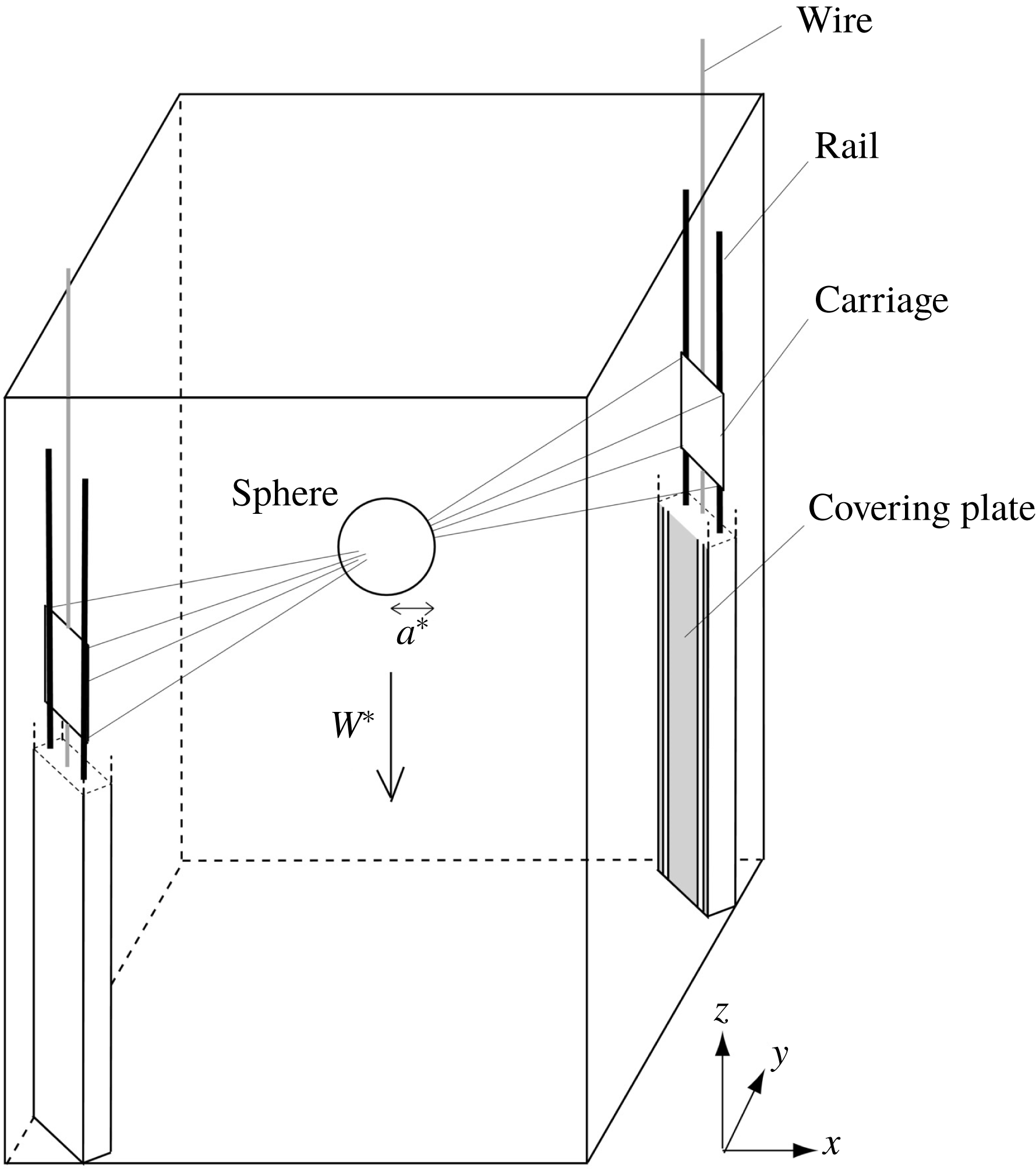
An acrylic sphere of radius
 $a^{\ast }=2~\text{cm}$
or 2.5 cm is used, and it is suspended by eight stainless-steel wires which span obliquely across the tank. The sphere can move upwards and downwards, but the experiments are performed only when the sphere moves downwards. The constant speed of the sphere is assured by a brushless DC motor with a speed control system (Oriental motor BXS460A-50S-3). The wire is very thin with the diameter of 0.1 mm, so that it does not affect the fluid flow.
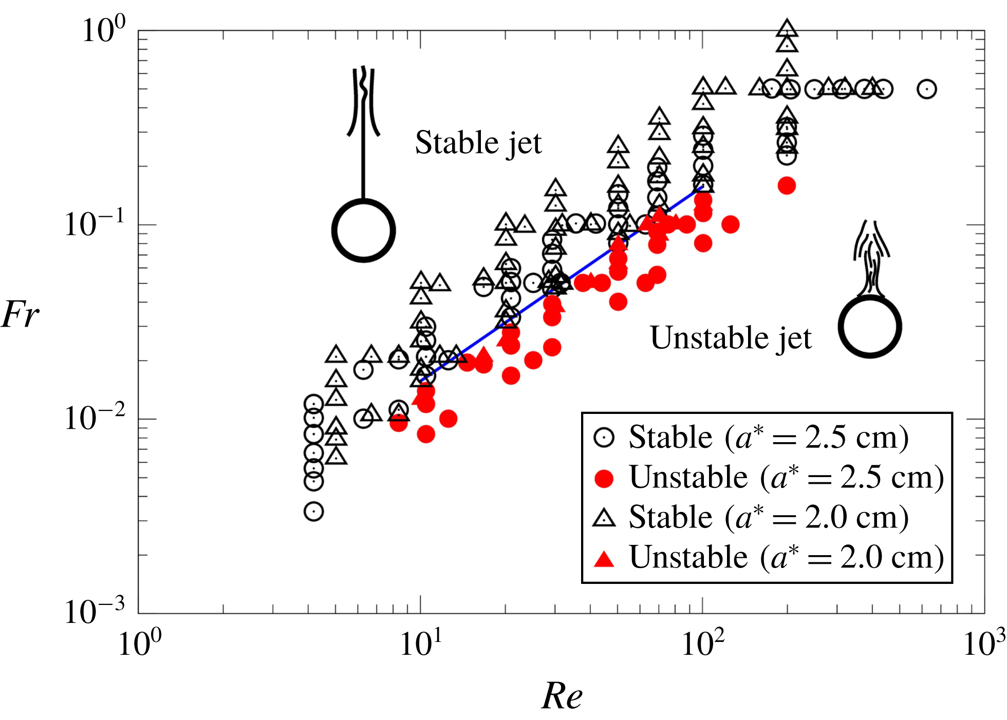
The parameter range (
 $Re,Fr$
) investigated in the present experiments. The open symbols denote stable jets, and the closed symbols denote unstable jets. The circles are the results for a large sphere (
 $a^{\ast }=2.5$
cm) and the triangles are the results for a small sphere (
 $a^{\ast }=2.0$
cm). The straight line of
 $Fr/Re=1.57\times 10^{-3}$
(
 $10\lesssim Re\lesssim 100$
) is the threshold line below which the jet becomes unstable.
The standard shadowgraph technique (Hanazaki et al.
Reference Hanazaki, Kashimoto and Okamura2009a
) is applied, using a 230 W ultra-high-pressure mercury lamp as light source. A translucent white acrylic sheet of 1 mm thickness is used as a screen to be photographed by a charge-coupled device (CCD) camera with the resolution of
 $2048~\text{pixel}\times 2048~\text{pixel}$
(HiSense 4MC, Dantec Dynamics; C9300-024, Hamamatsu Photonics; 12 bits, 11 Hz) or by a digital single-lens reflex camera with
 $4256~\text{pixel}\times 2832~\text{pixel}$
(Nikon D3s).
Planar particle image velocimetry (PIV) is performed to measure the velocity in the vertical plane using the same apparatus as in the previous papers (Hanazaki et al.
Reference Hanazaki, Kashimoto and Okamura2009a
; Okino et al.
Reference Okino, Akiyama and Hanazaki2017). The vertical light sheet is generated using a double-pulsed Nd:YAG laser (Dual Power 65-15, Dantec Dynamics; Nano S PIV, Litron Lasers; 532 nm, 65 mJ, 15 Hz), and images of the seeding particles are photographed by a CCD camera with
 $2048~\text{pixel}\times 2048~\text{pixel}$
(HiSense 4MC, Dantec Dynamics; C9300-024, Hamamatsu Photonics; 12 bits, 11 Hz). The parameters used for PIV are listed in table 1.
The list of parameters used for PIV. The Reynolds number is fixed at
 $Re=50$
, with the sphere diameter of 5 cm and sphere velocity of
 $W^{\ast }=0.1~\text{cm}~\text{s}^{-1}$
. A lens of long focal length (AI Micro-Nikkor 105 mm
 $f/\text{2.8S}$
) is used to obtain a high resolution. The alphabetic suffix (a–d) in the data name denotes the cases with different velocity distributions, obtained for the same
 $Fr$
and
 $Re$
.

Refractive-index matching (e.g. McDougall Reference McDougall1979) is not used in the present PIV so that the shadowgraph method which requires the inhomogeneity of refractive index can be performed in the same fluid. The change of refractive index in the vertical direction due to salt stratification can be estimated as follows. When the concentration of salt is
 $x^{\ast }~\text{g}~\text{l}^{-1}$
, the refractive index
 $n$
of salt water at
 $21\,^{\circ }\text{C}$
is (e.g. Daviero, Roberts & Maile Reference Daviero, Roberts and Maile2001)
 $$\begin{eqnarray}n=1.3329+1.71\times 10^{-4}x^{\ast }.\end{eqnarray}$$
Using the largest value of
 $N^{\ast }$
(
 $=1.0~\text{s}^{-1}$
) and the maximum vertical movement of the sphere (
 ${\sim}70$
cm) in the present experiment, the maximum variation of
 $x^{\ast }$
can be estimated as
 $\unicode[STIX]{x0394}x^{\ast }\sim 71.4~\text{g}~\text{l}^{-1}$
. Then, the corresponding variation in the refractive index is
 $\unicode[STIX]{x0394}n\sim 0.0122$
, giving a relative error (
 $\unicode[STIX]{x0394}n/n$
) of 0.92 %. This would give an estimate for the maximum error in the vertical position and the vertical velocity of seeding particles in PIV, when the density variation is gradual. In the present experiment when the Froude number is small (cf. figure 11 of Hanazaki et al.
Reference Hanazaki, Nakamura and Yoshikawa2015), the sphere drags down the upper fluid only for a small distance, and the actual variation of the refractive index would be much smaller. For example, when
 $Fr\leqslant 0.14$
, as in the present study, the dragged distance might be less than a few times the sphere diameter (
 ${\sim}15$
cm), giving a maximum relative error less than 0.2 %.
While the above estimates would give the overall errors, density contours might have a large curvature if the flow is turbulent with small-scale fluctuations. Then, the possibility should be considered that the deflection angle of the laser light becomes large in a short distance, leading to a larger local error. Meanwhile, due to the diffusion effects of salinity, a large discontinuity of the refractive index would not occur frequently in continuously stratified fluid, avoiding an abrupt deflection of light in a short distance. The density change along the horizontal light path in the
 $x$
direction would become largest very near the vertical axis (
 $x=y=0$
) passing through the centre of the sphere, where the density contours are approximately vertical. But the area with large density variation is narrow, comparable to the thickness of the density boundary layer on the sphere surface, which is estimated by
 $l_{\unicode[STIX]{x1D705}}^{\ast }/2a^{\ast }=\sqrt{Fr/(2\,Sc\,Re)}$
, where
 $Sc$
is the Schmidt number (see below). This has been confirmed by numerical simulations (Hanazaki et al.
Reference Hanazaki, Nakamura and Yoshikawa2015) for laminar flow, and in the present experiment the value becomes
 $l_{\unicode[STIX]{x1D705}}^{\ast }/2a^{\ast }=\sqrt{Fr/(2\,Sc\,Re)}=\sqrt{0.05/(2\times 700\times 50)}=8.5\times 10^{-4}$
. This is even smaller than the smallest resolved scale in PIV (127 data points in 4.5 cm (
 $=0.9\times 2a^{\ast }$
), so that the resolved scale is
 $0.9/127=7.0\times 10^{-3}$
), meaning that the refraction of light near the very centre of the jet would be hardly captured in the present PIV, and would not affect the measured velocity. We should note that, when the jet is just meandering, the region with density anomaly would be comparable to this estimate. When the jet is turbulent, the jet becomes much broader (figure 6
c), but the local density variation would be reduced due to the fluid mixing.
To confirm that refraction of light does not affect the velocity measurement significantly, we have performed an additional experiment with refractive-index matching, using ethanol. The results for the case of
 $Fr=0.044$
and
 $Re=50$
showed that the appearance ratio of error vectors is as low as the results without refractive-index matching, which gave a ratio generally less than 5 %.
Two objective lenses with different focal length (AI Micro-Nikkor 105 mm
 $f/\text{2.8S}$
and Nikkor 50 mm
 $f/1.2$
) are used. When we observe a large area above the sphere by the shadowgraph method, we have used the lens of short focal length (
 $=50$
mm) with a large angle of view (figures 3
a–c and 5), but otherwise we have used the micro lens of longer focal length (
 $=105$
mm) with a smaller angle of view to achieve higher resolution.
The governing parameters of the flow are the Froude number, Reynolds number and Schmidt number, but the Schmidt number
 $Sc~(=\unicode[STIX]{x1D708}^{\ast }/\unicode[STIX]{x1D705}^{\ast })$
(with
 $\unicode[STIX]{x1D705}^{\ast }$
the diffusion coefficient of salinity) is constant since we use only salinity (
 $Sc\sim 700$
) to generate the stratified fluid. All the physical quantities are non-dimensionalised using the diameter of the sphere
 $2a^{\ast }$
, the constant downward velocity of the sphere
 $W^{\ast }$
and the vertical mean-density variation
 $-2a^{\ast }\text{d}\bar{\unicode[STIX]{x1D70C}^{\ast }}/\text{d}z^{\ast }$
as the density scale.
The sphere velocity
 $W^{\ast }$
and the Brunt–Väisälä frequency
 $N^{\ast }$
are varied in the range of
 $0.0084~\text{cm}~\text{s}^{-1}\leqslant W^{\ast }\leqslant 1.25~\text{cm}~\text{s}^{-1}$
and
 $0.25~\text{s}^{-1}\leqslant N^{\ast }\leqslant 1.0~\text{s}^{-1}$
along with the two values of
 $a^{\ast }$
(
 $=2.0$
cm and 2.5 cm), so that the Froude number (
 $Fr=W^{\ast }/N^{\ast }a^{\ast }$
) and the Reynolds number (
 $Re=W^{\ast }(2a^{\ast })/\unicode[STIX]{x1D708}^{\ast }$
) are varied in the range of
 $0.003\leqslant Fr\leqslant 1$
and
 $4\leqslant Re\leqslant 600$
. The parameter range investigated in this study is presented in figure 2.
The blue straight line in figure 2 is the threshold line between the stable jet and the unstable jet. The line represents
 $$\begin{eqnarray}Fr/Re=1.57\times 10^{-3}\quad (10\lesssim Re\lesssim 100),\end{eqnarray}$$
and the jet becomes unstable below this line (
 $Fr/Re<1.57\times 10^{-3}$
).
There are two unstable states. When the originally axisymmetric jet first becomes unstable, a meandering jet appears, but if the flow becomes more unstable, the jet becomes turbulent. When the ratio
 $Fr/Re$
is not much less than
 $1.57\times 10^{-3}$
and the instability is not strong, a transition region exists, and both the meandering jet and the turbulent jet can be observed at the same parameters (
 $Fr$
and
 $Re$
) depending on each realisation. When the ratio is sufficiently below the threshold value, the flow becomes turbulent immediately. More details will be discussed in § 3.
Only two sphere sizes (
 $a^{\ast }=2.0$
and 2.5 cm) are used in this study, while a wide range of variation of
 $a^{\ast }$
is preferable to confirm that the relation (2.2) holds independent of the sphere size. However, usage of a sphere of smaller size means a smaller observation area and smaller-scale structures, often leading to less resolution. Therefore, we use in this study a sphere whose radius is no less than
 $a^{\ast }=2$
cm. On the other hand, the maximum attainable time in the present experiment is
 $W^{\ast }t_{max}^{\ast }/2a^{\ast }=H^{\ast }/2a^{\ast }$
, where
 $H^{\ast }=W^{\ast }t_{max}^{\ast }=70$
cm is the vertical moving range of the sphere. Then, the maximum time becomes
 $H^{\ast }/2a^{\ast }=17.5$
when
 $a^{\ast }=2$
cm, and
 $H^{\ast }/2a^{\ast }=14$
when
 $a^{\ast }=2.5$
cm. Use of a larger radius of the sphere, for example
 $a^{\ast }=3$
cm, gives only
 $H^{\ast }/2a^{\ast }=11.7$
. This means that the observation in the time range of
 $W^{\ast }t^{\ast }/2a^{\ast }>10$
, i.e. after a stationary state is realised, becomes difficult for a sphere radius larger than 2.5 cm. The difference between
 $a^{\ast }=2$
and 2.5 cm is not large, but it makes the difference in
 $Fr/Re~(=\unicode[STIX]{x1D708}^{\ast }/(2N^{\ast }a^{\ast 2}))$
by
 $(2.5/2)^{2}~(=1.56)$
times. This has the same effect as the increase of
 $N^{\ast }$
by 1.56 times. Then, the variation of
 $a^{\ast }$
in this study would not be too small to be effective.
In presenting the results of this study, the origin of coordinates is at the centre of the sphere and the coordinate frame moves downwards with the sphere. The light propagates in the positive
 $x$
direction, and the
 $z$
axis is in the vertical direction (figure 1). The non-dimensional vertical velocity in the laboratory frame
 $w-1=(w^{\ast }-W^{\ast })/W^{\ast }$
is often used instead of the velocity relative to the sphere
 $w~(=w^{\ast }/W^{\ast })$
, since the velocity is directly measured in the laboratory frame.
The observation has been made after the flow has become stationary, and the data at non-dimensional time
 $t~(=W^{\ast }t^{\ast }/2a^{\ast })\gtrsim 10$
are used unless otherwise stated. We should note that the previous numerical simulations for axisymmetric flows have shown that the flow becomes steady earlier at lower Froude numbers (Hanazaki et al.
Reference Hanazaki, Nakamura and Yoshikawa2015). For example, at
 $Fr=1$
(
 $Re=200$
), the density at the upper stagnation point of the sphere becomes constant at
 $t\sim 10$
, while at
 $Fr=0.3$
, the density becomes constant at
 $t\sim 5$
. In this study, the Froude number is less than unity, and
 $Fr<0.3$
is satisfied in most of the cases. Then, the flows in this study would fully develop their axisymmetric aspects before
 $t=10$
.
3 Results
We first show the shadowgraph images in figure 3, where the Froude number is decreased from 0.12 to 0.04, while the Reynolds number is fixed at 50. When the Froude number is
 $Fr=0.12$
(figure 3
a), the flow pattern is similar to the one previously observed at
 $Fr=0.3$
or larger (cf. figure 5a of Hanazaki et al. (Reference Hanazaki, Kashimoto and Okamura2009a
), where
 $Fr=0.32$
and
 $Re=199$
). Namely, the pattern is characterised by a straight thin jet surrounded by a bell-shaped structure which has been named ‘type A’ in Hanazaki et al. (Reference Hanazaki, Kashimoto and Okamura2009a
). The vertical distance of the bell-shaped structure from the sphere is proportional to the Froude number since the bell is generated by the downward flow due to internal gravity waves, and the vertical wavelength determines the position of the bell (Hanazaki et al.
Reference Hanazaki, Nakamura and Yoshikawa2015).
Jet structures observed by shadowgraph (
 $Re=50$
): (a)
 $Fr=0.12$
(
 $Fr/Re=2.4\times 10^{-3}$
); (b)
 $Fr=0.080$
(
 $Fr/Re=1.6\times 10^{-3}$
); (c)
 $Fr=0.067$
(
 $Fr/Re=1.34\times 10^{-3}$
); (d)
 $Fr=0.057$
(
 $Fr/Re=1.14\times 10^{-3}$
); and (e)
 $Fr=0.040$
(
 $Fr/Re=0.8\times 10^{-3}$
).

As the Froude number decreases, the height of the bell-shaped structure decreases, and the instability of the jet appears at low Froude numbers (
 $Fr\leqslant 0.067$
and
 $Fr/Re\leqslant 1.34\times 10^{-3}$
; cf. (2.2)). At the same time, the jet becomes broad since the multiple black lines with negative density anomaly originate from a wider region around the upper stagnation point of the sphere. The unstable jet becomes turbulent and shows small-scale structures at some height from the sphere (
 $z\gtrsim 0.9$
). In the case of lowest
 $Fr~(=0.04)$
, small-scale turbulence appears even near the upper stagnation point of the sphere.
We should note that an unstable jet appears at the Reynolds number of 50, for which the flow is steady and axisymmetric in homogeneous fluid. The unstable jet actually appears at Reynolds numbers as low as 10. In figure 4(a), an unstable jet appears at
 $Re=20$
with a Froude number lower than in figure 3 (
 $Fr=0.016$
), and in figure 4(b) an unstable jet appears even at
 $Re=10$
, with a further lower Froude number of 0.008. The unstable jet may even appear at lower
 $Re$
if the Froude number is lower (cf. figure 2).
Unstable jets visualised by shadowgraph at low Reynolds numbers: (a)
 $Fr=0.016$
,
 $Re=20$
(
 $Fr/Re=0.8\times 10^{-3}$
); and (b)
 $Fr=0.008$
,
 $Re=10$
(
 $Fr/Re=0.8\times 10^{-3}$
).

The straight threshold line in figure 2 ends at
 $Re=10$
and
 $Fr=0.0157$
. The clear identification of instability becomes increasingly difficult at lower
 $Re$
and
 $Fr$
, since the turbulent fluctuations become weak at low
 $Re$
, and the length of the jet becomes short at low
 $Fr$
, making the unstable jets difficult to discern. In addition, the vertically dragged length of the fluid by the sphere decreases in proportion to
 $Fr$
(Hanazaki et al.
Reference Hanazaki, Nakamura and Yoshikawa2015), making a smaller density difference between the jet and the surrounding fluid. Then, the black and white contrast in the shadowgraph would become weaker. We could identify, however, that the threshold line deflects downwards beyond this left end point, i.e. the jet at some
 $Re({\leqslant}10)$
remains stable for lower
 $Fr$
, probably because the dissipation due to viscosity becomes more significant than the destabilising effect of stratification.
The straight threshold line has the other end at
 $Re=100$
and
 $Fr=0.157$
, beyond which the inclination of the line becomes small, and the jet becomes stable for
 $Fr/Re<1.57\times 10^{-3}$
. For example, at
 $Re=200$
, the jet is stable for moderately strong stratification (
 $Fr\sim 0.2$
), similarly to the previous experiments for a larger
 $Fr~(=0.3)$
(Hanazaki et al.
Reference Hanazaki, Kashimoto and Okamura2009a
).
Instability of the jet can occur in a short time after the sphere begins to move. The time development for
 $Fr=0.057$
and
 $Re=50$
(figure 3
d) is presented in figure 5. For an initial short period (
 $t\lesssim 1$
), an axisymmetric jet with a bell-shaped structure is generated (figure 5
a). This initial pattern would have been maintained if the flow had been stable. At
 $t=1.0$
(figure 5
b), however, the jet begins to meander, and at
 $t=1.1$
(figure 5
c), several new plumes (black lines) appear near the original jet, indicating the additional low-density anomaly which leads to the transition to turbulence. At
 $t=1.75$
(figure 5
d), the jet becomes turbulent and the pattern is already very similar to figure 3(d) observed much later (
 $t\gtrsim 10$
). We should note here that, while the flow becomes turbulent (figure 5
d) in some realisations, it remains just meandering (figure 5
b) for a long time (
 $t\gtrsim 10$
) in other realisations. Therefore, there are two different states for the same set of parameters (
 $Fr=0.057$
and
 $Re=50$
). The multiple states would be observed near the transition parameters, which satisfy
 $Fr/Re<1.57\times 10^{-3}$
. In the present case,
 $Fr/Re=1.14\times 10^{-3}$
. The appearance of meandering state or turbulent state will be further discussed below.
Generation process of an unstable jet visualised by shadowgraph, with
 $Fr=0.057$
,
 $Re=50$
 $(Fr/Re=1.14\times 10^{-3})$
: (a)
 $t=0.75$
, (b)
 $t=1.0$
, (c)
 $t=1.1$
, and (d)
 $t=1.75$
.
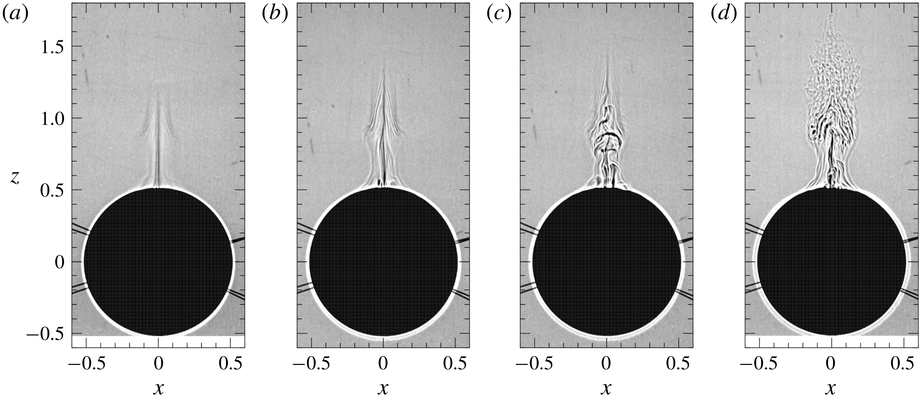
Figure 6 shows the developed velocity distributions (
 $t>10$
) observed by PIV in the vertical (
 $x{-}z$
) plane across the centre of the sphere. The Reynolds number is fixed at
 $Re=50$
, while the Froude number decreases from left to right. In all panels, the region of large vertical velocity, i.e. a ‘jet’, is identified by the upward vectors near the
 $z$
axis.
We note that figures 6(b,c) are the results for the same Froude number (
 $Fr=0.057$
) but show different patterns. These two states appear near the threshold Froude number which separates the stable and unstable states. Figure 6(b) shows the meandering jet (cf. figure 5
b), while figure 6(c) shows the turbulent jet (figure 5
d).
It is difficult to determine the condition whether the jet remains just meandering or becomes turbulent, but it would probably depend on the strength of the environmental disturbances of velocity and density which exist initially in the test tank. The instability of an axisymmetric jet makes a meandering jet in a short time (
 $t\sim 1$
) as observed in figure 5, but if the disturbance in the test tank is small, the jet remains just meandering (figures 5
b, 6
b and also 7
a), while it becomes turbulent if the disturbance is large enough (figures 5
d, 6
c and 7
b).
Velocity in the laboratory frame (
 $u,w-1$
) observed by PIV (
 $Re=50$
) in the vertical (
 $x{-}z$
) plane across the centre of the sphere. Blue lines show the contours of zero vertical velocity (
 $w-1=0$
). Panel (a) is made by vertically connecting the two velocity fields observed at different instants (
 $t=W^{\ast }t^{\ast }/2a^{\ast }=10.5$
and 11.4), using the steadiness of the flow to constitute an image of a vertically long region. Each field covers the vertical range of
 $0.48\leqslant z\leqslant 1.34$
and
 $1.38\leqslant z\leqslant 2.25$
, respectively. Panels (b–d) show the instantaneous velocities at
 $t\simeq 10.5$
. The velocity vectors obtained by PIV are plotted for only every fourth point in both the horizontal and vertical directions to avoid the overlap of vectors. The downward arrow at the centre of the sphere indicates five times the velocity of the descending sphere. Cases: (a) [Fr0.12]
 $(Fr/Re=2.4\times 10^{-3})$
; (b) [Fr0.057a]
 $(Fr/Re=1.14\times 10^{-3})$
; (c) [Fr0.057b]
 $(Fr/Re=1.14\times 10^{-3})$
; and (d) [Fr0.040]
 $(Fr/Re=0.8\times 10^{-3})$
.

To look at the details of the velocity distribution, close-up views of figure 6(b,c) are shown in figure 7(a,b), respectively. We clearly observe a meandering jet in figure 7(a), while the turbulent jet in figure 7(b) shows a weaker asymmetry. The comparatively weak asymmetry in figure 7(b) is due to the generally small horizontal velocity components, although the vertical components have an asymmetric distribution (cf. figure 8 c,d).
We may also note the difference between the shadowgraph and the PIV results. The small-scale structures of salt/density diffusion (
 $\unicode[STIX]{x1D6FB}^{2}\unicode[STIX]{x1D70C}$
) generated by the high Schmidt number of salt (
 ${\sim}700$
) would be resolved only by the shadowgraph (e.g. 2048 pixel
 $\times$
2048 pixel for
 $11~\text{cm}\times 11~\text{cm}$
in figure 3
e). On the other hand, the velocity distribution would not have these small-scale structures, contributing also to an apparently weaker asymmetry in figure 7(b).
In figures 6 and 7, the typical diverging internal wave patterns can be identified by the blue lines which show the contours of zero vertical velocity in the laboratory frame. The vertical distance between the blue lines, which corresponds to the half wavelength of the internal wave, decreases with the Froude number. When the jet is turbulent at low Froude numbers (figures 6
c, 6
d and 7
b), the blue lines of zero vertical velocity horizontally pass through the
 $z$
axis, and upward and downward velocity appear alternately in the vertical direction. This has not been observed at higher Froude numbers (figure 6
a) where stronger jets have been observed. When the jet becomes turbulent, the fluid in the jet mixes with the surrounding fluid, and the density difference between the jet and the surrounding fluid becomes smaller. Then, the buoyancy effect and hence the vertical velocity in the jet become smaller, leading to the appearance of the internal wave effects on the symmetry axis.
Close-up views of (a) figure 6(b) and (b) figure 6(c) (
 $Fr=0.057,Re=50$
). The velocity vectors are plotted for every third point in the vertical direction to avoid the overlap of vectors, while all the measured vectors are plotted in the horizontal direction. The downward arrow inside the sphere indicates five times the velocity of the descending sphere.
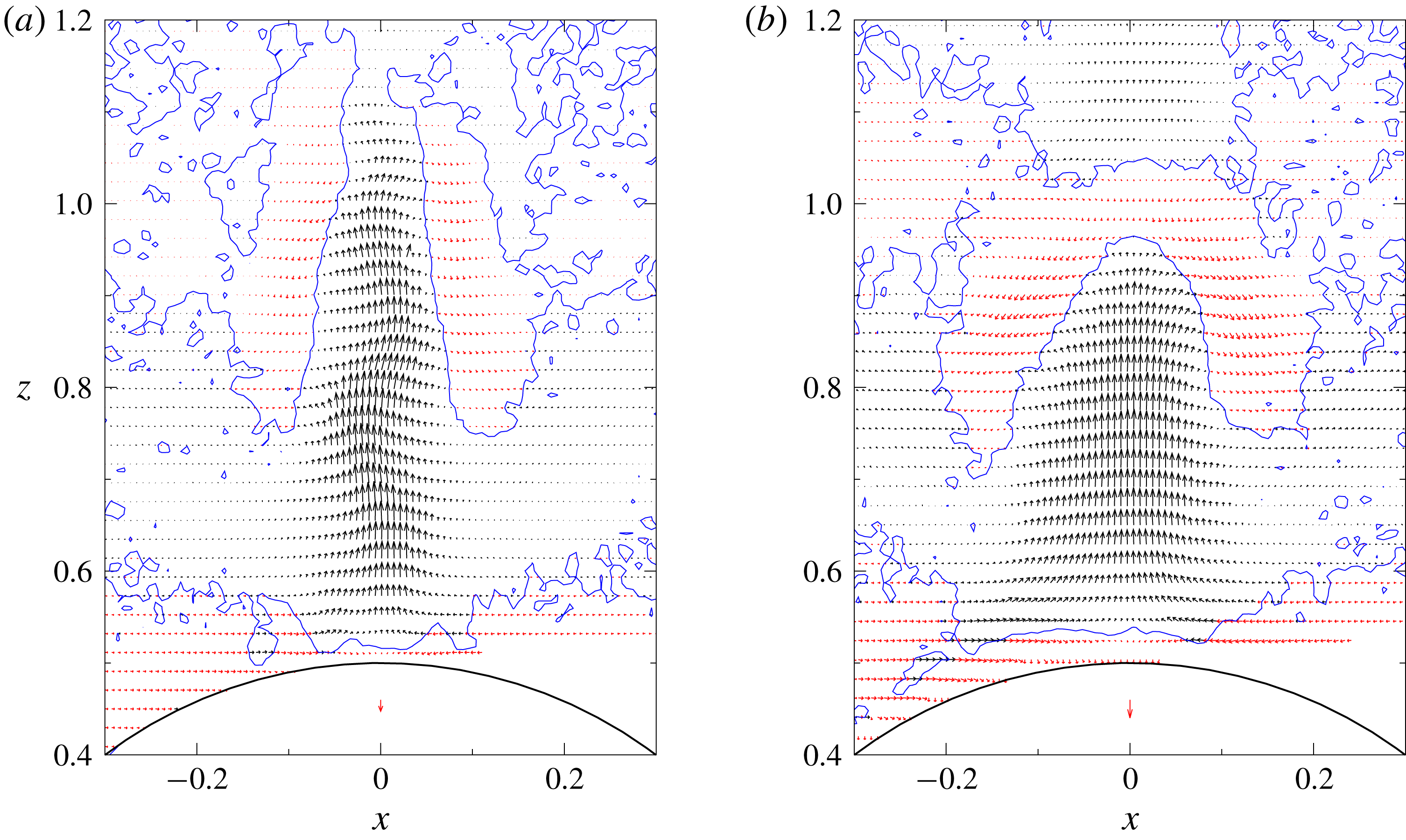
Figure 8 shows the typical contours of vertical velocity for the meandering jet (figure 8
a,b) and the turbulent jet (figure 8
c,d), again observed when
 $Fr=0.057$
and
 $Re=50$
.
Time dependence of the vertical velocity when the jet is unstable (
 $Fr=0.057$
,
 $Re=50$
), i.e.
 $Fr/Re=1.14\times 10^{-3}<1.57\times 10^{-3}$
. The velocity in the laboratory frame (
 $w-1$
) measured by PIV in the vertical (
 $x{-}z$
) plane is depicted in colour maps, using the same data as in figure 6(b,c), but at slightly different times. The upper row shows the meandering jet [Fr0.057a] at (a)
 $t=10.37$
and (b)
 $t=10.39$
, and the lower row shows the turbulent jet [Fr0.057b] at (c)
 $t=10.55$
and (d)
 $t=10.57$
. The time difference is
 $\unicode[STIX]{x0394}t=0.02$
in both jets. The bold (blue) lines are the contours of zero vertical velocity (
 $w-1=0$
), and the thin (black) solid and dotted lines denote the positive and negative vertical velocity respectively, at the contour interval of
 $\unicode[STIX]{x0394}(w-1)=1$
.

When the jet is meandering, temporally quasi-periodic oscillations travel upwards along the jet at a nearly constant speed, and figure 8(a,b) shows the velocity distributions at the opposite phase. Since the non-dimensional time difference is 0.02, the oscillation period
 $T^{\ast }$
is given by
 $W^{\ast }T^{\ast }/2a^{\ast }=0.02\times 2=0.04$
. In the buoyancy oscillation in stratified fluids, the maximum possible frequency is the Brunt–Väisälä frequency
 $N^{\ast }$
. Then, the Brunt–Väisälä period
 $2\unicode[STIX]{x03C0}/N^{\ast }$
is the shortest period
 $T_{min}^{\ast }=2\unicode[STIX]{x03C0}/N^{\ast }$
, which can be rewritten as
 $$\begin{eqnarray}W^{\ast }T_{min}^{\ast }/2a^{\ast }=\unicode[STIX]{x03C0}Fr.\end{eqnarray}$$
In the present case (
 $Fr=0.057$
), the Brunt–Väisälä period is
 $\unicode[STIX]{x03C0}Fr=0.18$
, and the observed period (
 $=0.04$
) is much shorter than this value, suggesting that the observed oscillation does not have its origin in buoyancy or internal waves.
When the jet is turbulent (figures 8
c,d), the asymmetry looks weaker, but it exists as observed in figure 7(b). The unsteadiness is less significant since the time-averaged component of the jet is much larger than the fluctuating component, and the temporal variation of vertical velocity is generally less than 10 %. We could still reveal that the position of the largest vertical velocity ascends periodically, by examining the temporal evolution of velocity in a short time interval of
 $\unicode[STIX]{x0394}t\simeq 5\times 10^{-3}$
. The fluctuating or ‘turbulent’ components of velocity would exchange energy with the density fluctuations through the vertical density flux, and the fluctuation in density can be observed in the shadowgraph (figures 3
d and 5
d). Even smaller-scale fluctuations of density can be observed due to the high Schmidt number of salinity (
 $Sc\sim 700$
).
Figure 9 shows the distributions of vertical velocity on the
 $z$
axis. As the Froude number decreases from 0.12 to 0.04, the maximum velocity on the
 $z$
axis, i.e.
 $w_{max}-1$
, first increases until
 $Fr=0.08$
, but it decreases below
 $Fr=0.08$
(probably between
 $Fr=0.08$
and 0.067, cf. figure 3
b,c). In the meandering state [Fr0.057a] the jet is unstable but still thin, so that the vertical velocity is as high as the case of
 $Fr=0.08$
. If the meandering jet evolves into a turbulent jet [Fr0.057b], the maximum velocity significantly decreases and becomes small. As the Froude number decreases further down to
 $Fr=0.04$
, the velocity increases again.
In figure 9, the vertical velocity at low Froude numbers (
 $Fr\leqslant 0.057$
) changes sign along the
 $z$
axis, and regions of
 $w-1>0$
and
 $w-1<0$
appear alternately. This is due to the internal waves which could be observed in figure 6. The first zero of
 $w-1=0$
on the
 $z$
axis moves downwards as the Froude number decreases, corresponding to the decreased wavelength of the internal wave.
Distribution of the vertical velocity in the laboratory frame (
 $w-1$
) on the
 $z$
axis observed by PIV (
 $0.04\leqslant Fr\leqslant 0.12$
,
 $Re=50$
). The origin of coordinates is at the centre of the sphere, and
 $z=0.5$
is the upper stagnation point of the sphere.
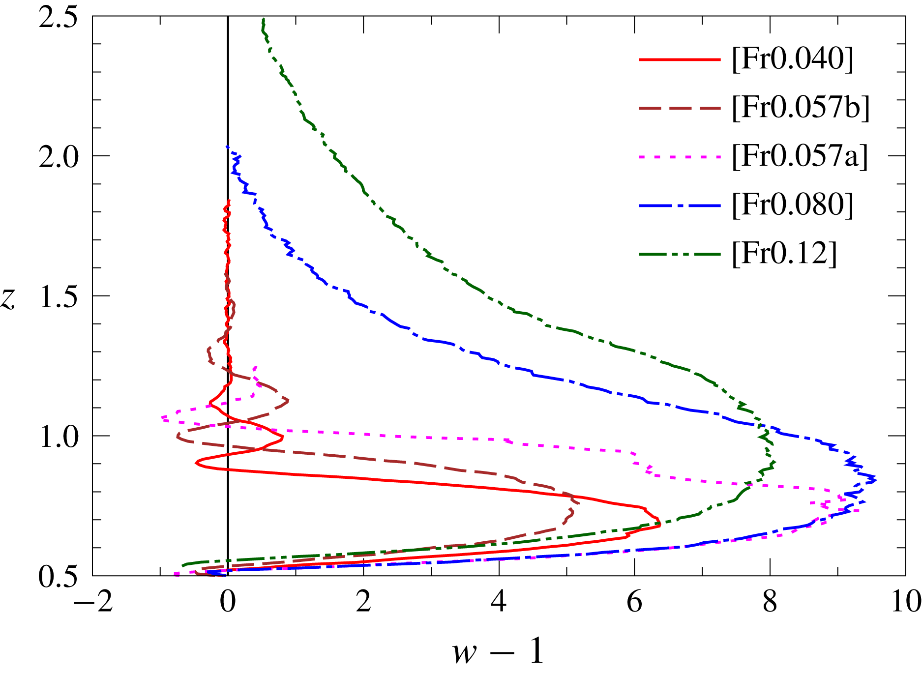
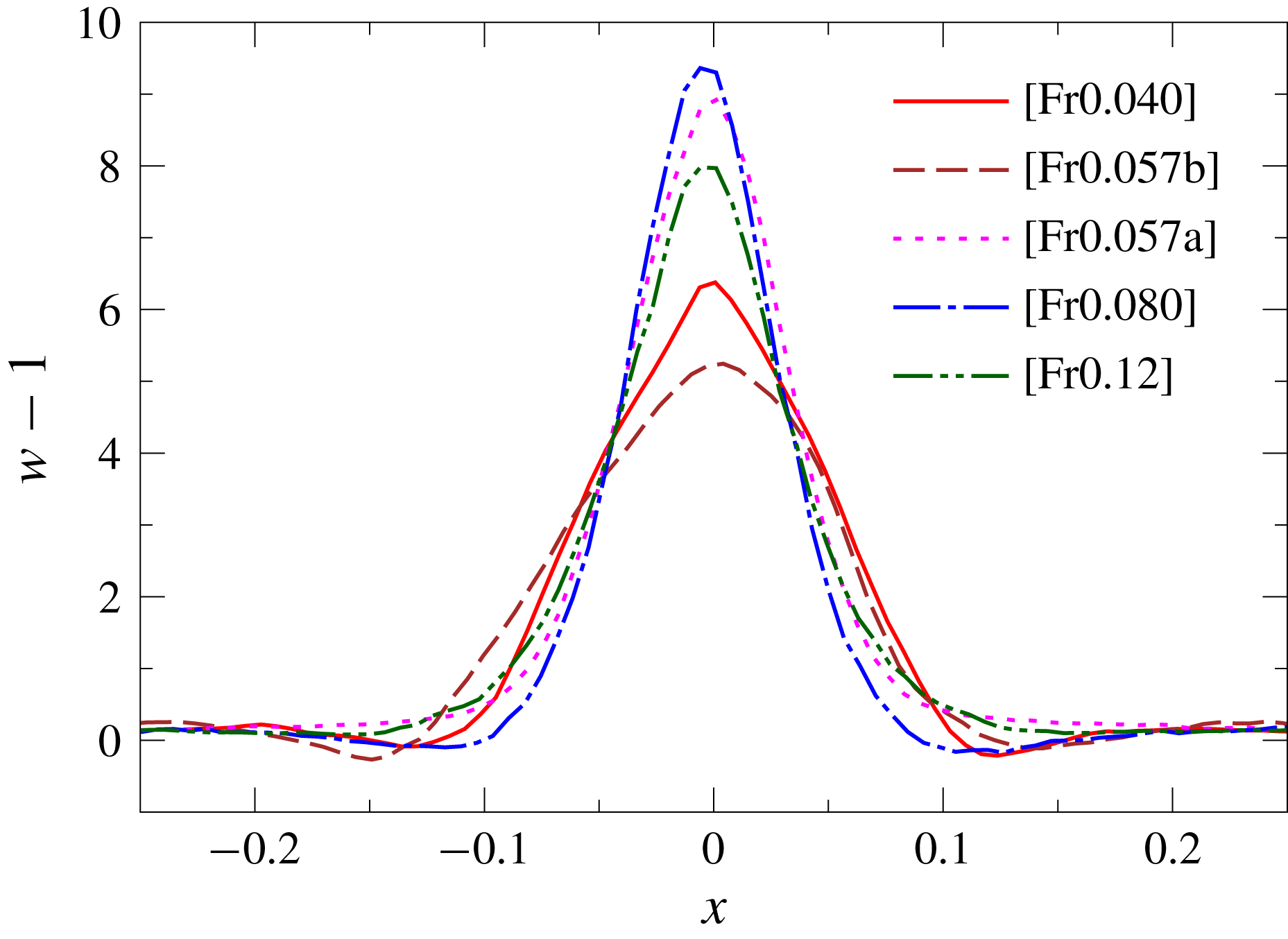
Figure 10 shows the horizontal distribution of the time-averaged vertical velocity at the height of maximum vertical velocity
 $z_{w_{max}}$
. As the Froude number decreases from 0.12 to 0.08, the jet becomes faster while it becomes thinner in agreement with figure 9, and the jet remains fast even when the jet becomes unstable at
 $Fr=0.057$
, as long as the jet is just meandering and still thin [Fr0.057a]. However, when the instability develops and the jet becomes turbulent, the mean vertical velocity of the jet decreases suddenly [Fr0.057b]. When
 $Fr$
decreases further (
 $Fr=0.04$
), the jet becomes faster again, probably due to the increased buoyancy at the low Froude number.
Distribution of the time-averaged vertical velocity on the horizontal line located at the height of maximum vertical velocity (
 $z=z_{w_{max}}$
and
 $y=0$
). Observation by PIV for
 $0.04\leqslant Fr\leqslant 0.12$
and
 $Re=50$
.
Maximum vertical velocity in the jet
 $w_{max}-1$
observed by PIV for
 $Fr=0.04$
, 0.05, 0.057, 0.067, 0.08, 0.10, 0.12 and 0.14 (
 $Re=50$
). Time-averaged values of
 $w_{max}-1$
are denoted by the symbols. The error bar shows the standard deviation from the time-averaged value in each realisation. The vertical dashed line denotes the stability boundary determined from the shadowgraph experiments, i.e.
 $Fr=1.57\times 10^{-3}Re=0.0785$
or
 $1/Fr=12.7$
.
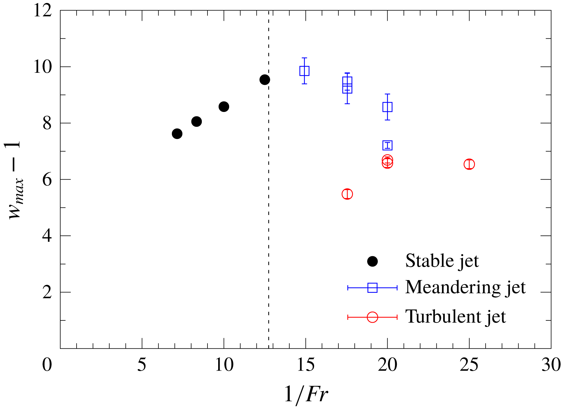
The maximum vertical velocity in the jet (
 $w_{max}-1$
) is plotted against
 $1/Fr$
in figure 11. We observe that the maximum velocity increases in proportion to
 $1/Fr$
for small
 $1/Fr$
(
 $0.08\leqslant Fr\leqslant 0.14$
), and reaches the maximum near
 $Fr=0.067$
(i.e.
 $1/Fr=15$
), for which the meandering jet appears and the instability begins (
 $Fr/Re=1.34\times 10^{-3}<1.57\times 10^{-3}$
).
For
 $Fr=0.057$
and 0.05 (i.e.
 $1/Fr=17.5$
and 20), two unstable states, i.e. the meandering jet and the turbulent jet, can appear for a single
 $Fr$
. The meandering jets denoted by open squares generally have faster velocities than the turbulent jets denoted by open circles if the value of
 $Fr$
is the same. The fluctuation defined by the standard deviation of the vertical velocity is larger in the meandering jet than in the turbulent jet. For example, the maximum velocity in the meandering jet [Fr0.057c] fluctuates in the range of
 $9.2\pm 0.5$
, while the velocity in the turbulent jet [Fr0.057b] fluctuates in the range of
 $5.5\pm 0.2$
.
As noted in figure 6, the appearance of either of the two states in the transition Froude numbers (
 $0.04\lesssim Fr\lesssim 0.067$
), i.e. the meandering jet or the turbulent jet, would depend sensitively on the initial small disturbances of velocity and density in the test tank, and it would be difficult to know a priori which of them appears, although a larger disturbance will usually lead to a turbulent jet. This would have some resemblance to the flow past a sphere, in which a trip wire on the sphere surface has been used to increase the disturbance in the upstream flow, helping the transition of a laminar boundary layer to a turbulent boundary layer (Van Dyke Reference Van Dyke1982). The existence of two possible states for the same parameter (Reynolds number) has been known also in the transition to turbulence in pipe flow (Darbyshire & Mullin Reference Darbyshire and Mullin1995).
The jet becomes narrower as the Froude number decreases from
 $Fr=0.14$
to 0.08 (cf. figure 10), while the vertical velocity increases (
 $(w_{max}-1)\propto 1/Fr$
). The proportionality of the jet radius to
 $Fr^{1/2}$
has been observed in previous studies for
 $0.3\leqslant Fr\lesssim 1$
(Hanazaki et al.
Reference Hanazaki, Nakamura and Yoshikawa2015; Okino et al.
Reference Okino, Akiyama and Hanazaki2017), where the radius has been estimated by the primitive length scale of the stratified fluid:
 $$\begin{eqnarray}l_{\unicode[STIX]{x1D708}}^{\ast }=\sqrt{\frac{\unicode[STIX]{x1D708}^{\ast }}{N^{\ast }}},\end{eqnarray}$$
which can be rewritten in non-dimensional form as
 $$\begin{eqnarray}\frac{l_{\unicode[STIX]{x1D708}}^{\ast }}{2a^{\ast }}=\sqrt{\frac{Fr}{2Re}}.\end{eqnarray}$$
These relations would be applied to the lower Froude numbers (
 $Fr<0.3$
) investigated in this study until the instability appears. For example, if we substitute
 $Fr=0.1$
and
 $Re=50$
into (3.3),
 $l_{\unicode[STIX]{x1D708}}^{\ast }/2a^{\ast }$
becomes
 $3.16\times 10^{-2}$
, which is quite comparable to the actually observed HWHM value of the velocity distribution in figure 10.
On the other hand, since close examination shows that the meandering at
 $Re=50$
begins between
 $Fr=0.078$
and 0.080, the threshold value of
 $Fr/Re$
is between
 $1.56\times 10^{-3}$
and
 $1.60\times 10^{-3}$
, in agreement with (2.2). Then, the combination of (3.3) with (2.2) gives
 $$\begin{eqnarray}l_{\unicode[STIX]{x1D708}}^{\ast }/2a^{\ast }=0.028\quad (10\lesssim Re\lesssim 100),\end{eqnarray}$$
as the minimum radius of a stable jet. This shows that the radius of the jet, which is estimated by the fundamental length scale of stratified fluid
 $l_{\unicode[STIX]{x1D708}}^{\ast }$
, cannot become narrower than 2.8 % of the sphere diameter
 $2a^{\ast }$
, in the range of
 $10\lesssim Re\lesssim 100$
.
The instability begins when the boundary-layer thickness, which is comparable to the jet radius, becomes thin (
 $=0.028\times 2a^{\ast }$
), and the velocity shear in the boundary layer becomes large enough for the onset of instability. Then, the generated disturbances would be transferred into the jet, and generate a meandering or turbulent jet. The minimum thickness is independent of
 $N^{\ast }$
, suggesting that the instability does not have its origin in the internal wave, in agreement with the discussions on the oscillation period of the jet (figure 8).
It would be of interest to note that
 $0.028\times 2a^{\ast }$
is equal to
 $2a^{\ast }/\sqrt{1275}$
, which is the boundary-layer thickness in a homogeneous fluid at
 $Re=1275$
. This value is not very different from the Reynolds number for which the vortex shedding from the sphere first appears, and may support the hypothesis that the boundary layer is the origin of instability.
We note that the radius of the jet discussed above is based on the velocity distribution, and the jet radius estimated by the density distribution might be much smaller, since it would be comparable to the density boundary-layer thickness on the sphere surface (Hanazaki et al.
Reference Hanazaki, Nakamura and Yoshikawa2015) estimated by
 $0.028/\sqrt{Sc}=1.06\times 10^{-3}$
(cf. (3.4) and Schmidt number of salt
 $Sc=700$
), or approximately 0.1 % of the sphere diameter. However, this expression shows at the same time that, for a fluid of much lower Schmidt or Prandtl number such as the thermally stratified water (
 $Pr=7$
), the jet radius defined by the density distribution would be 10 times larger. In this case, the radius based on the velocity distribution would also become slightly larger, as observed in the numerical simulation (Hanazaki, Konishi & Okamura Reference Hanazaki, Konishi and Okamura2009b
). Then, for a fluid of lower Schmidt number, a Froude number lower than (2.2) might be necessary for the onset of instability, although further investigation is necessary to confirm this prediction.
4 Conclusions
We have found unstable jets generated by a sphere descending in a very strongly stratified fluid (
 $Fr\lesssim 0.2$
). The threshold line for the instability is plotted again in figure 12 using the same data as in figure 2, but this time in
 $Re{-}Fr/Re$
coordinates to confirm that the threshold line becomes almost exactly horizontal. In the Reynolds-number range of
 $10\lesssim Re\lesssim 100$
, instability of the jet appears when the condition
 $Fr/Re<1.57\times 10^{-3}$
is satisfied. Since the boundary-layer thickness on the sphere surface and the radius of the jet are comparable to the primitive length scale of the stratified fluid
 $l_{\unicode[STIX]{x1D708}}^{\ast }/2a^{\ast }=\sqrt{Fr/2Re}$
, the condition predicts that the minimum radius of a stable jet is 2.8 % of the diameter of the sphere.
The threshold line for the instability, replotted using the same data as figure 2, but in
 $Re{-}Fr/Re$
coordinates to confirm that the threshold line (
 $Fr/Re=1.57\times 10^{-3}$
for
 $10\lesssim Re\lesssim 100$
) becomes horizontal.

The instability begins when the boundary-layer thickness becomes thin (
 ${\sim}0.028\times 2a^{\ast }$
), and the velocity shear in the boundary layer becomes large enough. Then, the disturbances generated by the shear instability would be transferred into the jet, generating an unstable jet.
When the flow is marginally unstable (e.g.
 $Fr=0.057$
,
 $Re=50$
and
 $Fr/Re=1.14\times 10^{-3}$
), two unstable states coexist. One is the meandering jet and the other is the turbulent jet. The meandering jet is thin, and its vertical velocity is as high as the stable axisymmetric jet observed for a slightly higher
 $Fr$
. On the other hand, the turbulent jet is broad due to the mixing with the surrounding fluid, and its vertical velocity becomes much smaller. In some cases, the meandering jet persists for a long time (
 $t\gtrsim 10$
), but in other cases, the meandering jet develops into a turbulent jet.
When the instability is sufficiently strong, i.e. when the value of
 $Fr/Re$
is significantly lower than
 $1.57\times 10^{-3}$
(e.g.
 $Fr=0.04$
,
 $Re=50$
and
 $Fr/Re=0.8\times 10^{-3}$
), the meandering jet does not appear and only the turbulent jet could be observed.
The instability would be observed also at lower Reynolds numbers (
 $Re<10$
), but only for
 $Fr$
somewhat smaller than the threshold value, which satisfies
 $Fr/Re=1.57\times 10^{-3}$
, since the stabilising effect of viscosity overcomes the destabilising effect of stratification.
On the other hand, at higher
 $Re~({>}100)$
(and
 $Fr\lesssim 0.2$
), the jet tends to be stable for
 $Fr$
somewhat lower than the threshold value, which satisfies
 $Fr/Re=1.57\times 10^{-3}$
. For example, at
 $Re=200$
, the jet is still stable for a relatively strong stratification (
 $Fr=0.2$
) which gives
 $Fr/Re=1.0\times 10^{-3}$
, and an axisymmetric jet is observed. This result would be explained by the stabilising effect of the stratification when it is moderately strong but not too strong.
Acknowledgement
This study was supported by JSPS KAKENHI grant nos. 24656124 and 15K17972.



