1. Introduction
The evolution of the number of individuals in a population and its genetic profile has been extensively studied. Two of the main families of processes used in this context are branching processes and frequency Wright–Fisher type processes, also known as two-type Fleming–Viot processes. The relationship between these two has been a formidable source of mathematical questions. Some remarkable results on this topic were presented in [Reference Birkner, Blath, Capaldo, Etheridge, Möhle, Schweinsberg and Wakolbinger3] and [Reference Etheridge and March10]. In [Reference Etheridge and March10], Etheridge and March relate these two families by conditioning a Dawson–Watanabe superprocess to have constant mass, thereby obtaining a Fleming–Viot superprocess. This technique reached a peak in [Reference Birkner, Blath, Capaldo, Etheridge, Möhle, Schweinsberg and Wakolbinger3], where the relationship was extended by showing that self-similar branching processes correspond to
 $\beta$
-coalescents.
In this paper, we study the relationship between two-type Feller diffusions with continuous immigration and the generalized structured Wright–Fisher type models known as the two-island model with mutation and selection [Reference Nath and Griffiths24].
Our approach to relating these prominent families of processes is different from that in [Reference Birkner, Blath, Capaldo, Etheridge, Möhle, Schweinsberg and Wakolbinger3] and is inspired by two seminal papers [Reference Gillespie14,Reference Gillespie15], where Gillespie introduced a method to model the competition between two types of individuals. His method relies heavily on the concept of culling. He begins with the assumption that each population evolves according to independent Feller diffusions, possibly with different distributions. At particular times, which we refer to as sampling times, the total population size is returned to a fixed level in such a way that the relative frequency of each type is preserved. It is important to note that the two competing populations are not assumed to have the same reproduction mechanism. This recurrent sampling was inspired by seasonal species and accurately describes the recurrent sampling characteristic of experimental evolution. The most prominent example of experimental evolution is the Lenski experiment [Reference Tenaillon28] (see [Reference González Casanova, Kurt, Wakolbinger and Yuan16] for a probabilistic approach to recurrent sampling experiments).
The Gillespie recurrent sampling method (GRSM) was mathematically formalized in [Reference Caballero, González Casanova and Pérez8] and extended to include jumps and immigration in the one-dimensional continuous-state branching process that models the population size of each type. The GRSM is less stringent than the time-change method in [Reference Birkner, Blath, Capaldo, Etheridge, Möhle, Schweinsberg and Wakolbinger3] since it relates branching and frequency processes only in distribution. However, it is more general; in particular, it can be applied to pairs of branching processes with different distributions, leading to asymmetric frequency processes.
In this paper, we extend the GRSM to the two-dimensional setting by applying this procedure to two-type Feller diffusions with immigration. The resulting family, which we call asymmetric two-island frequency processes, includes, as special cases, the seed bank model [Reference Blath, González Casanova, Kurt and Wilke-Berenguer5,Reference Blath, González Casanova, Kurt and Wilke-Berenguer6] and the two-island model [Reference Nath and Griffiths24]. The main strength of the two-dimensional GRSM is that it allows for comparing populations with different reproduction mechanisms, where each individual can be in one of two different states (e.g., active/dormant or island 1/island 2). Many members of this family have a genealogical structure in the sense of a moment dual. We will provide conditions for moment duality and describe the moment dual processes. This manuscript generalizes the work in [Reference Caballero, González Casanova and Pérez8] to the two-dimensional setting.
If we consider two-type branching processes consisting of active and dormant individuals, where active individuals can produce both active and dormant individuals, while dormant individuals can only activate, and apply the GRSM, we obtain the seed bank frequency processes with mutation and selection [Reference Blath, González Casanova, Kurt and Wilke-Berenguer5,Reference Blath, González Casanova, Kurt and Wilke-Berenguer6]. This connection between seed bank models and two-type branching processes is very natural. However, this appears to be the first time it has been formally established in the literature.
1.1. Two-type Feller diffusions with immigration
We start with a population consisting of two types of individuals, namely
 $\textbf{x}$
and
 $\textbf{y}$
, distributed between two islands, which we refer to as 1 and 2. The islands can be interpreted as two different states, for example dormant and active, or juvenile and mature individuals. We will assume that individuals can only give birth to offspring of the same type, but the offspring can reside on either of the two different islands. Additionally, we will consider external immigration events that contribute to the population of individuals of each type and island.
To this end, we consider that the population of individuals of type
 $\textbf{x}$
is described by a multitype Feller diffusion with immigration,
 $\textbf{X}\;:\!=\;\{\textbf{X}_t=(X^1_t,X^2_t)\colon t\geq 0\}$
, given as the unique strong solution to the following stochastic differential equation (SDE; see, for instance, [Reference Barczy, Li and Pap1]):
 \begin{equation*} \textbf{X}_t = \textbf{X}_0 + \int_0^t(\beta^X+B^X\textbf{X}_s)\,{\mathrm{d}} s + \sum_{i=1}^2\int_0^t\sqrt{c_i^XX_s^i}\,{\mathrm{d}} W_s^{X,i}e_i, \quad t\geq 0,\end{equation*}
where
 $\textbf{X}_0\;:\!=\;(x^1,x^2)\in\mathbb{R}_+^2$
,
 $\textbf{W}^X\;:\!=\;(W^{X,1},W^{X,2})$
is a two-dimensional Brownian motion,
 $e_1$
and
 $e_2$
denote the canonical vectors in
 $\mathbb{R}^2$
, and
 $c^X=(c_i^X)_{i\in\{1,2\}}\in\mathbb{R}_+^2$
,
 $\beta^X=(\beta_i^X)_{i\in\{1,2\}}\in\mathbb{R}_+^2$
, and
 $B^X=(B^X_{ij})_{i,j\in\{1,2\}}\in\mathbb{R}^{2\times2}_{(+)}$
, where
 $\mathbb{R}_+^2=[0,\infty)\times[0,\infty)$
and
 $\mathbb{R}^{2\times2}_{(+)}$
denotes the space of essentially non-negative
 $2\times2$
matrices, i.e. the set of matrices with non-negative off-diagonal entries.
Heuristically, the component
 $X^i$
describes the total mass of the population of individuals of type
 $\textbf{x}$
on island i for each
 $i=1,2$
. On the other hand, for each
 $i=1,2$
, the parameter
 $B^X_{ii}$
is related to the rate at which ‘infinitesimal individuals’ of type
 $\textbf{x}$
located on island i produce offspring of the same type on island i, while the variance associated with these branching events is denoted by
 $c_i^X$
. Additionally for
 $i,j=1,2$
with
 $i\not=j$
, the parameter
 $B^X_{ij}$
describes the rate at which ‘infinitesimal individuals’ of type
 $\textbf{x}$
residing on island j migrate to island i. Finally, the parameter
 $\beta^X_i$
depicts the rate at which immigration events occur that contribute to the total mass of the population of individuals of type
 $\textbf{x}$
on island i for each
 $i=1,2$
.
Similarly, the total mass of individuals of type
 $\textbf{y}$
is given by a multitype Feller diffusion with immigration,
 $\textbf{Y}\;:\!=\;\{\textbf{Y}_t=(Y^1_t,Y^2_t)\colon t\geq 0\}$
, defined as the unique strong solution to the following stochastic differential equation:
 \begin{equation} \textbf{Y}_t = \textbf{Y}_0 + \int_0^t(\beta^Y+B^Y\textbf{Y}_s)\,{\mathrm{d}} s + \sum_{i=1}^2\int_0^t\sqrt{c_i^YY_s^i}\,{\mathrm{d}} W_s^{Y,i}e_i, \quad t\geq 0,\end{equation}
where
 $\textbf{Y}_0\;:\!=\;(y^1,y^2)\in\mathbb{R}_+^2$
and
 $\textbf{W}^Y\;:\!=\;(W^{Y,1},W^{Y,2})$
is a two-dimensional Brownian motion independent from
 $\textbf{W}^X$
. Additionally,
 $c^Y=(c_i^Y)_{i\in\{1,2\}}\in\mathbb{R}_+^2$
,
 $\beta^Y=(\beta_i^Y)_{i\in\{1,2\}}\in\mathbb{R}_+^2$
, and
 $B^Y=(B^Y_{ij})_{i,j\in\{1,2\}}\in\mathbb{R}^{2\times2}_{(+)}$
. As in the case of individuals of type
 $\textbf{x}$
, the component
 $Y^i$
gives the total mass of individuals of type
 $\textbf{y}$
on island i for
 $i=1,2$
. The description of the parameters appearing in (1.1) is analogous to those of the process
 $\textbf{X}$
.
We remark that the two-type Feller diffusions discussed in this section can be obtained as rescaling limits in space and time of two-type Galton–Watson processes with immigration (see, for instance, [Reference Chunhua9]).
1.2. The asymmetric two-island frequency process
In this section we introduce a model for the relative frequency of individuals of type
 $\textbf{x}$
on two different islands under the assumption that the total mass on each island remains constant in time. We refer to this model as the asymmetric two-island frequency process. For
 $\textbf{z}=(z_1,z_2)\in(0,\infty)^2$
and
 $\textbf{r}=(r_1,r_2)\in[0,1]^2$
, we define the asymmetric two-island frequency process
 $\textbf{R}^{(\textbf{z},\textbf{r})}\;:\!=\;\big\{\textbf{R}^{(\textbf{z},\textbf{r})}_t=\big(R^{(\textbf{z},\textbf{r}),1}_t,R^{(\textbf{z},\textbf{r}),2}_t\big)\colon t\geq0\big\}$
as the solution of the stochastic differential equation
 \begin{align} & {\mathrm{d}}\textbf{R}^{(\textbf{z},\textbf{r})}_t \nonumber \\ & = b\big(\textbf{R}^{(\textbf{z},\textbf{r})}_t\big)\,{\mathrm{d}} t \nonumber \\ & \quad + \sqrt{\frac{c_1^X}{z_1}R^{(\textbf{z},\textbf{r}),1}_t\big(1-R^{(\textbf{z},\textbf{r}),1}_t\big)^2 + \frac{c_1^Y}{z_1}\big(R^{(\textbf{z},\textbf{r}),1}_t\big)^2\big(1-R^{(\textbf{z},\textbf{r}),1}_t\big)} 1_{\left\{R^{(\textbf{z},\textbf{r}),1}_t\in[0,1]\right\}}\,{\mathrm{d}} W^{1}_te_1 \\ & \quad + \sqrt{\frac{c_2^X}{z_2}R^{(\textbf{z},\textbf{r}),2}_t\big(1-R^{(\textbf{z},\textbf{r}),2}_t\big)^2 + \frac{c_2^Y}{z_2}\big(R^{(\textbf{z},\textbf{r}),2}_t\big)^2\big(1-R^{(\textbf{z},\textbf{r}),2}_t\big)} 1_{\left\{R^{(\textbf{z},\textbf{r}),2}_t\in[0,1]\right\}}\,{\mathrm{d}} W^{2}_te_2, \quad t\geq 0, \notag \\ & \textbf{R}^{(z,r)}_0 = (r_1,r_2), \notag\end{align}
where
 $\textbf{W}\;:\!=\;\{\textbf{W}_t=(W^1_t,W^2_t)\colon t\geq0\}$
is a two-dimensional Brownian motion. For
 $\textbf{x}=(x_1,x_2)\in\mathbb{R}^2$
, we have
 $b(\textbf{x})\;:\!=\;(b^1(\textbf{x}),b^2(\textbf{x}))$
with
 \begin{align*} b^1(\textbf{x}) & \;:\!=\; \bigg[\big(B_{11}^X-B_{11}^Y\big)x_1(1-x_1)1_{\{x_1\in[0,1]\}} + B^X_{12}\frac{z_2}{z_1}(1-x_1)x_21_{\{x_1\leq 1,x_2\geq0 \}} \\ & \qquad - B^Y_{12}\frac{z_2}{z_1}x_1(1-x_2)1_{\{x_1\geq 0,x_2\leq1 \}} - \frac{2}{z_1}\big(c_1^X-c_1^Y\big)x_1(1-x_1)1_{\{x_1\in[0,1]\}}\bigg] \\ & \quad + \frac{\beta_1^X}{z_1}(1-x_1) - \frac{\beta_1^Y}{z_1}x_1, \\ b^2(\textbf{x}) & \;:\!=\; \bigg[\big(B^X_{22}-B_{22}^Y\big)x_2(1-x_2)1_{\{x_2\in[0,1]\}} + B^X_{21}\frac{z_1}{z_2}x_1(1-x_2)1_{\{x_1\geq 0,x_2\leq1 \}} \\ & \qquad - B^Y_{21}\frac{z_1}{z_2}x_2(1-x_1)1_{\{x_1\leq 1,x_2\geq0 \}} - \frac{2}{z_2}\big(c_2^X-c_2^Y\big)x_2(1-x_2)1_{\{x_2\in[0,1]\}}\bigg] \\ & \quad + \frac{\beta_2^X}{z_2}(1-x_2) - \frac{\beta_2^Y}{z_2}x_2.\end{align*}
The existence and uniqueness of a strong solution to (1.2) is provided in Proposition 3.1.
We now sketch the construction of the asymmetric two-island frequency process
 $\textbf{R}^{(\textbf{z},\textbf{r})}$
. As introduced in Section 1.1, let
 $\textbf{X}_t=(X_t^{1},X_t^{2})$
and
 $\textbf{Y}_t=(Y_t^{1},Y_t^{2})$
be two-dimensional Feller diffusions with continuous immigration that model the growth of the population size of type-
 $\textbf{x}$
and type-
 $\textbf{y}$
individuals, respectively. We show in Section 3 that
 $\textbf{R}^{(\textbf{z},\textbf{r})}$
can be constructed from the relative frequency processes of type
 $\textbf{x}$
on each island, i.e.
 $({X_t^{1}}/({X_t^{1}+Y_t^{1}}), {X_t^{2}}/({X_t^{2}+Y_t^{2}}))$
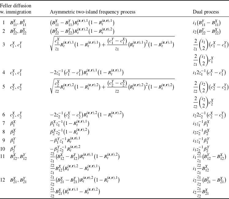
, by means of the culling procedure. Each of the parameters can be traced to those of the associated two-dimensional Feller diffusions with immigration, and we explain the relation between the parameters in Table 1. If the parameters
 $B^X_{ij}$
,
 $B^Y_{ij}$
with
 $i\not=j$
, and the variances
 $c^X_i,c^Y_i$
are non-zero for
 $i,j=1,2$
, we obtain a structured version of the Gillespie–Wright–Fisher diffusion introduced in [Reference Gillespie14,Reference Gillespie15]. If
 $c_i^X=c_i^Y$
for
 $i=1,2$
, we recover the two-island diffusion. Furthermore, if
 $c_1^X=c_1^Y$
and
 $c_2^X=c_2^Y=0$
, the process specializes to the seed bank diffusion.
Relation between the parameters of the Feller diffusions with immigration and those of their associated asymmetric two-island frequency process, as well as those of its moment dual.

The main steps to prove that
 $\textbf{R}^{(\textbf{z},\textbf{r})}$
arises from the relative frequency associated with two independent two-dimensional Feller diffusions with immigration as a limit when the sampling times become dense in the culling procedure are: first, we describe the dynamics of the relative frequency process of type-
 $\textbf{x}$
individuals (when the total size of each island is allowed to vary in time) as the solution to a martingale problem; we next show that the SDE associated with the process
 $\textbf{R}^{(\textbf{z},\textbf{r})}$
has a unique strong solution, which is a Feller process. The previous steps allow us to reduce the convergence of the culling procedure to a mere convergence of infinitesimal generators, which is the third step.
1.3. Moment duality for the asymmetric two-island frequency process
In Section 4 we show, under some conditions on the parameters of
 $\textbf{R}^{(\textbf{z},\textbf{r})}$
, that there exists a two-dimensional continuous-time Markov chain
 $\textbf{N}^{(\textbf{z},\textbf{n})}\;:\!=\;\big\{\textbf{N}^{(\textbf{z},\textbf{n})}_t=\big(N^{(\textbf{z},\textbf{n}),1}_t,N^{(\textbf{z},\textbf{n}),2}_t\big)\colon t\geq0\big\}$
such that, for every
 $t>0$
and for every initial condition in their respective state spaces
 $\textbf{n}=(n_1,n_2)$
and
 $\textbf{r}=(r_1,r_2)$
, the following relation holds:
 $$\mathbb{E}\Big[r_1^{\textbf{N}_t^{(\textbf{z},\textbf{n}),1}}r_2^{\textbf{N}_t^{(\textbf{z},\textbf{n}),2}} \mid\textbf{N}^{(\textbf{z},\textbf{n})}_0 = (n_1,n_2)\Big] =\mathbb{E}\big[(\textbf{R}^{(\textbf{z},\textbf{r}),1})^{n_1}(\textbf{R}^{(\textbf{z},\textbf{r}),2})^{n_2} \mid\textbf{R}^{(\textbf{z},\textbf{r})}_0=(r_1,r_2)\big].$$
We introduce a cemetery state
 $\Delta$
and we assume that
 $\textbf{r}^{\Delta}=0$
for all
 $\textbf{r}\in[0,1]^2$
. For each
 $(i_1,i_2),(j_1,j_2)\in\mathbb{N}_0^2\cup\{\Delta\}$
and
 $\textbf{z}=(z_1,z_2)\in(0,\infty)^2$
we define the following set of real numbers, which should be thought of as transition rates:
 \begin{equation*} q_{(i_1,i_2),(j_1,j_2)}^{\textbf{z}} = \begin{cases} i_1\dfrac{\beta_1^Y}{z_1} + i_2\dfrac{\beta_2^Y}{z_2} & \mbox{if }(j_1,j_2)=\Delta, \\[3mm] \displaystyle i_1s_1 + i_2\frac{z_1}{z_2}\big(B_{21}^Y-B_{21}^X\big) + \frac{2}{z_1}\binom{i_1}{2}\big(c_1^X-c_1^Y\big) & \mbox{if }(j_1,j_2)=(i_1+1,i_2), \\[3mm] \displaystyle i_2s_2 + i_1\frac{z_2}{z_1}\big(B_{12}^Y-B_{12}^X\big) + \frac{2}{z_2}\binom{i_2}{2}\big(c_2^X-c_2^Y\big) & \mbox{if }(j_1,j_2)=(i_1,i_2+1), \\[3mm] i_1B_{12}^X\dfrac{z_2}{z_1} & \mbox{if }(j_1,j_2)=(i_1-1,i_2+1), \\[3mm] i_2B_{21}^X\dfrac{z_1}{z_2} & \mbox{if }(j_1,j_2)=(i_1+1,i_2-1), \\[3mm] \displaystyle i_1\frac{\beta_1^X}{z_1} + \frac{2}{z_1}\binom{i_1}{2}c_1^X & \mbox{if }(j_1,j_2)=(i_1-1,i_2), \\[3mm] \displaystyle i_2\frac{\beta_2^X}{z_2} + \frac{2}{z_2}\binom{i_2}{2}c_2^X & \mbox{if }(j_1,j_2)=(i_1,i_2-1), \end{cases}\end{equation*}
where
 $s_i=\big(B_{ii}^Y-B_{ii}^X\big) + ({2}/{z_i})\big(c_i^X-c_i^Y\big)$
for
 $i=1,2$
.
If
 $q^{\textbf{z}}_{(i_1,i_2),(j_1,j_2)}\geq0$
for all
 $(i_1,i_2),(j_1,j_2)\in\mathbb{N}^2_0\cup\{\Delta\}$
, the continuous-time Markov chain
 $\textbf{N}^{(\textbf{z},\textbf{n})}$
has state space
 $\mathbb{N}_0^2\cup\{\Delta\}$
such that
 $\textbf{N}^{(\textbf{z},\textbf{n})}_0=\textbf{n}$
with
 $\textbf{n}=(n_1,n_2)\in\mathbb{N}^2_0$
, and generator given by
 $\mathcal{Q}^{\textbf{z}}=\big\{q^{\textbf{z}}_{(i_1,i_2),(j_1,j_2)}\colon(i_1,i_2),(j_1,j_2)\in\mathbb{N}_0^2\cup\{\Delta\}\big\}$
.
This relation between the moments of
 $\textbf{R}^{(\textbf{z},\textbf{r})}$
and the probability-generating function of
 $\textbf{N}^{(\textbf{z},\textbf{n})}$
is known as moment duality and constitutes a fundamental tool in population genetics. The most important example of this relation is the duality between Wright–Fisher diffusion and the Kingman coalescent. Moment duality formally links the evolution of a population with its ancestry. There are several other examples, for instance the celebrated ancestral selection graph [Reference Krone and Neuhauser23, Reference Neuhauser and Krone25] gives a notion of extended ancestry for Wright–Fisher diffusion with selection via moment duality. Additionally, duality has been used for the two-island model and the seed bank model in the presence of mutation in [Reference Blath, Buzzoni, González Casanova and Wilke-Berenguer4]. In [Reference González Casanova, Pardo and Pérez18], the duality between Gillespie–Wright–Fisher diffusion and a coalescing/pairwise-branching process was established and interpreted in terms of efficiency in [Reference González Casanova, Miró-Pina and Pardo17].
The existence of a moment dual for the asymmetric two-island frequency process generalizes all the results in the previous paragraph. An interesting fact about this new duality result is that in the dual process the particles can produce offsprings of both types.
Table 1 presents a dictionary that translates the different parameters of the Feller diffusions with immigration into the parameters of the asymmetric two-island frequency processes and the parameters of their duals. This is useful to understand how the three families of processes are related. For the last column, we remark that the parameters of the moment dual of the asymmetric two-island frequency process must fulfill some conditions to ensure the existence of the process (see Theorem 4.1).
In the first two rows of Table 1, we see that the differences between the Malthusians associated with the Feller diffusions with immigration
 $\big(B_{ii}^X-B_{ii}^Y,\ i=1,2\big)$
, become the coefficients of logistic drift terms in the asymmetric two-island frequency process associated with selection, and in the moment dual they become branching rates.
In rows 3–6 of Table 1, we can observe that the variances of each of the Feller diffusions have three different roles in the associated frequency process. The variances of the process
 $\textbf{X}$
 $\big(c_i^X$
,
 $i=1,2\big)$
dictate the strength of the random genetic drift for each island. The differences of the variances
 $\big(c_i^Y-c_i^X,\ i=1,2\big)$
, which are assumed to satisfy the condition
 $c_i^Y-c_i^X\leq 0$
for
 $i=1,2$
in order for the moment dual to exist, represent a frequency-dependent random genetic drift factor, and they also contribute with extra logistic drift terms in the asymmetric two-island frequency process. As expected, the random genetic drift is dual to Kingman’s coalescence. Furthermore, for the dual process the differences
 $c_i^X-c_i^Y$
,
 $i=1,2$
, determine the rate of pairwise branching and give an extra (individual) branching rate.
In rows 7–10 we consider the immigration terms of the Feller diffusion. These become drift terms that take each of the components of the asymmetric two-island frequency process away from its boundary points
 $\{0,1\}$
. In the dual, they become death rates (the rate at which an individual is removed) and killing rates (the rate at which the process is absorbed in a cemetery state).
Finally, in the last two rows we have the parameters that govern the cross-production of individuals, i.e. the way individuals on island 1 produce individuals on island 2, and vice versa. In the frequency process, the term
 $({z_2}/{z_1})B_{12}^X$
represents a drift towards identity, while the term
 $({z_2}/{z_1})\big(B_{12}^X -B_{12}^Y\big)$
introduces a novel drift term that resembles selection but depends on the frequencies in both islands rather than just one. In the moment dual, the term
 $({z_2}/{z_1})B_{12}^X$
corresponds to the migration rate (i.e. the rate at which individuals move from island 1 to island 2), while
 $({z_2}/{z_1})\big(B_{12}^Y-B_{12}^X\big)$
represents a branching/migration term that determines the rate at which individuals on island 1 reproduce, with the newborn individuals allocated to island 2. The roles of
 $B_{21}^X$
and
 $B_{21}^Y$
are similar.
1.4. The large-population deterministic limit
To understand the expected long-time behavior of the the asymmetric two-island frequency process, in Section 5 we send the total mass of the population on each island, fixed at each of the sampling times, to infinity and obtain a system of ordinary differential equations (ODEs). The resulting ODE is given by
 \begin{equation} \begin{aligned} \frac{{\mathrm{d}}}{{\mathrm{d}} t}r^{1}_t & = B^X_{12}\big(r^{2}_t-r^{1}_t\big) - \big(B^X_{12}-B^Y_{12}\big)\big(r^{1}_tr^{2}_t-r^{1}_t\big) + \big(B_{11}^X-B_{11}^Y\big)r^{1}_t\big(1-r^{1}_t\big), \\[4pt] \frac{{\mathrm{d}}}{{\mathrm{d}} t}r^{2}_t & = B^X_{21}\big(r^{1}_t-r^{2}_t\big) - \big(B^X_{21}-B^Y_{21}\big)\big(r^{1}_tr^{2}_t-r^{2}_t\big) + \big(B_{22}^X-B_{22}^Y\big)r^{2}_t\big(1-r^{2}_t\big), \quad t\geq0. \end{aligned}\end{equation}
Note that a negative
 $B^X_{ij}$
is only possible if
 $i=j$
, and this corresponds to a tendency to produce fewer than one individual of type
 $\textbf{x}$
.
The first term on each line pushes the solutions towards the identity line. The other terms depend on the differences between the reproduction rates of each type. Each of them pushes the solution towards one of the boundary points
 $\{(0,0), (1,1)\}$
which are associated with the event of fixation of one of the types in the population. However, at each point of the unit square, all the forces act simultaneously and complex behavior arises. To predict which type of individuals will go to fixation we need to consider all of the parameters, and it is even possible that the system of ODEs points to an internal point, implying that this complex interaction can favor coexistence.
To visualize the complexity of the interaction between these parameters we invite the reader to visit the web page of Julio Nava (https://julionava.shinyapps.io/app_prueba/), where it is possible to find a user-friendly interface that solves the system of ODEs numerically and presents different plots of interest.
1.5. The benefits of sustaining a seed bank
Recall the interpretation of islands 1 and 2 as active and dormant. In this section we study a toy model that gives some insight on the advantage for populations sustaining seed banks. Here,
 $\textbf{x}$
sustains a seed bank, while
 $\textbf{y}$
does not. To be precise, in (1.3) we let
 $B_{12}^Y=B_{21}^Y=B_{22}^Y=0$
and
 $B_{22}^X=-B_{12}^X$
. Then, the system reduces to
 \begin{equation} \begin{aligned} \frac{{\mathrm{d}}}{{\mathrm{d}} t}r^{1}_t & = B^X_{12}r^{2}_t\big(1-r^{1}_t\big) + \big(B_{11}^X-B_{11}^Y\big)r^{1}_t\big(1-r^{1}_t\big), \\ \frac{{\mathrm{d}}}{{\mathrm{d}} t}r^{2}_t & = B^X_{21}r^{1}_t\big(1-r^{2}_t\big) - B^X_{12}r^{2}_t\big(1-r^{2}_t\big), \quad t\geq0. \end{aligned}\end{equation}
Observe that the solution to the second equation is given by
 \begin{equation*} r^{2}_t = 1 - \big(1-r^2_0\big)\exp\bigg\{{-}\int_0^t\big[B^X_{21}r^{1}_s-B^X_{12}r_s^2\big]\,{\mathrm{d}} s\bigg\}, \quad t\geq0.\end{equation*}
Now, as only type-
 $\textbf{x}$
individuals produce seeds, it is reasonable to assume that the frequency of
 $\textbf{x}$
-type seeds at time zero is unity, i.e.
 $r^2_0=1$
. Note that this implies that
 \begin{equation} r^2_t=1 \quad \text{for all $t\geq 0$}.\end{equation}
So, if
 $r_0^2=1$
, by substituting (1.5) in (1.4) we obtain
 \[ \frac{{\mathrm{d}}}{{\mathrm{d}} t}r^{1}_t = B^X_{12}\big(1-r^{1}_t\big) + \big(B_{11}^X-B_{11}^Y\big)r^{1}_t\big(1-r^{1}_t\big), \quad t>0,\]
which has a solution given by
 \begin{equation*} r^1_t = \frac{{\mathrm{e}}^{(A+B)t}-CA}{CB+{\mathrm{e}}^{(A+B)t}}, \quad t\geq0,\end{equation*}
with
 $A=B^X_{12}$
,
 $B=B_{11}^X-B_{11}^Y$
, and
 $C=({1-r_0^1})/({A+Br_0^1})$
.
It is now easy to see that if
 $B_{12}^X+B_{11}^X\geq B_{11}^Y$
, then type-
 $\textbf{x}$
individuals have a strong selective advantage, meaning that
 $\lim_{t\to\infty}r^1_t=1$
. On the other hand, if
 $B_{12}^X+B_{11}^X<B_{11}^Y$
, then
 \[ \lim_{t\to\infty}r^1_t=\frac{B^X_{12}}{B_{11}^Y-B_{11}^X}\in(0,1).\]
Note that
 $B_{12}^X+B_{11}^X$
is the rate at which type-
 $\textbf{x}$
individuals produce offspring and seeds of type
 $\textbf{x}$
. For this reason, we can say that if the population sustaining a seed bank reproduces faster, it will have a strong selective advantage, while if they are slower, the populations will coexist. In other words, we observe that the seed producers never have a strong selective disadvantage: coexistence is their worst-case scenario.
2. Relative frequency and total population size
As discussed in the previous section, we will distinguish between two different types
 $\textbf{x}$
and
 $\textbf{y}$
in the population distributed between two islands 1 and 2. The evolution of the total mass of individuals of types
 $\textbf{x}$
and
 $\textbf{y}$
on island i will be described by Feller diffusions with immigration
 $X^i$
and
 $Y^i$
respectively, for
 $i=1,2$
.
We will now characterize the relative frequency of individuals of type
 $\textbf{x}$
and the total size of the population associated with each of the different islands. To this end, for each island
 $i=1,2$
, let us consider the relative frequency process of individuals of type
 $\textbf{x}$
given by
 \begin{align} R^i_t \;:\!=\; \frac{X^i_t}{X^i_t+Y^i_t}1_{\{t\leq \tau^i\}} + R^i_{\tau^i} 1_{\{t>\tau^i\}}, \quad t\geq0, \qquad R_0^i=r^i,\end{align}
where
 $\tau^i=\inf\{t\geq0\colon X^{i}Y^{i}=0\}$
and
 $r^i=x^{i}/(x^{i}+y^{i})$
.
To obtain a complete description of the dynamics of the population we will also consider, for each
 $i=1,2$
, the total population size of island i defined by
 \begin{equation} Z^i_t \;:\!=\; X^i_t + Y^i_t, \quad t\geq0, \qquad Z^i_0=z^i,\end{equation}
where
 $z^i=x^i+y^i$
.
In the next result we obtain the dynamics of the process
 $(\textbf{R},\textbf{Z})\;:\!=\;(R^1,R^2,Z^1,Z^2)$
defined by (2.1) and (2.2). We note that
 $(\textbf{R},\textbf{Z})$
is a Markov process, and hence we will describe its evolution through the solution to a martingale problem in the next result. We denote the law of the process
 $(\textbf{R},\textbf{Z})$
starting from the initial position
 $(\textbf{r},\textbf{z})=(r^1,r^2,z^1,z^2)\in[0,1]^2\times(0,\infty)^2$
by
 $\mathbb{P}_{(\textbf{r},\textbf{z})}$
. Accordingly, we denote the associated expectation operator by
 $\mathbb{E}_{(r,z)}$
.
We denote by
 $\|\cdot\|$
the Euclidean norm on
 $\mathbb{R}^2$
, and for
 $\varepsilon\in(0,z^1\wedge z^2)$
and
 $L>\|\textbf{z}\|$
we denote by
 $\tau_{\varepsilon}\;:\!=\;\inf\{t>0\colon Z^1_t\wedge Z^2_t=\varepsilon\}$
and
 $\tau_L\;:\!=\;\inf\{t>0\colon Z^1_t\vee Z^2_t=L\}$
the first hitting times of level
 $\varepsilon$
(respectively L) for the process
 $Z^1\wedge Z^2$
(respectively
 $Z^1\vee Z^2$
). We remark that the process
 $(\textbf{R},\textbf{Z})$
stopped at the stopping time
 $\tau=\tau_{\varepsilon}\wedge\tau_L$
completely encodes the dynamics of the two subpopulations of types
 $\textbf{x}$
and
 $\textbf{y}$
on the different islands, originally described by the processes
 $\textbf{X}$
and
 $\textbf{Y}$
, before the size of the population on either island becomes relatively small or large.
The next result describes the dynamics of the process
 $(\textbf{R},\textbf{Z})$
until the stopping time
 $\tau$
. Its proof is just an application of Itô’s formula and we defer it to Appendix A.
Lemma 2.1. For any
 $f\in\mathcal{C}^2([0,1]^2\times\mathbb{R}_+^2)$
, the process
 \begin{equation*} f\big(R^1_{t\wedge\tau},R^2_{t\wedge\tau},Z^1_{t\wedge\tau},Z^2_{t\wedge\tau}\big) - f(r^1,r^2,z^1,z^2) - \int_0^{t\wedge\tau}\mathcal{L}f\big(R^1_s,R^2_s,Z^1_s,Z^2_s\big)\,{\mathrm{d}} s,\quad t\geq 0, \end{equation*}
is a local martingale where
 $\mathcal{L}f(r_1,r_2,z_1,z_2)=\sum_{i=1}^3B^i(r_1,r_2,z_1,z_2)$
and
 $B^i$
is given in (A.3)–(A.5) for
 $i=1,\ldots,3$
.
3. Asymmetric two-island frequency process and culling of general two-island models
In the previous section, we described the dynamics of the process
 $(\textbf{R},\textbf{Z})=(R^1,R^2,Z^1,Z^2)$
, stopped at the stopping time
 $\tau$
, as the solution to a martingale problem. In this section, we will construct the asymmetric frequency process
 $\textbf{R}^{(\textbf{z},\textbf{r})}$
, introduced in Section 1.2, from the process
 $(R^1,R^2,Z^1,Z^2)$
by a sampling/culling procedure similar to the one introduced in [Reference Caballero, González Casanova and Pérez8].
We start this section by showing that the process
 $\textbf{R}^{(z,r)}$
is well-defined as the unique strong solution to (1.2); the proof of this result is deferred to Appendix B.
Proposition 3.1. There exists a unique strong solution
 $\textbf{R}^{(\textbf{z},\textbf{r})}$
to (1.2) such that
 $\textbf{R}^{(\textbf{z},\textbf{r})}\in[0,1]^2$
for all
 $t\geq0$
 $\mathbb{P}$
-almost surely (a.s.). Furthermore, for any
 $t>0$
there exists
 $C(t)>0$
such that
 \begin{equation} \mathbb{E}\big[\big\|\textbf{R}^{(\textbf{z},\textbf{r})}_t-\textbf{R}^{(\textbf{z},\overline{\textbf{r}})}_t\big\|\big] \leq C(t)\|\textbf{r}-\overline{\textbf{r}}\|,\quad \textbf{r},\overline{\textbf{r}}\in[0,1]^2. \end{equation}
Remark 3.1. We note that in the particular case in which the Feller diffusions with immigration
 $\textbf{X}$
and
 $\textbf{Y}$
have the same distribution then, for
 $t>0$
, the SDE given in (1.2) takes the form
 \begin{align*} {\mathrm{d}} R^{(z,r),1}_t & = \bigg[B_{12}^X\frac{z_2}{z_1}\Big(R^{(z,r),2}_t-R^{(z,r),1}_t\Big) + \frac{\beta_1^X}{z_1}\Big(1-R^{(z,r),1}_t\Big) - \frac{\beta_1^X}{z_1}R^{(z,r),1}_t\bigg]\,{\mathrm{d}} t \\ & \quad + \sqrt{\frac{c_1^X}{z_1}R^{(z,r),1}_t\Big(1-R^{(z,r),1}_t\Big)}\,{\mathrm{d}} W^1_t, \\ {\mathrm{d}} R^{(z,r),2}_t & = \bigg[B_{21}^X\frac{z_1}{z_2}\Big(R^{(z,r),1}_t-R^{(z,r),2}_t\Big) + \frac{\beta_2^X}{z_2}\Big(1-R^{(z,r),2}_t\Big) - \frac{\beta_2^X}{z_2}R^{(z,r),2}_t\bigg]\,{\mathrm{d}} t \\ & \quad + \sqrt{\frac{c_2^X}{z_2}R^{(z,r),2}_t\Big(1-R^{(z,r),2}_t\Big)}\,{\mathrm{d}} W^2_t, \end{align*}
with
 $\textbf{R}^{(z,r)}_0=(r_1,r_2)$
. Hence, we recover the general two-island model as in [Reference Blath, Buzzoni, González Casanova and Wilke-Berenguer4, Remark 1.2].
In the next result we show that the process
 $\textbf{R}^{(\textbf{z},\textbf{r})}$
is Feller and we characterize the process by computing its infinitesimal generator; we defer the proof to Appendix C.
Proposition 3.2 For any
 $\textbf{z}=(z_1,z_2)\in(0,\infty)^2$
,
 $\textbf{R}^{(\textbf{z},\textbf{r})}$
is a Feller process and its infinitesimal generator is given, for any
 $f\in\mathcal{C}^2([0,1]^2)$
, by
 \begin{equation} \mathcal{L}^{\textbf{z}}f(r_1,r_2) \;:\!=\; \sum_{i=1}^2D^{i}_f(r_1,r_2,z_1,z_2) \quad \textit{for}\;\text{$\textbf{r}=(r_1,r_2)\in[0,1]^2$}, \end{equation}
where
 \begin{align*} & D^1_f(r_1,r_2,z_1,z_2) \;:\!=\; \\ & \partial_1f(\textbf{r})(1-r_1)\bigg(B_{11}^Xr_1+B^X_{12}\frac{z_2}{z_1}r_2+\frac{\beta_1^X}{z_1}\bigg) - \partial_1f(\textbf{r})r_1\bigg(B_{11}^Y(1-r_1)+B^Y_{12}\frac{z_2}{z_1}(1-r_2)+\frac{\beta_1^Y}{z_1}\bigg) \\ & + \partial_2f(\textbf{r})(1-r_2)\bigg(B_{21}^X\frac{z_1}{z_2}r_1+B^X_{22}r_2+\frac{\beta_2^X}{z_2}\bigg) - \partial_2f(\textbf{r})r_2\bigg(B_{21}^Y\frac{z_1}{z_2}(1-r_1)+B^Y_{22}(1-r_2)+\frac{\beta_2^Y}{z_2}\bigg), \\ & D^2_f(r_1,r_2,z_1,z_2) \;:\!=\; \\ & \frac{c_1^X}{z_1}(r_1(1-r_1)^2\partial^2_{11}f(\textbf{r})-2r_1(1-r_1)\partial_1f(\textbf{r})) + \frac{c_2^X}{z_2}(r_2(1-r_2)^2\partial^2_{22}f(\textbf{r})-2r_2(1-r_2)\partial_2f(\textbf{r})) \\ & + \frac{c_1^Y}{z_1}\big(r_1^2(1-r_1)\partial^2_{11}f(\textbf{r})+2r_1(1-r_1)\partial_1f(\textbf{r})\big) + \frac{c_2^Y}{z_2}\big(r_2^2(1-r_2)\partial^2_{22}f(\textbf{r})+2r_2(1-r_2)\partial_2f(\textbf{r})\big). \end{align*}
3.1. Culling of the population process
In Section 2 we obtained the evolution of the process
 $(\textbf{R},\textbf{Z})=(R^1,R^2,Z^1,Z^2)$
as the solution to a martingale problem. We recall that for each
 $i=1,2$
, the component
 $R^i$
represents the frequency of individuals of type
 $\textbf{x}$
on the ith island, while
 $Z^i$
describes its total population size.
As in many population models, we are interested in maintaining the total size of the population constant while allowing the frequency processes of individuals of type
 $\textbf{x}$
associated with each island,
 $(R^1,R^2)$
, to evolve randomly, obtaining a two-dimensional stochastic process. Inspired by [Reference Gillespie14] (see also [Reference Caballero, González Casanova and Pérez8, Section 4.2]) we will use a sampling method called culling, in which at each sampling time we take the total size of the population on each island back to a constant level. This method allows us to obtain a random description of the frequency processes under the assumption that the total size of the population on each island is constant.
Let us consider fixed population sizes
 $z_1,z_2>0$
for the first and second islands, respectively. For
 $\textbf{z}=(z_1,z_2)$
, consider a sequence of pseudo-Poisson processes
 $\big\{\overline{\textbf{R}}^{(\textbf{z},n)}_t=\big(\overline{R}^{(\textbf{z},n),1}_t,\overline{R}^{(\textbf{z},n),2}_t\big)\colon t\geq0\big\}_{n\geq 1}$
(see [Reference Kallenberg22, Chapter 10] for a detailed introduction to pseudo-Poisson processes). We denote the law of the process
 $\overline{\textbf{R}}^{(\textbf{z},n)}$
by
 $\textbf{P}_{\textbf{r}}$
when started at the state
 $\textbf{r}=(r_1,r_2)\in[0,1]^2$
. For each fixed
 $n\geq1$
, the Markov process
 $\overline{\textbf{R}}^{(\textbf{z},n)}$
has jump times
 $(T^{m,n})_{m\geq1}$
given by independent exponential random variables with rate n, and transition kernel
 $\{\kappa^{(z,n)}\colon n\geq 1\}$
defined for
 $\textbf{y}\in[0,1]^2$
and
 $A\in\mathcal{B}([0,1]^2)$
by
 \begin{align} \kappa^{(z,n)}(\textbf{y},A) & = \textbf{P}_{\textbf{y}}\big(\overline{R}^{(z,n)}_{T^{1,n}}\in A\big) \nonumber \\ & = \mathbb{P}_{(y_1,y_2,z_1,z_2)}\big(\big(R^{1}_{({1}/{n})\wedge\tau},R^{2}_{({1}/{n})\wedge\tau},Z^{1}_{({1}/{n})\wedge\tau}, Z^{2}_{({1}/{n})\wedge\tau}\big)\in A\times\mathbb{R}_+^2\big), \end{align}
where
 $\tau=\tau_{\varepsilon}\wedge\tau_L$
is defined in Section 2.
By the proof of [Reference Kallenberg22, Theorem 17.28], the process
 $\overline{\textbf{R}}^{(\textbf{z},n)}$
is Feller and has an infinitesimal generator given for any
 $f\in\mathcal{C}([0,1]^2)$
by
 \begin{equation} \overline{\mathcal{L}}^{(\textbf{z},n)}f(\textbf{r}) = n\int_{[0,1]^2}(f(\textbf{u})-f(\textbf{r}))\kappa^{(z,n)}(\textbf{r},\textrm{d}\textbf{u}), \quad \textbf{r}\in[0,1]^2.\end{equation}
For each
 $n\geq 1$
, we can think of
 $\overline{\textbf{R}}^{(\textbf{z},n)}_{T^{1,n}}$
as a sampling of the first two coordinates of the process
 $\big(R^1_{t\wedge\tau},R^2_{t\wedge\tau},Z^1_{t\wedge\tau},Z^2_{t\wedge\tau}\big)_{t\geq0}$
started at the position
 $(\textbf{r},\textbf{z})\in[0,1]^2\times\mathbb{R}_+^2$
at time
 $t={1}/{n}$
. Then, in order to define
 $\overline{\textbf{R}}^{(\textbf{z},n)}_{T^{2,n}}$
, we use the fact that the process
 $(R^1,R^2,Z^1,Z^2)$
is a homogeneous Markov process to restart the process
 $\big(R^1_{t\wedge\tau},R^2_{t\wedge\tau},Z^1_{t\wedge\tau},Z^2_{t\wedge\tau}\big)_{t\geq0}$
at the initial position
 $\big(R^1_{({1}/{n})\wedge \tau},R^2_{({1}/{n})\wedge \tau},z_1,z_2\big)$
and sample the process at time
 $t={1}/{n}$
. By proceeding with this algorithm we can define the process
 $\overline{\textbf{R}}^{(\textbf{z},n)}_t$
for any
 $t>0$
.
With this construction the process
 $\overline{\textbf{R}}^{(\textbf{z},n)}$
evolves in the time interval
 $[T^{m,n},T^{m+1,n})$
as the first two coordinates of the process
 $(R^1,R^2,Z^1,Z^2)$
on the interval
 $[0,({1}/{n})\wedge\tau)$
, starting from the initial position
 $\big(\overline{\textbf{R}}^{(\textbf{z},n),1}_{T^{m,n}},\overline{\textbf{R}}^{(\textbf{z},n),2}_{T^{m,n}},z_1,z_2\big)$
. Therefore, the process
 $\overline{\textbf{R}}^{(\textbf{z},n)}$
behaves like the first two coordinates of the process
 $(R^1,R^2,Z^1,Z^2)$
but with the fluctuations of the total size of the population at each island
 $(Z^1,Z^2)$
around
 $(z_1,z_2)$
becoming smaller as
 $n\to\infty$
, i.e. as the sampling times converge to zero.
We denote by
 $\mathbb{D}([0,T],[0,1]^2)$
the space of functions with càdlàg paths on [0, T] taking values on
 $[0,1]^2$
endowed with the Skorokhod topology. In the next result we show that the sequence of processes
 $\big\{\big(\overline{\textbf{R}}^{(\textbf{z},n)}\big)_{t\geq0}\colon n\geq 1\big\}$
converges weakly in the space
 $\mathbb{D}([0,T],[0,1]^2)$
for any
 $T>0$
to the process
 $\textbf{R}^{(\textbf{z},\textbf{r})}$
, which is the unique solution to the stochastic differential equation given in (1.2). By this convergence and the previous construction we can understand the process
 $\textbf{R}^{(\textbf{z},\textbf{r})}$
as describing the evolution of the frequency of individuals of type
 $\textbf{x}$
on each island but under the assumption that the total size of the population on the ith island is constant and given by
 $z_i>0$
for each
 $i=1,2$
.
Theorem 3.1. Assume that
 $\overline{\textbf{R}}^{(\textbf{z},n)}$
is started from
 $\textbf{r}\in[0,1]^2$
for every
 $n\geq1$
. Then, for any fixed
 $\textbf{z}=(z_1,z_2)\in(0,\infty)^2$
and
 $T>0$
,
 $\overline{\textbf{R}}^{(\textbf{z},n)}\to \textbf{R}^{(\textbf{z},\textbf{r})}$
as
 $n\to\infty$
weakly in
 $\mathbb{D}([0,T],[0,1]^2)$
.
Proof. We note that for each
 $n\geq 1$
, the process
 $\overline{\textbf{R}}^{(\textbf{z},n)}$
takes values in the set
 $[0,1]^2$
, which is compact, and the same holds true for the process
 $\textbf{R}^{(\textbf{z},\textbf{r})}$
. By Proposition 3.2,
 $\mathcal{C}^2([0,1]^2)$
contains the core of the generator
 $\mathcal{L}^{\textbf{z}}$
, and following [Reference Kallenberg22, Theorem 17.28], we only need to verify that, for any
 $f\in\mathcal{C}^2([0,1]^2)$
,
 $\overline{\mathcal{L}}^{(\textbf{z},n)}f\to \mathcal{L}^{\textbf{z}}f$
strongly as
 $n\to\infty$
. Applying (3.3) and (3.4), we can write, for each
 $n\geq 1$
,
 \begin{equation*} \overline{\mathcal{L}}^{(\textbf{z},n)}f(\textbf{r}) = n\big[\mathbb{E}_{(\textbf{r},\textbf{z})}[f(\textbf{R}_{({1}/{n})\wedge \tau})]-f(\textbf{r})\big], \quad \textbf{r}\in[0,1]^2. \end{equation*}
On the other hand, by noting that the function f only depends on the first two coordinates
 $(x_1,x_2)$
of any point
 $(x_1,x_2,z_1,z_2)\in[0,1]^2\times(0,\infty)^2$
we have, by Lemma 2.1,
 \begin{equation} f(\textbf{R}_{n^{-1}\wedge \tau}) = f(\textbf{r}) + \int_{0}^{n^{-1}\wedge \tau}\sum_{i=1}^2D^i_f\big(R^1_s,R^2_s,Z^1_s,Z^2_s\big)\,{\mathrm{d}} s + M_{n^{-1}\wedge\tau}, \end{equation}
where, for
 $i=1,2$
,
 $D^i_f$
is defined in Proposition 3.2 and M is a local martingale.
Let us define
 $B(\varepsilon,L)\;:\!=\;\{(x_1,x_2)\in\mathbb{R}_+^2\colon\varepsilon\leq x_i\leq L,\ i=1,2\}$
. Then, using the fact that
 $f\in\mathcal{C}^2([0,1]^2)$
and that
 $\big(R^1_t,R^2_t,Z^1_t,Z^2_t\big)\in[0,1]^2\times B(\varepsilon,L)$
for
 $t\in[0,\tau]$
, we can find a constant
 $C>0$
such that
 \begin{equation} \Bigg|\sum_{i=1}^2D^i_f\big(R^1_t,R^2_t,Z^1_t,Z^2_t\big)\Bigg| \leq C \quad \text{for $t\in[0,\tau]$, $\mathbb{P}$-a.s.} \end{equation}
Hence, taking expectations in (3.5) we have
 \begin{align} \overline{\mathcal{L}}^{(\textbf{z},n)}f(\textbf{r}) & = n\big[\mathbb{E}_{(\textbf{r},\textbf{z})}[f(\textbf{R}_{({1}/{n})\wedge \tau})] - f(\textbf{r})\big] \nonumber \\ & = n\mathbb{E}_{(\textbf{r},\textbf{z})}\Bigg[ \int_{0}^{n^{-1}\wedge\tau}\sum_{1=1}^2D^i_f\big(R^1_s,R^2_s,Z^1_s,Z^2_s\big)\,{\mathrm{d}} s\Bigg]. \end{align}
Now, by (3.6),
 $\big|n\int_{0}^{n^{-1}\wedge\tau}\sum_{1=1}^2D^i_f\big(R^1_s,R^2_s,Z^1_s,Z^2_s\big)\,{\mathrm{d}} s\big| \leq C$
 $\mathbb{P}$
-a.s., so (3.7) and dominated convergence give, for
 $\textbf{r}=(r_1,r_2)\in[0,1]^2$
,
 \begin{align*} \lim_{n\to\infty}\overline{\mathcal{L}}^{(\textbf{z},n)}f(\textbf{r}) & = \lim_{n\to\infty}n\mathbb{E}_{(\textbf{r},\textbf{z})}\Bigg[ \int_{0}^{n^{-1}\wedge \tau}\sum_{1=1}^2D^i_f\big(R^1_s,R^2_s,Z^1_s,Z^2_s\big)\,{\mathrm{d}} s\Bigg] \\ & = \sum_{1=1}^2D^i_f(r_1,r_2,z_1,z_2) = \mathcal{L}^{\textbf{z}}f(\textbf{r}). \end{align*}
To finish the proof we only need to show that the convergence given in this last result holds in the strong sense; this is achieved by an application of [Reference Böttcher, Schilling and Wang7, Theorem 1.33].
4. Moment duality for asymmetric two-island frequency processes
Throughout this section we will prove that the moment dual of the asymmetric two-island frequency process
 $\textbf{R}^{(\textbf{z},\textbf{r})}$
, introduced in Section 1.2 is given by the continuous-time Markov chain
 $\textbf{N}^{(\textbf{z},\textbf{n})}$
given in Section 1.3. To obtain this result we will rely on martingale techniques, which are quite useful for solving this type of problem. The following proposition is a direct consequence of [Reference Ethier and Kurtz11, Theorem 4.11], taking H bounded and continuous, and
 $\alpha=\beta=0$
, and can also be seen as a small modification of [Reference Jansen and Kurt21, Proposition 1.2].
Proposition 4.1. Let
 $Y^{(1)}=\big\{Y^{(1)}_t\colon t\geq 0\big\}$
and
 $Y^{(2)}=\big\{Y^{(2)}_t\colon t\geq 0\big\}$
be two Markov processes taking values on
 $E_1$
and
 $E_2$
, respectively. Let
 $H\colon E_1\times E_2\rightarrow \mathbb{R}$
be a bounded and continuous function, and assume that there exists a Borel-measurable function
 $g\colon E_1\times E_2\mapsto \mathbb{R}$
such that, for every
 $n\in E_1$
,
 $x\in E_2$
, and every
 $T>0$
, the processes
 $M^{(1)}=\big\{M_t^{(1)}\colon0\le t\le T\big\}$
and
 $M^{(2)}=\big\{M_t^{(2)}, 0\le t\le T\big\}$
, defined as
 \begin{equation*} M_t^{(1)} \;:\!=\; H\big(Y^{(1)}_t,x\big) - \int_0^t g\big(Y^{(1)}_s,x\big)\,\mathrm{d}s, \qquad M_t^{(2)} \;:\!=\; H\big(n,Y^{(2)}_t\big) - \int_0^t g\big(n, Y^{(2)}_s\big)\,\mathrm{d}s \end{equation*}
are martingales with respect to the natural filtration of
 $Y^{(1)}_t$
and
 $Y^{(2)}_t$
, respectively. Then the processes
 $Y^{(1)}$
and
 $Y^{(2)}$
are dual with respect to H.
The previous result defines a general duality relation between two Markov processes. Because we are interested in moment duality we will use Proposition 4.1 with the particular case of
 $H(x,y,n,m)=x^ny^m$
with
 $x,y\in[0,1]$
and
 $n,m\in\mathbb{N}_0$
. We assume that
 $H(x,y,n,m)=0$
for
 $(x,y)\in[0,1]^2$
and
 $(n,m)=\Delta$
.
Theorem 4.1. Assume that
 $q^{\textbf{z}}_{(i_1,i_2),(j_1,j_2)}\geq0$
for all
 $(i_1,i_2),(j_1,j_2)\in\mathbb{N}_0^2\cup\{\Delta\}$
. Then, for all
 $\textbf{r}=(r_1,r_2)\in[0,1]^2$
,
 $\textbf{n}=(n_1,n_2)\in\mathbb{N}_0^2\cup\{\Delta\}$
, and
 $t>0$
,
 \begin{equation*} \mathbb{E}\big[\big(R_t^{({\textbf{z}},{\textbf{r}}),1}\big)^{n_1}\big(R_t^{({\textbf{z}},{\textbf{r}}),2}\big)^{n_2}\big] = \mathbb{E}\Big[r_1^{N^{(\textbf{z},\textbf{n}),1}_t}r_2^{N^{(\textbf{z},\textbf{n}),2}_t}\Big]. \end{equation*}
Proof. We will consider
 $\mathbb{N}_0^2\cup \{\Delta\}$
endowed with the discrete topology and
 $[0,1]^2\times\mathbb{N}_0^2\cup \{\Delta\}$
with the product topology. We recall that, for every fixed
 $(r_1,r_2)\in[0,1]^2$
,
 $H(r_1,r_2,n_1,n_2)=r_1^{n_1}r_2^{n_2}$
with
 $H(r_1,r_2,n_1,0)=r_1^{n_1}$
,
 $H(r_1,r_2,0,n_2)=r_2^{n_2}$
,
 $H(r_1,r_2,0,0)=1$
, and
 $H(r_1,r_2,n_1,n_2)=0$
if
 $(n_1,n_2)=\Delta$
, which are bounded and continuous. In addition, for every fixed
 $\textbf{n}=(n_1,n_2)\in \mathbb{N}_0^2\cup \{\Delta\}$
,
 $H(r_1,r_2,n_1,n_2)=r_1^{n_1}r_2^{n_2}1_{\{\textbf{n}\not=\Delta\}}$
is continuous. Therefore, we conclude that
 $H\colon\mathbb{N}_0^2\cup \{\Delta\}\times [0,1]^2\mapsto[0,1] $
is continuous.
We observe that
 $H(\cdot,n_1,n_2)$
is a polynomial in
 $[0,1]^2$
for fixed
 $(n_1,n_2)\in\mathbb{N}_0^2\cup\{\Delta\}$
. This fact clearly implies that
 $H(\cdot,n_1,n_2)\in\mathcal{C}^2([0,1]^2)$
, and hence it lies in the domain of the generator
 $\mathcal{L}^{\textbf{z}}$
. Therefore, the process
 $H\big(R_t^{({\textbf{z}},{\textbf{r}}),1},R_t^{({\textbf{z}},{\textbf{r}}),2},n_1,n_2\big) - \int_0^t\mathcal{L}^{\textbf{z}}H\big(R_s^{({\textbf{z}},{\textbf{r}}),1},R_s^{({\textbf{z}},{\textbf{r}}),2},n_1,n_2\big)\,{\mathrm{d}} s$
is a martingale.
Additionally, as in the proof of [Reference González Casanova, Pardo and Pérez18, Lemma 2], we have that for fixed
 $(r_1,r_2)\in[0,1]^2$
the function
 $H(r_1,r_2,\cdot)$
lies in the domain of the generator
 $\mathcal{Q}^{\textbf{z}}$
, which implies that the process
 \[ H\big(r_1,r_2,N^{(\textbf{z},\textbf{n}),1}_t,N^{(\textbf{z},\textbf{n}),2}_t\big) - \int_0^t\mathcal{Q}^{\textbf{z}}H\big(r_1,r_2,N^{(\textbf{z},\textbf{n}),1}_s,N^{(\textbf{z},\textbf{n}),2}_s\big)\,{\mathrm{d}} s \]
is also a martingale. In view of Proposition 4.1, we will compute
 $\mathcal{L}^{\textbf{z}}H(r_1,r_2,n_1,n_2)$
for
 $(r_1,r_2)\in[0,1]^2$
and
 $(n_1,n_2)\in\mathbb{N}_0^2\backslash\{(0,0)\}$
. Using Proposition 3.2, we obtain
 \begin{equation} \mathcal{L}^{\textbf{z}}H(r_1,r_2,n_1,n_2) = \sum_{i=1}^2D^i_H(r_1,r_2,z_1,z_2), \end{equation}
with
 \begin{align} D^1_H(r_1,r_2,z_1,z_2) & = n_1r^{n_1-1}_1r_2^{n_2}(1-r_1)\bigg(B_{11}^Xr_1+B^X_{12}\frac{z_2}{z_1}r_2+\frac{\beta_1^X}{z_1}\bigg) \notag \\ & \quad - n_1r_1^{n_1}r_2^{n_2}\bigg(B_{11}^Y(1-r_1)+B^Y_{12}\frac{z_2}{z_1}(1-r_2)+\frac{\beta_1^Y}{z_1}\bigg) \notag \\ & \quad + n_2r_1^{n_1}r_2^{n_2-1}(1-r_2)\bigg(B_{21}^X\frac{z_1}{z_2}r_1+B^X_{22}r_2+\frac{\beta_2^X}{z_2}\bigg) \notag \\ & \quad - n_2r_1^{n_1}r_2^{n_2}\bigg(B_{21}^Y\frac{z_1}{z_2}(1-r_1)+B^Y_{22}(1-r_2)+\frac{\beta_2^Y}{z_2}\bigg) \notag \\ & = \big(r_1^{n_1+1}r_2^{n_2}-r_1^{n_1}r_2^{n_2}\big)\bigg[n_1\big(B_{11}^Y-B_{11}^X\big) + n_2\frac{z_1}{z_2}\big(B_{21}^Y-B_{21}^X\big)\bigg] \notag \\ & \quad + \big(r_1^{n_1-1}r_2^{n_2}-r_1^{n_1}r_2^{n_2}\big)n_1\frac{\beta^X_1}{z_1} \notag \\ & \quad + \big(r_1^{n_1}r_2^{n_2+1}-r_1^{n_1}r_2^{n_2}\big)\bigg[n_2\big(B_{22}^Y-B_{22}^X\big) + n_1\frac{z_2}{z_1}\big(B_{12}^Y-B_{12}^X\big)\bigg] \notag \\ & \quad + \big(r_1^{n_1}r_2^{n_2-1}-r_1^{n_1}r_2^{n_2}\big)n_2\frac{\beta^X_2}{z_2} + \big(r_1^{n_1-1}r_2^{n_2+1}-r_1^{n_1}r_2^{n_2}\big)n_1B^X_{12}\frac{z_2}{z_1} \notag \\ & \quad + \big(r_1^{n_1+1}r_2^{n_2-1}-r_1^{n_1}r_2^{n_2}\big)n_2B^X_{21}\frac{z_1}{z_2} - r_1^{n_1}r_2^{n_2}\bigg[n_1\frac{\beta_1^Y}{z_1}+n_2\frac{\beta_2^Y}{z_2}\bigg], \end{align}
 \begin{align} D_H^2(r_1,r_2,z_1,z_2) & = \frac{c_1^X}{z_1}\big((1-r_1)^2{n_1}(n_1-1)r_1^{n_1-1}r_2^{n_2}-2(1-r_1)n_1r_1^{n_1}r_2^{n_2}\big) \notag \\ & \quad + \frac{c_2^X}{z_2}\big((1-r_2)^2n_2(n_2-1)r_1^{n_1}r_2^{n_2-1}-2(1-r_2)n_2r_1^{n_1}r_2^{n_2}\big) \notag \\ & \quad + \frac{c_1^Y}{z_1}\big((1-r_1)n_1(n_1-1)r_1^{n_1}r_2^{n_2}+2(1-r_1)n_1r_1^{n_1}r_2^{n_2}\big) \notag \\ & \quad + \frac{c_2^Y}{z_2}\big((1-r_2)n_2(n_2-1)r_1^{n_1}r_2^{n_2}+2(1-r_2)n_2r_1^{n_1}r_2^{n_2}\big) \notag \\ & = \big(r_1^{n_1+1}r_2^{n_2}-r_1^{n_1}r_2^{n_2}\big) \bigg(\frac{2n_1}{z_1}\big(c_1^X-c_1^Y\big) + \frac{n_1(n_1-1)}{z_1}\big(c_1^X-c_1^Y\big)\bigg) \notag \\ & \quad + \big(r_1^{n_1-1}r_2^{n_2}-r_1^{n_1}r_2^{n_2}\big)n_1(n_1-1)\frac{c_1^X}{z_1} \notag \\ & \quad + \big(r_1^{n_1}r_2^{n_2+1}-r_1^{n_1}r_2^{n_2}\big) \bigg(\frac{2n_2}{z_2}\big(c_2^X-c_2^Y\big)+\frac{n_2(n_2-1)}{z_2}\big(c_2^X-c_2^Y\big)\bigg) \notag \\ & \quad + \big(r_1^{n_1}r_2^{n_2-1}-r_1^{n_1}r_2^{n_2}\big)n_2(n_2-1)\frac{c_2^X}{z_2}. \end{align}
Therefore, applying (4.2) and (4.3) in (4.1), we obtain
 \begin{align*} \mathcal{L}^{\textbf{z}}H(r_1,r_2,n_1,n_2) & = \big(r_1^{n_1+1}r_2^{n_2}-r_1^{n_1}r_2^{n_2}\big)\bigg[n_1\big(B_{11}^Y-B_{11}^X\big) + n_2\frac{z_1}{z_2}\big(B_{21}^Y-B_{21}^X\big) \\ & \qquad\qquad\qquad\qquad\qquad + \frac{2n_1}{z_1}\big(c_1^X-c_1^Y\big) + \frac{n_1(n_1-1)}{z_1}\big(c_1^X-c_1^Y\big)\bigg] \\ & \quad + \big(r_1^{n_1}r_2^{n_2+1}-r_1^{n_1}r_2^{n_2}\big)\bigg[n_2\big(B_{22}^Y-B_{22}^X\big) + n_1\frac{z_2}{z_1}\big(B_{12}^Y-B_{12}^X\big) \\ & \qquad\qquad\qquad\qquad\qquad + \frac{2n_2}{z_2}\big(c_2^X-c_2^Y\big) + \frac{n_2(n_2-1)}{z_2}\big(c_2^X-c_2^Y\big)\bigg] \\ & \quad + \big(r_1^{n_1-1}r_2^{n_2}-r_1^{n_1}r_2^{n_2}\big) \bigg[n_1\frac{\beta^X_1}{z_1}+n_1(n_1-1)\frac{c_1^X}{z_1}\bigg] \\ & \quad + \big(r_1^{n_1}r_2^{n_2-1}-r_1^{n_1}r_2^{n_2}\big) \bigg[n_2\frac{\beta^X_2}{z_2}+n_2(n_2-1)\frac{c_2^X}{z_2}\bigg] \\ & \quad + \big(r_1^{n_1-1}r_2^{n_2+1}-r_1^{n_1}r_2^{n_2}\big)n_1B^X_{12}\frac{z_2}{z_1} + \big(r_1^{n_1+1}r_2^{n_2-1}-r_1^{n_1}r_2^{n_2}\big)n_2B^X_{21}\frac{z_1}{z_2} \\ & \quad - r_1^{n_1}r_2^{n_2}\bigg[n_1\frac{\beta_1^Y}{z_1}+n_2\frac{\beta_2^Y}{z_2}\bigg] = \mathcal{Q}^{\textbf{z}}H(r_1,r_2,n_1,n_2). \end{align*}
Meanwhile, for the case
 $(n_1,n_2)=(0,0)$
, we have that
 $\mathcal{L}^{\textbf{z}}H(r_1,r_2,0,0)=0=\mathcal{Q}^{\textbf{z}}H(r_1,r_2,0,0)$
for
 $(r_1,r_2)\in[0,1]^2$
. Similarly,
 $\mathcal{L}^{\textbf{z}}H(r_1,r_2,\Delta)=0=\mathcal{Q}^{\textbf{z}}H(r_1,r_2,\Delta)$
for
 $(r_1,r_2)\in[0,1]^2$
. Therefore, the result follows from Proposition 4.1.
5. Large-population asymptotics of asymmetric two-island frequency processes
To disentangle the effects and interactions of the different forms of selection included in our model, we will send the population size to infinity to isolate the deterministic action of selection from the random noise coming from the random genetic drift. To this end, in this section we obtain the deterministic limit obtained when the size of the population on each island grows to infinity. This will allow us to study in the next section the deterministic system that emerges.
5.1. Large-population limit of asymmetric two-island frequency processes
Throughout this section we will assume that the total sizes of the population of each of the islands, given by
 $z_1$
and
 $z_2$
, are equal to a constant
 $z>0$
. For this reason, we will use
 $\textbf{R}^{(z,\textbf{r})}=\big(R^{(z,\textbf{r}),1},R^{(z,\textbf{r}),2}\big)$
to denote the unique solution to (1.2), and study the asymptotic behavior of the process
 $\textbf{R}^{(z,\textbf{r})}$
as z increases to infinity. The limiting object, which we denote by
 $\textbf{R}^{(\infty,\textbf{r})}=\big(R^{(\infty,\textbf{r}),1},R^{(\infty,\textbf{r}),2}\big)$
, is deterministic and it is the unique solution to the ordinary differential equation
 \begin{equation} {\mathrm{d}} R^{(\infty,r),i}_t = \tilde{b}^i\big(\textbf{R}^{(\infty,\textbf{r})}_t\big)\,{\mathrm{d}} t, \quad t>0, \ i=1,2,\end{equation}
with
 $\textbf{R}^{(\infty,\textbf{r})}_0=(r_1,r_2)$
and where, for
 $\textbf{x}=(x_1,x_2)\in[0,1]^2$
,
 \begin{align} \tilde{b}^1(\textbf{x}) & = \big(B_{11}^X-B_{11}^Y\big)x_1(1-x_1) + B_{12}^X(1-x_1)x_2 - B_{12}^Yx_1(1-x_2), \\ \tilde{b}^2(\textbf{x}) & = \big(B_{22}^X-B_{22}^Y\big)x_2(1-x_2) + B_{21}^X(1-x_2)x_1 - B_{21}^Yx_2(1-x_1). \nonumber\end{align}
The next result shows the convergence of the process
 $\textbf{R}^{(z,\textbf{r})}$
to
 $\textbf{R}^{(\infty,\textbf{r})}$
in pth mean, uniformly on compact sets of
 $\mathbb{R}_+$
.
Theorem 5.1. For any
 $T>0$
and
 $p>1$
,
 $\lim_{z\to\infty}\mathbb{E}\big[\sup_{t\in[0,T]} \big\|\textbf{R}^{(z,\textbf{r})}_t-\textbf{R}^{(\infty,\textbf{r})}_t\big\|^p\big] = 0$
.
Proof. Using (1.2) together with (5.1), we obtain, for
 $i=1,2$
,
 \begin{align} R^{(z,\textbf{r}),i}_t-R^{(\infty,{\textbf{r}}),i}_t & = \int_0^t\big(\tilde{b}^i\big(\textbf{R}^{(z,\textbf{r})}_s\big) - \tilde{b}^i\big(\textbf{R}^{(\infty,\textbf{r})}_s\big) + a^i\big(\textbf{R}^{(z,\textbf{r})}_s\big)\big)\,{\mathrm{d}} s \notag \\ & \quad + \int_0^t\sqrt{\frac{c_i^X}{z}R^{({z},{\textbf{r}}),i}_s\big(1-R^{({z},{\textbf{r}}),i}_s\big)^2 + \frac{c_i^Y}{z}\big(R^{({z},{\textbf{r}}),i}_s\big)^2\big(1-R^{({z},{\textbf{r}}),i}_s\big)}\,{\mathrm{d}} W^{i}_s, \end{align}
where
 $\tilde{b}^i$
is given in (5.2) for
 $i=1,2$
, and
 \begin{equation*} a^i(\textbf{x}) = \frac{2}{z}\big(c_i^Y-c_i^X\big)x_i(1-x_i) + \frac{\beta_i^X}{z}(1-x_i) - \frac{\beta_i^Y}{z}x_i, \quad \textbf{x}\in[0,1]^2. \end{equation*}
A straightforward computation shows that, for
 $i=1,2$
, there exists a constant
 $C_i>0$
such that, for any
 $\textbf{x},\textbf{y}\in[0,1]^2$
,
 \begin{equation*} |\tilde{b}^i(\textbf{x})-\tilde{b}^i(\textbf{y})+a^{i}(\textbf{x})| \leq C_i(|x_1-y_1|+|x_2-y_2|) + \frac{2}{z}\big|c_i^Y-c_i^X\big| + \frac{\beta_i^X}{z} + \frac{\beta_i^Y}{z}. \end{equation*}
Hence, by Jensen’s inequality and the Burkholder–Davis–Gundy inequality, we obtain, for some constant
 $A_i>0$
and
 $i=1,2$
,
 \begin{align} & \mathbb{E}\big[\sup_{t\in[0,T]}\big|R^{({z},{\textbf{r}}),i}_t-R^{(\infty,{\textbf{r}}),i}_t\big|^p\big] \nonumber \\ & \leq 2^p\bigg[T^{p-1}\mathbb{E}\int_0^T\big|\tilde{b}^i\big(\textbf{R}^{(z,\textbf{r})}_s\big) - \tilde{b}^i\big(\textbf{R}^{(\infty,\textbf{r})}_s\big) + a^i\big(\textbf{R}^{(z,\textbf{r})}_s\big)\big|^p\,{\mathrm{d}} s \notag \\ & \qquad\quad + A_i\mathbb{E}\bigg[\int_0^T\bigg( \frac{c_i^X}{z}R^{({z},{\textbf{r}}),i}_s\big(1-R^{({z},{\textbf{r}}),i}_s\big)^2 + \frac{c_i^Y}{z}\big(R^{({z},{\textbf{r}}),i}_s\big)^2\big(1-R^{({z},{\textbf{r}}),i}_s\big)\bigg)\, {\mathrm{d}} s\bigg]^{p/2}\bigg] \notag \\ & \leq K_i\Bigg[T^{p-1}\mathbb{E}\int_0^T\sum_{i=1}^2 \big|R^{({z},{\textbf{r}}),i}_s-R^{(\infty,{\textbf{r}}),i}_s\big|^p\,{\mathrm{d}} s + \bigg(\frac{T}{z}\bigg)^{p}\big(2\big|c_i^Y-c_i^X\big| + \beta_i^X + \beta_i^Y\big)^p \nonumber \\ & \qquad\quad + \bigg(\frac{T}{z}\bigg)^{p/2}\big(c_i^Y+c_i^X\big)^{p/2}\Bigg] \notag \\ & \leq K_i\bigg[2T^{p-1}\mathbb{E}\int_0^T\sup_{u\in[0,s]} \big\|\textbf{R}^{(z,\textbf{r})}_u-\textbf{R}^{(\infty,\textbf{r})}_u\big\|^p\,{\mathrm{d}} s + \bigg(\frac{T}{z}\bigg)^{p}\big(2\big|c_i^Y-c_i^X\big| + \beta_i^X + \beta_i^Y\big)^p \nonumber \\ & \qquad\quad + \bigg(\frac{T}{z}\bigg)^{p/2}\big(c_i^Y+c_i^X\big)^{p/2}\bigg] \end{align}
for some constant
 $K_i>0$
, where in the last inequality we used the fact that
 $\big|R^{({z},{\textbf{r}}),i}_s-R^{(\infty,{\textbf{r}}),i}_s\big|^p \leq \big\|\textbf{R}^{(z,\textbf{r})}_s-\textbf{R}^{(\infty,\textbf{r})}_s\big\|^p$
for
 $s\in[0,T]$
and
 $i=1,2$
. Inequality (5.4) implies that, for
 $i=1,2$
, there exists a constant
 $\tilde{C}_i>0$
such that
 \begin{align*} \mathbb{E}\bigg[\sup_{t\in[0,T]}\big|R^{({z},{\textbf{r}}),i}_t-R^{(\infty,{\textbf{r}}),i}_t\big|^p\bigg] & \leq 2K_iT^{p-1}\int_0^T\mathbb{E}\bigg[\sup_{u\in[0,s]} \big\|\textbf{R}^{(z,\textbf{r})}_u-\textbf{R}^{(\infty,\textbf{r})}_u\big\|^p\bigg]\,{\mathrm{d}} s \\ & \quad + \tilde{C}_i(1+T^p)\bigg(\frac{1}{z^{p/2}}+\frac{1}{z^{p}}\bigg). \end{align*}
Therefore, by an application of Gronwall’s lemma we have
 \begin{equation*} \mathbb{E}\bigg[\sup_{t\in[0,T]}\big\|\textbf{R}^{(z,\textbf{r})}_t-\textbf{R}^{(\infty,\textbf{r})}_t\big\|^p\bigg] \leq 2^{p/2}(1+T^p)\sum_{i=1}^2\tilde{C}_i\bigg(\frac{1}{z^{p/2}}+\frac{1}{z^{p}}\bigg) \exp\Bigg\{2^{p/2+1}T^{p}\sum_{i=1}^2K_i\Bigg\}. \end{equation*}
Hence,
 \begin{multline} \lim_{z\to\infty}\mathbb{E}\bigg[ \sup_{t\in[0,T]}\big\|\textbf{R}^{(z,\textbf{r})}_t-\textbf{R}^{(\infty,\textbf{r})}_t\big\|^p\bigg] \\ \leq \lim_{z\to\infty}2^{p/2}(1+T^p)\sum_{i=1}^2\tilde{C}_i\bigg(\frac{1}{z^{p/2}}+\frac{1}{z^{p}}\bigg) \exp\Bigg\{2^{p/2+1}T^{p}\sum_{i=1}^2K_i\Bigg\} = 0, \end{multline}
which completes the proof.
5.2. Fluctuations of asymmetric two-island frequency processes
In this section we will study the fluctuations of the process
 $\textbf{R}^{(z,\textbf{r})}$
around its large-population limit
 $\textbf{R}^{(\infty,\textbf{r})}$
. To this end, let us define
 \begin{align} A^{(1)}_t & \;:\!=\; \big(B^X_{11}-B^Y_{11}\big)\big(2R_t^{(\infty,{\textbf{r}}),1}-1\big) + B_{12}^XR_t^{(\infty,{\textbf{r}}),2} - B_{12}^Y\big(R_t^{(\infty,{\textbf{r}}),2}-1\big), \\ A^{(2)}_t & \;:\!=\; \big(B^X_{22}-B^Y_{22}\big)\big(2R_t^{(\infty,{\textbf{r}}),2}-1\big) + B_{21}^XR_t^{(\infty,{\textbf{r}}),1} - B_{21}^Y\big(R_t^{(\infty,{\textbf{r}}),1}-1\big). \notag\end{align}
Let us introduce the process
 $\textbf{U}\;:\!=\;\big\{\textbf{U}_t=\big(U^1_t,U^2_t\big)\colon t\geq0\big\}$
where, for each
 $i=1,2$
and
 $t>0$
,
 \begin{equation*} U^{i}_t = \int_0^t\exp\bigg\{\int_0^sA^{(i)}_u\,{\mathrm{d}} u\bigg\} \sqrt{c_i^XR^{(\infty,{\textbf{r}}),i}_s\big(1-R^{(\infty,{\textbf{r}}),i}_s\big)^2 + c_i^Y\big(R^{(\infty,{\textbf{r}}),i}_s\big)^2\big(1-R^{(\infty,{\textbf{r}}),i}_s\big)}\,{\mathrm{d}} W^{i}_s.\end{equation*}
We note that the processes
 $U^1$
and
 $U^2$
are independent (by the independence of the Brownian motions
 $W^1$
and
 $W^2$
) and, for each
 $i=1,2,$
,
 $U^i$
is a zero-mean Gaussian process with covariance function
 $C_{U^i}$
given for
 $u,v\in\mathbb{R}_+$
by
 \begin{align*} C_{U^i}(u,v) &= \int_0^{u\wedge v}\exp\bigg\{2\int_0^sA^{(i)}_u\,{\mathrm{d}} u\bigg\}\big[c_i^XR^{(\infty,{\textbf{r}}),i}_s\big(1-R^{(\infty,{\textbf{r}}),i}_s\big)^2\\ &\qquad\qquad\qquad\qquad\qquad\qquad\!\! +c_i^Y\big(R^{(\infty,{\textbf{r}}),i}_s\big)^2\big(1-R^{(\infty,{\textbf{r}}),i}_s\big)\big]\,{\mathrm{d}} s.\end{align*}
Additionally, consider the process
 $\textbf{M}^{(z)}\;:\!=\;\big\{\textbf{M}^{(z)}=\big(M^{(z,1)}_t,M^{(z,2)}_t\big)\colon t\geq0\big\}$
defined for
 $t\geq0$
,
 $i=1,2$
as
 \begin{equation*} M^{(z,i)}_t \;:\!=\; \int_0^t\exp\bigg\{\int_0^sA^{(i)}_u\,{\mathrm{d}} u\bigg\} \sqrt{c_i^XR^{(z,{\textbf{r}}),i}_s\big(1-R^{(z,{\textbf{r}}),i}_s\big)^2 + c_i^Y\big(R^{(z,{\textbf{r}}),i}_s\big)^2\big(1-R^{(z,{\textbf{r}}),i}_s\big)}\,{\mathrm{d}} W^{i}_s.\end{equation*}
The proof of following auxiliary result is deferred to Appendix D.
Lemma 5.1 For any
 $T>0$
,
 $\lim_{z\to\infty}\mathbb{E}\big[\sup_{t\in[0,T]}\big\|\textbf{M}^{(z)}_t-\textbf{U}_t\big\|^2\big]=0$
.
In the next result we show that the sequence of processes
 $\{\sqrt{z}(\textbf{R}^{(z,\textbf{r})}-\textbf{R}^{(\infty,\textbf{r})})\colon z\geq 1\}$
is tight in the space
 $\mathbb{C}(\mathbb{R}_+,\mathbb{R}^2)$
, i.e. the space of continuous functions from
 $\mathbb{R}_+$
to
 $\mathbb{R}^2$
endowed with the topology of uniform convergence in compact sets.
Proposition 5.1 The family
 $\{\sqrt{z}(\textbf{R}^{(z,\textbf{r})}-\textbf{R}^{(\infty,\textbf{r})})\colon z\geq 1\}$
is tight in the space
 $\mathbb{C}(\mathbb{R}_+,\mathbb{R}^2)$
.
Proof. Fix
 $T>0$
and let us define
 $\textbf{S}^{(z)}\;:\!=\;\big(S_t^{(z,1)},S_t^{(z,2)}\big)$
with
 $S_t^{(z,i)}\;:\!=\;\sqrt{z}\big(R^{(z,{\textbf{r}}),i}_t-R^{(\infty,{\textbf{r}}),i}_t\big)$
,
 $t\geq 0$
,
 $i=1,2$
. Let
 $\delta\in(0,1)$
and
 $\theta\in[0,\delta]$
. Let
 $T>0$
and
 $(\tau_n)_{n\geq1}$
be a sequence of stopping times such that
 $0\leq \tau_n<T$
. By Jensen’s inequality together with the Burkholder–Davis–Gundy inequality, and proceeding as in (5.4), we can find a constant
 $C_i>0$
such that, for
 $i=1,2$
,
 \begin{align*} & \mathbb{E}\big[\big|S_{\tau_n+\theta}^{(z,i)}-S_{\tau_n}^{(z,i)}\big|^4\big] \\ & \leq 2^4z^2\bigg[\delta^{3}\mathbb{E}\int_{\tau_n}^{\tau_n+\theta} \big|\tilde{b}^i\big(\textbf{R}^{(z,\textbf{r})}_s\big) -\tilde{b}^i\big(\textbf{R}^{(\infty,\textbf{r})}_s\big) + a^i\big(\textbf{R}^{(z,\textbf{r})}_s\big)\big|^4\,{\mathrm{d}} s \\ & \qquad\qquad + C_i\mathbb{E}\bigg[\int_{\tau_n}^{\tau_n+\theta} \bigg(\frac{c_i^X}{z}R^{(z,{\textbf{r}}),i}_s\big(1-R^{(z,{\textbf{r}}),i}_s\big)^2 + \frac{c_i^Y}{z}\big(R^{(z,{\textbf{r}}),i}_s\big)^2\big(1-R^{(z,{\textbf{r}}),i}_s\big)\bigg)\,{\mathrm{d}} s\bigg]^{2}\bigg] \\ & \leq K_iz^2\Bigg[\delta^{3}\mathbb{E}\int_{\tau_n}^{\tau_n+\theta} \sum_{i=1}^2\big|R^{(z,{\textbf{r}}),i}_s-R^{(\infty,{\textbf{r}}),i}_s\big|^4\,{\mathrm{d}} s \\ & \qquad\qquad + \bigg(\frac{\delta}{z}\bigg)^{4}\big(2\big|c_i^Y-c_i^X\big| + \beta_i^X + \beta_i^Y\big)^4 + \bigg(\frac{\delta}{z}\bigg)^{2}\big(c_i^Y+c_i^X\big)^{2}\Bigg] \\ & \leq K_iz^2\bigg[2\delta^{4}\mathbb{E}\bigg[\sup_{u\in[0,T]} \big\|\textbf{R}^{(z,\textbf{r})}_u-\textbf{R}^{(\infty,\textbf{r})}_u\big\|^4\bigg] + \bigg(\frac{\delta}{z}\bigg)^{4}\big(2\big|c_i^Y-c_i^X\big| + \beta_i^X + \beta_i^Y\big)^4 \\ & \qquad\qquad + \bigg(\frac{\delta}{z}\bigg)^{2}\big(c_i^Y+c_i^X\big)^{2}\bigg] \end{align*}
for some constant
 $K_i>0$
. Now, using (5.5) there exists a constant
 $C(T)>0$
depending only on
 $T>0$
such that
 \begin{equation*} \mathbb{E}\big[\big\|\textbf{S}^{(z)}_{\tau_n+\theta}-\textbf{S}^{(z)}_{\tau_n}\big\|^4\big] \leq C(T)z^2\delta^{2}\bigg(\frac{1}{z^{2}}+\frac{1}{z^{4}}\bigg) \leq 2C(T)\delta^{2} \quad \text{for all $z>1$.} \end{equation*}
By Aldous’ tightness criterion (see [Reference Billingsley2, Theorem 16.10]), this estimate implies that the sequence of continuous real processes
 $\{\sqrt{z}(\textbf{R}^{(z,\textbf{r})}-\textbf{R}^{(\infty,\textbf{r})})\colon z\geq 1\}$
is tight in the space
 $\mathbb{C}(\mathbb{R}_+,\mathbb{R}^2)$
.
In the next result we show the convergence of the sequence of processes
 $\{\sqrt{z}(\textbf{R}^{(z,\textbf{r})}-\textbf{R}^{(\infty,\textbf{r})})\colon z\geq 1\}$
to a two-dimensional time-inhomogeneous Ornstein–Uhlenbeck process. A similar result, when the volatility function is Lipschitz, is provided by [Reference Freidlin and Wentzell12, Theorem 2.2 in Chapter 2, Section 2].
Theorem 5.2. For any fixed
 $T>0$
,
 $\sqrt{z}(\textbf{R}^{(z,\textbf{r})}-\textbf{R}^{(\infty,\textbf{r})})\to \textbf{S}^{(\infty)}$
weakly in
 $\mathbb{C}([0,T],\mathbb{R})$
, where
 $\textbf{S}^{(\infty)}\;:\!=\;\big\{\textbf{S}^{(\infty)}_t=\big(S^{(\infty,1)}_t,S^{(\infty,2)}_t\big)\colon t\geq0\big\}$
is the unique strong solution to the stochastic differential equation given for
 $t>0$
by
 \begin{equation} \begin{aligned} S^{(\infty,1)}_t & = \int_0^t\big[\big(B_{12}^X(1-R_s^{(\infty,\textbf{r}),1}) + B_{12}^YR_s^{(\infty,\textbf{r}),1}\big)S_s^{(\infty,2)} - A^{(1)}_sS^{(\infty,1)}_s\big]\,{\mathrm{d}} s \\[5pt] & \quad + \int_0^t\sqrt{c_1^XR_s^{(\infty,\textbf{r}),1}\big(1-R_s^{(\infty,\textbf{r}),1}\big)^2 + c_1^Y\big(R_s^{(\infty,\textbf{r}),1}\big)^2\big(1-R_s^{(\infty,\textbf{r}),1}\big)}\,{\mathrm{d}} W^{1}_s, \\[5pt] S^{(\infty,2)}_t & = \int_0^t\big[\big(B_{21}^X(1-R_s^{(\infty,\textbf{r}),2})+B_{21}^YR_s^{(\infty,\textbf{r}),2}\big)S_s^{(\infty,1)} - A^{(2)}_sS^{(\infty,2)}\big]\,{\mathrm{d}} s \\[5pt] & \quad +\int_0^t\sqrt{c_2^XR_s^{(\infty,\textbf{r}),2}\big(1-R_s^{(\infty,\textbf{r}),2}\big)^2 + c_2^Y\big(R_s^{(\infty,\textbf{r}),2}\big)^2\big(1-R_s^{(\infty,\textbf{r}),2}\big)}\,{\mathrm{d}} W^{2}_t. \end{aligned} \end{equation}
Proof. From Proposition 5.1, the family
 $\{\sqrt{z}(\textbf{R}^{(z,\textbf{r})}-\textbf{R}^{(\infty,\textbf{r})})\colon z\geq 1\}$
is relatively compact in
 $\mathbb{C}(\mathbb{R}_+,\mathbb{R}^2)$
. Hence, there exists a subsequence
 $\{z_n\}_{n\geq 1}$
such that
 $\{\sqrt{z_n}(\textbf{R}^{(z_n,\textbf{r})}-\textbf{R}^{(\infty,\textbf{r})})\colon n\geq 1\}$
converges weakly to some process
 $\textbf{S}^{(\infty)}\;:\!=\;\big\{\textbf{S}^{(\infty)}_t=\big(S^{(\infty,1)}_t,S^{(\infty,2)}_t\big)\colon t\geq0\big\}$
in
 $\mathbb{C}(\mathbb{R}_+,\mathbb{R}^2)$
. Therefore, it is enough to prove that there is a unique limit point for any convergent subsequence.
Using integration by parts together with (5.3), we obtain, for
 $i=1,2$
and
 $t>0$
,
 \begin{align} & \exp\bigg\{\int_0^tA^{(i)}_s\,{\mathrm{d}} s\bigg\}S^{(z_n,i)}_t \nonumber \\[5pt] & = \int_0^t\exp\bigg\{\int_0^sA^{(i)}_u\,{\mathrm{d}} u\bigg\}A^{(i)}_sS^{(z_n,i)}_s\,{\mathrm{d}} s \nonumber \\[5pt] & \quad + \int_0^t\exp\bigg\{\int_0^tA^{(i)}_u\,{\mathrm{d}} u\bigg\} \sqrt{z_n}\big(\tilde{b}^i\big(\textbf{R}^{(z_n,\textbf{r})}_s\big) - \tilde{b}^i\big(\textbf{R}^{(\infty,\textbf{r})}_s\big) + a^i\big(\textbf{R}^{(z_n,\textbf{r})}_s\big)\big)\,{\mathrm{d}} s \notag \\[5pt] & \quad + \int_0^t\exp\bigg\{\int_0^sA^{(i)}_u\,{\mathrm{d}} u\bigg\} \sqrt{c_i^XR^{(z_n,\textbf{r}),i}_s\big(1-R^{(z_n,\textbf{r}),i}_s\big)^2 + c_i^Y\big(R^{(z_n,\textbf{r}),i}_s\big)^2\big(1-R^{(z_n,\textbf{r}),i}_s\big)}\,{\mathrm{d}} W^{i}_s. \end{align}
By (5.6), straightforward computations give, for
 $s>0$
,
 \begin{align} & A^{(1)}_sS_s^{(z_n,1)} + \sqrt{z_n}\big(\tilde{b}^1\big(\textbf{R}^{(z_n,\textbf{r})}_s\big) - \tilde{b}^1\big(\textbf{R}^{(\infty,\textbf{r})}_s\big) + a^1\big(\textbf{R}^{(z_n,\textbf{r})}_s\big)\big) \notag \\[5pt] & = -\big(B^X_{11}-B^Y_{11}\big)\frac{\big(S_s^{(z_n,1)}\big)^2}{\sqrt{z_n}} + B_{12}^X\bigg(\big(1-R_s^{(\infty,\textbf{r}),1}\big)S_s^{(z_n,2)} - S_s^{(z_n,1)}\frac{S_s^{(z_n,2)}}{\sqrt{z_n}}\bigg) \notag \\[5pt] & \quad + B_{12}^Y\bigg(S_s^{(z_n,1)}\frac{S_s^{(z_n,2)}}{\sqrt{z_n}}+R_s^{(\infty,\textbf{r}),1}S_s^{(z_n,2)}\bigg) + \frac{2}{\sqrt{z_n}\,}\big(c_1^Y-c_1^X\big)R_s^{(z_n,\textbf{r}),1}\big(1-R_s^{(z_n,\textbf{r}),1}\big) \notag \\[5pt] & \quad + \frac{\beta_1^X}{\sqrt{z_n}\,}\big(1-R_s^{(z_n,\textbf{r}),1}\big) - \frac{\beta_1^Y}{\sqrt{z_n}\,}R_s^{(z_n,\textbf{r}),1}. \end{align}
Now, we write, for
 $t>0$
,
 \begin{align*} \mathcal{A}_t^{(z_n,1)} & \;:\!=\; \exp\bigg\{\int_0^tA^{(1)}_s\,{\mathrm{d}} s\bigg\}S^{(z_n,1)}_t \\ & \quad - \int_0^t\exp\bigg\{\int_0^sA^{(1)}_u\,{\mathrm{d}} u\bigg\} \\ & \qquad\qquad\! \times \bigg[{-}\big(B^X_{11}-B^Y_{11}\big)\frac{\big(S_s^{(z_n,1)}\big)^2}{\sqrt{z_n}} + B_{12}^X\bigg(-S_s^{(z_n,1)}\frac{S_s^{(z_n,2)}}{\sqrt{z_n}} + \big(1-R_s^{(\infty,\textbf{r}),1}\big)S_s^{(z_n,2)}\bigg) \\ & \qquad\qquad\qquad\! + B_{12}^Y\bigg(S_s^{(z_n,1)}\frac{S_s^{(z_n,2)}}{\sqrt{z_n}} + R_s^{(\infty,\textbf{r}),1}S_s^{(z_n,2)}\bigg) \\ & \qquad\qquad\qquad\! + \frac{2}{\sqrt{z_n}\,}\big(c_1^Y-c_1^X\big)R_s^{(z_n,\textbf{r}),1} \big(1-R_s^{(z_n,\textbf{r}),1}\big) \\ & \qquad\qquad\qquad\! + \frac{\beta_1^X}{\sqrt{z_n}\,}\big(1-R_s^{(z_n,\textbf{r}),1}\big) - \frac{\beta_1^Y}{\sqrt{z_n}\,}R_s^{(z_n,\textbf{r}),1}\bigg]\,{\mathrm{d}} s, \\ \mathcal{B}_t^{(z_n,1)} & \;:\!=\; \int_0^t\exp\bigg\{\int_0^sA^{(1)}_u\,{\mathrm{d}} u\bigg\} \\ & \quad \times \sqrt{c_1^XR_s^{(z_n,\textbf{r}),1}\big(1-R_s^{(z_n,\textbf{r}),1}\big)^2 + c_1^Y\big(R_s^{(z_n,\textbf{r}),1}\big)^2\big(1-R_s^{(z_n,\textbf{r}),1}\big)}\,{\mathrm{d}} W^{1}_s. \end{align*}
Note that by (5.8) and (5.9) we have
 \begin{equation} \mathcal{A}_t^{(z_n,1)}-\mathcal{B}_t^{(z_n,1)}=0,\quad t>0. \end{equation}
We now define, for
 $t>0$
,
 \begin{align*} \mathcal{A}_t^{(\infty,1)} & \;:\!=\; \exp\bigg\{\int_0^tA^{(1)}_s\,{\mathrm{d}} s\bigg\}S^{(\infty,1)}_t \\ & \quad - \int_0^t\exp\bigg\{\int_0^sA^{(1)}_u\,{\mathrm{d}} u\bigg\}\big[B_{12}^X\big(1-R_s^{(\infty,\textbf{r}),1}\big) + B_{12}^YR_s^{(\infty,\textbf{r}),1}\big]S_s^{(\infty,2)}\,{\mathrm{d}} s,\notag \\ \mathcal{B}_t^{(\infty,1)} & \;:\!=\; \int_0^t\exp\bigg\{\int_0^sA^{(1)}_u\,{\mathrm{d}} u\bigg\} \\ &\qquad\qquad\!\!\!\!\times\sqrt{c_1^XR^{(\infty,\textbf{r}),1}_s\big(1-R^{(\infty,\textbf{r}),1}_s\big)^2 + c_1^Y\big(R^{(\infty,\textbf{r}),1}_s\big)^2\big(1-R^{(\infty,\textbf{r}),1}_s\big)}\,{\mathrm{d}} W^{1}_s. \end{align*}
Using Skorokhod’s representation theorem (see [Reference Billingsley2, Theorem 6.7]) together with bounded convergence, we obtain, for
 $t>0$
,
 \begin{equation} \mathcal{A}_t^{(z_n,1)} - \mathcal{A}_t^{(\infty,1)} \to 0 \quad \text{weakly as $n\to\infty$}. \end{equation}
On the other hand, an application of Lemma 5.1 shows that, for
 $t>0$
,
 \begin{equation} \mathcal{B}_t^{(z_n,1)} - \mathcal{B}_t^{(\infty,1)} \to 0 \quad \text{in probability as $n\to\infty$}. \end{equation}
Therefore, by (5.10), (5.11), and (5.12), together with an application of Slutsky’s theorem, we obtain
 \begin{equation*} \mathcal{A}_t^{(\infty,1)} - \mathcal{B}_t^{(\infty,1)} = \big(\mathcal{A}_t^{(\infty,1)} - \mathcal{A}_t^{(z_n,1)}\big) - \big(\mathcal{B}_t^{(\infty,1)} - \mathcal{B}_t^{(z_n,1)}\big) \to 0 \quad \text{weakly as $n\to\infty$.} \end{equation*}
Noting that the left-hand side does not depend on n, we conclude that
 $\mathcal{A}_t^{(\infty,1)}-\mathcal{B}_t^{(\infty,1)}=0$
in law. Therefore,
 $\mathcal{A}_t^{(\infty,1)}=\mathcal{B}_t^{(\infty,1)}$
a.s.
Hence,
 $S^{(\infty,1)}$
satisfies
 \begin{align} & \exp\bigg\{\int_0^tA^{(1)}_s\,{\mathrm{d}} s\bigg\}S^{(\infty,1)}_t - \int_0^t\exp\bigg\{\int_0^sA^{(1)}_u\,{\mathrm{d}} u\bigg\} \big[B_{12}^X\big(1-R_s^{(\infty,\textbf{r}),1}\big)+B_{12}^YR_s^{(\infty,\textbf{r}),1}\big]S_s^{(\infty,2)}\,{\mathrm{d}} s\notag \\ & = \int_0^t\exp\bigg\{\int_0^sA^{(1)}_u\,{\mathrm{d}} u\bigg\} \nonumber \\ & \qquad\quad \times \sqrt{c_1^XR^{(\infty,\textbf{r}),1}_s\big(1-R^{(\infty,\textbf{r}),1}_s\big)^2 + c_1^Y\big(R^{(\infty,\textbf{r}),1}_s\big)^2\big(1-R^{(\infty,\textbf{r}),1}_s\big)}\,{\mathrm{d}} W^{1}_s, \quad t\geq0. \end{align}
Proceeding similarly for the case
 $i=2$
, we obtain
 \begin{align} & \exp\bigg\{\int_0^tA^{(2)}_s\,{\mathrm{d}} s\bigg\}S^{(\infty,2)}_t - \int_0^t\exp\bigg\{\int_0^sA^{(2)}_u{\mathrm{d}} u\bigg\} \big[B_{21}^X\big(1-R_s^{(\infty,\textbf{r}),2}\big)+B_{21}^YR_s^{(\infty,\textbf{r}),2}\big]S_s^{(\infty,1)}\,{\mathrm{d}} s\notag \\ & = \int_0^t\exp\bigg\{\int_0^sA^{(2)}_u{\mathrm{d}} u\bigg\} \nonumber \\ & \qquad\quad \times \sqrt{c_2^XR^{(\infty,\textbf{r}),2}_s\big(1-R^{(\infty,\textbf{r}),2}_s\big)^2 + c_2^Y\big(R^{(\infty,\textbf{r}),2}_s\big)^2\big(1-R^{(\infty,\textbf{r}),2}_s\big)}\,{\mathrm{d}} W^{2}_s, \quad t\geq0. \end{align}
Using integration by parts in (5.13) and (5.14), we obtain that
 $\textbf{S}^{(\infty)}$
is a solution to (5.7). To conclude the proof, we note that (5.7) is a linear stochastic differential equation, so by the classical result on the existence and uniqueness of solutions (see [Reference Revuz and Yor26, Chapter IX, Theorem 2.1]) there exists a unique strong solution to (5.7).
Appendix A. Proof of Lemma 2.1
Proof. Since
 $X^1$
and
 $X^2$
are semimartingales and f is twice continuously differentiable on
 $[0,1]^2\times\mathbb{R}_+^2$
, we can apply Itô’s formula [Reference Revuz and Yor26, Theorem 3.3] to obtain, for
 $t>0$
,
 \begin{align} & f\bigg(\frac{X^1_{t\wedge\tau}}{X^1_{t\wedge\tau}+Y^1_{t\wedge\tau}}, \frac{X^2_{t\wedge\tau}}{X^2_{t\wedge\tau}+Y^2_{t\wedge\tau}}, X^1_{t\wedge\tau}+Y^1_{t\wedge\tau}, X^2_{t\wedge\tau}+Y^2_{t\wedge\tau}\bigg) \nonumber \\ & = f\bigg(\frac{x^1}{x^1+y^1}, \frac{x^2}{x^2+y^2}, x^1+y^1, x^2+y^2\bigg) + \int_0^{t\wedge\tau}\sum_{i=1}^3A^i\big(X^1_s,Y^1_s,X^2_s,Y^2_s\big)\,{\mathrm{d}} s + M_{t\wedge\tau}, \end{align}
where
 $M=\{M_t\colon t>0\}$
is a local martingale and
 \begin{align*} & A^1(x_1,y_1,x_2,y_2) \\ & \;:\!=\; \bigg[((\partial_3f)\circ g)(x_1,y_1,x_2,y_2) + ((\partial_1f)\circ g)(x_1,y_1,x_2,y_2)\frac{y_1}{(x_1+y_1)^2}\bigg] \big(B^X_{11}x_1+B^X_{12}x_2+\beta_1^X\big) \\ & \quad + \bigg[((\partial_3f)\circ g)(x_1,y_1,x_2,y_2) - ((\partial_1f)\circ g)(x_1,y_1,x_2,y_2)\frac{x_1}{(x_1+y_1)^2}\bigg] \big(B^Y_{11}y_1+B^Y_{12}y_2+\beta_1^Y\big) \\ & \quad + \bigg[((\partial_4f)\circ g)(x_1,y_1,x_2,y_2) + ((\partial_2f)\circ g)(x_1,y_1,x_2,y_2)\frac{y_2}{(x_2+y_2)^2}\bigg] \big(B^X_{21}x_1+B^X_{22}x_2+\beta_2^X\big) \\ & \quad + \bigg[((\partial_4f)\circ g)(x_1,y_1,x_2,y_2) - ((\partial_2f)\circ g)(x_1,y_1,x_2,y_2)\frac{x_2}{(x_2+y_2)^2}\bigg] \big(B^Y_{21}y_1+B^Y_{22}y_2+\beta_2^Y\big), \end{align*}
with
 \[ g(x_1,y_1,x_2,y_2) \;:\!=\; \bigg(\frac{x_1}{x_1+y_1},\frac{x_2}{x_2+y_2},x_1+y_1,x_2+y_2\bigg). \]
Additionally,
 \begin{align*} & A^2\big(x_1,y_1,x_2,y_2\big) \\[5pt] & \;:\!=\; c_1^Xx_1\bigg[\big(\big(\partial^2_{13}f\big)\circ g\big)(x_1,y_1,x_2,y_2)\frac{y_1}{(x_1+y_1)^2} + \big(\big(\partial^2_{11}f\big)\circ g\big)(x_1,y_1,x_2,y_2)\frac{y^2_1}{(x_1+y_1)^4} \\[5pt] & \qquad\qquad - ((\partial_{1}f)\circ g)(x_1,y_1,x_2,y_2)\frac{2y_1}{(x_1+y_1)^3} + \big(\big(\partial^2_{31}f\big)\circ g\big)(x_1,y_1,x_2,y_2)\frac{y_1}{(x_1+y_1)^2} \\[5pt] & \qquad\qquad + \big(\big(\partial^2_{33}f\big)\circ g\big)(x_1,y_1,x_2,y_2)\bigg] \\[5pt] & \quad + c_2^Xx_2\bigg[\big(\big(\partial^2_{24}f\big)\circ g\big)(x_1,y_1,x_2,y_2)\frac{y_2}{(x_2+y_2)^2} + \big(\big(\partial^2_{22}f\big)\circ g\big)(x_1,y_1,x_2,y_2)\frac{y^2_2}{(x_2+y_2)^4} \\[5pt] & \qquad\qquad\quad - ((\partial_{2}f)\circ g)(x_1,y_1,x_2,y_2)\frac{2y_2}{(x_2+y_2)^3} + \big(\big(\partial^2_{42}f\big)\circ g\big)(x_1,y_1,x_2,y_2)\frac{y_2}{(x_2+y_2)^2} \\[5pt] & \qquad\qquad\quad + \big(\big(\partial^2_{44}f\big)\circ g\big)(x_1,y_1,x_2,y_2)\bigg], \\[5pt] & A^3(x_1,y_1,x_2,y_2) \\[5pt] & \;:\!=\; c_1^Yy_1\bigg[{-}\big(\big(\partial^2_{13}f\big)\circ g\big)(x_1,y_1,x_2,y_2)\frac{x_1}{(x_1+y_1)^2} + \big(\big(\partial^2_{11}f\big)\circ g\big)(x_1,y_1,x_2,y_2)\frac{x^2_1}{(x_1+y_1)^4} \\[5pt] & \qquad\qquad + ((\partial_{1}f)\circ g)(x_1,y_1,x_2,y_2)\frac{2x_1}{(x_1+y_1)^3} - \big(\big(\partial^2_{31}f\big)\circ g\big)(x_1,y_1,x_2,y_2)\frac{x_1}{(x_1+y_1)^2} \\[5pt] & \qquad\qquad + \big(\big(\partial^2_{33}f\big)\circ g\big)(x_1,y_1,x_2,y_2)\bigg] \\[5pt] & \quad + c_2^Yy_2\bigg[{-}\big(\big(\partial^2_{24}f\big)\circ g\big)(x_1,y_1,x_2,y_2)\frac{x_2}{(x_2+y_2)^2} + \big(\big(\partial^2_{22}f\big)\circ g\big)(x_1,y_1,x_2,y_2)\frac{x^2_2}{(x_2+y_2)^4} \\[5pt] & \qquad\qquad\quad + \big(\big(\partial_{2}f\big)\circ g\big)(x_1,y_1,x_2,y_2)\frac{2x_2}{(x_2+y_2)^3} - \big(\big(\partial^2_{42}f\big)\circ g\big)(x_1,y_1,x_2,y_2)\frac{x_2}{(x_2+y_2)^2} \\[5pt] & \qquad\qquad\quad + \big(\big(\partial^2_{44}f\big)\circ g\big)(x_1,y_1,x_2,y_2)\bigg]. \end{align*}
Now, using (2.1) and (2.2) we can express (A.1) in terms of the process
 $(R,Z)=(R^1,R^2,Z^1,Z^2)$
as
 \begin{align} f\big(R^1_{t\wedge\tau},R^2_{t\wedge\tau},Z^1_{t\wedge\tau},Z^2_{t\wedge\tau}\big) & = f(r^1,r^2,z^1,z^2) \nonumber \\[5pt] & \quad + \int_0^{t\wedge\tau}\sum_{i=1}^3B^i\big(R^1_s,R^2_s,Z^1_s,Z^2_s\big)\,{\mathrm{d}} s + M_{t\wedge\tau}, \quad t\geq0, \end{align}
where
 \begin{align} B^1(r_1,r_2,z_1,z_2) & \;:\!=\; \partial_1f(r_1,r_2,z_1,z_2)(1-r_1)\bigg(B^X_{11}r_1 + B^X_{12}r_2\frac{z_2}{z_1} + \frac{\beta^X_1}{z_1}\bigg) \notag \\[4pt] & \quad + \partial_3f(r_1,r_2,z_1,z_2)\big(B^X_{11}z_1r_1+B^X_{12}r_2z_2+\beta^X_1\big) \notag \\[4pt] & \quad - \partial_1f(r_1,r_2,z_1,z_2)r_1\bigg(B^Y_{11}(1-r_1) + B^Y_{12}(1-r_2)\frac{z_2}{z_1} + \frac{\beta^Y_1}{z_1}\bigg) \notag \\[4pt] & \quad + \partial_3f(r_1,r_2,z_1,z_2)\big(B^Y_{11}z_1(1-r_1) + B^Y_{12}(1-r_2)z_2 + \beta^Y_1\big) \notag \\[4pt] & \quad + \partial_2f(r_1,r_2,z_1,z_2)(1-r_2)\bigg(B^X_{21}r_1\frac{z_1}{z_2} + B^X_{22}r_2+\frac{\beta^X_2}{z_2}\bigg) \notag \\[4pt] & \quad + \partial_4f(r_1,r_2,z_1,z_2)\big(B^X_{21}z_1r_1 + B^X_{22}r_2z_2 + \beta^X_2\big) \notag \\[4pt] & \quad - \partial_2f(r_1,r_2,z_1,z_2)r_2\bigg(B^Y_{21}(1-r_1)\frac{z_1}{z_2} + B^Y_{22}(1-r_2) + \frac{\beta^Y_2}{z_2}\bigg) \notag \\[4pt] & \quad + \partial_4f(r_1,r_2,z_1,z_2)\big(B^Y_{21}z_1(1-r_1)+B^Y_{22}(1-r_2)z_2+\beta^Y_2\big), \end{align}
 \begin{align} B^2(r_1,r_2,z_1,z_2) & \;:\!=\; c_1^Xr_1(1-r_1)\big[\partial_{13}^2f(r_1,r_2,z_1,z_2) + \partial_{31}^2f(r_1,r_2,z_1,z_2)\big] \nonumber \\[4pt] & \quad + c_1^Xr_1z_1\partial_{33}^2f(r_1,r_2,z_1,z_2) \notag \\[4pt] & \quad + \frac{c_1^X}{z_1}\big[r_1(1-r_1)^2\partial_{11}^2f(r_1,r_2,z_1,z_2) - 2r_1(1-r_1)\partial_{1}f(r_1,r_2,z_1,z_2)\big] \notag \\[4pt] & \quad + c_2^Xr_2(1-r_2)\big[\partial_{24}^2f(r_1,r_2,z_1,z_2) + \partial_{42}^2f(r_1,r_2,z_1,z_2)\big] \nonumber \\[4pt] & \quad + c_2^Xr_2z_2\partial_{44}^2f(r_1,r_2,z_1,z_2) \notag \\[4pt] & \quad + \frac{c_2^X}{z_2}\big[r_2(1-r_2)^2\partial_{22}^2f(r_1,r_2,z_1,z_2) - 2r_2(1-r_2)\partial_{2}f(r_1,r_2,z_1,z_2)\big], \end{align}
 \begin{align} B^3(r_1,z_1,r_2,z_2) & \;:\!=\; -c_1^Yr_1(1-r_1)\big[\partial_{13}^2f(r_1,r_2,z_1,z_2) + \partial_{31}^2f(r_1,r_2,z_1,z_2)\big] \nonumber \\[4pt] & \quad + c_1^Y(1-r_1)z_1\partial_{33}^2f(r_1,r_2,z_1,z_2) \notag \\[4pt] & \quad + \frac{c_1^Y}{z_1}\big[r_1^2(1-r_1)\partial_{11}^2f(r_1,r_2,z_1,z_2) + 2r_1(1-r_1)\partial_{1}f(r_1,r_2,z_1,z_2)\big] \notag \\[4pt] & \quad - c_2^Yr_2(1-r_2)\big[\partial_{24}^2f(r_1,r_2,z_1,z_2) + \partial_{42}^2f(r_1,r_2,z_1,z_2)\big] \nonumber \\[4pt] & \quad + c_2^Y(1-r_2)z_2\partial_{44}^2f(r_1,r_2,z_1,z_2) \notag \\[4pt] & \quad + \frac{c_2^Y}{z_2}\big[r_2^2(1-r_2)\partial_{22}^2f(r_1,r_2,z_1,z_2) + 2r_2(1-r_2)\partial_{2}f(r_1,r_2,z_1,z_2)\big]. \end{align}
The result is obtained by applying the identities (A.2)–(A.5).
Appendix B. Proof of Proposition 3.1
Proof.
Step 1. First we will prove that any solution
 $\textbf{R}^{(\textbf{z},\textbf{r})}$
to the system (1.2) lies in the set
 $[0,1]^2$
with probability 1. To this end, let us denote, for
 $x\in[0,1]$
,
 \begin{align*} \sigma^1(x) & = \sqrt{x(1-x)\bigg(\frac{c_1^X}{z_1}(1-x) + \frac{c_1^Y}{z_1}x\bigg)}1_{\{x\in[0,1]\}}, \\ \sigma^2(x) & = \sqrt{x(1-x)\bigg(\frac{c_2^X}{z_2}(1-x)+\frac{c_2^Y}{z_2}x\bigg)}1_{\{x\in[0,1]\}}. \end{align*}
Now, we note that the following conditions are satisfied:
-
(i) For all
 $x\in\mathbb{R}\backslash[0,1]$
and
$i=1,2$
,
$\sigma^i(x)=0$
.
-
(ii) For
$\textbf{x}=(x_1,x_2)\in\mathbb{R}^2$
with
$x_1>1$
, Additionally, for
\begin{equation*} b^1(\textbf{x}) = -B_{12}^Y\frac{z_2}{z_1}x_1(1-x_2)1_{\{x_2\leq 1\}} + \frac{\beta_1^X}{z_1}(1-x_1) - \frac{\beta_1^Y}{z_1}x_1\leq 0. \end{equation*}
$\textbf{x}=(x_1,x_2)\in\mathbb{R}^2$
with
$x_1<0$
,
\begin{equation*} b^1(\textbf{x}) = B^X_{12}\frac{z_2}{z_1}(1-x_1)x_21_{\{x_2\geq0 \}} + \frac{\beta_1^X}{z_1}(1-x_1) - \frac{\beta_1^Y}{z_1}x_1\geq 0. \end{equation*}
-
(iii) For
$\textbf{x}=(x_1,x_2)\in\mathbb{R}^2$
with
$x_2>1$
, Additionally, for
\begin{equation*} b^2(\textbf{x}) = -B^Y_{21}\frac{z_1}{z_2}x_2(1-x_1)1_{\{x_1\leq 1 \}} + \frac{\beta_2^X}{z_2}(1-x_2) - \frac{\beta_2^Y}{z_2}x_2\leq 0. \end{equation*}
$\textbf{x}=(x_1,x_2)\in\mathbb{R}^2$
with
$x_2<0$
,
\begin{equation*} b^2(\textbf{x}) = B^X_{21}\frac{z_1}{z_2}x_1(1-x_2)1_{\{x_1\geq 0 \}} + \frac{\beta_2^X}{z_2}(1-x_2) - \frac{\beta_2^Y}{z_2}x_2\geq 0. \end{equation*}





Therefore, by the previous conditions and proceeding as in the proof of [Reference Fu and Li13, Proposition 2.1], we can conclude that
 $\mathbb{P}\big(\textbf{R}^{(\textbf{z},\textbf{r})}_t\in[0,1]^2\ \text{for all }t\geq0\big) = 1$
.
Step 2. By the results on continuous-type stochastic differential equations [Reference Ikeda and Watanabe20, p. 173], there exists a weak solution to (1.2). Then, in order to prove the existence of a unique strong solution, it remains to prove that the pathwise uniqueness of solutions to (1.2) holds.
To this end, we note that, for
 $\textbf{x},\textbf{y}\in[0,1]^2$
,
 \begin{multline*} |b^1(\textbf{x})-b^1(\textbf{y})| \\ \leq 2\bigg[\big|B_{11}^X-B_{11}^Y\big| + \frac{z_2}{z_1}\big(B^X_{12}+B^Y_{12}\big) + \frac{2}{z_1}\big|c_1^Y-c_1^X\big| + \frac{\beta_1^X}{z_1} + \frac{\beta_1^Y}{z_1}\bigg][|x_1-y_1|+|x_2-y_2|] \end{multline*}
and
 \begin{multline*} |b^2(\textbf{x})-b^2(\textbf{y})| \\ \leq 2\bigg[\big|B_{22}^X-B_{22}^Y\big| + \frac{z_1}{z_2}\big(B^X_{21}+B^Y_{21}\big) + \frac{2}{z_2}\big|c_2^Y-c_2^X\big| + \frac{\beta_2^X}{z_2} + \frac{\beta_2^Y}{z_2}\bigg][|x_1-y_1|+|x_2-y_2|]. \end{multline*}
Additionally, for
 $x,y\in[0,1]$
and
 $i=1,2$
,
 \begin{align*} |\sigma^i(x)-\sigma^i(y)|^2 & \leq \bigg|x(1-x)\bigg(\frac{c_i^X}{z_i}(1-x) + \frac{c_i^Y}{z_i}x\bigg) - y(1-y)\bigg(\frac{c_i^X}{z_i}(1-y) + \frac{c_i^Y}{z_i}y\bigg)\bigg| \\ & \leq 3\bigg(\frac{c_i^X}{z_i} + \frac{c_i^Y}{z_i}\bigg)|x-y|. \end{align*}
Therefore, by [Reference Graczyk and Malecki19, Theorem 2], pathwise uniqueness holds for (1.2), and hence there exists a unique strong soution to (1.2) (see, for instance, [Reference Situ27, p. 104]).
Step 3. Finally, we prove the last assertion in the statement of the proposition. Let us consider
 $\textbf{r},\overline{\textbf{r}}\in[0,1]^2$
and two solutions
 $\textbf{R}^{(\textbf{z},\textbf{r})}$
and
 $\textbf{R}^{(\textbf{z},\overline{\textbf{r}})}$
to the stochastic differential equation (1.2) with initial conditions
 $\textbf{R}^{(\textbf{z},\textbf{r})}_0=\textbf{r}=(r_1,r_2)$
and
 $\textbf{R}^{(\textbf{z},\overline{\textbf{r}})}_0=\overline{\textbf{r}}=(\overline{r}_1,\overline{r}_2)$
. Then, proceeding as in the proof of [Reference Graczyk and Malecki19, Theorem 2] (but considering different initial conditions), we have that there exists a constant
 $K>0$
such that
 \begin{equation*} \mathbb{E}\big[\big|R^{(\textbf{z},\textbf{r}),i}_t - R^{(\textbf{z},\overline{\textbf{r}}),i}_t\big|\big] \leq |r_i-\overline{r}_i| + K\int_0^t\mathbb{E}\big[\big\|\textbf{R}^{(\textbf{z},\textbf{r})}_s - \textbf{R}^{(\textbf{z},\overline{\textbf{r}})}_s\big\|\big]\,{\mathrm{d}} s,\quad t\geq0, \ i=1,2. \end{equation*}
Hence,
 \begin{align*} \mathbb{E}\big[\big\|\textbf{R}^{(\textbf{z},\textbf{r})}_t - \textbf{R}^{(\textbf{z},\overline{\textbf{r}})}_t\big\|\big] & \leq \sum_{i=1}^2|r_i-\overline{r}_i| + 2K\int_0^t\mathbb{E} \big[\big\|\textbf{R}^{(\textbf{z},\textbf{r})}_s-\textbf{R}^{(\textbf{z},\overline{\textbf{r}})}_s\big\|\big]\,{\mathrm{d}} s \\ & \leq 2|\textbf{r}-\overline{\textbf{r}}| + 2K\int_0^t\mathbb{E} \big[\big\|\textbf{R}^{(\textbf{z},\textbf{r})}_s-\textbf{R}^{(\textbf{z},\overline{\textbf{r}})}_s\big\|\big]\,{\mathrm{d}} s, \quad t\geq0. \end{align*}
Finally, an application of Gronwall’s inequality gives (3.1).
Appendix C. Proof of Proposition 3.2
Proof. The fact that
 $\textbf{R}^{(\textbf{z},\textbf{r})}$
is a Feller process follows from the fact that
 $\textbf{R}^{(\textbf{z},\textbf{r})}$
is the unique strong solution to (1.2).
To prove the second part of the statement, we consider
 $f\in\mathcal{C}^2([0,1]^2)$
; by an application of Itô’s formula (see [Reference Revuz and Yor26, Theorem 3.3]) together with (1.2), we obtain, for
 $t>0$
,
 \begin{equation} f\big(R_t^{(\textbf{z},\textbf{r}),1},R_t^{(\textbf{z},\textbf{r}),2}\big) = f(r_1,r_2) + \int_0^t\mathcal{L}^{\textbf{z}}f\big(R^{(\textbf{z},\textbf{r}),1}_s,R^{(\textbf{z},\textbf{r}),2}_s\big)\,{\mathrm{d}} s + M_t, \end{equation}
where M is a continuous martingale and
 $\mathcal{L}^{\textbf{z}}$
is defined in (3.2).
Using the fact that
 $f\in\mathcal{C}^2([0,1]^2)$
we can find a constant
 $C(\textbf{z})>0$
(dependent only on
 $\textbf{z}= (z_1,z_2)$
) such that
 \begin{equation} |\mathcal{L}^{\textbf{z}}f(r_1,r_2)| \leq C(\textbf{z}), \quad r\in[0,1]^2. \end{equation}
Hence, taking expectations in (C.1) we have
 \begin{align*} \sup_{\textbf{r}\in[0,1]^2}\left|\mathcal{T}_tf(\textbf{r})-f(\textbf{r})\right| & = \sup_{\textbf{r}\in[0,1]^2}\big| \mathbb{E}\big[f\big(R_t^{(\textbf{z},\textbf{r}),1},R_t^{(\textbf{z},\textbf{r}),2}\big)\big] - f(r_1,r_2)\big| \\ & \leq \sup_{\textbf{r}\in[0,1]^2}\mathbb{E}\bigg[\int_0^t\big| \mathcal{L}^{\textbf{z}}f\big(R_s^{(\textbf{z},\textbf{r}),1},R_s^{(\textbf{z},\textbf{r}),2}\big)\big|\,{\mathrm{d}} s\bigg] \\ & \leq C(\textbf{z})t \to 0 \quad \text{as $t\to0$.} \end{align*}
This, and the fact that
 $\mathcal{T}_t(\mathcal{C}([0,1]^2))\subset \mathcal{C}([0,1]^2)$
, implies that
 $\textbf{R}^{(\textbf{z},\textbf{r})}$
is a Feller process.
In order to compute the infinitesimal generator of the process
 $R^{(z,r)}$
, we note that, using (C.1), (C.2), and dominated convergence,
 \begin{align*} \lim_{t\downarrow 0}\frac{\mathbb{E}\big[f(R_t^{(\textbf{z},\textbf{r}),1},R_t^{(\textbf{z},\textbf{r}),2})\big]-f(r_1,r_2)}{t} = \lim_{t\downarrow 0}\mathbb{E}\bigg[\frac{1}{t} \int_0^t\mathcal{L}^{\textbf{z}}f\big(R^{(\textbf{z},\textbf{r}),1}_s,R^{(\textbf{z},\textbf{r}),2}_s\big)\,{\mathrm{d}} s\bigg] = \mathcal{L}^{\textbf{z}}f(r_1,r_2). \end{align*}
Thus, by applying [Reference Böttcher, Schilling and Wang7, Theorem 1.33] we obtain the result.
Appendix D. Proof of Lemma 5.1
Proof. Using Doob’s inequality together with Itô’s isometry we obtain, for each
 $i=1,2$
,
 \begin{align*} & \mathbb{E}\big[\sup_{t\in[0,T]}\big|M^{(z,i)}_t-U^i_t\big|^2\big] \\ & = \mathbb{E}\bigg[\sup_{t\in[0,T]}\bigg| \int_0^t\exp\bigg\{\int_0^sA^{(i)}_u\,{\mathrm{d}} u\bigg\} \\ & \qquad\qquad\qquad\qquad \times \sqrt{c_i^XR^{(z,{\textbf{r}}),i}_s\big(1-R^{(z,{\textbf{r}}),i}_s\big)^2 + c_i^Y\big(R^{(z,{\textbf{r}}),i}_s\big)^2\big(1-R^{(z,{\textbf{r}}),i}_s\big)}\,{\mathrm{d}} W^{i}_s \\ & \qquad\qquad\qquad\quad -\int_0^t\exp\bigg\{\int_0^sA^{(i)}_u\,{\mathrm{d}} u\bigg\} \\ & \qquad\qquad\qquad\qquad\qquad \times \sqrt{c_i^XR^{(\infty,{\textbf{r}}),i}_t\big(1-R^{(\infty,{\textbf{r}}),i}_s\big)^2 + c_i^Y\big(R^{(\infty,{\textbf{r}}),i}_s\big)^2\big(1-R^{(\infty,{\textbf{r}}),i}_s\big)}\,{\mathrm{d}} W^{i}_s\bigg|^2\bigg] \\ & \leq 2\mathbb{E}\bigg[\int_0^T\exp\bigg\{2\int_0^sA^{(i)}_u\,{\mathrm{d}} u\bigg\} \Big[\sqrt{c_i^XR^{(z,{\textbf{r}}),i}_s\big(1-R^{(z,{\textbf{r}}),i}_s\big)^2 + c_i^Y\big(R^{(z,{\textbf{r}}),i}_s\big)^2\big(1-R^{(z,{\textbf{r}}),i}_s\big)}\,{\mathrm{d}} s \\ & \qquad\qquad\qquad\qquad\qquad - \sqrt{c_i^XR^{(\infty,{\textbf{r}}),i}_t\big(1-R^{(\infty,{\textbf{r}}),i}_s\big)^2 + c_i^Y\big(R^{(\infty,{\textbf{r}}),i}_s\big)^2\big(1-R^{(\infty,{\textbf{r}}),i}_s\big)}\Big]^2\,{\mathrm{d}} s\bigg] \\ & \leq 6\big(c_i^X+c_i^Y\big)\mathbb{E}\int_0^T\exp\bigg\{2\int_0^sA^{(i)}_u\,{\mathrm{d}} u\bigg\} \big|R^{(z,{\textbf{r}}),i}_s-R^{(\infty,{\textbf{r}}),i}_s\big|\,{\mathrm{d}} s \\ & \leq 6\big(c_i^X+c_i^Y\big)C_i(T) \mathbb{E}\big[\sup_{t\in[0,T]}\big\|\textbf{R}^{(z,\textbf{r})}_t-\textbf{R}^{(\infty,\textbf{r})}_t\big\|\big] \end{align*}
for some constant
 $C_i(T)>0$
dependent only on
 $T>0$
. Now, by the Cauchy–Schwartz inequality we obtain
 \begin{align*} \mathbb{E}\bigg[\sup_{t\in[0,T]}\big\|\textbf{M}^{(z)}_t-\textbf{U}_t\big\|^2\bigg] & \leq 6\sum_{i=1}^2\big(c_i^X+c_i^Y\big)C_i(T) \mathbb{E}\bigg[\sup_{t\in[0,T]}\big\|\textbf{R}^{(z,\textbf{r})}_t-\textbf{R}^{(\infty,\textbf{r})}_t\big\|\bigg] \\ & \leq 6\sum_{i=1}^2\big(c_i^X+c_i^Y\big)C_i(T) \mathbb{E}\bigg[\sup_{t\in[0,T]}\big\|\textbf{R}^{(z,\textbf{r})}_t-\textbf{R}^{(\infty,\textbf{r})}_t\big\|^2\bigg]^{1/2}. \end{align*}
The result now follows from Theorem 5.1.
Acknowledgements
We are grateful to the two anonymous referees for their careful reading and insightful comments, which significantly improved the paper.
Funding information
There are no funding bodies to thank relating to the creation of this article.
Competing interests
There were no competing interests to declare which arose during the preparation or publication process of this article.