

INTRODUCTION
Ethiopia, where recurrent drought affects agriculture, has 12 river basins and 19 natural lakes. The mean annual surface water flow of Ethiopia is estimated at 122 billion m3 (MCE, Reference MCE2001; MoWR, Reference MoWR1999) and the potential irrigable land is reported to be in the order of 3.7 million ha. Despite this huge potential of water and land resources, only 5% was actually under irrigation (Awulachew et al., Reference Awulachew, Merrey, Kamara, Van Koopen, De Vries and Boelle2005). In view of increasing population and the corresponding demand for food, improvement of irrigation water management and intensification of agricultural practices are important. This has triggered the Ethiopian government to embark on developing small-scale irrigation schemes (Awulachew et al., Reference Awulachew, Yilma, Loulseged, Loiskandl, Ayana and Alamirew2007; MoFED, Reference MoFED2006; Robel, Reference Robel2005). Different studies (e.g. Turner, Reference Turner1994; Vincent, Reference Vincent1994; Reference Vincent2003) have advocated that more emphasis has to be given to the design, implementation, performance and hydrology of small-scale irrigation schemes than before. On the other hand, investments in large-scale irrigation schemes had often failed with regard to their anticipated performance (Faulkner et al., Reference Faulkner, Steenhuis, de Giesen, Andreini and Liebe2008). According to MoWR (Reference MoWR1999) small-scale irrigation schemes were defined as those covering less than 200 hectares and these constituted 67.5% (5718.7 hectares) of the irrigated area in Amhara National Regional State.
In the mixed farming systems of sub-Saharan Africa, in general, and of Ethiopia in particular, irrigation farming has produced large amounts of livestock feed in the dry season. The feed includes grasses growing near the canals and the field borders as well as crop residues. Crop residue accounted for 60% of the annual feed in the study area (Descheemaeker, personal communication, 2010). Therefore, in mixed systems, it is crucial to consider water productivity of irrigation water with respect to both food and feed production.
Studies in different parts of the world have evaluated and monitored irrigation performance using adequacy, efficiency, dependability and equity as indicators (Molden and Gates, Reference Molden and Gates1990; Molden et al., Reference Molden, Sakthivadivel, Perry, de Fraiture and Kloezen1998; Unal et al., Reference Unal, Asik, Avci, Yasar and Akkuzu2004). All these performance indicators were based on the water balance of the system and were used to identify spatial and temporal trends. According to Unal et al. (Reference Unal, Asik, Avci, Yasar and Akkuzu2004), performance evaluation is used to assess the impact of interventions, to diagnose constraints, to understand factors that increase performance, to compare performance both within and outside the studied irrigation system, and to improve the irrigation system's overall productivity. Perry (Reference Perry1996) also conceptualized the components of the water balance in agricultural systems in terms of inflows (as canal/diverted supplies and rainfall) and outflows (as crop transpiration, non-beneficial evaporation, drainage and net groundwater flow) and their interactions.
Data on the performance of small-scale irrigation schemes are scarce in Ethiopia in particular (Awulachew et al., Reference Awulachew, Yilma, Loulseged, Loiskandl, Ayana and Alamirew2007) and in Africa in general (Faulkner et al., Reference Faulkner, Steenhuis, de Giesen, Andreini and Liebe2008). This study was designed to establish water depletion and food and feed water productivity, and in order to assess which, where and when interventions could be applied to improve the water productivity of schemes. Therefore, the objectives of this study are (i) to quantify irrigation water loss and water needed and used to produce biomass, (ii) to quantify feed and food water productivities and (iii) to identify opportunities for improving irrigation efficiency and productivity.
MATERIALS AND METHODS
Study area
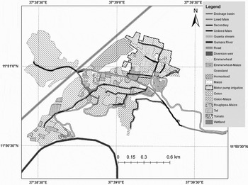
The study area, the Guanta small-scale irrigation scheme, is located in the highlands of the Blue Nile basin at a geographical coordinate of 11°50´N and 37°39´E at 1797 m asl in Ethiopia (Figure 1). It was selected based on accessibility, representativeness of small-scale irrigation in the study area and availability of information. A stone masonry diversion structure and 1555 m main canal (conveying water from the diversion) were constructed by the local government in 2001 while 850 m main canal and 1341 m secondary canal (conveying water from the main canal) was not yet lined. The layout of field canals (conveying water from the secondary canals to the individual fields) varied from time to time and it was difficult to map them. Other land units in the scheme were drainage basins and wetlands. Drainage basins were enclosed gully-like natural flood basins during the main rain rainy season. Farmers released excess irrigation water to these basins after irrigating their plots. On the other hand, wetlands were irrigated lands at the beginning of the scheme. These land units were changed to wetlands due to the overflow of water from the secondary canals and drainage basins. The irrigation scheme had an area of 90 ha, of which 21 ha was covered by pump irrigation at the upstream side of the main canal in 2009. A Water Use Association (WUA) was formed and rules for water price, canal maintenance and water allocation was established with the help of the government. However, not all were functional. The canals were not maintained on time, which changed their dimensions and geometry and caused uncertainty in calculating flow rates using other simple methods like ponding. Water allocation was done randomly mainly through agreements among some influential and wealthy farmers. Deneke (Reference Deneke2010) has reported an in-depth analysis on the group/village power on water allocation, lack of transparency in scheme boundary and land redistribution, rule enforcement mechanisms, theft and corruption.
Guanta small-scale irrigation scheme, highlands of the Blue Nile Basin, Ethiopia. ‘Ms’ shows the position of the canal discharge measurement stations.

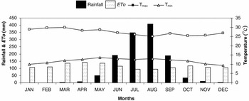
The main soil types in the scheme were Eutric Fluvisols and Eutric Vertisols (MoWR, Reference MoWR2008). In the present study, soil samples were taken at 0–50 cm and 50–100 cm depths for laboratory analysis and average soil characteristic values of each soil type were reported. The climate was characterized by mean annual rainfall of 1248 mm, mean maximum and minimum daily temperature of 27 °C and 12 °C, respectively. Climate data was obtained from nearby Bahir Dar and Woreta meteorological stations (Figure 2).
Average monthly rainfall (mm), monthly potential evapotranspiration (ETo) (mm), daily maximum temperature (Tmax) and minimum temperature (Tmin) (°C) for Guanta irrigation scheme 2009 (weather data from the nearby climatic station in Bahir Dar, (11°35´N, 37°23´E; 1798 m asl) and Woreta (14°40´N, 37°42´E; 1825 m asl).

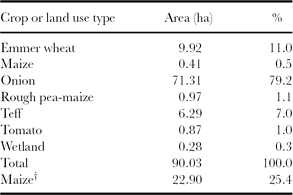
Farmers in the research site have been practicing mixed crop-livestock production systems. The average livestock holding was 3.2 TLU (tropical livestock unit, 250 kg live weight) per family and the stocking rate was 2.3 TLU per ha (Descheemaeker, personal communication, 2010). Feed shortage was severe in the flooded period of the main rainy season (Haileslassie et al., Reference Haileslassie, Peden, Gebreselassie, Amede and Descheemaeker2009b) when farmers commonly store crop residue to feed their livestock. Rice (Oryza sativa), finger millet (Eleusine coracana), maize (Zea mays) and teff (Eragrostis tef) were the main crops cultivated during the rainy season (June to September). After harvesting rice, rough pea (Lathyrus hirsutus) and chickpea (Cicer arietinum) were grown between October and December using the residual soil moisture. Onion (Allium cepa) was the main irrigated crop in the dry season (from January to May). Other crops like emmer wheat (Triticum dicoccum), called wheat hereafter, teff, maize and tomato (Lycopersicon esculentum) were of secondary importance in the irrigation scheme (Table 1). The cropping pattern in the irrigation scheme strongly depended on the availability of water and the market price. That means farmers' decision on what crop type and when to grow was based on their evaluation of the market conditions at harvest time. For example, in 2009 farmers opted for wheat (low yielding and high market valued variety) due to fear of market failure for onions as happened in the previous year (data not presented). Teff was a special crop in Ethiopia accounting for one-quarter of the cereal production and two-thirds of the protein in the national diet (NAS, Reference NAS1996). In addition, teff has soft, nutritious and palatable straw to feed livestock. A short-maturing teff variety (locally called Bukri and harvested within 47 days) was used by farmers during this study. About 79% of the scheme was covered by onion, 18% by wheat and teff, and 2% by grass lands around canals and wetlands during the 2009 irrigation season. About 25% of the scheme was covered by maize as a relay crop with onion.
Land use of Guanta small-scale irrigation scheme in the 2009 irrigation season (January–June).
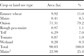
†Maize planted as a relay crop in onion fields, before the onion harvest.
Sampling and data collection
The fields, wetlands and canals of the scheme were mapped before determining the number and position of the sampling points. We used a Garmin e-trax Geographical Positioning System (GPS) and Satellite Pour l'Observation de la Terre (SPOT) satellite imagery from Google Earth (www.googleearth.com) to locate the study plots and to formulate a land use map of the scheme. Wetlands and drainage basins were delineated and their dimensions were measured. Irrigation canals were characterized as main, secondary or field canals. All fields were characterized as fed by pump or gravity irrigation. Unlined main and secondary canals had average grassland borders of 6.6 m wide (range 2.5–10.2 m). Throughout the irrigation season (January to May), we observed and mapped canal layout, canal maintenance, water distribution and water availability across the scheme's command area. We have conducted informal surveys using participatory rural appraisal tools, particularly informal group and individual discussions to understand major causes of water shortage and water loss, and upstream-downstream complexities from the perspective of local farmers.
To estimate biomass production, 11 irrigated fields were selected to represent the major crops cultivated in the scheme (four wheat fields, three onion fields and four teff fields) and to represent spatial distribution. At each selected field, a plot of about 400 m2 was delineated and pegged and the amount of applied water was measured as described later for each irrigation event from planting to harvesting. At harvest time crop biomass samples were taken from three 1 m2 plots distributed along the central line of each plot of teff and wheat. One of the wheat fields was very large and half of it missed one irrigation event. Therefore, six sample plots were taken for this field to address the farm size and irrigation variation within the field, so there were a total of 15 sample plots for wheat. Onion biomass was taken from 5 m furrow segments at 24 positions in each field from two gravity-irrigated fields and at 12 positions from one pump-irrigated field with a total of 60 sample furrow segments. Four fields were selected for data collection on maize relay cropping; however, the crop was destroyed by hail on 1 July 2009. Grass biomass, dominated by Cyprus rotundus and Cynodon dactylon, was sampled in ten 1 m2 plots along canals and within wetlands. During the irrigation season (about 120 days) the grass was repeatedly mowed from the sample plots (32 samples from canal boundaries, 38 samples from drainage basins and 14 samples from wetlands) when its height reached about 0.2 m. Each sample was dried to constant weight, and then grain, straw and grass biomass production were determined using a 0.001 kg sensitive balance. Crop residue production from grass, wheat and teff (covered about 20% land of the scheme) was calculated. According to FAO (1993) TLU dry matter (DM) need assessment study, 8.5 kg DM per TLU per day was used to quantify the number of TLU that could be fed during 60 days, assuming high feed shortage due to flooding for the whole main rainy season.
Canal flow measurements were taken at two points of a canal (100 m apart) to determine the amount of water lost through evaporation and seepage using inflow–outflow methods as described below. Continuous manual recordings of water levels were done twice monthly for four months, and every measurement took five hours. Replogle–Bos–Clemmens (RBC) flumes (Clemmens et al., Reference Clemmens, Bos and Replogle1984) were used to measure field canal loss and amount of water used to irrigate farm plots at every event throughout the irrigation season. Cutthroat flumes (Skogerboe et al., Reference Skogerboe, Bennett and Walker1973) of 0.91 m length and 0.41 m width were used to measure the water flow in the main and secondary canals. Manual water levels measured with the cutthroat flumes were transformed to flow rates using theoretical rating equations according to the manufacturer's manual (Eijkelkamp, undated). Although field installation and construction errors are always present, the weirs were selected for their greater accuracy (Clemmens et al. Reference Clemmens, Bos and Replogle1984; Eijkelkamp, undated; Skogerboe et al., Reference Skogerboe, Bennett and Walker1973) compared to other methods, such as like parshall flumes or the ponding method.
Data preparation and statistical analysis
Reference evapotranspiration (ET0) and crop water requirements were calculated using the Penman-Monteith and crop coefficient procedures described in Allen et al. (Reference Allen, Pereira, Reas and Smith1998). The database was formulated to use this procedure in order to minimize the uncertainty of using Bahir Dar stations. Therefore, rainfall and temperature data from Woreta and the relative humidity, wind speed and sunshine hours data from Bahir Dar meteorological stations were used to calculate reference evapotranspiration.
The water balance was calculated using the water balance equation (1) for the growing season at field level.

Where:
∆SM is the change in soil moisture content before the first irrigation and after harvest;
Peff is effective rainfall;
I is total irrigation water applied;
ET is actual evapotranspiration;
D is drainage loss;
Qr is capillary rise.
All quantities were defined within the same time domain (growing period) and units (mm water). Total irrigation need was computed using climate, crop and soil data using the FAO CROPWAT version 8.0 (FAO, 2009). ∆SM was calculated as the difference between soil moisture content before the first irrigation and soil moisture content after harvest. Soil moisture data were determined using a gravimetric method with dry bulk density data adopted from MoWR (2008). Peff was calculated using United States Department of Agriculture's Soil Conservation Service empirical formula. It was selected from the three options found in CROPWAT 8.0 software as it was developed for long-term climatic and soil moisture data (FAO, 1978). ET was calculated by multiplying the crop coefficient (Kc) with water stress factor (Ks). Ks is a function of total available water (TAW), readily available water and root zone depletion. It was estimated from daily water balance computation (Allen et al., Reference Allen, Pereira, Reas and Smith1998). The crop parameters like crop growth stages, allowable depletion factor, Kc, and rooting depth were adopted from Allen et al. (Reference Allen, Pereira, Reas and Smith1998). Length of cropping season was taken from the field data. Since teff is a local crop without these important parameters in the literature, grass values were adopted for it. Grass Kc values are also almost similar to average values of cereal crops. The crop coefficient for the grasslands around canals, drainage basins and wetlands was formulated using mean values of legumes and grasses previously reported (Haileslassie et al. Reference Haileslassie, Peden, Gebreselassie, Amede, Wagnew and Taddesse2009a; Reference Haileslassie, Peden, Gebreselassie, Amede and Descheemaekerb). Drainage loss was calculated as the sum of irrigation water that was applied above field capacity at every irrigation event. Therefore, the drainage loss was not supposed to mean the difference between irrigation water applied and irrigation water required. Capillary rise was not considered, as the ground water table was more than 2 m deep (Allen et al. Reference Allen, Pereira, Reas and Smith1998; MoWR, 2008). Soil physical characteristics, such as bulk density and TAW content, were adopted from MoWR (2008) as the data was generated from the same scheme. Field capacity was calculated from TAW and root depth.
Canal or conveyance loss (in l s−1 100 m−1 canal length) was calculated as presented in equation 2 using inflow–outflow methods. This method was selected since it was difficult to determine canals geometry and canal parameters as described in the study area.

Where:
Qin is water flow rate at the upper side of 100 m long canal segment (measured);
Qout is water flow rate at the lower end of 100 m long canal segment (measured).
Canal water loss was calculated as the percentage of conveyance loss to the average of Qin and Qout with in 100 m canal segments. From field observations, data on total canal length and water loss per 100 m, an average of 30 l s−1 water was reached at the end of secondary canals and distributed to many field canals at the same time. Therefore, measured canal loss was converted to this average water flow rate for comparison.
Water productivity along canals and in irrigated fields was calculated using equations 3 and 4.


Irrigation and actual ET water productivity were calculated for both grain and dry straw biomass using two approaches. The ‘conventional approach’ considers all the water supplied by irrigation and depleted by ET to compute grain or straw (but not for both) biomass water productivity while for an ‘improved approach’ we followed Haileslassie et al. (2009a;b), which computed water productivity using the water supplied by irrigation and water depleted by ET for total biomass (both grain and straw) production. Therefore, yield of the system at the numerator side of the equations is larger than the conventional way of calculation. This approach reflects the real situation on the ground in which both straw and grain were using the same ET water for producing feed and food, respectively. Both approaches, hereafter termed as ‘conventional’ and ‘improved’ were used for comparative estimation of water productivity.
Relative water supply (RWS), a performance indicator, was calculated using equation 5 taken from Levine (Reference Levine1982). It is the ratio of total water supplied by irrigation (I) and rainfall (P) to total water demanded by crop (i.e. actual crop evapotranspiration, ET).
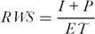
Relative water supply was calculated for the growing season for selected crops for both gravity and pump irrigation.
After the field data were processed using the above procedures, statistical analysis was conducted using descriptive statistics, one-way analysis of variance, which compares groups sample means with one factor at a time (SPSS, 2004), for the three crop types and t-test for gravity and pump irrigation types. Means were compared using the least significant difference test at significant level, p ≤ 0.05.
RESULTS
Water loss and grass production around canals and wetlands
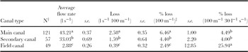
The highest water loss rate in l s−1 100 m−1 was observed from the main canal while the lowest was from field canals (Table 2). The highest daily volume of water was lost from the field canals when we assumed 30 l s−1 flow rate for all canal types. Calculations of the loss for the total amount of flowing rate (30 l s−1) showed that about 26% of the water in the field canals was lost. This loss was much lower for the main and secondary canals at 4.49% and 4.00%, respectively (Table 2).
Canal water losses due to water surface evaporation and seepage from Guanta small-scale irrigation scheme.

†Number of observations.
‡Percentage with respect to the seasonal average flow rate with in each canal type.
Values indicated by the different superscript letter are significantly different at p ≤ 0.05.
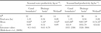
Grasslands and wetlands were part of the irrigation scheme and consumed irrigation water while producing biomass. The grasslands produced grass biomass using seepage water from the canals. Wetlands were formed under influence of excess drainage water and freely released water from irrigated fields. Wetlands and drainage basins were not observed in the motor pump irrigation area. The ET water productivity of grassland varied with farm positions from 0.4 to 1.2 kg m−3, which was below the productivity of rain-fed wetlands (Table 3). The grassland in the drainage basin was the most productive, whereas the wetland had the lowest productivity. The land productivity was quite high, ranging from 3000 to 9000 kg ha−1 (Table 3). Although grass production can be considered as a productive use of the water lost through canal seepage, only about 0.05% of the water lost from the canals was actually used for grass production. The other part was lost through canal storage, deep drainage, water surface evaporation and flow back to the river system.
Seasonal water productivity and land productivity of grasslands along earthen canals, in drainage basins and in wetlands in Guanta irrigation scheme for the 2009 irrigation season.

†Grassland along canals; ‡wetland due to drainage water; §wetland due to overflow of irrigation water; ¶Number of biomass samples taken with in the season.
Values indicated by the different superscript letter are significantly different at p ≤ 0.05.
Comparative performance indicator: relative water supply
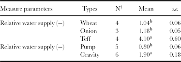
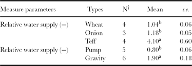
Relative water supply, reflecting the availability of water in relation to crop demand, was 1.04 and 1.18 for wheat and onion, respectively (Table 4), indicating that the total water applied was similar to the crop needs. With a significantly different RWS value of 4.1, the average water applied for teff was four times higher than the requirements, and ranged up to seven for certain plots. Teff had a much higher variation in RWS as compared to wheat and onion (p ≤ 0.05.)
Relative water supply for different crops and irrigation types.
†Number of observations.
Values indicated by the different superscript letter are significantly different at p ≤ 0.05.
Relative water supply was significantly lower (p ≤ 0.05) for motor pump than for gravity irrigation: RWS was 0.5 and 1.35 under pump and gravity irrigation, respectively, for onion while the other two crops were not planted in both gravity and pump irrigation types to have this comparison. This indicated that farmers under-irrigated their farms when they are using pumps and over-irrigated when they are using gravity irrigation.
Crop production and productivity
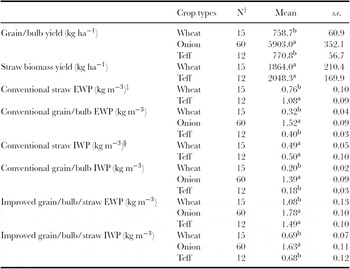
Productivity analysis revealed that grain biomass yield for teff and wheat was very similar at 770 and 759 kg ha−1, respectively, whereas straw yield was slightly higher for teff at 2048 kg ha−1 compared to 1864 kg ha−1 for wheat (Table 5). The onion yield was 5903 kg ha−1. Water productivity was higher for onion than for the cereals. On the other hand, IWP of crops was less than EWP for both water productivity approaches, for all crops, and for grain/bulb as well as for crop residues due to irrigation water application losses. Due to high application loss onion and teff had statistically similar EWP while they had statistically different IWP. Conventional IWP ranged from 0.18 to 1.39 kg m−3 while improved IWP ranged from 0.68 to 1.78 kg m−3 (Table 5).
Yield and water productivity of main crops in Guanta irrigation scheme.

†N: number of observation; ‡EWP: evapotranspired water productivity; §IWP: irrigation water productivity.
Values indicated by the different superscript letter are significantly different at p ≤ 0.05.
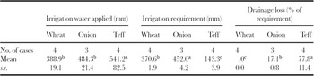
In addition to RWS, the amount of irrigation water application and amount of crop water need showed that the total amount of irrigated water did not match that needed by crops especially for teff: the water input was much higher than the evapotranspiration water requirement. The irrigation water requirement and water application varied greatly among the selected crops. The irrigation water requirements of the crops were significantly different (p ≤ 0.05), but farmers applied almost equal amount of water for wheat and onion. As a result, strong variation (p ≤ 0.05) in irrigation water losses (ranging from 0 to 78% of the required water) due to over-irrigation was observed between the crop types (Table 6). Wheat was not irrigated beyond field capacity and no irrigation loss was observed. Farmers irrigated wheat and teff two to three times within the growing season while onion was irrigated seven to eight times. The short-maturing teff variety can produce grain and straw within 47 days, requiring the lowest irrigation water amount. However, farmers applied most water to teff fields resulting in the highest water loss (78% of the required water or 30% of the applied water was a drainage loss) and the lowest irrigation water productivity (Table 6). High water application for teff occurred because of the flood irrigation method and crack formation at each irrigation event.
Irrigation water application and requirement for different crops in Guanta irrigation scheme.

Values indicated by the different superscript letter are significantly different at p ≤ 0.05.
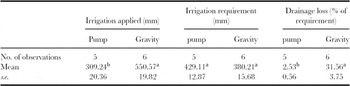
Farmers at the upstream side of the gravity-fed scheme invested in motor pumps, fuel and technicians to pump water to their fields. Farmers with land but without pumps shared half of their produce with those providing pumped water. However, water from gravity irrigation was free. As a result, strong differences in amounts of applied water were observed for pump and gravity irrigation (Table 7). Even though crops needed similar amounts of water whether irrigated by pump or gravity (the small difference was observed due to difference in crop type and plantation and harvest time), farmers applied more water to gravity-irrigated crops than to pump-irrigated ones. Consequently, pump-irrigated crops were under-irrigated while gravity-irrigated crops were over-irrigated (Table 7). Even though there was overall under-irrigation during pump irrigation, in some cases excess water was applied above soil field capacity. As such, about 3.4% of the applied water or 2.5% of the required water was lost due to drainage (Table 7).
Irrigation water application and requirement for pump and gravity irrigation.

Values indicated by the different superscript letter are significantly different at p ≤ 0.05.
Discussion with farmers revealed that there was an increasing irrigation water demand (data not presented). The diversion and main canal capacity was designed for 46 ha. However, about 20 ha of an additional farm land was included by the farmers at the tail end of the scheme. In addition, farmers in the upstream irrigate 21 ha of land using motor pipes, which was not originally part of the scheme. Increasing water demand by both upstream and downstream communities aggravated the water shortage leading to prolonged irrigation intervals. As a result, the soil was deeply cracked in many locations, leading to high losses of irrigation water due to water percolation through the cracks.
DISCUSSION
This study indicated that irrigation cost had its implications on water management decision and variations in water productivity. Production costs associated with pump irrigation forced farmers to save water and to frequently maintain canals, which was evidenced by the absence of water draining away from the fields. Farmers minimized water losses by using deficit irrigation and by transferring water immediately to the next plot. On the other hand, over-irrigation and high water losses were observed on fields irrigated by gravity-fed water. In that part of the irrigation scheme, farmers were reluctant to maintain canals appropriately and water was released to the drainage basin in spite of high water need at the tail. The difference of water requirement for the same crop came from differences in planting and maturity time in different fields.
Irrigation water losses and shortage: cause, effects and possible mitigation
Higher small-scale irrigation canal water loss was observed in our study when compared to the findings of Akkuzu et al. (Reference Akkuzu, Unal and Karatafi2007) who reported about 9.3% average loss from lined field canals and 1.1% loss from lined secondary canals in Turkey at similar 30 l s−1 flow capacity. Bakry and Awad (Reference Bakry and Awad1997) reported 0.17 to 0.70% per 100 m canal loss in Egypt for canal capacity of 2000 to 12 100 l s−1, which was also lower than our values. The canal water loss in our study was highest from the main canal due to its higher capacity (43.21 l s−1) and proximity to the river bank, as compared to the other canal types. Expressed as percentage of the water flow capacity of the canals, the canal loss was highest for the field canals, since these were destroyed during tillage, so that the canal banks were not stabilized like the main and secondary canals. The negative impact of seepage on production was more pronounced in the case of field canals as it led to more water logging than the seepage from other canals.
In addition, the field canal network covered the biggest portion in the scheme. Farmers preferred field canals because it allowed them to keep their plot sizes. Apart from high seepage losses, field canals dried and cracked before the next irrigation. Field canals overtopping during night irrigation was common and increased water logging and unmeasured canal water loss. All these resulted in large irrigation water loss, water logging and production losses. Therefore, large farmlands within 8–15 m from the field canals were out of production. Although farmers thought secondary canals occupied more land than field canals, in practice field canals rendered more land unproductive and resulted in higher water losses than did secondary canals. The total volume of water lost from the 3077-m long canal system (comprising all canal types) could have irrigated 9 ha of land at 50 mm irrigation depth per day.
The increasing water demand due to the extension of tail and pump irrigation have made the management of the irrigation water more complicated. The duration of the irrigation intervals increased, which resulted in crop water stress and cracks in the vertic soils. In addition, due to decreased canal flow capacity, the time needed for sufficient irrigation increased and farmers were forced to conduct night-time irrigation, resulting in large losses due to inefficiency and unpredicted canal flow rate during the night.
Water was a more constraining factor than land around the scheme during the irrigation season. Ample downstream plain land was out of production six months a year (December to June). On the other hand, water from night stream flow, springs and shallow ground water was still not used properly. A simple profile leveling survey of the Guanta river showed great potential for night water storage (up to 20 000 to 45 000 m3), which could be used at daytime. Farmers invested about 50% of their produce in kind for pump irrigation, with an increasing trend of pumping activities. However, because of higher production costs, pump irrigation typically resulted in lower financial water productivity than downstream gravity irrigation. That means, there is a stronger possibility to improve water productivity in downstream gravity irrigation than upstream pump irrigation.
The variation in RWS indicated that more water was lost for teff and under gravity irrigation and values ranged from 0.8 to 4.0, where 0.8 indicated deficit irrigation to maximize water productivity (Molden et al., Reference Molden, Sakthivadivel, Perry, de Fraiture and Kloezen1998). In a public surface irrigation scheme in Mexico, RWS was higher than 2.0 and showed differences with respect to water access and water cost (Kloezen and Garcés-Restrepo, Reference Kloezen and Garcés-Restrepo1998). Compared to the above study which used RWS at scheme level, RWS for teff was extremely high.
Land and water production and productivity
Area and water productivity of selected crops was comparable with findings of other studies around the study area. Haileslassie et al. (Reference Haileslassie, Peden, Gebreselassie, Amede and Descheemaeker2009b) reported yields of 892–972 kg ha−1 for wheat and 981–1312 kg ha−1 for teff produced in rain-fed conditions in the same watershed. The EWP values were 0.21–0.23 kg m−3 for wheat and 0.24–0.33 kg m−3 for teff in the study of Haileslassie et al. (Reference Haileslassie, Peden, Gebreselassie, Amede and Descheemaeker2009b) that used the improved approach of water productivity calculation. This showed that land productivity was relatively smaller while the water productivity was three times higher in our study as compared to Haileslassie et al. (Reference Haileslassie, Peden, Gebreselassie, Amede and Descheemaeker2009b). The difference observed between these rain-fed and irrigation results arose from differences in crop varieties and water management practices. On one hand, short-maturing teff and wheat varieties with lower ETc were used for irrigation than for rain-fed production. On the other hand, irrigation intervals were too long to create soil water stress conditions whereby water stress coefficient was reduced to 0.3 during some irrigation intervals. Bekele and Tilahun (Reference Bekele and Tilahun2007), using experimental deficit irrigation at Sekota, obtained 5500–25 000 kg ha−1 and 9–10 kg m−3 for onion, which is about eight times higher than our observations. This showed that there were opportunities to increase onion production and productivity of the area. Flood irrigation using very low flow rate (less than 1 l s−1 during the night or day) and irrigating deep cracks after prolonged irrigation intervals decreased the water productivity of teff and wheat as compared to the field observation on water application. For example, teff irrigation water was almost half as productive as ET water compared to wheat and onion productivities due to higher drainage water losses.
The conventional way of quantifying water productivity underestimated water productivity values since the total water transpired was used to produce total biomass while the estimation considered either grain or straw. This approach has more practical application in mixed crop-livestock system whereby the straw biomass is a very important livestock feed.
Implication on livestock production
As the importance of crop production on livestock is worth considering, it is also important to stress the importance of crop residue as livestock feed during the irrigation season. About 11 428 kg grass, 18 490 kg wheat straw and 12 884 kg teff straw (42 884 kg DM in total) were produced from 18 ha (20%) land of the scheme within the season. Using 8.5 kg DM per day maintenance need for a TLU, 84 TLU can be fed for 60 days. This can cover TLU from 26 households or TLUs that cover 37 ha according to the livestock holding and stocking rate of the area studied by Descheemaeker (personal communication, 2010). Dry matter production from the relay maize cropping and other minor crops of the scheme was not considered in this calculation, and the potential of the scheme to support livestock feed is expected to exceed the above indicated figures. Therefore, increasing the biomass productivity of each drop of irrigation water and at each plot of land within the scheme has strong implication on livestock water productivity of the mixed crop-livestock systems.
RECOMMENDATIONS
1. Based on the above findings, recommendations for improving water use efficiency and productivity in the irrigation scheme include careful design and construction of secondary canals and decreasing the use of field canals to minimize canal water loss. Careful planning of the cropping pattern and irrigation scheduling could result in more efficient water distribution. Given the fact that over-irrigation is less common with pumped irrigation, allocating a water price to gravity-fed water could positively influence water management. However, water pricing has to be based on accurate water flow data as well as equitable, adequate and reliable water distribution rules governed by the water user associations. Water flow measurements can be conducted using cement, wooden or iron sheet cutthroat flumes by trained farmers.
2. Production of high value crops (e.g. fruits) and/or high quality feeds along canals and drained water could maximizes water productivity for livestock, and there is an opportunity to increase irrigation water productivity.
3. In order to improve water productivity of these system, farmers, water users associations and development agents should receive training on canal water management, crop water requirement, and equitable and efficient water distribution.
4. Different alternatives for improved water management, such as water pricing and facilities for night water storage need to be considered in policy development.
5. Considering the trade-offs between downstream gravity irrigation and upstream pump irrigation needs further research for supporting policy articulations.
6. Shallow and frequent irrigation of teff using sprinkler or border irrigation could minimize water loss and increase irrigation water productivity, but needs further research on the applicability in the local context.
Acknowledgements
This study was performed as part of the project entitled ‘Improving Water Productivity of Crop-Livestock Systems of Sub-Saharan Africa’. We thank the International Water Management Institute (IWMI) and German Federal Ministry for Economic Development Cooperation (Bundesministerium Für Wirtschaftliche Zusammenarbeit-BMZ) for covering research costs. We also thank Dr Selamyihun Kindu and Amhara Agricultural Research Institute (ARARI) for providing RBC flumes and advice, Sirinka Agricultural Research Center (SARC) for providing automatic rain gauges, Ethiopian Meteorological Agency for providing meteorological data, and Solomon Ewnetu and Habtamu Tensae for collecting field data.