Across a broad range of fields in political science, there are many theoretically interesting dependent variables that can be characterized as compositions. The vote shares of competing political parties and the shares of budgets allocated to different spending categories are two of the most prominent examples. Researchers have long recognized the complications that compositional data pose and have implemented strategies developed by statisticians and researchers in other fields to test their hypotheses about such variables with cross-sectional data.
More recently, researchers have adapted these modeling strategies to dynamic contexts where they have measured values of a compositional dependent variable over multiple time points for the same spatial unit. These approaches represent substantial improvements over previous strategies for dealing with such dependent variables, which either oversimplified the compositional nature of these data or ignored the possibility that dynamic relationships shaped them. However, even fully dynamic compositional models are limited, because they do not allow for the analysis of theoretically interesting variation across both time and spatial units. This means that researchers cannot get leverage on the effects of variables that do not vary much or at all within a single time series. As a multitude of recent papers have demonstrated, there is abundant evidence that what is happening in one spatial unit often affects what happens in other spatial units, especially those that are closely linked together through geography or other factors (Beck, Gleditsch and Beardsley Reference Beck, Gleditsch and Beardsley2006; Franzese and Hays Reference Franzese and Hays2007; Neumayer and Plümper Reference Neumayer and Plümper2012; Darmofal Reference Darmofal2015).
In this paper, we build on previous work in two ways. First, we develop a strategy for adapting dynamic compositional models to time series cross-sectional contexts in which we can model the effects of contextual and spatial relationships across units. We do this by extending the modeling strategy developed by Philips, Rutherford and Whitten (Reference Philips, Rutherford and Whitten2016a). Second, as modeling strategies for compositional dependent variables produce non-linear estimated relationships and most of them produce copious statistical output, graphical techniques for interpretation have been quite popular. Therefore, we also present a series of new graphical strategies to help with the interpretation of the results from models of compositional variables over time and space.
In the next section, we provide a brief discussion of the analysis of compositional dependent variables over time and discuss a series of extensions of these models to data that vary across both time and space. We then provide a methodological illustration of these extensions using budgeting data from the US states. Finally, we include a discussion of our contributions and some possible future directions.
MODELING COMPOSITIONAL DEPENDENT VARIABLES OVER TIME
There has been a growing body of work on dynamic compositional dependent variables in political science in recent years. Examining government responses to fiscal austerity in 21 OECD countries, Breunig and Busemeyer (Reference Breunig and Busemeyer2012) model relative changes between budgetary categories. As they state, explicitly modeling trade-offs between categories moves closer to the “empirical reality of governmental decision-making, where policy-makers are constantly faced with decisions on how to allocate scarce public resources across budget categories” (Breunig and Busemeyer Reference Breunig and Busemeyer2012, 923). Such a modeling strategy was substantially extended by Philips, Rutherford and Whitten (Reference Philips, Rutherford and Whitten2015, Reference Philips, Rutherford and Whitten2016a), who advocate for the use of graphical depictions of counterfactual “shocks” to variables of substantive interest.
Since compositional data have many unique qualities, it is worth describing them in some detail. Consider a compositional dependent variable, Y, that consists of C components.Footnote
1
Individual observations of each component at each point in time, y
ct
, have the same four defining characteristics.Footnote
2
First, each component of the composition has a value between 0 and 1 (0<y
ct
<1). Second, the components sum to one at each point in time
 $( {\mathop{\sum}\nolimits_{c\,{\equals}\,1}^C {y_{{ct}} } \,{\equals}\,1\,\, \forall t} )$
.Footnote
3
Third, any change in a single component is bounded by −1 and 1 (−1<∆y
ct
<1). Fourth, all changes among component parts at any single point in time must sum to 0
 $( {\mathop{\sum}\nolimits_{c\,{\equals}\,1}^C {\Delta y_{{ct}} } {\equals}\,0} )$
.
When C=2, models with y ct can be estimated with an ordinary least squares (OLS) regression model.Footnote 4 When C>2, matters become considerably more complicated. As Aitchison (Reference Aitchison1982, Reference Aitchison1983, Reference Aitchison1986) demonstrated, any modeling approach that assumes independence across the columns of Y will be problematic. Following Aitchison, for a compositional dependent variable, y ct , with C components and a chosen reference category, c=1, we can calculate C−1 logged ratios, which we label s ct , such that
 $$s_{{ct}} \,{\equals}\,{\rm ln}\left( {{{y_{{ct}} } \over {y_{{1t}} }}} \right)\quad \forall c\,\ne\,1.$$
We then can estimate the effects of independent variables in each of the C−1 equations, because one of the categories, y 1t , becomes the “baseline” for all the log-ratios; the choice of baseline category is arbitrary.
The modeling strategy proposed by Philips, Rutherford and Whitten (Reference Philips, Rutherford and Whitten2016a) to test theoretical claims about compositional dependent variables with more than two categories in models for a single spatial unit over time is given as
 $$\Delta s_{{ct}} \,{\equals}\,\beta _{{0c}} \,{\minus}\,\alpha _{c} s_{{c,t{\minus}1}} {\plus}{\bibeta }_{{Lc}} {\bf x}_{{t{\minus}1}} {\plus}{\bibeta }_{{Sc}} \Delta {\bf x}_{t} {\plus}{\varepsilon}_{{ct}} ,$$
where ∆s ct is the change in the logged ratio of dependent variable category “c” for c>1 relative to baseline category c=1 from time “t−1” to time “t,”Footnote 5 x t a vector of independent variable values at time “t,” −α c the adjustment parameters that measure the long-run error correction processes, β sc a vector of short-run effects, β Lc a vector of parameters that can be combined with −α c to calculate estimated long-run effects of changes in each independent variable,Footnote 6 and ε ct a stochastic disturbance term that may be correlated across the C−1 equations.
As is clear from Equation 2, Philips, Rutherford and Whitten (Reference Philips, Rutherford and Whitten2016a, Reference Philips, Rutherford and Whitten2016b) recommendation is for a system of error correction equations, and the advantage of this approach is that it estimates both the short- and long-run effects of changes in any of the independent variables. Because of the extensive parameterization from such models, these authors recommend the use of graphical simulations for the interpretation of the estimated relationships; we build on their work along these lines below.
EXTENDING DYNAMIC COMPOSITIONAL MODELS ACROSS SPACE
We can gain leverage on a wide range of concepts of theoretical interest by extending the dynamic compositional models proposed by Philips, Rutherford and Whitten (Reference Philips, Rutherford and Whitten2016a) to time series cross-sectional data. In this section, we provide an overview of the details of how we can adapt these modeling strategies from models of single spatial units over time. As a first step, we adjust the system of equations represented in Equation 2 by adding an “i” subscript for different spatial units such that our equation becomes
 $$\Delta s_{{ict}} \,{\equals}\,\beta _{{0c}} \,{\minus}\,\alpha _{c} s_{{ic,t{\minus}1}} {\plus}{\bibeta }_{{Lc}} {\bf x}_{{i,t{\minus}1}} {\plus}{\bibeta }_{{Sc}} \Delta {\bf x}_{{it}} {\plus}{\varepsilon}_{{ict}} .$$
Models of time series cross-sectional data have become prevalent in nearly all subfields of political science. Two of the biggest attractions of this broad class of models are that they allow researchers to gain leverage on the impact of contextual independent variables that do not vary much (or at all) within single spatial units over time (e.g., Plümper and Troeger Reference Plümper and Troeger2007; Clark and Linzer Reference Clark and Linzer2015) and that they allow researchers to model the impact of spatial processes in which aspects of what is happening in unit “j” affect the dependent variable in unit “i” (e.g., Beck, Gleditsch and Beardsley Reference Beck, Gleditsch and Beardsley2006; Franzese and Hays Reference Franzese and Hays2007). Our main goal is to show how researchers can accomplish both of these tasks when the dependent variable is a composition. For ease of exposition, we first discuss the incorporation of spatial factors and then proceed to consider the inclusion of interactive contextual factors.
Recent literature on spatial statistical models has advocated the spatial-X model as a good starting point for testing theories about spatial effects (Halleck Vega and Elhorst Reference Halleck Vega and Elhorst2015). Although we also consider spatially lagged (i.e., spatial-Y) models below, we find this setup particularly attractive due its flexibility in terms of model specification and the ease with which researchers can estimate it. We can incorporate theoretically interesting spatial effects through the inclusion of a set of θ WZ terms
 $$\Delta s_{{ict}} \,{\equals}\,\beta _{{0c}} \,{\minus}\,\alpha _{c} s_{{ic,t{\minus}1}} {\plus}{\bibeta }_{{Lc}} {\bf x}_{{i,t{\minus}1}} {\plus}{\bibeta }_{{Sc}} \Delta {\bf x}_{{it}} {\plus}\bitheta _{{Lc}} {\bf WZ}_{{t{\minus}1}} {\plus}\bitheta {\bf W}\Delta _{{Sc}} {\bf Z}_{t} {\plus}{\varepsilon}_{{ict}} ,$$
where θ is a vector of spatial parameters to be estimated, W the theoretically specified weights matrix connecting our spatial units, and Z a matrix of variables with values for other spatial units (j≠i) that are expected to work through θ and W to affect s ict . Presently, we are interested in testing theories about two types of spatial effects: spillover effects and spatial diffusion/contagion effects. For spillover effects, we populate our Z matrix with contemporaneous or lagged values of selected variables from x, and we provide an example of this type of effect below. Readers familiar with spatial statistical models will recognize this model, regardless of the variables included in Z, as a spatial-X (SLX) model.Footnote 7 In order to estimate spatial diffusion/contagion effects, we use s jct values to estimate a spatial autoregressive (SAR) model. As recent work has demonstrated, for both types of models, the specification of W must be done based on theoretical expectations about how changes in surrounding spatial units affect each other (Neumayer and Plümper Reference Neumayer and Plümper2012).
As outlined above, another attractive reason for extending these models to the pooled time series setting is that it gives us the ability to test for the impact of contextual variables such as institutions, government partisanship, and other variables that do not usually vary much within a single time series. If we theorize that these variables work in an additive fashion, they can appear in our models as just another element in x. However, we often expect these variables to work through the other independent variables to affect the phenomena being modeled. Following the example of Philips, Rutherford and Whitten (Reference Philips, Rutherford and Whitten2015), we can model the effects of such variables with a dichotomous indicator, d it , that we interact with the theoretically relevant right-hand side variables in our models.Footnote 8 To apply this to a setting that also includes the spatial effects (as depicted in Equation 4), we first collect the lagged dependent variable s ic,t−1 and the vector of parameters for the lagged independent variables and express them as a function of the adjustment parameter α c
 $$\Delta s_{{ict}} \,{\equals}\,\beta _{{0c}} \,{\minus}\,\alpha _{c} (s_{{ic,t{\minus}1}} {\plus}{\bf \kappa }_{{Lc}} {\bf x}_{{it{\minus}1}} {\plus}{\biomega }_{{Lc}} {\bf WZ}_{{t{\minus}1}} ){\plus}{\bibeta }_{{Sc}} \bDelta {\bf x}_{{it}} {\plus}{\bitheta W}\Delta _{{Sc}} {\bf Z}_{t} {\plus}{\varepsilon}_{{ict}} ,$$
where
 $${\bibeta }_{{Lc}} \,{\equals}\,{{{\minus}{\bikappa }_{{Lc}} } \over {\alpha _{c} }}$$
and
 $${\bitheta }_{{Lc}} \,{\equals}\,{{{\minus}{\biomega }_{{Lc}} } \over {\alpha _{c} }}$$
. We then add the term
 $$d_{{it}} \phi _{c} $$
to the adjustment parameter and
 $$d_{{it}} \zeta _{c} $$
to the short-run parameters to change our system of equations to
 $$\Delta s_{{ict}} \,{\equals}\,\beta _{{0c}} {\minus}\alpha _{c} (1{\plus}d_{{it}} \phi _{c} )(s_{{ic,t{\minus}1}} {\plus}{\bf x}_{{i,t{\minus}1}} {\bikappa }_{{Lc}} {\plus}{\biomega }_{{Lc}} {\bf WZ}_{{t{\minus}1}} ){\plus}(1{\plus}d_{{it}} \zeta _{c} )(\Delta {\bf x}_{{it}} {\bibeta }_{{Sc}} {\plus}{\bitheta W}\Delta _{{Sc}} {\bf Z}_{t} ){\plus}{\varepsilon}_{{ict}} .$$
This specification allows both the short- and long-run adjustments to vary depending on the value of d it . When d it =0, Equation 6 reverts back to Equation 5.
In the next section, we show an example of a model estimated with both spatial effects and partisan effects, which we measure with a d it term. To help interpret these effects, we develop figures that depict the substantive changes that are a consequence of simulated changes to the values of an independent variable.
METHODOLOGICAL ILLUSTRATION: BUDGETING IN US STATES
As a methodological illustration of the modeling strategies discussed above, we conducted an analysis of the role of partisanship in shaping the annual budgets of the 48 contiguous US states. We collected data for this example from the US Census Annual Survey of Government Finance from 1977 to 2008. This survey provides information on major revenue and expenditure categories for each state in current dollars for a fiscal year (e.g., 1992 would reflect expenditures for the fiscal year spanning 1 July 1991 and 30 June 1992). Data are compiled from state government budgets, audits, and additional financial reports, which the Census Bureau compiled and reassigned to classification categories to make them directly comparable.
The dependent variable consists of five components, expressed as proportions, that define direct expenditures by function in each state across time: education, social services (i.e., public welfare, hospitals, and veterans services), public services (transportation, public safety, and housing), labor market policy, and a collection of smaller categories which we lumped together as “Other.”Footnote 9 As these are compositional data, all five components sum to 1 in each year for each state.
For our independent variables in this example, we relied on collections of data from Klarner (Reference Klarner2013a, Reference Klarner2013b) and the Bureau of Economic Analysis. We present results from a relatively parsimonious model in which the independent variables are average real state personal income, the rate of unemployment in the state, the rate of unemployment in other states, and the partisanship of the state governor. In this model, the unemployment rate in other states is our spatial variable, referenced as Z in Equations 4 through 6. Our expectation is that unemployment in other states is seen as a harbinger of tough economic times and thus leads politicians to adjust their budgets in expectation of future changes. In thinking about how unemployment in other states is likely to affect budgeting in each state, we expect this to be a function of two factors: geographic proximity and economic size relative to all other states. We thus constructed a weights matrix, W, that is the product of two different weights matrices:
 $${\bf W}\,{\equals}\,\left( {{\bf W}_{{1/{\rm dist}}} \cdot {\bf W}_{{{\rm row\,{\minus}\,std}{\rm .Econ}}} } \right),$$
where W row−std.Econ is a row-standardized weights matrix of each state’s contribution to national personal income, which we pre-multiply by W 1/dist, that is an un-standardized inverse distance matrix (such that states that are further away get lower weights).Footnote 10 This specification reflects our theoretical expectations; for example, even though Oregon is geographically more proximate to the state of Washington than California, California’s dominant economic influence in the region likely means that changes in economic conditions in that state are still substantial in Washington. Thus, this weights matrix specification takes into account both distance and economic influence.
In this example, we model gubernatorial partisanship as our contextual factor, referenced as d it in Equation 6. Here, d it =1 if the current governor is a Democrat and 0 otherwise.Footnote 11 We are thus allowing the effects of all of our other independent variables on budgeting to differ depending on the partisanship of the state’s governor.
Results using a model specified according to Equation 3 produce a heavy parameterization; the five dependent variable categories create four compositional trade-offs with 16 parameters (plus a constant) in each equation.Footnote
12
Instead of presenting a table of parameter estimates, we follow the current convention of presenting the results from dynamic simulations (Williams and Whitten Reference Williams and Whitten2011, Reference Williams and Whitten2012; Philips, Rutherford and Whitten Reference Philips, Rutherford and Whitten2016a, Reference Philips, Rutherford and Whitten2016b).Footnote
13
More specifically, we follow the lead of Philips, Rutherford and Whitten (Reference Philips, Rutherford and Whitten2016a) and present figures depicting “change from baseline” simulation scenarios. To obtain the quantities for these figures, we first estimate each of the C−1 equations in a seemingly unrelated regression framework using the Clarify program developed by Tomz, Wittenberg and King (Reference Tomz, Wittenberg and King2003). Estimating compositional variables in a seemingly unrelated regression is ideal due to the potential for contemporaneous correlation of errors, as well as the fact that the components must sum to one (Jackson Reference Jackson2002; Mikhailov, Niemi and Weimer Reference Mikhailov, Niemi and Weimer2002; Tomz, Tucker and Wittenberg Reference Tomz, Tucker and Wittenberg2002).Footnote
14
Next, after creating posterior densities of our parameter estimates through 1000 sets of simulations, we set the lagged dependent variable of each category to its sample mean,
 $$\bar{Y}_{c} $$
. The differenced independent variables are set to 0, while the lagged independent variables are set to their sample means. We then take the expected value of each of our dependent variables at time t. This becomes the new value of the lagged dependent variable at time t+1. This process is repeated until period 4, when we change one of the differenced independent variables of interest by one standard deviation. In period 5, the differenced independent variable becomes 0 again, and the “shock” gets added to the mean of the respective lagged independent variable. After 20 iterations, we save the results and un-transform the
 $$\hat{s}_{{ijt}} $$
values to yield the expected proportion of each category, along with 95 percent confidence intervals calculated using the percentile method. The formula for the un-transformation is
 $$\hat{y}_{{ijt}} \,{\equals}\,{{e^{{\hat{s}_{{ijt}} }} } \over {1{\plus}\mathop{\sum}\nolimits_{c\,{\equals}\,2}^C {e^{{\hat{s}_{{ijt}} }} } }}\forall c\,\gt\,1,$$
and
 $$\hat{y}_{{ijt}} \,{\equals}\,{1 \over {1{\plus}\mathop{\sum}\nolimits_{c\,{\equals}\,2}^C {e^{{\hat{s}_{{ijt}} }} } }},$$
for the baseline category. The resulting output is then graphed over time around the expected value of the individual dependent variable categories in each of the simulated time periods with surrounding confidence intervals.Footnote 15
By treating every compositional equation as part of a broader system (i.e., the entire budget), we are able to gain a rich set of big picture inferences. In addition, we are able to overcome one of the major difficulties in graphically presenting results from analyses of compositional dependent variables using traditional simplex and/or ternary plots. These difficulties are summarized by Wang et al. (Reference Wang, Liu, Mok, Fu and Tse2007, 459–68) as, “A popular way to represent the data is through a p-dimension ternary diagram (although there is no satisfactory visual representation when p>4) with each component x j corresponding to the perpendicular point from the representative point to the triangular face opposite the vertex j.” As we show below, there are multiple graphical approaches to help with the interpretation of the substantive results from our models, and they do so effectively with more than four categories of the dependent variable.
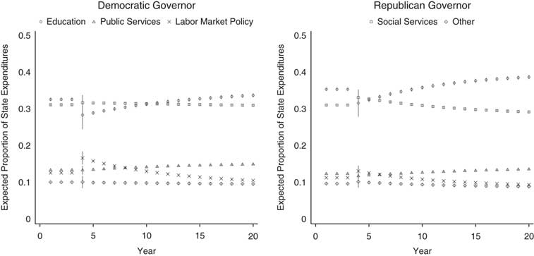
Figure 1 shows an example of a change from baseline simulation from a one standard deviation decrease in personal income at time t=4. The plot on the left shows the starting composition and budgetary response to such a shock under a Democratic governor, while the plot on the right shows the response to the same shock under a Republican governor. Although 95 percent confidence intervals are shown for all time points in the simulation, they are often not much larger than the icons depicting the point estimates with the exception of the shock period at t=4.
Change from baseline dynamic simulation of a one standard deviation decrease to average personal income Note: Starting proportions are set to the sample means under a Democratic and Republican governor for the left and right plots, respectively.

The graphs in Figure 1 allow us to draw a number of substantive conclusions. First, comparing the budgetary starting points for the first three time periods in both graphs, we can see that when all variables are held constant at their means, politics matters. States with a Democratic governor spend slightly more on social services, while states with a Republican governor spend more on education. Differences across the remaining categories are fairly small. When we observe the effects of a decrease in personal income at t=4, there are some similarities and some differences in how budgets change based on the party of the state governor. In both cases, there are substantial drops in the proportion of the budget spent on education and short-run increases in the share for labor market policy. The drop in education is larger for states controlled by a Democratic governor than a Republican one, and in the long-run, Republican governors substantially increase the proportion of the state budget spent on education. In the short-run, the budgetary increase for labor market policy is greater under a Democratic governor than a Republican. In fact, in response to a decrease in average personal income, budgets under a Republican governor do not fluctuate nearly as much as under a Democrat governor.
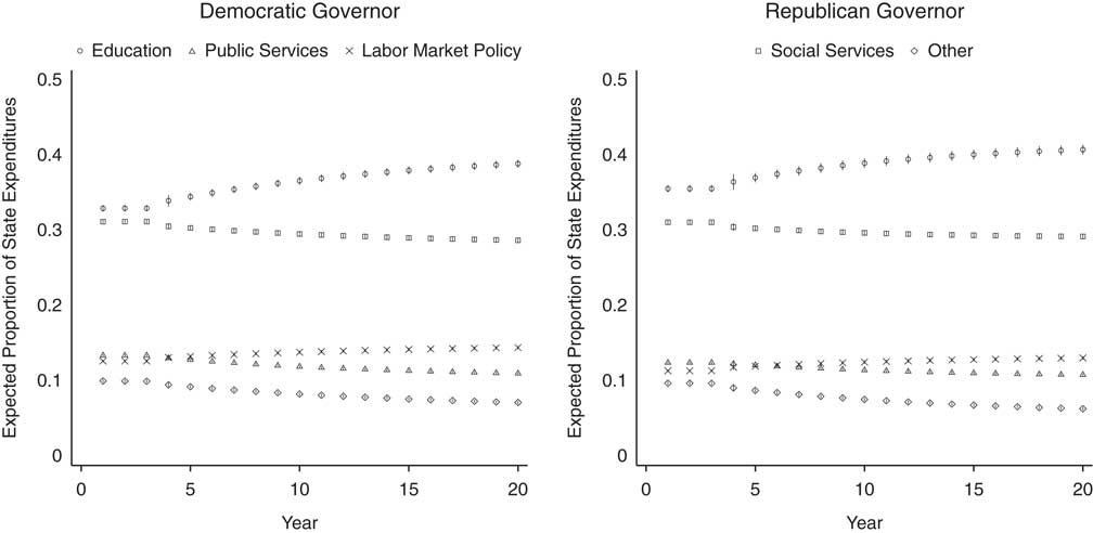
Looking at unemployment, we present the predictions from a change in baseline dynamic simulation for a one standard deviation increase in unemployment in Figure 2. As before, we examine these effects for both a state with a Democratic (left plot) and Republican (right plot) governor. Unlike Figure 1, the responses are largely the same across both parties. In response to an increase in unemployment, both Democratic and Republican governors increase the proportion of the budget going to education, at the cost of social services, public services, and other parts of the budget. Perhaps surprisingly, labor market policy rises only slightly in response to an increase in unemployment.
Change from baseline dynamic simulation of a one standard deviation increase in unemployment

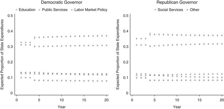
Turning to the spatial effects, we present in Figure 3, the predictions from a change in baseline dynamic simulation for a one standard deviation increase in unemployment in other states, holding all else constant. Here we see much less dramatic budgetary reactions. In both graphs of Figure 3, we see increases in budgets on education and cuts in social services, and surprisingly, the cuts to social services are larger in the Democratic states. In both cases, we also see relative cuts to proportions on the other category and fairly slight cuts to spending on labor market policy and public services. Note too the contrast in the timing of the effects on the budget between internal shocks (Figures 1 and 2) and spatial shocks (Figure 3); spatial shocks tend to have immediate effects, while internal shocks tend to affect the budget much more, but only after a longer period of time.
Change from baseline dynamic simulation of a one standard deviation increase in other states’ unemployment

Change from baseline dynamic simulations like Figures 1 through 3 are helpful for understanding model inferences about the overall trajectories of different parts of a composition over both the short- and long-runs due to a change in the value of a particular independent variable. They represent substantial advancements over previous techniques used to visualize the estimated relationships from models of compositional dependent variables—such as simplex plots—that were limited in the number of dimensions they could present and quite difficult to interpret. However, even dynamic plots can be less than ideal for assessing three simple questions. First, is a particular change statistically significant in the short-run and/or the long-run? Second, is the predicted level of any pair of dependent variable categories overlapping in the short- and long-run? And third, does the relative ordering of the categories change; for example, does a category that was the largest proportion of the budget now become the second largest?
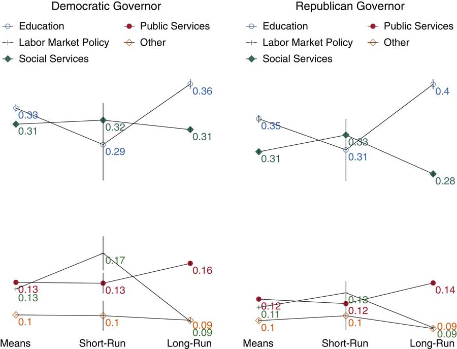
For a cleaner summary of the substantive implications of the results from the change in baseline simulations, we turn to an adaptation of the slope plot (Tufte Reference Tufte1983). In this type of figure, we display expected values for the start of a particular scenario (i.e., the “means” or baseline), the contemporaneous time period in which the simulated shock occurs, and then the long-run level of each category, each with associated confidence intervals. Figure 4 is an example of such a plot for the same income scenario depicted in Figure 1. As with the other figures, estimates for a scenario with a Democratic governor are shown in the left plot and for a Republican in the right. In each plot, the leftmost prediction, labeled “means,” is the expected proportion of each category when all of the independent variables are set to their sample means. The middle prediction in Figure 4, labeled “short-run,” is the expected proportion of each category during the time period in which the one standard deviation decrease in average personal income occurred. The right-most prediction is the long-run expected value for each category that is a new equilibrium level predicted by our model, and the vertical lines running through each prediction depict 95 percent confidence intervals.
Slope plot for a change from baseline dynamic simulation for a one standard deviation decrease to average personal income

Figure 4 allows us to more clearly grasp the estimated changes in the trajectory of the expected value of each category of state budgets. Moreover, the slope plot allows us to see if the relative ordering of the categories has changed over time. Note that in Figure 4, the long-run expected values are different from those at time period 20 in Figure 1, because the trajectories in Figure 1 have not fully adjusted to their new equilibrium values. For example, at time period 20 in the right panel in Figure 1, the budgetary proportion for labor market policy is significantly higher than “Other.” But in the right panel of Figure 4, the long-run proportions for these two categories converges, and they are not significantly different from each other. Overall, Figure 4 helps to show that the three smallest budgetary categories do not end up being very different between Republican and Democratic governors, but education and social services are. In the long-run, in response to a drop in average personal income, Republican governors spend about four percentage points more of their budget on education than Democrats, while Democratic governors spend about two percentage points more of their budget on social services than their Republican counterparts.
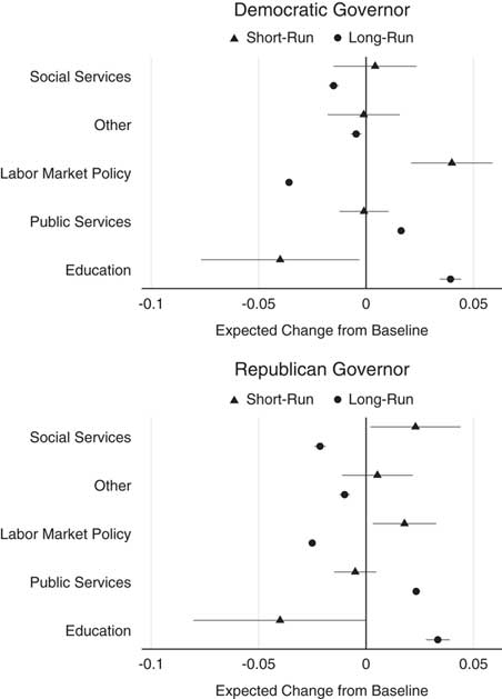
While both the change from baseline plots (e.g., Figure 1) and the slope plots (Figure 4) are useful depictions of the overall predicted trajectory of each category in the same dynamic simulation, it can be complicated to assess whether or not each of the expected short- and long-run changes is significantly different from zero in these types of plots. It is also difficult to discern whether or not these expected changes are different across categories or across the Democratic and Republican scenarios. In order to make these types of assessments, we advocate for the use of an “effects plot” that is similar to the types of coefficient plots that have become popular in recent years. In these plots, we depict both the expected short- and long-run changes to each category due to a change in baseline simulation. Figure 5 is an example of an effects plot for the same scenario of a one standard deviation decrease in average personal income, which we depicted in Figures 1 and 4. In both of the latter figures, it is difficult to determine whether the expected long-run effects are statistically significant for social services. In Figure 5, however, we can now tell that the expected 95 percent confidence intervals for the long-run decrease in social services are statistically significant for both parties, though Republican governors decrease social services by slightly more over the long-run (and they increase it in the short-run). We can also identify that in the short-run, Democratic governors tend to allocate more of their budgets toward labor market policy than Republican governors (and both are statistically significantly different from zero). However, in the long-run, states governed by a Democratic governor tend to decrease the proportion spent on labor market policy—even more so than Republicans—in response to a decrease in average personal income. This figure also makes it clear that, as is often the case with budgeting models, the short-run effects of a particular change tend to be quite modest and not statistically significant, while the long-run effects tend to be quite substantial.
Effect plot for a change from baseline dynamic simulation for a one standard deviation decrease to average personal income

This methodological illustration shows that our suggested strategies for extending the analysis of compositional dependent variables to time series cross-sectional data work well. Although these models produce a large number of parameters, the estimated relationships from them can be easily understood through graphical depictions of post-estimation simulations.
MODELING SPATIALLY LAGGED DEPENDENT VARIABLES
So far, we have shown the utility of compositional time series models with spatially lagged independent variables (spatial-X or SLX models). These specifications test the theoretical proposition that unemployment and personal income in spatially proximate states are likely to have spillover effects on the composition of budgets in other states. However, most models incorporating spatial effects employ a spatially lagged dependent variable (commonly referred to as a SAR). Such models reflect a different type of theoretical proposition where the values of the dependent variable in one state affect the values of the dependent variable in others through diffusion or contagion processes. Using the same example as before, we now specify our model as the following to allow for spatial relationships across values of the dependent variable:
 $$\Delta s_{{ict}} \,{\equals}\,\beta _{{0c}} {\plus}\lambda _{c} {\bf W}\Delta s_{{jct}} {\plus}(1{\plus}d_{{it}} \zeta _{c} )(\Delta x_{{it}} \beta _{c} ){\plus}{\varepsilon}_{{ict}} .$$
Thus, we now have a spatial autoregressive, or SAR model. We take the first-differences of the dependent variable and the two independent variables—unemployment and personal income per capita—and we interact the latter two variables with the partisanship of the governor.Footnote 16 While we assume that ε itc is i.i.d., we estimate Equation 10 using generalized spatial two-stage least squares (Drukker, Prucha and Raciborski Reference Drukker, Prucha and Raciborski2013) that allows us to account for potential heteroskedasticity.Footnote 17
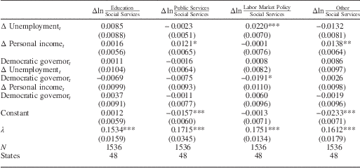
The results of the SAR models are shown in Table 1. The parameter of the spatial lag of the change in logged ratio compositions, λ, is statistically significant across all four models, indicating that spatial dependence is present in the data.
Compositional Spatial Autoregressive Model Results

Note: Generalized spatial two-stage least squares with standard errors in parentheses. Two-tailed tests.
*p<0.10, **p<0.05, ***p<0.01.
EXPLORING THE SUBSTANTIVE IMPLICATIONS OF THE RESULTS
Interpretation of the SAR results in Table 1 is not straightforward, as the coefficients are simultaneously determined with the SAR parameter, λ. As is common with applied spatial econometrics, we use substantively meaningful counterfactual scenarios in order to better understand our results (Ward and Gleditsch Reference Ward and Gleditsch2008). We use two approaches to explore the substantive implications of Table 1. First, we explore how movements in the composition of a given state’s budget affect the budget compositions of spatially proximate states. Second, we explore equilibrium effects of changes in a particular covariate, taking into account the spatial lag.
As shown in Table 1, the parameter on the spatial lag is positive and significant for all four equations. This suggests that, as expected, movements in the budget of one state tend to be associated with similar movements in their spatially proximate neighbors. What would happen to the budgets of other j states, given a budgetary change in state i?Footnote 18 For instance, consider the following scenario. Relative to the previous year, in 2000 Ohio reduced the proportion of expenditures allocated toward education by about 0.5 percentage points. That same year, New Hampshire experienced a large change in education, increasing the share of expenditures by about 11 percentage points. What would the effect be on other states if Ohio would have experienced the same increase as New Hampshire?
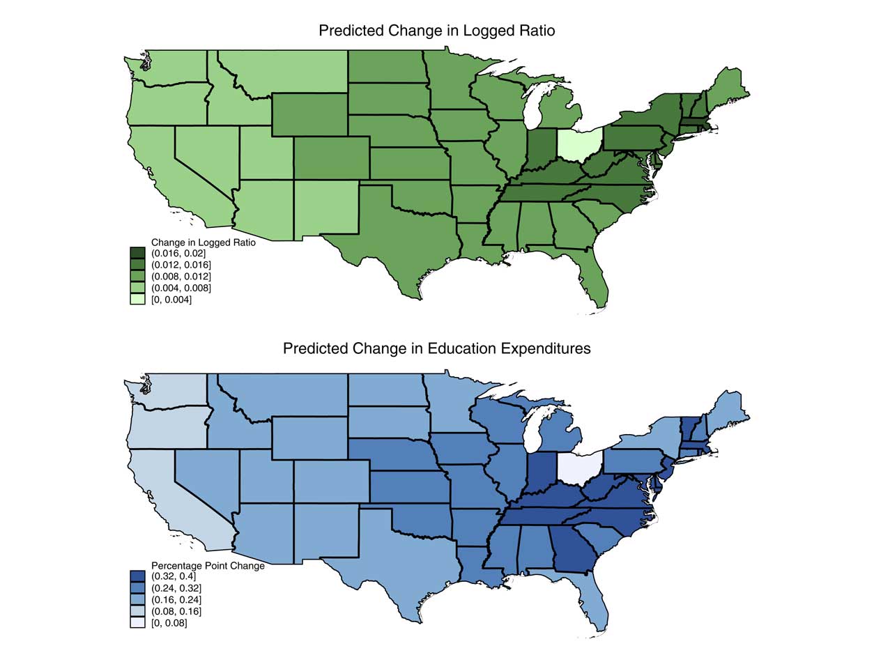
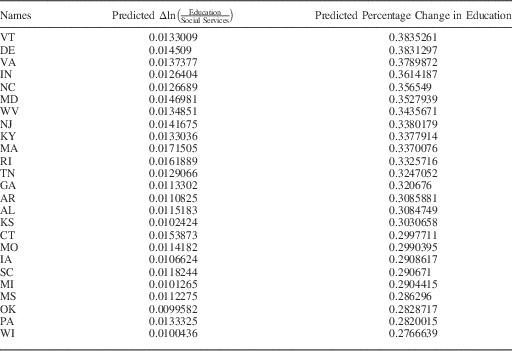
As the dependent variable is compositional, we assume that the 11 percentage point increase to education comes at the expense of all other categories evenly (i.e., 2.75 percentage points).Footnote 19 Given that the dependent variable is a logged ratio between two expenditures, the change in Ohio’s budget needs to be expressed in logged ratio form as well.Footnote 20 We then multiply the spatial weights matrix by a vector of zeros for every state-year except for Ohio in 2000, which experiences the counterfactual change. This is done for each of the four logged ratios. The resulting vectors are then multiplied by the estimated λ for each model, respectively. These vectors show the estimated change in logged-ratio compositions, for each state j, given the increase in education expenditures in state i (Ohio). For instance, the 25 largest predicted changes in the logged ratio of education to social services are shown in the middle column in Table 2. Last, given each predicted change in logged ratio, and the actual values for spending in 1999, we can back out the predicted change in each of the budget categories using the un-transformation formulae given in Equations 8 and 9. The predicted percentage point changes are shown in the right-hand column in Table 2 (see also Figure 6).
Predicted effect of an 11 percentage point increase in Ohio’s education expenditures

Twenty-Five Largest Predicted Changes in Education in Response to an 11 Percentage Point Increase in Ohio’s Education Expenditures

Note: To better visualize these predicted changes, we show both the predicted change in logged ratio (top) and the predicted change in education expenditures (bottom) in Figure 6. As is the case with a logit model, the predicted log-ratio changes are linear, but the predicted percentage changes are not. The size of the predicted percentage changes depends on both the starting value of predicted percentage and the size of the predicted log-ratio change.
SAR REDUCED FORM PREDICTIONS
As a second approach to visualizing the substantive meaning of our results in Table 1, we use reduced form predictions of the impact of simultaneously increasing the personal income in all states by $1000 per capita in the year 2000. We hold the political variable, Democratic governor, constant and calculate reduced form predictions using Table 1 and the actual values of personal income in the year 2000. We then calculate reduced form predictions for the same year but add $1000 to each state’s personal income. As these predictions are still in compositional form, we un-transform them using Equations 8 and 9 and then calculate the difference between the predictions given the counterfactual change and the predictions without that change.
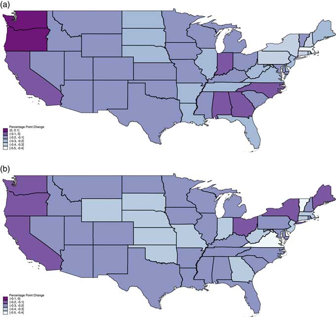
In Figure 7, we present the results for two of the five budgetary categories. As shown in Figure 7a, as a result of a uniform increase of $1000 in personal income across all the states in 2000, all states except for Oregon and Washington spend less on social services, as a percentage of the total budget. Massachusetts is the clear outlier, reducing expenditures by more than 0.4 percent of the total budget. Most other states reduce social services by between 0.1 and 0.3 percentage points, with only a few states (Alabama, California, Georgia, Indiana, North Carolina) decreasing spending by less than 0.1 percentage points. Averaging across all states or calculating the average total impact (ATI) (Drukker, Prucha and Raciborski Reference Drukker, Prucha and Raciborski2013) results in an average decrease of just under one-fifth of 1 percentage point.
The effect of a $1000 increase in personal income in all states in 2000. (a) Change in Social Services (as % of Budget) (b) Change in Education (as % of Budget)

Similar to social services, as shown in Figure 7b, all states also spend relatively less, as a percent of the total budget, on education as a result of a counterfactual increase in personal income. The largest relative decreases are in Vermont and Virginia. The smallest decreases appear to be clustered on the West coast and in the Northeast. The ATI for education is −0.28, meaning that after taking into account spatial effects, the average US state allocates just under one-third of a percentage point less to its education budget, given an increase of $1000 to personal income in states.Footnote 21
CONCLUSIONS AND FUTURE DIRECTIONS
Many important theories in political science and public policy involve compositional dependent variables that vary in interesting ways across time and space. In many cases, however, researchers oversimplify trade-offs to compare just two categories, and they ignore the importance of the effects of time and space. This is especially the case in budgeting, where research has generally focused on trends in one category of spending (i.e., punctuated equilibrium) or the trade-off between two categories (i.e., guns versus butter). In this paper, we have built upon existing approaches, emphasizing dynamic changes to incorporate spatial effects and interactions with contextual variables in time series cross-sectional settings. Through the use of graphical depictions of dynamic simulations, we have shown how our proposed strategy produces a rich set of inferences that can illustrate short- and long-term substantive effects.
In the context of US state expenditures, we have been able to demonstrate how spending trade-offs vary across different governing parties, while also accounting for spillover effects from conditions in other states. While exploring these differences, our approach illustrates how economic shifts, such as a change in income or unemployment can affect relative spending across multiple budgetary categories. Moreover, we find that they also receive different shares of funding from Democrats and Republicans, and that partisanship conditions the effects of economic changes. By incorporating potential spatial effects, we show that not only do surrounding economic conditions affect state budget allocations, but partisanship conditions these effects as well. To assist researchers in the interpretation of their results, we have also adapted a variety of graphical tools for dynamic compositional models.
In future work, there are a number of ways in which our models can be expanded. First, the temporal dynamics of our approach may be extended through vector error correction models that allow us to consider further issues of cointegration. We also are interested in exploring alternative specifications of the spatial weights matrix in order to better model spatial contagion and diffusion from one spatial unit to another. Finally, while we focus this application on the case of state-level budgets, we intend to show the generalizability of our approach to many other political phenomena across multiple countries and policy areas, including political campaigns, issue attention, and income inequality. By advancing our approach and making it accessible to quantitative researchers, we have shown that one can study the space and time characteristics of compositional variables in a broad range of contexts to more closely mirror observed realities.