) plates using the tomographic particle image velocimetry dataset originally obtained by Zhu et al. (2024. J. Fluid Mech.


 plates.

1. Introduction
Flow over an inclined low-aspect-ratio (low- ) plate at low Reynolds numbers is essential in various fluid dynamics applications, such as the design of micro air vehicles (MAVs). A key feature of these flows is the formation of separation bubbles at the critical angle of attack. The complexity of these flows is considerably increased by the interaction of separation bubbles with tip vortices, which arise due to the finite spanwise dimension of the plate. Until now, these complex flows have not been characterised in a comprehensive manner, especially from the perspective of energy exchange. An understanding of energy exchange driven by flow structures and their interactions can provide new insights into flow mechanisms, particularly given the crucial roles that interactions between flow structures play in the development of turbulence. Such insights would be valuable for optimizing flow control and improving the aerodynamic performance of MAVs.
Existing research has concentrated mainly on flow structures and their impact on aerodynamic performance. Typical vortical structures include leading-edge vortices (LEVs) and tip vortices. DeVoria & Mohseni (Reference DeVoria and Mohseni2017) have illustrated that tip vortices induce a downwash, which facilitates a smoother flow at the trailing edge, thereby assisting in the generation of lift at high angles of attack. Moreover, several vortex force approaches have shone additional light on the role of vortical structures on forces, such as the force map method (Li & Wu Reference Li and Wu2018; Li et al. Reference Li, Zhao and Graham2020), the force element/partitioning method (Zhang et al. Reference Zhang, Hayostek, Amitay, He, Theofilis and Taira2020; Menon et al. Reference Menon, Kumar and Mittal2022; Zhu & Breuer Reference Zhu and Breuer2023) and the discrete vortex method (Li et al. Reference Li, Feng, Wang and Liang2023; Kumar et al. Reference Kumar, Padhee and Samanta2024).
The aerodynamic significance of vortices has prompted in-depth investigations into the interactions between vortical structures. Several studies (Taira & Colonius Reference Taira and Colonius2009; Zhang et al. Reference Zhang, Hayostek, Amitay, He, Theofilis and Taira2020; Ribeiro et al. Reference Ribeiro and Taira2022, Reference Ribeiro, Neal, Burtsev, Amitay, Theofilis and Taira2023a
) have demonstrated that tip vortices affect significantly wake stability and forces through interactions with LEVs and other vortices. Furthermore, Tong et al. (Reference Tong, Yang and Wang2020) quantified the competition between LEVs and tip vortices using the vortex-surface method, while Dong et al. (Reference Dong, Choi and Mao2020) statistically characterised the interactions between LEVs and tip vortices. Zhu et al. (Reference Zhu, Wang, Xu, Qu and Long2023, Reference Zhu, Wang and Liu2024) demonstrated that near-wall spanwise flow plays a crucial role in these interactions. In particular, the spanwise flow interplays with the downwash, which determines the transformation patterns of the LEVs. Additionally, triglobal resolvent analysis has been employed to characterise the wake dynamics for low- swept wings (Ribeiro et al. Reference Ribeiro, Yeh and Taira2023b
). Subsequently, the effectiveness of resolvent-analysis-based control was demonstrated (Ribeiro & Taira Reference Ribeiro and Taira2024).
Recently, there has been a growing emphasis on the significance of energy exchange in fluid mechanics, as it can offer valuable insights into vortex dynamics. For instance, it can elucidate the sustaining mechanism of coherent structures (Motoori & Goto Reference Motoori and Goto2021) and the different formation mechanisms between the primary and secondary structures (Baj & Buxton Reference Baj and Buxton2017; Biswas et al. Reference Biswas, Cicolin and Buxton2022). Moreover, energy exchange analysis can provide insight into the nonlinear transfer of kinetic energy, which has significant implications for the modelling of nonlinearity in the Navier–Stokes equations. Recent studies (Jin et al. Reference Jin, Symon and Illingworth2021; Symon et al. Reference Symon, Illingworth and Marusic2021; Wang et al. Reference Wang, Wu and He2025) have highlighted the importance of accurately modelling the nonlinear forcing in order to improve the prediction performance of resolvent analysis. A comprehensive grasp of nonlinear energy transfer can inform the establishment of physical constraints and facilitate advancements in resolvent modelling.
In the study of complex multiscale flows, the decomposition of scales and the derivation of energy budget equations become crucial for energy exchange analysis, and require careful consideration. In the approach based on Reynolds decomposition, a Fourier transform is performed with the objective of decomposing the fluctuating flow field into different wavenumber or frequency patterns. This is done either in the spatial domain (Cho et al. Reference Cho, Hwang and Choi2018; Gomé et al. Reference Gomé, Tuckerman and Barkley2023) or in the temporal domain (Freeman et al. Reference Freeman, Martinuzzi and Hemmati2024; Nekkanti et al. Reference Nekkanti, Colonius and Schmidt2024). Subsequently, the energy exchange between these flow patterns is characterised by the corresponding spectral turbulent kinetic energy (TKE) equations. However, this approach is constrained in its applicability by several issues, including the necessity for periodicity in the spatial domain and the potential for noise pollution in temporal domain analysis. Such noise pollution is particularly evident in experimental studies, as observed in the work of Freeman et al. (Reference Freeman, Martinuzzi and Hemmati2024). As an alternative, triple decomposition offers a promising approach to energy budget analysis. The original triple decomposition proposed by Reynolds & Hussain (Reference Reynolds and Hussain1972) represents the fluctuating flow field as comprising coherent and stochastic parts. It is therefore appropriate to establish energy budgets for the mean, coherent and stochastic motions. It should be noted that random measurement noise is largely included in the stochastic part, thereby mitigating its influence on coherent energy budget analysis. However, this original method considers coherent fluctuations as a whole, thus fails to account for the multiscale flows characterised by multiple simultaneous coherent fluctuations. To address this issue, an extended method is proposed by Baj & Buxton (Reference Baj and Buxton2017). This extended triple decomposition subdivides coherent fluctuations into multiple components, aligning with the existence of multiscale coherent structures in the flows. Additionally, the energy budgets for the coherent motions can be derived in a suitable form accordingly. Subsequently, Kinjangi & Foti (Reference Kinjangi and Foti2023) reformulate the energy budget equations and develop a scale-specific coherent kinetic energy (CKE) evolution methodology that emphasizes triadic interactions and associated energy transfer. The triadic interactions and associated energy transfer arise from the nonlinear terms in the Navier–Stokes equations. The two methods, as proposed by Baj & Buxton (Reference Baj and Buxton2017) and Kinjangi & Foti (Reference Kinjangi and Foti2023), employ optimal mode decomposition (OMD) to distinguish coherent motions. In addition to OMD, alternative techniques are suitable for energy exchange analysis of multiscale flows, including proper orthogonal decomposition (POD; Hosseini et al. Reference Hosseini, Martinuzzi and Noack2016) and spectral POD (Nekkanti et al. Reference Nekkanti, Colonius and Schmidt2024). In flows over low- plates, there exist a variety of length and time scales. The shedding of LEVs occurs at frequencies corresponding to the most amplified perturbations, while subharmonic disturbances become noticeable downstream. Understanding the energy exchanges between these flow motions is crucial for elucidating the development of turbulence. However, the mechanisms of these energy exchanges and their relationship to vortex dynamics remain incompletely understood.
In the present study, we use the same dataset as Zhu et al. (Reference Zhu, Wang and Liu2024), and develop an effective energy budget analysis to quantify the energy exchange. Our primary objective is to enhance our comprehension of the nonlinear inter-scale energy transfer in flows over low- plates. Additionally, we seek to clarify the inherent distinctions between the two identified LEV transformation patterns. The rest of the paper is organized as follows. In § 2, we briefly introduce the dataset used in this study. A coherent energy budget analysis based on the multiscale POD (mPOD) is also developed in this section. Then § 3 discusses the spectral characteristics of the flow fields and the temporal–spatial behaviour of the extracted coherent structures. The budgets for the coherent motions are detailed in § 4, with a focus on nonlinear inter-scale energy transfer. Section 5 delves into the inter-scale interactions that contribute significantly to the energy transfer. Finally, key conclusions are presented in § 6.
2. Methodology
2.1. Dataset description
Plate geometries and coordinate system definition.

The flows on the suction side of four low- plates are investigated experimentally. Figure 1(a) illustrates the planforms of the plates examined in this study, including three rectangular plates and one trapezoidal plate. Each plate has chord length
 $c = {58}\,\textrm {mm}$
and thickness
 $1\, \textrm {mm}$
, with all edges left square. The aspect ratio is defined as the ratio of the maximum span length
 $l_{max}$
to the chord length
 $c$
, denoted as
 . For the three rectangular plates, their respective
 values are
 . For the trapezoidal plate, the
 value is
 $1.38$
with taper angle
 $\beta = 12 ^\circ$
for its side edges. For simplicity, these four plates are referred to as Rect.
 and Trap.
 , respectively. Additional details about the trapezoidal plate can be found in our previous study (Zhu et al. Reference Zhu, Wang, Xu, Qu and Long2023). The natural coordinate system (
 $O$
-
 $xyz$
) is depicted in figure 1(b), where
 $x$
,
 $y$
and
 $z$
represent streamwise, vertical and spanwise coordinates, respectively. The origin
 $O$
is defined so that the midpoint of the trailing edge (indicated by the magenta dot in figure 1
b) is located at
 $(c, 0, 0)$
.
This study utilizes the tomographic particle image velocimetry (PIV) dataset originally obtained by Zhu et al. (Reference Zhu, Wang and Liu2024), which includes the previously unpublished data of the trapezoidal plate. It should be noted that the vortex dynamics observed in the tomographic PIV dataset for the trapezoidal plate is consistent with that elucidated in Zhu et al. (Reference Zhu, Wang, Xu, Qu and Long2023). The freestream velocity is set to
 $U_\infty ={85.8}\, \textrm {mm}\,{\rm s}^{-1}$
, resulting in a chord-based Reynolds number
 ${\textrm{Re}}_c=5400$
. Moreover, the angle of attack is fixed at
 $\alpha = 6 ^\circ$
for all experiments.
In accordance with the strategy adopted by Zhu et al. (Reference Zhu, Wang, Xu, Qu and Long2023, Reference Zhu, Wang and Liu2024), the phase-averaging method is employed in the present study to elucidate the dynamical behaviour of LEVs. The phase information for the LEVs is identified using the POD method, given that the first POD mode pair represents the orthogonal components of the harmonics of the convective LEVs. It should be noted that the fluctuating velocity fields are decomposed within a spatial domain
 $[0.20c, 0.80c]\times [0, 0.22c] \times [-0.30c AR, 0.30c AR]$
. The downstream boundary
 $x/c=0.80$
lies approximately upstream of the appearance of the hairpin vortices, ruling out the hairpin vortex formation process. Once the phase information is determined, the flow fields can be sorted along the phase and averaged using the curve-fitting method (Lengani et al. Reference Lengani, Simoni, Ubaldi and Zunino2014; Toppings & Yarusevych Reference Toppings and Yarusevych2021). This involves the application of an eight-term Fourier model fit to the phase-sorted data at each spatial point individually.
Two representative patterns of the LEV transformations have been revealed by Zhu et al. (Reference Zhu, Wang and Liu2024), presented in figure 2. The spatial morphology of the LEVs is visualized using the orange iso-surfaces
 ${Q^{\theta }c^2}/{U_{\infty }^{2}} = 30$
. In the present study, the
 $Q$
-criterion (Hunt et al. Reference Hunt, Wray and Moin1988; Jeong & Hussain Reference Jeong and Hussain1995) is employed to identify vortical structures and
 $ ( {\cdot } ) ^{\theta }$
denotes a POD-based phase average. For the Rect.
 and
 $1.25$
cases, the LEVs undergo a vortex-splitting transformation as illustrated in figure 2(a). As the phase angle
 $\theta$
increases, the C-shape LEV splits at its head and develops into a -shape vortex. In contrast, a different transformation occurs for the Rect. and Trap.
 cases, whereby the C-shape LEV evolves into an M-shape vortex as shown in figure 2(b). For ease of description, this pattern is hereafter named the vortex-tilting type. Moreover, it has been demonstrated that for all flows studied here, the LEVs interact with the near-wall spanwise flow. The underlying mechanisms of the spanwise fluid transport during the interactions have also been summarized by Zhu et al. (Reference Zhu, Wang and Liu2024), schematized in figure 3. The evolution routine of LEVs is divided into four stages: (i) the development of the separated shear layer; (ii) the convection of C-shape vortices, where the near-wall spanwise flow interacts with the C-shape vortices; (iii) the transformation of C-shape vortices; and (iv) the formation of hairpin vortices. In stage (i), spanwise fluid transport enhances the intensity of the reversed flow, promoting the shear layer roll-up and vortex shedding. In stage (ii), spanwise fluid transport enhances the local upwash on the windward side of the C-shape vortex head, thereby strengthening the vortex head and facilitating the entrainment in the vicinity. In particular, the vortex-splitting transformation occurs in stage (iii) only if the spanwise fluid transport is sufficient to sustain the coherence of LEVs until the vortex head splits in a regular fashion.
Two representative patterns of LEV transformations in flows over low- plates, as reported by Zhu et al. (Reference Zhu, Wang and Liu2024). The vortex-splitting type occurs for the Rect.
 and
 $1.25$
cases, while the vortex-tilting type occurs for the Rect. and Trap.
 cases. The spatial morphology of LEVs is visualized using the
 $Q$
-criterion, with the orange iso-surfaces
 ${Q^{\theta }c^2}/{U_{\infty }^{2}} = 30$
.

Conceptional sketch for the fundamental evolution routine of the vortical structures for low- plates (vortex-splitting type), as revealed by Zhu et al. (Reference Zhu, Wang and Liu2024). The orange and magenta arrows denote two mechanisms associated with the near-wall spanwise flow.

In the present study, an energy budget analysis is performed to shed new light on the nonlinear energy exchanges involved in the two types of LEV transformations. The data are acquired at sampling frequency
 $f_s= 216\,\textrm {Hz}$
. They consist of
 $7265$
snapshots, spanning approximately
 $110$
vortex-shedding cycles. The vector resolution in the velocity fields is
 $0.56\,\textrm {mm}$
(
 $0.01c$
). All raw data are validated and smoothed using the robust divergence-free smoothing algorithm (Wang et al. Reference Wang, Gao, Wang, Wei, Li and Wang2016) and the Savitzky–Golay filter, in accordance with the procedures adopted by Zhu et al. (Reference Zhu, Wang and Liu2024). Focusing on the LEV evolution, the energy budget analysis is performed within a spatial domain
 $\Omega$
:
 $[0.25c, 1.00c]\times [0, 0.22c] \times [-0.30c AR, 0.30c AR]$
. It should be noted that the variable spanwise dimension has a negligible impact on the present analysis, as the positioning of the spanwise boundary ensures that velocity fluctuations in its vicinity are insignificant. Due to the spatial resolution and the noise levels of the current tomographic PIV measurements, it is difficult to resolve the kinetic energy budgets for stochastic fluctuations. Nevertheless, as our main objective is to study the nonlinear energy exchanges resulting from LEV dynamics, only CKE budgets are considered in this study. For further details on the dataset and experimental methodology, refer to Zhu et al. (Reference Zhu, Wang and Liu2024).
2.2. The mPOD method and triple decomposition
This section introduces the mPOD method, which is employed to distinguish the coherent motions from the mean flow and stochastic fluctuations.
The mPOD method, proposed by Mendez et al. (Reference Mendez, Balabane and Buchlin2019), utilizes a user-defined frequency splitting vector to partition the correlation matrix of the dataset into contribution of multiple scales. These scales retain non-overlapping portions of the frequency spectra. Subsequently, standard POD is performed independently at each scale. The result of this decomposition can be expressed as
 \begin{equation} \boldsymbol {u}(\boldsymbol {x},t) = \overline {\boldsymbol {u}}(\boldsymbol {x}) + \sum \limits _{l,r} {a^{[l,r]}(t)\, \boldsymbol {\phi }^{[l,r]}(\boldsymbol {x})}, \end{equation}
where
 $\overline {\boldsymbol {u}}(\boldsymbol {x})$
is the (time-averaged) mean velocity field, and
 $a^{[l,r]}(t)$
denotes the temporal coefficient corresponding to the
 $r$
th mPOD mode
 $\boldsymbol {\phi }^{[l,r]}(\boldsymbol {x})$
at the
 $l$
th scale. Orthonormal rules are maintained between different mPOD modes:
 \begin{equation} \left . \begin{array}{l} \displaystyle \overline {a^{[l,r]} \, a^{[m,k]} } = \delta _{lm} \delta _{rk} \lambda ^{[l,r]}, \\[3pt] \displaystyle \boldsymbol {\phi }^{[l,r]}\boldsymbol {\cdot } \boldsymbol {\phi }^{[l,k]} =\delta _{rk}. \end{array} \right \} \end{equation}
Here,
 $\lambda ^{[l,r]}$
is the eigenvalue measuring the energy contained in the corresponding mPOD mode, and
 $\delta _{ij}$
is the Kronecker delta function.
The triple decomposition is then achieved by designating the first two most energetic mPOD modes as the coherent part for the
 $l$
th scale
 $\tilde {\boldsymbol {u}}^l (\boldsymbol {x},t)$
. This number of modes is selected because when the
 $l$
th scale is dominated by a convective structure, the first two mPOD modes at this scale should occur in a pair. This mode pair represents the orthogonal components of the harmonics of the convective structure (Oudheusden et al. Reference van Oudheusden, Scarano, van Hinsberg and Watt2005; Lengani et al. Reference Lengani, Simoni, Ubaldi and Zunino2014). The triple decomposition of multiscale flows can be formulated as
 \begin{eqnarray} \begin{aligned} \boldsymbol {u}\left ( \boldsymbol {x},t \right ) &= \hspace {0.35em} \overline {\boldsymbol {u}}\left ( \boldsymbol {x} \right ) \hspace {0.35em} + \hspace {0.35em} \sum _l{\boldsymbol {\tilde {u}}^l\left ( \boldsymbol {x},t \right )} \hspace {0.35em} + \hspace {0.35em} \boldsymbol {u}^{\prime \prime }\left ( \boldsymbol {x},t \right )\\ &= \underbrace {\vphantom {\sum \limits _{r=1}} \hspace {0.1em} \overline {\boldsymbol {u}}\left ( \boldsymbol {x} \right ) \hspace {0.1em} }_{ \text {Mean part}} + \hspace {0.35em}\sum _l{{\underbrace {\sum _{r=1}^2{a^{\left [ l,r \right ]}\left ( t \right ) \boldsymbol {\phi }^{\left [ l,r \right ]}\left ( \boldsymbol {x} \right )}}_{\text {Coherent part for $l$th scale}}}} \hspace {0.35em}+ {\underbrace {\vphantom {\sum \limits _{r=1}} \hspace {0.1em} \boldsymbol {u}^{\prime \prime }\left ( \boldsymbol {x},t \right ) \hspace {0.1em} }_{\text {Stochastic part}}}.\\ \end{aligned} \end{eqnarray}
Here,
 $\boldsymbol {u}^{\prime \prime }(\boldsymbol {x},t)$
corresponds to stochastic fluctuations.
In comparison to alternative flow decomposition techniques, mPOD demonstrates significant capabilities in the identification of coherent structures and the triple decomposition of multiscale flows. First, in contrast to OMD, mPOD is not constrained by the linear dynamical approximation, thus enabling the direct extraction of coherent structures with a nonlinear nature, such as the secondary structures energized by nonlinear triadic interactions. The extraction of such secondary structures has previously necessitated the utilisation of supplemental techniques (Baj & Buxton Reference Baj and Buxton2017; Biswas et al. Reference Biswas, Cicolin and Buxton2022). In addition, mPOD is capable of fully identifying coherent structures by allowing them to act within specific frequency bands. As demonstrated by Mendez et al. (Reference Mendez, Balabane and Buchlin2019), this feature results in better convergence compared to harmonic decompositions such as dynamic mode decomposition (DMD). Finally, owing to its modal orthogonality, mPOD is a viable technique for triple decomposition of multiscale flows, as demonstrated by Roudnitzky et al. (Reference Roudnitzky, Druault and Guibert2006) for the case of POD. These strengths of mPOD promote the derivation of corresponding energy budget equations, as proposed in the next subsection.
2.3. The CKE budget
After achieving the triple decomposition, the kinetic energy budget can be derived based on the incompressible Navier–Stokes equations. Following an approach similar to that proposed by Baj & Buxton (Reference Baj and Buxton2017), the CKE budget equation at the
 $l$
th scale can be derived as follows, using Einstein’s summation convention:
 \begin{align} &\underbrace { \vphantom {\sum \limits _{m,n}} \frac {\partial \tilde {k}^l}{\partial t }}_{\widetilde {\mathcal {L}}^l} + \underbrace { \vphantom {\sum \limits _{m,n}}\overline {u}_j \frac {\partial \tilde {k}^l}{\partial x_j}}_{\widetilde {\mathcal {C}}^l} = \underbrace { \vphantom {\sum \limits _{m,n}} -\overline {\tilde {u}_i^l\tilde {u}_j^l}{\frac {\partial \overline {u}_{i}}{\partial x_j}}}_{\widetilde {\mathcal {P}}^l} -\underbrace { \vphantom {\sum \limits _{m,n}} \left(-\overline {u_i^{\prime\prime} u_j^{\prime\prime} \frac {\partial \tilde{u}_{i}^l}{\partial x_j} }\right)}_{\widehat {\mathcal {P}}^l} + \underbrace { \sum \limits _{m,n}{\frac {1}{2}}\left(\overline {\tilde {u}_i^n\tilde {u}_j^m\frac {\partial \tilde {u}_i^l}{\partial x_j}} - \overline {\tilde {u}_i^l\tilde {u}_j^m\frac {\partial \tilde {u}_i^n}{\partial x_j}}\right)}_{\widetilde {\mathcal {T}}^l} \nonumber \\ &\quad - \underbrace { \vphantom {\sum \limits _{m,n}} 2\,{{\textrm{Re}}}^{-1}\,\overline {\tilde {s}_{ij}^l\tilde {s}_{ij}^l}}_{\widetilde {\epsilon }^l} + \underbrace { \frac {\partial }{\partial x_j}\left(-\overline {\tilde {u}_j^l{\tilde {p}^l}} - \sum \limits _{m,n}{\frac {1}{2}}\overline {\tilde {u}_i^l\tilde {u}_j^m\tilde {u}_i^n} - \overline {u_i^{\prime \prime } u_j^{\prime \prime } \tilde {u}_i^l} + 2\,{{\textrm{Re}}}^{-1}\,\overline {\tilde {u}_i^l\tilde {s}_{ij}^l}\right) }_{\widetilde {\mathcal {D}}^l}. \end{align}
Here,
 $u_i$
is the
 $i$
th component of the velocity
 $\boldsymbol {u}$
,
 $\tilde {k}^l = (1/2)\overline {\tilde {u}_i^l\tilde {u}_i^l}$
is the CKE, and
 $\tilde {s}_{ij}^l = (1/2)({\partial \tilde {u}_{i}^l}/{\partial x_j} + {\partial \tilde {u}_{j}^l}/{\partial x_i})$
is the strain rate.
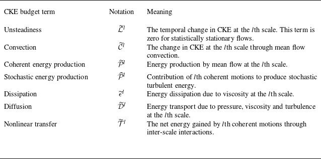
The left-hand side of (2.4) represents the change in CKE at the
 $l$
th scale due to local unsteadiness
 $\widetilde {\mathcal {L}}^l$
and convection
 $\widetilde {\mathcal {C}}^l$
. In the case of statistical stationary flows, the term
 $\widetilde {\mathcal {L}}^l$
goes to zero. The right-hand side represents the cause of the change. Specifically, the terms
 $\widetilde {\mathcal {P}}^l$
and
 $\widehat {\mathcal {P}}^l$
denote the production of CKE and stochastic turbulent energy at the
 $l$
th scale, respectively. The term
 $\widetilde {\mathcal {\epsilon }}^l$
represents the direct dissipation, while the term
 $\widetilde {\mathcal {D}}^l$
accounts for the diffusive energy transport due to pressure, viscosity and turbulence. The nonlinear energy transfer term
 $\widetilde {\mathcal {T}}^l$
quantifies the net CKE gained by the
 $l$
th coherent motion through inter-scale interactions. All terms of the CKE budget equation at the
 $l$
th scale are featured explicitly in table 1.
Terms of the CKE budget at the
 $l$
th scale.

The finite bandwidth of mPOD modes serves to enhance the feasibility of the proposed CKE budget analysis for complex flows. It is evident that in certain flows, the existing methods based on harmonic decomposition (e.g. DMD and spectral POD) are adequate for energy budget analysis (Jin et al. Reference Jin, Symon and Illingworth2021; Biswas et al. Reference Biswas, Cicolin and Buxton2022; Nekkanti et al. Reference Nekkanti, Colonius and Schmidt2024). This can be attributed to the narrow bandwidth of the spectral peaks representing each scale, with these peaks being widely spaced in the spectrum. It can thus be surmised that the impact of other frequency components within each narrow bandwidth is likely to be insignificant in this context. However, for transitional and turbulent flows in general, the bandwidth of peaks may be broad, with other components also contributing to the energy budget. In this scenario, methods that constrain a single harmonic at each scale may underestimate coherent energy, potentially introducing inaccuracies in the CKE budget. Therefore, it is preferable to associate coherent motions with a frequency band rather than a single frequency for CKE budget analysis. This principle is imposed inherently in mPOD, making it suitable for CKE budget analysis.
The determination of scales is crucial for the mPOD-based CKE budget analysis. In this study, a scale refers to a specific frequency band within which the motions occurring are characterised by consistent flow physics. For instance, the roll-up of the shear layer and subsequent vortex shedding commonly manifest as a broad spectral peak in the spectrum (Yarusevych et al. Reference Yarusevych, Sullivan and Kawall2009; McAuliffe & Yaras Reference McAuliffe and Yaras2010). Accordingly, the broad frequency band is identified as a single scale. Furthermore, the definition of scales adopted here aligns with that in multi-resolution analysis.
2.4. Scale triads and their relation to triadic interaction
The significant role of triadic interactions in inter-scale energy transfer has been widely acknowledged in the literature (Baj & Buxton Reference Baj and Buxton2017; Kinjangi & Foti Reference Kinjangi and Foti2023; Nekkanti et al. Reference Nekkanti, Nidhan, Schmidt and Sarkar2023, Reference Nekkanti, Colonius and Schmidt2024; Freeman et al. Reference Freeman, Martinuzzi and Hemmati2024). This subsection provides a definition of scale triads and distinguishes them from the familiar frequency triads. It then proceeds to establish a connection between inter-scale energy transfer through scale triads and triadic interactions.
Sketches of (a) the scale partitioning paradigm, (b) regions of the bispectrum, and (c) segmentation of the bispectrum by scale triads. Non-negative by definition, the frequencies
 $f_n$
and
 $f_m$
reside on the frequency axes
 $ f^n$
and
 $f^m$
.

Figure 4(a) illustrates the scale partitioning paradigm that is employed in the present study. The coloured boxes on the frequency axis represent the scales, with equal bandwidth and spacing. The proposed paradigm is characterised by the positioning of frequency
 $f = 0$
at the centre of the scale (i.e. the pink-coloured box), while allowing for the customisation of bandwidth and number of scales. This paradigm provides advantages in analysing inter-scale interactions, as will be demonstrated below. Alternative scale partitioning paradigms may also be suitable for other applications.
Figure 4(b) depicts the representative bispectrum, a commonly employed visualisation technique for triadic interactions (Kim & Powers Reference Kim and Powers1979; Lii & Helland Reference Lii and Helland1981). The large hexagonal region is constrained by the sampling frequency
 $f_s$
. A triadic interaction is said to occur when the frequencies (e.g.
 $f_l$
,
 $f_m$
and
 $f_n$
) satisfy the zero-sum condition, which is expressed as
 $f_n \pm f_m \pm f_l = 0$
. In other words, these frequencies form a frequency triad, representing a point in the bispectrum. The triadic interactions consist of the sum-interactions (
 $f_l = f_n + f_m$
) and the difference-interactions (
 $f_l = f_n - f_m$
). The former correspond to the principal region in figure 4(b), while the latter correspond to the conjugate region. The remaining grey regions contain only redundant information due to the symmetry of the bispectrum. Thus the frequency triad can be expressed as
 $(f_n,f_m,f_l)$
or
 $(f_n,f_m)$
, given that
 $f_l$
can be derived from the other frequencies,
 $f_l = f_n \pm f_m$
. On the other hand, inter-scale interaction occurs when the frequencies within the three individual scales (e.g.
 $l$
th,
 $m$
th and
 $n$
th scales) form triads. As with the definition of frequency triads, these scales can be combined as a scale triad, represented as
 $( n | m | l)$
. It should be noted that the zero-sum condition applies to frequency triads but not to scale triads, such that
 $l$
is not redundant for scale triads. A representative scale triad in the bispectrum is illustrated by the orange hexagon in figure 4(b).
In consideration of scale partitioning, the bispectrum can be segmented into a number of regions, each corresponding to a specific scale triad. Figure 4(c) illustrates the outcomes of this segmentation. The hexagons and triangles, delineated by dotted lines, represent scale triads. In particular, a scale triad of the hexagonal type occurs when the central frequencies of the three individual scales align to form a frequency triad. The scale partitioning paradigm proposed in figure 4(a) ensures that these scale triads uniformly and regularly segment the bispectrum without any overlap or gap. Consequently, nonlinear interactions can now be examined in a hierarchical manner. This novel hierarchical framework elucidates the inter-scale interactions, while allowing for further exploration of the underlying triadic interactions of interest. Furthermore, the integration in the frequency domain enhances robustness against measurement noise. Overall, it is of value to introduce the concept of scale triads and the corresponding hierarchical framework for studying complex flows.
The hierarchical framework based on scale triads can be further leveraged to explore the nonlinear energy transfer. To achieve this, the term
 $\widetilde {\mathcal {T}}^l$
is first expanded to the sum of energy transferred by scale triads:
 \begin{equation} \widetilde {\mathcal {T}}^l=\sum _{m,n}{\widetilde {\mathcal {T}}\left ( n | m | l\right )}, \end{equation}
with
 \begin{equation} \widetilde {\mathcal {T}}\left ( n | m | l\right )=\frac {1}{2}\left(\overline {\tilde {u}_i^n\tilde {u}_j^m \frac {\partial \tilde {u}_i^l}{\partial x_j}}-\overline {\tilde {u}_i^l\tilde {u}_j^m \frac {\partial \tilde {u}_i^n}{\partial x_j}}\right). \end{equation}
In particular, the specific inter-scale energy transfer term
 $\widetilde {\mathcal {T}}( n | m | l)$
represents the net CKE transfer through a pathway from the
 $n$
th scale (giver) to the
 $l$
th scale (receiver), with the
 $m$
th scale acting as a mediator (Smyth Reference Smyth1992).
A bispectrum analysis is then conducted to explore the triadic couplings underlying inter-scale energy transfer. The term
 $\widetilde {\mathcal {T}}( n | m | l)$
is decomposed into temporal and spatial components:
 \begin{equation} \widetilde {\mathcal {T}}\left ( n | m | l\right ) =\sum _{r_n=1}^2{\sum _{r_m=1}^2{\sum _{r_l=1}^2{ \frac {1}{2} \boldsymbol {A}^{\left ( r_n,r_m,r_l \right )}_{\left ( n \left | m \right | l\right )} \boldsymbol {\Phi }^{\left ( r_n,r_m,r_l \right )}_{\left ( n \left | m \right | l\right )} }}}, \end{equation}
with
 \begin{equation} \left . \begin{array}{l} \begin{aligned} \displaystyle \boldsymbol {A}^{\left ( r_n,r_m,r_l \right )}_{\left ( n \left | m \right | l\right )} & = \overline {a^{\left [ l,r_l \right ]}a^{\left [ m,r_m \right ]}a^{\left [ n,r_n \right ]}}, \\[3pt] \displaystyle \boldsymbol {\Phi }^{\left ( r_n,r_m,r_l \right )}_{\left ( n \left | m \right | l\right )} & = \left ( \phi _{i}^{\left [ n,r_n \right ]}\phi _{j}^{\left [ m,r_m \right ]}\frac {\partial \phi _{i}^{\left [ l,r_l \right ]}}{\partial x_j}-\phi _{i}^{\left [ l,r_l \right ]}\phi _{j}^{\left [ m,r_m \right ]}\frac {\partial \phi _{i}^{\left [ n,r_n \right ]}}{\partial x_j} \right ). \end{aligned} \end{array} \right \} \end{equation}
Here,
 $r_l$
,
 $r_m$
and
 $r_n$
denote the orders of mPOD modes at the
 $l$
th,
 $m$
th and
 $n$
th scales, respectively. Meanwhile,
 $\phi _{i}^{[ l,r_l ]}$
represents the
 $i$
th component of the
 $r_l$
th mPOD mode at the
 $l$
th scale
 $\boldsymbol {\phi }^{[ l,r_l ]}$
. The temporal behaviour of specific inter-scale energy transfer is exclusively characterised by
 $\boldsymbol {A}^{( r_n,r_m,r_l )}_{( n | m | l)}$
. A Fourier decomposition of the temporal coefficients gives
 \begin{equation} a^{[l,r]}(t) = \sum \limits _{f_l = -\infty }^{\infty }{\hat {a}^{[l,r]}(f_l) \exp {(j 2{\unicode[Arial]{x03C0}} f_l t)}}, \end{equation}
with
 $j = \sqrt {-1}$
. Then inserting (2.9) into
 $\boldsymbol {A}^{( r_n,r_m,r_l )}_{( n | m | l)}$
yields
 \begin{equation} \boldsymbol {A}^{\left ( r_n,r_m,r_l \right )}_{\left ( n \left | m \right | l\right )} = \sum \limits _{f_n = -\infty }^{\infty } {\sum \limits _{f_m = -\infty }^{\infty } {\sum \limits _{f_l = -\infty }^{\infty }{ \widehat {\boldsymbol {A}}^{\left ( r_n,r_m,r_l \right )}_{\left ( n \left | m \right | l\right )}\, \overline {\exp {[ j 2{\unicode[Arial]{x03C0}} (f_n+f_m+f_l) t ]}} }}}, \end{equation}
with
 $\widehat {\boldsymbol {A}}^{( r_n,r_m,r_l )}_{( n | m | l)}=\hat {a}^{[n,r_n]}(f_n)\, \hat {a}^{[m,r_m]}(f_m)\, \hat {a}^{[l,r_l]}(f_l)$
. Importantly, the triadic interactions are imposed by (2.10) as
 $\boldsymbol {A}^{( r_n,r_m,r_l )}_{( n | m | l)}$
is non-zero only when the frequencies form a triad. Together with the symmetry of the bispectrum,
 $\boldsymbol {A}^{( r_n,r_m,r_l )}_{( n | m | l)}$
can be formulated as
 \begin{align} \boldsymbol {A}^{\left ( r_n,r_m,r_l \right )}_{\left ( n \left | m \right | l\right )} & =\sum \limits _{f_n=0}^{\infty }{\sum \limits _{f_m=-\infty }^{\infty }{ 2 \textrm{Re} { \{\hat {a}^{[n,r_n]}(f_n)\, \hat {a}^{[m,r_m]}(f_m)\, \hat {a}^{[l,r_l]\ast }(f_n+f_m) \} } }} \nonumber\\ & =\sum \limits _{f_n=0}^{\infty }{\sum \limits _{f_m=-\infty }^{\infty }{ 2{\textrm{Re}} { \{ \widehat {\boldsymbol {A}}^{\left ( r_n,r_m,r_l \right )}_{\left ( n \left | m \right | l\right )}(f_n,f_m) \} } }}, \end{align}
where the superscript
 $^\ast$
stands for conjugate transpose, and
 ${\textrm{Re}} {\{{\cdot }\}}$
denotes the real part of a complex quantity. Finally, the specific inter-scale energy transfer term
 $\widetilde {\mathcal {T}}( n | m | l)$
is expanded to the sum of energy transferred by triadic interactions:
 \begin{equation} \widetilde {\mathcal {T}}\left ( n \left | m \right | l\right ) = \sum \limits _{f_n=0}^{\infty }{\sum \limits _{f_m=-\infty }^{\infty }{ \widetilde {\mathcal {T}}^{\left ( n \left | m \right | l\right )}(f_n,f_m) }}, \end{equation}
with
 \begin{equation} \widetilde {\mathcal {T}}^{\left ( n \left | m \right | l\right )}(f_n,f_m) = \sum _{r_n=1}^2{\sum _{r_m=1}^2{\sum _{r_l=1}^2{ {\textrm{Re}} { \{ \widehat {\boldsymbol {A}}^{\left ( r_n,r_m,r_l \right )}_{\left ( n \left | m \right | l\right )}(f_n,f_m) \}} \boldsymbol {\Phi }^{\left ( r_n,r_m,r_l \right )}_{\left ( n \left | m \right | l\right )} }}}. \end{equation}
Given that
 $f_n$
and
 $f_m$
can refer to
 $n$
th and
 $m$
th scales, respectively,
 $\widetilde {\mathcal {T}}^{( n | m | l)}(f_n,f_m)$
is abbreviated as
 $\widetilde {\mathcal {T}}^{l}(f_n,f_m)$
hereinafter for notational simplicity.
3. Extraction of multiscale coherent structures
Volume-integral power spectral density for all investigated cases.

We start by examining the global spectral characteristics of the flow fields. Figure 5 presents the volume-integral power spectral density (
 $\textit {PSD}$
) as a function of the Strouhal number
 $St\equiv f c \sin \alpha /U_\infty$
. For each case, the integration is performed along the three velocity components at every spatial location within the spatial domain
 $\Omega$
, which is defined in § 2.1 and utilized in the CKE budget analysis. The
 $\textit {PSD}$
value is estimated using the Thomson’s multi-taper method (Thomson Reference Thomson1982) with two sine tapers and
 $7265$
points. The number of tapers adopted has a minimal impact on the flow physics under consideration, as evidenced in Appendix A. The resulting frequency resolution is
 $St = 0.002$
. A distinct peak at
 $St_1 = 0.238$
can be observed in each spectrum, reflecting the time scale of one LEV formation-shedding event.
By comparing the energy distributions of the subharmonic components near
 $0.5\,St_1$
, valuable insights can be gained. In cases with Rect. and Trap.
 , the energy is predominantly concentrated at
 $0.5\,St_1$
. This indicates that the effective triadic interaction may involve only the
 $0.5\,St_1$
and
 $St_1$
components. In contrast, for the Rect.
 and
 $1.25$
cases, additional spectral peaks emerge at approximately
 $0.5\,St_1$
, specifically at frequencies
 $0.46\,St_1$
and
 $0.53\,St_1$
for the Rect.
 case, and at frequencies
 $0.41\,St_1$
and
 $0.58\,St_1$
for the Rect.
 case. The sum of each frequency pair closely approximates
 $St_1$
, suggesting that multiple triads may take a role in the nonlinear interactions between the fundamental vortex-shedding motion and the corresponding subharmonic motions. Additionally, a discernible peak appears at
 $St = 0.192$
(
 $0.82\,St_1$
) for the Rect.
 and
 $1.25$
cases. Both peaks at
 $0.82\,St_1$
and
 $St_1$
exhibit consistent flow physics, namely the development of LEVs (see Appendix B for details). It is of particular significance that the different spectral energy distributions observed at the subharmonics align with the two LEV transformation patterns (as demonstrated in figure 2). This suggests a potential correlation between the active nonlinear interactions and the LEV dynamics.
This fundamental frequency
 $St_1$
is then used to define the frequency splitting vector as
 $F_V = [0.25\,St_1, 0.75\,St_1, \ldots , 2.25\,St_1]$
, with resulting scales distinguished by line colours in figure 5. For simplicity, the notation
 $\langle \text {central frequency of a band} / St_1\rangle$
is used to represent these scales. For example, the fundamental scale
 $[0.75\,St_1, 1.25\,St_1]$
is expressed as
 $\langle 1.0\rangle$
. In particular, the scale
 $[0, 0.25\,St_1]$
is denoted by
 $\langle \varDelta \rangle$
as it characterises the slowly varying component in the flows. It is noteworthy that the selected bandwidth prevents the unnecessary attenuation of the characteristic frequency components of interest within the filtered signal during the mPOD process, thereby ensuring the completeness of the extracted coherent structures. Additionally, the scale partitioning is optimal for the present study as the focus is placed on the fundamental scale and its half-harmonic scale. It is acknowledged that if the primary focus is directed towards other triadic interactions, then the scale can be partitioned in alternative ways to analyse the flow structures and the associated energy exchange accordingly.
Relative energy distributions of the first ten mPOD modes at different scales for all investigated cases. The percentages in the second and third columns indicate the contributions of coherent motions to the total TKE at the corresponding scales.

The
 $\textit {PSD}$
of the normalized temporal coefficients of the mPOD modes at the
 $\langle 0.5\rangle$
and
 $\langle 1.0\rangle$
scales. The vertical grey lines represent the frequency splitting vector. The upper insets illustrate the energy distributions of the coherent motions at the
 $\langle 1.0\rangle$
scale, given by the orange iso-surfaces
 $\textit {CKE}^{\langle 1.0\rangle } = 2.4\times 10^{-5}$
.

Next, the mPOD analysis is performed to extract the coherent structures. Given that the contained energy is negligible, and no distinct peak is observed for
 $St \gt 2.25\,St_1$
, no coherent structure is extracted from this portion. Figure 6 presents the relative energy distributions of the first ten modes at each individual scale, with red dots representing the coherent modes. Notably, the first two modes contain almost identical energy for both the
 $\langle 0.5\rangle$
and
 $\langle 1.0\rangle$
scales, with their spatial distributions at each scale being similar (not shown here for brevity). These distinct features imply that these modes occur in pairs, representing convective coherent structures (Oudheusden et al. Reference van Oudheusden, Scarano, van Hinsberg and Watt2005; Lengani et al. Reference Lengani, Simoni, Ubaldi and Zunino2014). Moreover, the coherent structures at these two scales contribute to at least
 $40\,\%$
of the total TKE, underscoring their dominance of the flows.
The focus now turns towards examining the dynamics of coherent motions at
 $\langle 0.5\rangle$
and
 $\langle 1.0\rangle$
scales. Figure 7 presents the
 $\textit {PSD}$
of normalized modal coefficient
 $a^{[l,r]}/\sqrt {\lambda ^{[l,r]}}$
. It is noteworthy that the peaks identified from modal
 $\textit {PSD}$
agree with those identified from the volume-integral
 $\textit {PSD}$
(in figure 5). This agreement demonstrates the manifestation of global dynamical behaviour in the identified coherent structures within the flows.
Further insights can be gained by comparing the energy distributions of the coherent motions. To achieve this, the normalized CKE at the
 $l$
th scale is defined by
 \begin{equation} \textit {CKE}^{l}(\boldsymbol {x}) = \frac {\sum _{r=1,2}{\lambda ^{[l,r]}\, \phi _i^{[l,r]}(\boldsymbol {x})\, \phi _i^{[l,r]}(\boldsymbol {x})}} {\sum _{r=1,2}{\lambda ^{[l,r]}}}. \end{equation}
In the upper inset of figure 7, the energy distributions are depicted by the orange iso-surfaces
 $\textit {CKE}^{\langle 1.0\rangle } = 2.4\times 10^{-5}$
. Note that only the energy distribution at the
 $\langle 1.0\rangle$
scale is compared, given that no significant disparity is observed for the other scales. While the
 $\textit {CKE}^{\langle 1.0\rangle }$
distribution remains analogous across all cases, a notable exception is evident near the midspan. A distinct tail structure emerges for the Rect. and Trap.
 cases, as indicated by the blue dashed box. Remarkably, the most pronounced discrepancy between the two LEV transformations also occurs near the midspan. This is evidenced by the evolution of the head portion of the C-shape LEVs, as illustrated in figure 2. The spatial consistency suggests that the LEV transformations are associated with coherent motion at the fundamental scale.
4. Coherent energy budget analysis
Having inspected the coherent motions at different scales, we proceed to examine the overall energy balance among the coherent motions, with a specific focus on inter-scale energy transfer.
Terms of the coherent energy budget. The CKE budget terms are denoted by the generic variable
 $E$
. Values are expressed as percentages of the total coherent energy productions
 $\sum \nolimits _l{\widetilde {\mathcal {P}}^l}$
.

Net contribution of nonlinear energy transfer terms
 $\widetilde {\mathcal {T}}^l$
. Values are expressed as percentages of the total coherent energy productions
 $\sum \nolimits _l{\widetilde {\mathcal {P}}^l}$
.

The relative contributions of the coherent energy terms at each scale are given in figure 8. The pressure component appearing in the diffusion term
 $\widetilde {\mathcal {D}}^l$
cannot be accessed directly and is therefore estimated from the residuals of other terms. In all cases examined in this study, the coherent motions are energized primarily by the mean flow at
 $\langle 0.5\rangle$
and
 $\langle 1.0\rangle$
scales, via the coherent energy production term
 $\widetilde {\mathcal {P}}^l$
. Furthermore, it appears that the energy gained by
 $\widetilde {\mathcal {P}}^l$
is predominantly balanced by convection
 $\widetilde {\mathcal {C}}^l$
and diffusion
 $\widetilde {\mathcal {D}}^l$
. The large term
 $\widetilde {\mathcal {C}}^l$
is associated with the downstream evolution of LEVs, which carry energy away from the integration domain
 $\Omega$
through its downstream boundary. This phenomenon has a minimal impact on the present study, as the primary focus is on the flow physics around the leeward side of the plates. Furthermore, the dissipation
 $\widetilde {\mathcal {\epsilon }}^l$
exhibits an appreciable magnitude, which can be attributed to the pronounced influence of viscosity at the low Reynolds number. Additionally, it appears that the term
 $\widehat {\mathcal {P}}^l$
varies little from case to case, suggesting that the interactions between the coherent and stochastic fluctuations are of secondary importance. Consequently, understanding the interactions between coherent motions is of greater importance in this study.
Further insights can be gained by examining the variations in the coherent energy terms that arise from the vortex transformation pattern:
 $\widetilde {\mathcal {P}}^{\langle 1.0\rangle }$
is approximately twice as large as
 $\widetilde {\mathcal {P}}^{\langle 0.5\rangle }$
for the Rect.
 and
 $1.25$
cases, whereas they are comparable for the remaining cases. The different ratios of
 $\widetilde {\mathcal {P}}^{\langle 1.0\rangle }$
to
 $\widetilde {\mathcal {P}}^{\langle 0.5\rangle }$
imply different energy mechanisms for the two LEV transformation patterns.
To explore the underlying energy mechanisms, a comparison is performed on the nonlinear energy transfer term
 $\widetilde {\mathcal {T}}^l$
for each case. To facilitate comparison, this term
 $\widetilde {\mathcal {T}}^l$
is depicted separately in figure 9. The term
 $\widetilde {\mathcal {T}}^l$
can yield positive or negative values at different scales, with a positive value indicating an influx of energy at the corresponding scale. The sum of all
 $\widetilde {\mathcal {T}}^l$
terms approaches zero, consistent with the conservative nature of the nonlinear terms. The term
 $\widetilde {\mathcal {T}}^l$
possesses a greater magnitude than the diffusion due to turbulence, despite both being related to the fluctuating velocity fields (not presented here for the sake of brevity). Besides, the small magnitude of
 $\widetilde {\mathcal {T}}^l$
is attributed to the effect of spatial integration. Indeed, the inter-scale energy transfer plays a significant role downstream of the LEV transformations. A detailed discussion of this significant role can be found in Appendix C. Despite its relatively small magnitude, the scale associated with energy outflux switches in conjunction with the LEV transformation patterns, as evidenced by the arrows in figure 9. This switch suggests that there are different pathways of energy transfer for the two LEV transformation patterns.
Contributions of specific inter-scale transfer terms for the
 $\langle 1.0\rangle$
scale (acting as a receiver). A grey shaded region indicates a scale triad whose central frequencies align to form a frequency triad.

We now direct our attention to the pathways of inter-scale energy transfer. Figure 10 presents the contributions of specific inter-scale transfer terms for the
 $\langle 1.0\rangle$
scales, namely
 $\widetilde {\mathcal {T}}( n | m | \langle 1.0\rangle )$
. The size of the circle marker is indicative of the energy transferred by the corresponding scale triad. Given that the
 $\langle 1.0\rangle$
scale acts as the receiver, the red and blue colours denote energy gain or loss for this specific scale, respectively. A grey shaded region indicates a scale triad whose central frequencies align to form a frequency triad. Specifically, a grey shaded region and its four neighbour regions correspond to the scale triads of hexagonal and triangular types (as illustrated in figure 4
c), respectively. Note that frequency triads can be formed only for these scale triads, thereby providing a theoretical foundation for determining the occurrence of energy transfer driven by triadic interactions. Correspondingly, it can be observed that non-negligible energy transfer is distributed in these regions for all cases. Additionally, the grey shaded regions exhibit a horseshoe-shaped structure, as reported in the literature (Cho et al. Reference Cho, Hwang and Choi2018; Rubini et al. Reference Rubini, Lasagna and Da Ronch2020).
An interesting observation is that the primary pathways of inter-scale energy transfer vary depending on the LEV transformation pattern. For the Rect.  and
 $1.25$
cases, both the
 $\widetilde {\mathcal {T}}( \langle 0.5\rangle | \langle 0.5\rangle | \langle 1.0\rangle )$
and
 $\widetilde {\mathcal {T}}( \langle \varDelta \rangle | \langle 1.0\rangle | \langle 1.0\rangle )$
terms exhibit considerable magnitudes, with their negative values indicating the transfer of energy from the
 $\langle 1.0\rangle$
scale to the
 $\langle 0.5\rangle$
and
 $\langle \varDelta \rangle$
scales, respectively. This phenomenon is known as reverse energy transfer because it deviates from the conventional energy cascade picture. In the conventional energy cascade picture, energy is typically transferred from large coherent structures exhibiting low-frequency motions to smaller scales characterised by high-frequency motions. Additionally, the term
 $\widetilde {\mathcal {T}}( \langle \varDelta \rangle | \langle 1.0\rangle | \langle 1.0\rangle )$
is likely linked to the interactions between the motions at frequencies
 $0.82\,St_1$
and
 $St_1$
(potential mechanisms are discussed in Appendix B). In contrast, for the Rect. and Trap.
 cases, the term
 $\widetilde {\mathcal {T}}( \langle 0.5\rangle | \langle 0.5\rangle | \langle 1.0\rangle )$
has the greatest magnitude, signifying an energy transfer from the
 $\langle 0.5\rangle$
scale to the
 $\langle 1.0\rangle$
scale. This forward energy transfer is consistent with the energy cascade. Importantly, these primary pathways give rise to the different observed energy outflows in figure 9. Moreover, the significance of the
 $\widetilde {\mathcal {T}}( \langle 0.5\rangle | \langle 0.5\rangle | \langle 1.0\rangle )$
term is highlighted by its reversal with respect to the LEV transformation pattern. Consistent observations can be achieved by examining the energy transfer pathways for the
 $\langle 0.5\rangle$
scale
 $\widetilde {\mathcal {T}}( n | m | \langle 0.5\rangle )$
(refer to Appendix D for further details). In summary, the nonlinear interactions between the
 $\langle 0.5\rangle$
and
 $\langle 1.0\rangle$
scales play a crucial role in the LEV transformations.
5. Fundamental–subharmonic interactions
In this section, we investigate the temporal–spatial characteristics of the energy transfer between the
 $\langle 0.5\rangle$
and
 $\langle 1.0\rangle$
scales to provide additional insight into the interactions between the fundamental vortex-shedding motion and its subharmonics.
5.1. Dominant triadic interactions
Normalized bispectrum of the specific inter-scale interaction term
 ${{\widetilde {\mathcal {T}}}^{\langle 1.0 \rangle }}( {{f}_{n=\langle 0.5 \rangle }},{{f}_{m=\langle 0.5 \rangle }} )$
. The grey dashed hexagonal regions correspond to the scale triad
 $( \langle 0.5\rangle | \langle 0.5\rangle | \langle 1.0\rangle )$
.

As suggested in § 2.4, the triadic interactions underlying inter-scale energy transfer can be explored using a bispectrum analysis. To clarify the triadic interactions driving the energy transfer between the
 $\langle 0.5\rangle$
and
 $\langle 1.0\rangle$
scales, figure 11 presents the bispectrum of the
 ${\widetilde {\mathcal {T}}^{\langle 1.0 \rangle }}({f_{n=\langle 0.5 \rangle }},{f_{m=\langle 0.5 \rangle }} )$
term. For each case, in accordance with the adopted scale partitioning paradigm, the bispectrum elements are non-zero exclusively within the grey dashed hexagonal region. For comparison purposes, these values have been normalized by the maximum magnitude for each case. It should be noted that the bispectrum exhibits symmetry about the line
 $f_n = f_m$
. For the Rect.
 and
 $1.25$
cases, triad I
 $(0.5\,St_1-\Delta St, 0.5\,St_1+\Delta St, St_1)$
and triad II
 $(0.5\,St_1+\Delta St, 0.5\,St_1-\Delta St, St_1)$
exhibit considerable magnitude, which is responsible for the reverse energy transfer. Here,
 $\Delta St$
is
 $0.03\,St_1$
and
 $0.08\,St_1$
for the Rect.
 and
 $1.25$
cases, respectively. Conversely, for the Rect. and Trap.
 cases, the global maximum corresponds to triad III
 $(0.5\,St_1, 0.5\,St_1, St_1)$
. Its positive value aligns with the forward energy transfer. In summary, the bispectral analysis confirms that different triadic interactions are excited for the two LEV transformation patterns.
5.2. Spatial distributions and link to vortex evolution
As a supplement of the bispectral characteristics, spatial distribution can offer more detailed insights into the fundamental–subharmonic interactions, and aid in establishing a connection between nonlinear energy transfer and vortex evolution.
To shed light on the variations in nonlinear energy transfer arising from changes in the LEV transformation pattern, a phase-averaging analysis is performed. The methodology employed in the phase-averaging analysis is consistent with that used in our previous study (Zhu et al. Reference Zhu, Wang and Liu2024), in which the phase information is linked to the convection of LEVs and obtained through POD analysis. In the present study, the energy transfer term via the specific scale triad
 $( \langle 0.5\rangle | \langle 0.5\rangle | \langle 1.0\rangle )$
, along with the velocity fields, is subjected to phase averaging. Hereafter, the phase-averaged energy transfer via this scale triad
 $( \langle 0.5\rangle | \langle 0.5\rangle | \langle 1.0\rangle )$
is designated as
 $\widetilde {\mathcal {T}}^{\theta }$
.
Phase-averaging analysis for nonlinear energy transfer. The left-hand column presents the spatial structures of the LEVs under different transformation processes. The right-hand column presents the
 $\widetilde {\mathcal {T}}^{\theta }$
distributions at the corresponding phases. The LEVs are represented by the orange iso-surfaces and lines
 ${Q^{\theta }c^2}/{U_{\infty }^{2}} = 30$
, while the locations corresponding to the local maximum (in
 $y$
) TKE are indicated by the blue lines.

Figure 12 illustrates the phase-averaged flow fields, wherein vortical structures are visualized by orange iso-surfaces and lines
 ${Q^{\theta }c^2}/{U_{\infty }^{2}} = 30$
. Considering the morphology of the LEVs (in figure 2) and the spatial distributions of
 $\textit {CKE}^{\langle 1.0\rangle }$
(in figure 7), it is most probable that fundamental–subharmonic interactions will be manifested prominently near the midspan. For comparison, the distributions of the specific energy transfer term
 $\widetilde {\mathcal {T}}^{\theta }$
in the midspan plane are presented in the right-hand column. The regions demarcated by the magenta dashed boxes are also presented in the oblique view (i.e. the left-hand column of figure 12). The representative phases of these flow fields are determined according to the appearance of the -shape and M-shape LEVs. In other words, these LEVs are situated at streamwise locations similar to where the vortex-splitting and vortex-tilting transformation processes occur.
It is evident that the phase-averaged inter-scale energy transfer is subject to the spatial structure of LEVs. For each case, four branches of
 $\widetilde {\mathcal {T}}^{\theta }$
emerge around the LEV head, exhibiting a quadrupole-like structure. The branches are labelled from
 $1$
to
 $4$
, as illustrated in the right-hand column of figure 12. It is noteworthy that in the cases Rect.
 and
 $1.25$
, where the LEV head splits, a decrease in magnitude is observed in the downstream branches
 $3$
and
 $4$
, accompanied by an increase in the vertical spacing between them. These features are evidenced by comparison with the remaining cases.
The significance of the different
 $\widetilde {\mathcal {T}}^{\theta }$
distributions for the two LEV transformation patterns can be elucidated through an examination of the streamwise development of the term
 $\widetilde {\mathcal {T}}^{\theta }$
along the maximum (in
 $y$
) TKE in the midspan plane. These locations are indicated by the blue lines in the right-hand column of figure 12. As the blue lines pass through branch
 $4$
, it is hypothesized that the reduction of branch
 $4$
, caused by the splitting of the LEV heads, results in a significant difference in the nonlinear energy transfer downstream of LEV transformations.
Streamwise evolution of the nonlinear energy transfer term along the maximum (in
 $y$
) TKE in the midspan plane. The streamwise extent is divided into four segments, consistent with figure 3.

To verify this hypothesis, figure 13 presents the streamwise development of the specific inter-scale interaction term
 $\widetilde {\mathcal {T}}( \langle 0.5\rangle | \langle 0.5\rangle | \langle 1.0\rangle )$
along the local maximum TKE (as indicated by the blue lines in the right-hand column of figure 12). The streamwise extent is divided into four segments, consistent with figure 3. For all cases, nonlinear energy transfer becomes increasingly significant as the LEVs interact with the near-wall spanwise flow. This is followed by a decrease of the
 $\widetilde {\mathcal {T}}( \langle 0.5\rangle | \langle 0.5\rangle | \langle 1.0\rangle )$
term alongside the LEV transformations. The difference in nonlinear energy transfer arises during the LEV transformations. For the Rect. and Trap.
 cases, after a slight decrease, the
 $\widetilde {\mathcal {T}}( \langle 0.5\rangle | \langle 0.5\rangle | \langle 1.0\rangle )$
term reaches its maximum during the formation of hairpin vortices. In contrast, for the Rect.
 and
 $1.25$
cases, the
 $\widetilde {\mathcal {T}}( \langle 0.5\rangle | \langle 0.5\rangle | \langle 1.0\rangle )$
term continues to decrease with increasing
 $x/c$
. During the formation of hairpin vortices, there is a reverse energy transfer, evidenced by the negative
 $\widetilde {\mathcal {T}}( \langle 0.5\rangle | \langle 0.5\rangle | \langle 1.0\rangle )$
term. This variation with LEV transformation pattern substantiates that the decrease in branch 4 of
 $\widetilde {\mathcal {T}}^{\theta }$
results in the reversal of the energy transfer direction between the fundamental scale and its half-harmonic scale. In all, it is evident that both reverse and forward nonlinear energy transfer manifest themselves during the formation of hairpin vortices. Fundamentally, the differences in energy transfer are confirmed to originate from the different vortex transformations upstream.
6. Conclusions
The present study provides novel insights into the development of turbulence for the three-dimensional flows over inclined low- plates through the analysis of the multiscale CKE budgets. The flow fields of three rectangular plates and one trapezoidal plate at chord Reynolds number
 ${\textrm{Re}}_c=5400$
and angle of attack
 $\alpha = 6 ^\circ$
are examined, utilizing a dataset obtained originally by Zhu et al. (Reference Zhu, Wang and Liu2024). The key ingredients of this study include the scale partitioning based on the mPOD method, and the quantification of the inter-scale energy transfer within a hierarchical framework.
Sketch of the different energy transfer processes corresponding to the two vortex transformation patterns.

The energy mechanisms for vortex-splitting and vortex-tilting transformations exhibit significant differences. For the vortex-splitting type, the coherent energy production at the fundamental vortex-shedding scale is twice that of the half-harmonic scale. In contrast, the two are almost equal for the vortex-tilting type. Regarding the inter-scale energy transfer, the scale associated with energy outflux also switches along with the LEV transformation patterns.
The role of LEV dynamics in the energy transfer between the fundamental scale and the half-harmonic scale is clarified, as summarized schematically in figure 14. This study reveals that the nonlinear energy transfer between these two scales can occur in either a reverse or forward direction, depending on the LEV transformation pattern. The underlying mechanism is further elucidated as being linked to triadic interactions, wherein different triads are excited to drive CKE transfer. For the vortex-splitting type, the dual triads
 $(0.5\,St_1 \pm \Delta St, 0.5\,St_1 \mp \Delta St, St_1)$
drive the reverse energy transfer from the vortex-shedding motion to the half-harmonic motion associated with frequencies
 $0.5\,St_1 \pm \Delta St$
. In contrast, for the vortex-tilting type, the single triad
 $(0.5\,St_1, 0.5\,St_1, St_1)$
drives the forward energy transfer. The different pathways of inter-scale energy transfer can be attributed to the splitting behaviour of the LEV heads, which results in a reduction in the fundamental–subharmonic energy transfer in the downstream region of the split vortex heads. Overall, this study establishes a novel relationship between the dynamical behaviour of LEVs and energy exchange mechanisms, thereby extending our previous work on vortex dynamics and enhancing our understanding of turbulence development in these complex separated flows.
Funding.
This work was supported by the National Natural Science Foundation of China (no. 11721202).
Declaration of interests.
The authors report no conflict of interest.
Appendix A. Justification for the number of tapers
In this study, Thomson’s multi-taper method with two sine tapers is utilized to estimate the PSD of flow fields. To elucidate the sensitivity of our findings, two additional numbers of sine tapers
 $(\#_{\text {taper}} = 4$
and
 $7$
) are examined here. In summary, the taper number
 $\#_{\text {taper}}$
has a minimal impact on the flow physics discussed in this study.
Volume-integral PSD with varying taper numbers for the Rect.  and
 $1.25$
cases. The three rows correspond to
 $\#_{\text {taper}}=2,4,7$
, respectively.

Figure 15 presents the volume-integral PSD with varying taper numbers for the Rect.  and
 $1.25$
cases. Both cases exhibit three spectral peaks at approximately
 $0.5\,St_1$
when employing two sine tapers (
 $\#_{\text {taper}}=2$
), as shown in figure 15(a,b). As the taper number increases to four (
 $\#_{\text {taper}}=4$
), for the Rect.
 case (in figure 15
c), the peaks at
 $0.46\,St_1$
and
 $0.53\,St_1$
become less pronounced but still discernible, while the peak at
 $0.5\,St_1$
disappears. With a further increase in the taper number, the peaks merge into a broad peak centred at
 $0.5\,St_1$
(see figure 15
e). In contrast, for the Rect.
 case, all three peaks remain discernible even when seven tapers (
 $\#_{\text {taper}}=7$
) are employed, as illustrated in figure 15(d,f). These observations suggest that both cases should exhibit three spectral peaks at approximately
 $0.5\,St_1$
, due to their identical vortex-splitting transformation patterns. Meanwhile, the spectral variations observed in the Rect.
 case can be attributed to the extreme proximity of the three peaks at
 $0.46\,St_1$
,
 $0.5\,St_1$
and
 $0.53\,St_1$
.
Overall, the use of two sine tapers is justified to obtain consistent results for the Rect.  and
 $1.25$
cases, given their identical vortex-splitting transformation patterns. The parameter of two sine tapers adopted in this study has a minimal impact on the discussed flow physics, as evidenced by the presence of peaks at
 $0.46\,St_1$
and
 $0.53\,St_1$
with an increasing number of tapers.
Appendix B. Flow physics of the fundamental scales
This appendix presents a further examination of the two spectral peaks at the fundamental scale (i.e.
 $0.82\,St_1$
and
 $St_1$
) through mPOD analysis on subdivided frequency bands. It can be confirmed that both peaks exhibit a consistent flow physics, namely the development of LEVs.
Supplemental mPOD analysis for the Rect.  case. (a) Volume-integral PSD with the blue and red lines highlighting the frequency bands
 $\text {SFB}_1$
(
 $[0.625\,St_1, 0.875\,St_1]$
) and
 $\text {SFB}_2$
(
 $[0.875\,St_1, 1.125\,St_1]$
), respectively. Spatial distributions of the first two mPOD modes with (b)
 $\text {SFB}_1$
and (c)
 $\text {SFB}_2$
. The first and second mPOD modes are represented by red and blue iso-surfaces
 $ Qc^2/U_\infty ^2 = 0.0025$
, respectively.

Figure 16 illustrates the supplemental mPOD analysis for the Rect.  case. The volume-integral PSD and the subdivided frequency bands are presented in figure 16(a). The two subdivided frequency bands
 $\text {SFB}_1$
(
 $[0.625\,St_1, 0.875\,St_1]$
) and
 $\text {SFB}_2$
(
 $[0.875\,St_1, 1.125\,St_1]$
) are delineated by the blue and red lines, respectively.
Figure 16(b,c) presents the spatial distributions of the first two mPOD modes associated with both frequency bands. The first and second mPOD modes are depicted through red and blue iso-surfaces
 $ Qc^2/U_\infty ^2 = 0.0025$
, respectively. The spatial topologies of the two mPOD modes at each frequency band are similar, despite a shift in the streamwise direction. This phenomenon confirms that the mode pairs represent convective structures. Significantly, the modal spatial topologies between the different frequency bands also exhibit a high degree of similarity, particularly in their upstream parts (as indicated by the green dotted boxes in figure 16
b,c). To quantify the modal similarity, a complex modal pattern for the
 $l$
th subdivided frequency band is first constructed from the corresponding first two mPOD modes:
 \begin{eqnarray} \boldsymbol {\phi }_{\mathbb {C}}^{\left [ l \right ]}=\boldsymbol {\phi }^{\left [ l,1 \right ]}+j\boldsymbol {\phi }^{\left [ l,2 \right ]}. \end{eqnarray}
Here,
 $l$
denotes
 $\text {SFB}_1$
and
 $\text {SFB}_2$
. Then the degree of modal similarity is calculated as
 \begin{eqnarray} \xi =\frac {\left | \boldsymbol {\phi }_{\mathbb {C}}^{\text {SFB}_1\ast }\boldsymbol {\cdot}\, \boldsymbol {\phi }_{\mathbb {C}}^{\text {SFB}_2} \right |}{\sqrt {\boldsymbol {\phi }_{\mathbb {C}}^{\text {SFB}_1\ast }\boldsymbol {\cdot}\, \boldsymbol {\phi }_{\mathbb {C}}^{\text {SFB}_1}}\sqrt {\boldsymbol {\phi }_{\mathbb {C}}^{\text {SFB}_2\ast } \boldsymbol {\cdot}\, \boldsymbol {\phi }_{\mathbb {C}}^{\text {SFB}_2}}}, \end{eqnarray}
where
 $\left | {{\cdot }} \right |$
denotes the modulus of a complex number. For the Rect.
 case, the
 $\xi$
value can be as high as
 $0.924$
, validating the high degree of similarity between the mPOD modes for
 $\text {SFB}_1$
and
 $\text {SFB}_2$
. This similarity demonstrates that the coherent structures associated with
 $0.82\,St_1$
and
 $St_1$
are linked to the same flow physics, namely the development of LEVs.
The presence of the two peaks at
 $0.82St_1$
and
 $St_1$
, along with their interactions, could potentially be attributed to two mechanisms: the low-frequency flapping behaviour of separation bubble (Ehrenstein & Gallaire Reference Ehrenstein and Gallaire2008), and the vortex dislocation caused by the tip effect (Zhang et al. Reference Zhang, Hayostek, Amitay, He, Theofilis and Taira2020; Pandi & Mittal Reference Pandi and Mittal2023). Further investigation is necessary to fully understand the physical mechanisms at play, which is beyond the scope of this paper.
Appendix C. Significance of the inter-scale energy transfer
Streamwise evolution of three energy budget terms along the maximum (in
 $y$
) TKE in the midspan plane. The orange regions correspond to the formation of hairpin vortices, which is consistent with figure 3.

Contributions of specific inter-scale transfer terms for the
 $\langle 0.5 \rangle$
scale (acting as a receiver). A grey shaded region indicates a scale triad whose central frequencies align to form a frequency triad.

This appendix presents a comparison of the CKE budget terms, with the objective of elucidating the significance of inter-scale energy transfer. Figure 17 illustrates the streamwise evolution of the specific inter-scale interaction term
 $\widetilde {\mathcal {T}}( \langle 0.5\rangle | \langle 0.5\rangle | \langle 1.0\rangle )$
along the maximum (in
 $y$
) TKE in the midspan plane. These locations are indicated by the blue lines in the right-hand column of figure 12. The regions masked in orange indicate where the hairpin vortices form. To facilitate comparison, the coherent production term
 $\widetilde {\mathcal {P}}^{\langle 1.0\rangle }$
and the dissipation term
 $\widetilde {\mathcal {\epsilon }}^{\langle 1.0\rangle }$
are also presented. The magnitudes of these terms are comparable during the formation of hairpin vortices for each case, indicating that the term
 $\widetilde {\mathcal {T}}( \langle 0.5\rangle | \langle 0.5\rangle | \langle 1.0\rangle )$
is essential in maintaining the local balance of CKE. Furthermore, the term
 $\widetilde {\mathcal {\epsilon }}^{\langle 1.0\rangle }$
remains relatively constant within the orange regions, indicating that the vortices influence primarily inter-scale energy transfer rather than dissipation. However, the term
 $\widetilde {\mathcal {P}}^{\langle 1.0\rangle }$
is particularly large at
 $x/c \approx 0.5$
due to the roll-up of the separated shear layer and the subsequent shedding of LEVs. As this portion of energy is not predominantly balanced by nonlinear energy transfer, the term
 $\widetilde {\mathcal {T}}$
appears relatively small in the integrated form. Nevertheless, the inter-scale energy transfer plays an essential role in the local energy balance of the hairpin vortex formation process. Given that the hairpin vortex represents a basic flow element of turbulent flows, the reversal of nonlinear energy transfer revealed in this study has significant implications for understanding the formation of hairpin vortex wakes and, more generally, the development process of turbulence.
Appendix D. Contribution of inter-scale energy transfer for the
 $\boldsymbol{\langle} \boldsymbol{0.5} \boldsymbol{\rangle}$
scale

Here, we give additional details of the contribution of specific inter-scale transfer terms for the
 $\langle 0.5 \rangle$
scale, as illustrated in figure 18. Each grey shaded region and its four neighbour regions correspond to the scale triads of hexagonal and triangular types, respectively. It is evident that non-negligible energy transfer is distributed in these regions for all cases, indicating that the inter-scale energy transfer stems from triadic interactions. The term
 $\widetilde {\mathcal {T}}( \langle 1.0\rangle | \langle 0.5\rangle | \langle 0.5\rangle )$
varies significantly in response to changes in the LEV transformation pattern. Specifically, this term is positive and represents the reverse energy transfer from the
 $\langle 1.0 \rangle$
scale to the
 $\langle 0.5 \rangle$
scale for the Rect.
 and
 $1.25$
cases, while it has a negative value and represents the forward energy transfer for the remaining cases. This variation is consistent with that observed in figure 10.