2.1 Field construction and variable scaling

We represent dimensional variables with carets and consider quiescent conditions ahead of the shock with pressure $\hat{p}_{0}$ , density $\hat{{\it\rho}_{0}}$ and zero fluid velocity. In two-dimensional cylindrical coordinates $(\hat{r},{\it\theta})$ , the magnetic field produced by a power-law, time-varying line current $\hat{I} (\hat{t})$ is presently taken to be

(2.1a,b ) $$\begin{eqnarray}\displaystyle \hat{B}_{{\it\theta}}={\displaystyle \frac{\hat{{\it\mu}}_{0}\hat{I} (\hat{t})}{2{\rm\pi}\hat{r}}},\quad \hat{I} (\hat{t})=\hat{I} _{0}\left({\displaystyle \frac{\hat{t}}{\hat{t}_{ref}}}\right)^{{\it\mu}},\quad {\it\mu}\geqslant 0, & & \displaystyle\end{eqnarray}$$

where $\hat{{\it\mu}}_{0}$ is the permeability of the ionized medium, $\hat{I} _{0}$ is a reference current and $\hat{t}_{ref}$ a reference time. We note that this satisfies Ampère’s circuital law. For non-dimensionalization purposes we choose scales for the magnetic field strength, length and time respectively by

(2.2a−c ) $$\begin{eqnarray}\displaystyle \sqrt{\hat{p}_{0}\hat{{\it\mu}_{0}}},\quad \sqrt{\frac{\hat{{\it\mu}}_{0}}{\hat{p}_{0}}}\frac{\hat{I} _{0}}{2{\rm\pi}},\quad {\displaystyle \frac{\sqrt{\hat{{\it\rho}}_{0}\hat{{\it\mu}}_{0}}\hat{I} _{0}}{2{\rm\pi}\hat{p}_{0}}}. & & \displaystyle\end{eqnarray}$$

A velocity scale, $\sqrt{\hat{p}_{0}/\hat{{\it\rho}}_{0}}$ , is then defined by the ratio of the dimensional length to the dimensional time scale. It is apparent that we have two separate time scales $\hat{t}_{ref}$ and the third quantity in (2.2). In general the ratio of these time scales can be scaled out of the problem by an appropriate re-scaling of the length and time scales above. The dimensionless background magnetic field is then given by

(2.3) $$\begin{eqnarray}\displaystyle B_{{\it\theta},0}={\displaystyle \frac{(-t)^{{\it\mu}}}{r}},\quad {\it\mu}\geqslant 0, & & \displaystyle\end{eqnarray}$$

which will be used subsequently.

2.2 Ideal MHD

Using the above non-dimensionalization, the equations of ideal MHD, in non-conservative form, and in cylindrical coordinates $(r,{\it\theta})$ for an axisymmetric, planar flow for strictly radial flow can be written as

(2.4) $$\begin{eqnarray}\displaystyle \frac{\partial W}{\partial t}+A\frac{\partial W}{\partial r}=-\frac{1}{r}S, & & \displaystyle\end{eqnarray}$$

where

(2.5a,b ) $$\begin{eqnarray}\displaystyle W=\{{\it\rho},u,B_{{\it\theta}},p\}^{\text{T}},\quad S=\left\{{\it\rho}u,\frac{B_{{\it\theta}}^{2}}{{\it\rho}},-r\frac{\text{d}B_{{\it\theta},0}}{\text{d}t},a^{2}{\it\rho}u\right\}^{\text{T}}, & & \displaystyle\end{eqnarray}$$

(2.6) $$\begin{eqnarray}\displaystyle A=\left(\begin{array}{@{}cccc@{}}u & {\it\rho} & 0 & 0\\ 0 & u & {\displaystyle \frac{B_{{\it\theta}}}{{\it\rho}}} & {\displaystyle \frac{1}{{\it\rho}}}\\ 0 & B_{{\it\theta}} & u & 0\\ 0 & a^{2}{\it\rho} & 0 & u\end{array}\right), & & \displaystyle\end{eqnarray}$$

and $a=\sqrt{{\it\gamma}p/{\it\rho}}$ is the speed of sound with ${\it\gamma}$ the ratio of specific heats. The third element of $S$ is a source term on the right-hand side of the induction equation that arises from the effect of the decrease of the current, controlled externally to the system. The origin of the source term for a time-dependent current is discussed in appendix A, where the gas ahead of the shock is modelled as a stationary, continuous, quasi-neutral conducting fluid in which viscous effects are considered negligible and the ion Larmor radius is considered small compared with the length scale defined in (2.2). There are two cases of physical interest. The first is when the upstream fluid is already in an ionized state, in which case the effect of large, but finite gas conductivity must be included. Here (2.1) and the associated source are the leading-order contributions to singular, time-varying fields. These are shown in appendix A to be a rational approximation for the present analysis of shock collapse physics. The second case corresponds to the ionizing shock where the conductivity may be taken to be zero, and where (2.1) is then uniformly valid in space and time.

This system of equations may be put into characteristic form. The eigenvalues of $A$ are $(u,u,u\pm c)$ , with the magnetosonic speed:

(2.7) $$\begin{eqnarray}\displaystyle c^{2}=a^{2}+\frac{B_{{\it\theta}}^{2}}{{\it\rho}}. & & \displaystyle\end{eqnarray}$$

For this formulation, the equation on the $u-c$ characteristic, which enters the shock from behind, is given by

(2.8) $$\begin{eqnarray}\displaystyle \left.\frac{\text{d}u}{\text{d}t}\right|_{cch}-\left.\frac{1}{{\it\rho}c}\frac{\text{d}p^{\ast }}{\text{d}t}\right|_{cch}=-\frac{1}{r}\left(\frac{B_{{\it\theta}}^{2}}{{\it\rho}}-{\it\mu}\frac{B_{{\it\theta}}(-t)^{{\it\mu}-1}}{{\it\rho}c}-\frac{ua^{2}}{c}\right), & & \displaystyle\end{eqnarray}$$

where $p^{\ast }$ , the total pressure comprised of thermodynamic and magnetic pressures and the operator $\text{d}/\text{d}t$ acting along the $u-c$ characteristic are given respectively by

(2.9a,b ) $$\begin{eqnarray}\displaystyle p^{\ast }=p+\frac{B_{{\it\theta}}^{2}}{2},\quad \left.\frac{\text{d}}{\text{d}t}\right|_{cch}\equiv \frac{\partial }{\partial t}+(u-c)\frac{\partial }{\partial r}. & & \displaystyle\end{eqnarray}$$

3.1 MHD jump conditions

The Rankine–Hugoniot conditions are explicitly given in the shock-stationary frame by

(3.1) $$\begin{eqnarray}\displaystyle & \displaystyle \left[{\it\rho}u_{n}^{\prime }\right]=0 & \displaystyle\end{eqnarray}$$

(3.2) $$\begin{eqnarray}\displaystyle & \displaystyle \left[{\it\rho}{u^{\prime }}_{n}^{2}\right]=0 & \displaystyle\end{eqnarray}$$

(3.3) $$\begin{eqnarray}\displaystyle & \displaystyle \left[{\displaystyle \frac{{\it\rho}u_{n}^{\prime }}{2}}{u^{\prime }}_{t}^{2}+{\displaystyle \frac{{\it\gamma}u_{n}^{\prime }p}{{\it\gamma}-1}}+u_{n}^{\prime }B_{t}^{2}\right]=0 & \displaystyle\end{eqnarray}$$

(3.4) $$\begin{eqnarray}\displaystyle & \displaystyle \left[u_{n}^{\prime }B_{t}-u_{t}^{\prime }B_{n}\right]=0, & \displaystyle\end{eqnarray}$$

where $u_{n}^{\prime },u_{t}^{\prime }$ are normal and tangential fluid speeds respectively in the shock-stationary frame and the square brackets denote the jump in the quantity across the shock.

In the shock fixed frame with a cylindrically converging shock moving radially with speed $U_{s}(r)>0$ , then ahead of the shock $u_{n}^{\prime }=U_{s}$ , $u_{t}^{\prime }=0$ , $B_{n}=0$ and $B_{t}=B_{{\it\theta},0}$ . The shock jump conditions (3.2)–(3.4) can then be written explicitly as (Pullin et al. Reference Pullin, Mostert, Wheatley and Samtaney2014)

(3.5) $$\begin{eqnarray}\displaystyle & \displaystyle {\displaystyle \frac{{\it\rho}}{{\it\rho}_{0}}}={\it\rho}={\displaystyle \frac{-{\it\epsilon}(2-{\it\gamma})-({\it\gamma}-1)M^{2}-{\it\gamma}+G({\it\epsilon},M^{2},{\it\gamma})}{2(1-{\it\epsilon})(2-{\it\gamma})}}, & \displaystyle\end{eqnarray}$$

(3.6) $$\begin{eqnarray}\displaystyle & \displaystyle G({\it\epsilon},M^{2},{\it\gamma})=\sqrt{4(1-{\it\epsilon})(2-{\it\gamma})({\it\gamma}+1)M^{2}+({\it\epsilon}(2-{\it\gamma})+({\it\gamma}-1)M^{2}+{\it\gamma})^{2}}, & \displaystyle\end{eqnarray}$$

(3.7) $$\begin{eqnarray}\displaystyle & \displaystyle {\displaystyle \frac{p}{p_{0}}}=p=1+{\displaystyle \frac{1}{2}}\left({\displaystyle \frac{1}{{\it\epsilon}}}-1\right)\left(1-\left({\displaystyle \frac{{\it\rho}}{{\it\rho}_{0}}}\right)^{2}\right){\it\gamma}+{\displaystyle \frac{\left(1-\left({\displaystyle \frac{{\it\rho}_{0}}{{\it\rho}}}\right)\right){\it\gamma}M^{2}}{{\it\epsilon}}}. & \displaystyle\end{eqnarray}$$

In the above the shock Mach number and magnetosonic speed immediately ahead of the shock are respectively

(3.8a,b ) $$\begin{eqnarray}\displaystyle M={\displaystyle \frac{U_{s}}{c_{0}}},\quad c_{0}=\left({\it\gamma}+\frac{(-t(r))^{2{\it\mu}}}{r^{2}}\right)^{1/2}, & & \displaystyle\end{eqnarray}$$

and the ratio of the squares of the sound speed to the magnetosonic speed is

(3.9) $$\begin{eqnarray}\displaystyle {\it\epsilon}(r,t)=\frac{a_{0}^{2}}{c_{0}^{2}(r,t)}=\frac{{\it\gamma}}{{\it\gamma}+{\displaystyle \frac{(-t)^{2{\it\mu}}}{r^{2}}}}. & & \displaystyle\end{eqnarray}$$

Immediately behind the shock, the radial velocity in the laboratory frame is calculated from the jump conditions

(3.10) $$\begin{eqnarray}\displaystyle u=-Mc_{0}\left(1-\frac{{\it\rho}_{0}}{{\it\rho}}\right), & & \displaystyle\end{eqnarray}$$

where, for convenience, we have dropped the $r$ subscript. The post-shock tangential field strength, sound speed and magnetosonic speed are respectively

(3.11a−c ) $$\begin{eqnarray}\displaystyle B_{t}=B_{{\it\theta},0}\frac{{\it\rho}}{{\it\rho}_{0}},\quad a^{2}={\it\gamma}\frac{p}{{\it\rho}},\quad c^{2}=a^{2}+\frac{B_{t}^{2}}{{\it\rho}}. & & \displaystyle\end{eqnarray}$$

3.2 GSD in the time domain

We now derive a pair of ordinary differential equations (ODEs) for the variation of shock Mach number $M(r)$ and also $t(r)$ . This is provided by the application of the Whitham (Reference Whitham1958) characteristic rule in which one substitutes, into the exact nonlinear equation on the characteristic entering the shock from behind, expressions for $p$ , ${\it\rho}$ , $u$ , $a$ in terms of $M$ from the shock jump conditions. We first note that (2.8) is valid on the trajectory of the characteristic:

(3.12) $$\begin{eqnarray}\displaystyle \left(\frac{\text{d}r}{\text{d}t}\right)_{cch}=u-c, & & \displaystyle\end{eqnarray}$$

where $u$ , $c$ are as defined in § 3.1. By the chain rule, we can write

(3.13) $$\begin{eqnarray}\displaystyle \left.\frac{\text{d}}{\text{d}t}\right|_{cch}=\left(\frac{\text{d}r}{\text{d}t}\right)_{cch}\left.\frac{\text{d}}{\text{d}r}\right|_{cch}=(u-c)\left.\frac{\text{d}}{\text{d}r}\right|_{cch}, & & \displaystyle\end{eqnarray}$$

and so (2.8) can be written as an ODE in $r$

(3.14) $$\begin{eqnarray}\displaystyle -\!{\it\rho}c\frac{\text{d}u}{\text{d}r}+\frac{\text{d}p^{\ast }}{\text{d}r}=\frac{1}{r}\frac{{\it\rho}c}{u-c}\left(\frac{B_{{\it\theta}}^{2}}{{\it\rho}}-{\it\mu}\frac{B_{{\it\theta}}(-t)^{{\it\mu}-1}}{{\it\rho}c}-\frac{ua^{2}}{c}\right), & & \displaystyle\end{eqnarray}$$

where it is now understood, in accordance with Whitham’s characteristic rule, that all field quantities in (3.14) represent conditions behind the shock as given by the shock-jump conditions, expressed as explicit functions of $(M,r,t)$ . The characteristic rule therefore relies on (3.14), which is exact along a characteristic, being a good approximation along the shock trajectory. Note that (3.14) is consistent with the differential form of the Whitham’s characteristic rule as originally stated (Whitham Reference Whitham2011). For the original hydrodynamic case, the error term in the approximation can be shown to be zero in the small perturbation analysis of the flow downstream of the shock (Whitham Reference Whitham1958). As this provides only partial justification for the approximation, the accuracy of the characteristic rule was confirmed through comparison with known solutions, particularly with Guderley’s exact similarity solutions for converging cylindrical and spherical shocks (Whitham Reference Whitham2011). To verify the accuracy of the characteristic rule in the MHD case, we take the similar approach of comparing with solutions of the full set of partial differential equations governing ideal MHD. For the constant current case of the present problem, extensive comparisons between numerical solutions to the ideal MHD equations and GSD are presented in Pullin et al. (Reference Pullin, Mostert, Wheatley and Samtaney2014). Such comparisons for power-law current cases will be presented subsequently.

It is apparent that (3.14) contains $t$ explicitly. We now take $r$ as the independent variable and consider two functions $M=M(r)$ and $t=t(r)$ with initial conditions to be discussed subsequently. An additional equation is provided by (3.8) and writing $(\text{d}r/\text{d}t)_{s}=-U_{s}=-M(r)c_{0}$ . This then gives an ODE for $t(r)$ on the shock as

(3.15) $$\begin{eqnarray}\displaystyle \left(\frac{\text{d}t}{\text{d}r}\right)_{s}=-\frac{1}{M(r)}\left({\it\gamma}+\frac{(-t(r))^{2{\it\mu}}}{r^{2}}\right)^{-1/2}, & & \displaystyle\end{eqnarray}$$

where, with our choice of independent and dependent variables, $(\text{d}/\text{d}r)_{s}$ is now understood to be the radial derivative following the shock in the $(r-t)$ plane. Equation (3.14), which applies on the shock, may be further reduced by interpreting the radial derivative as that following the shock, which operates on quantities $u(t(r),M(r),r)$ and $p^{\ast }(t(r),M(r),r)$ obtained from the shock-jump conditions, so that

(3.16) $$\begin{eqnarray}\displaystyle \frac{\text{d}}{\text{d}r}=\left(\frac{\text{d}t}{\text{d}r}\right)_{s}\frac{\partial }{\partial t}+\frac{\text{d}M}{\text{d}r}\frac{\partial }{\partial M}+\frac{\partial }{\partial r}, & & \displaystyle\end{eqnarray}$$

where the partial derivatives operate on the explicit dependence of the quantity as expressed in the shock-jump conditions. Applying (3.16) to (3.14) then gives

(3.17) $$\begin{eqnarray}\displaystyle & \displaystyle \frac{\text{d}M}{\text{d}r}=\left(N-Q-R\right)\left({\displaystyle \frac{\partial p^{\ast }}{\partial M}}-{\it\rho}c{\displaystyle \frac{\partial u}{\partial M}}\right)^{-1}, & \displaystyle\end{eqnarray}$$

(3.18) $$\begin{eqnarray}\displaystyle & \displaystyle N={\displaystyle \frac{1}{r}}{\displaystyle \frac{{\it\rho}c}{u-c}}\left({\displaystyle \frac{B_{{\it\theta}}^{2}}{{\it\rho}}}-{\it\mu}{\displaystyle \frac{B_{{\it\theta}}(-t)^{{\it\mu}-1}}{{\it\rho}c}}-{\displaystyle \frac{ua^{2}}{c}}\right), & \displaystyle\end{eqnarray}$$

(3.19) $$\begin{eqnarray}\displaystyle & \displaystyle Q=\left({\displaystyle \frac{\partial p^{\ast }}{\partial r}}-{\it\rho}c{\displaystyle \frac{\partial u}{\partial r}}\right), & \displaystyle\end{eqnarray}$$

(3.20) $$\begin{eqnarray}\displaystyle & \displaystyle R=\left({\displaystyle \frac{\text{d}t}{\text{d}r}}\right)_{s}\left({\displaystyle \frac{\partial p^{\ast }}{\partial t}}-{\it\rho}c{\displaystyle \frac{\partial u}{\partial t}}\right). & \displaystyle\end{eqnarray}$$

Equations (3.15) and (3.17), together with the substitution of the shock-jump conditions, are a pair of ODEs for the two functions $M(r),t(r)$ , with ${\it\mu}$ and ${\it\gamma}$ given. These require initial conditions. For fixed ${\it\mu},{\it\gamma}$ , these are given by $M(r_{0})=M_{0}>1$ and $t(r_{0})=t_{0}<0$ at some $r=r_{0}$ . We seek solutions in which the shock arrives at the axis $r=0$ at exactly $t=0$ , in which case the vanishing of the induced magnetic field and the shock arrival coincide. We refer to this as tuned shock collapse. This will be seen to generate a rich class of collapse solutions that can be either field- or gas-dynamic dominated depending on ${\it\mu}$ . This can be expressed by integrating (3.15) on $(r_{0},0)$ and requiring that the result is equal to $t_{0}$ . This then gives the auxiliary collapse condition

(3.21) $$\begin{eqnarray}\displaystyle -\!t_{0}=\int _{0}^{r_{0}}\frac{1}{M(r^{\prime })}\left({\it\gamma}+\frac{(-t(r^{\prime }))^{2{\it\mu}}}{r^{\prime 2}}\right)^{-1/2}\,\text{d}r^{\prime }. & & \displaystyle\end{eqnarray}$$

We refer to $|t_{0}|=-t_{0}$ satisfying (3.21) as the tuned shock collapse time. The two ODEs together with (3.21) form a system which we may solve numerically, using the Wolfram Mathematica package. As will be described subsequently, this is a numerical shooting problem.

4.1 Magnetosonic wave solution

Here we consider asymptotic solutions of the GSD equations for ${\it\mu}\geqslant 0$ , for the limits $r\rightarrow 0$ , $r\rightarrow \infty$ and the magnetosonic wave. This corresponds to $M=1$ everywhere so that (3.15) becomes

(4.1) $$\begin{eqnarray}\displaystyle \left(\frac{\text{d}t}{\text{d}r}\right)_{wave}=-\!\left({\it\gamma}+\frac{(-t)^{2{\it\mu}}}{r^{2}}\right)^{-1/2}. & & \displaystyle\end{eqnarray}$$

The character of solutions to (4.1) for $0\leqslant {\it\mu}<\infty$ that satisfy $t(t)\rightarrow 0,r\rightarrow 0$ depends on the behaviour of $(-t(r))^{2{\it\mu}}/r^{2}$ when both $r\rightarrow 0$ and $r\rightarrow \infty$ . When ${\it\mu}=1$ , equation (4.1) admits an exact solution

(4.2) $$\begin{eqnarray}\displaystyle -\!t=A|_{{\it\mu}=1}r,\quad A|_{{\it\mu}=1}={\displaystyle \frac{1}{\sqrt{2}}}(({\it\gamma}^{2}+4)^{1/2}-{\it\gamma})^{1/2}. & & \displaystyle\end{eqnarray}$$

This corresponds to a balance between magnetic field and gas-dynamic effects where their contributions to $c_{0}$ in (3.8), and therefore to the right-hand side of (4.1) are both constant. We refer to this here and subsequently as a balanced solution. For the magnetosonic wave case, this may be thought of as a gas-dynamic wave with reduced sound speed $a_{bal}=(({\it\gamma}^{2}+4)^{1/2}+{\it\gamma})^{1/2}/\sqrt{2}$ .

4.1.1 Asymptotic solution, $r\rightarrow 0$

We use an ansatz describing a power-law trajectory for the wave when $r\rightarrow 0$

(4.3) $$\begin{eqnarray}\displaystyle (-t)=A_{0}r^{{\it\nu}_{0}},\quad {\it\nu}_{0}>0,~A_{0}>0,~r\ll 1. & & \displaystyle\end{eqnarray}$$

Differentiating and substituting (4.3) into (4.1) gives

(4.4) $$\begin{eqnarray}\displaystyle A_{0}{\it\nu}_{0}r^{{\it\nu}_{0}-1}=({\it\gamma}+A_{0}^{2{\it\mu}}r^{2({\it\mu}{\it\nu}_{0}-1)})^{-1/2}. & & \displaystyle\end{eqnarray}$$

On the right-hand side, when ${\it\mu}{\it\nu}_{0}-1<0$ , the $r$ or field term dominates over the ${\it\gamma}$ or gas-dynamic term close to the origin. Matching terms and enforcing assumptions then shows that this requires $0\leqslant {\it\mu}<1$ , and gives

(4.5a,b ) $$\begin{eqnarray}\displaystyle {\it\nu}_{0}|_{{\it\mu}<1}=\frac{2}{{\it\mu}+1},\quad A_{0}|_{{\it\mu}<1}=\left(\frac{{\it\mu}+1}{2}\right)^{1/({\it\mu}+1)}. & & \displaystyle\end{eqnarray}$$

Conversely, for the ${\it\gamma}$ term to dominate over the $r$ term requires ${\it\mu}>1$ and we obtain

(4.6a,b ) $$\begin{eqnarray}\displaystyle {\it\nu}_{0}|_{{\it\mu}>1}=1,\quad A_{0}|_{{\it\mu}>1}={\it\gamma}^{-1/2}. & & \displaystyle\end{eqnarray}$$

We remark that while ${\it\nu}_{0}$ in the above equations is continuous at ${\it\mu}=1$ , $A_{0}$ is not.

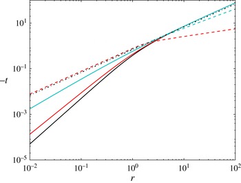
This then provides initial conditions for the numerical solution to (4.1) corresponding to outward-travelling waves for all ${\it\mu}\geqslant 0$ . We fix ${\it\gamma},{\it\mu}$ , choose $r=r_{0}\ll 1$ and calculate the initial condition $t(r_{0})$ from the above solutions. Figure 1 shows some trajectories for several ${\it\mu}$ . Except for ${\it\mu}=1$ , all trajectories show a change in gradient at around $r\simeq 10$ . When ${\it\mu}>1$ , solutions tend to the gas-dynamic asymptote when $r\rightarrow 0$ , and separate at larger radii. For ${\it\mu}<1$ , the converse is true. It is clear from the above that when $r\rightarrow 0$ , ${\it\mu}<1$ produces field-dominated solutions near the origin, while ${\it\mu}>1$ produces gas-dynamics-dominated solutions.

Figure 1.

Trajectories for the magnetosonic wave collapsing onto a power-law line current. Solid, bottom to top on the left: ${\it\mu}=0$ (black), ${\it\mu}=0.1$ (red), ${\it\mu}=0.5$ (cyan). Dashed, bottom to top on the right: ${\it\mu}=5$ (red), ${\it\mu}=1.5$ (cyan). Dash-dotted: ${\it\mu}=1$ .

4.1.2 Asymptotic solution, $r\rightarrow \infty$

Figure 1 suggests power-law behaviour for $r\rightarrow \infty$ . Again we construct a power-law ansatz for $t(r)$ , $r\rightarrow \infty$

(4.7) $$\begin{eqnarray}\displaystyle (-t)=A_{\infty }r^{{\it\nu}_{\infty }},\quad {\it\nu}_{\infty }>0,~A_{\infty }>0,~r\gg 1. & & \displaystyle\end{eqnarray}$$

Here when ${\it\mu}{\it\nu}_{\infty }-1>0$ , the $r$ or field term is dominant at infinity. Matching terms and enforcing assumptions then shows that this requires ${\it\mu}>1$ . Conversely, when ${\it\mu}{\it\nu}_{\infty }-1<0$ , the ${\it\gamma}$ term is dominant when $r\rightarrow \infty$ , which requires ${\it\mu}<1$ . A short calculation then gives that

(4.8a,b ) $$\begin{eqnarray}\displaystyle \left.A_{\infty }\right|_{{\it\mu}>1}=\left.A_{0}\right|_{{\it\mu}<1},\quad \left.A_{\infty }\right|_{{\it\mu}<1}=\left.A_{0}\right|_{{\it\mu}>1}, & & \displaystyle\end{eqnarray}$$

and

(4.9a,b ) $$\begin{eqnarray}\displaystyle \left.{\it\nu}_{\infty }\right|_{{\it\mu}>1}=\left.{\it\nu}_{0}\right|_{{\it\mu}<1},\quad \left.{\it\nu}_{\infty }\right|_{{\it\mu}<1}=\left.{\it\nu}_{0}\right|_{{\it\mu}>1}. & & \displaystyle\end{eqnarray}$$

From the above, for the converging magnetosonic wave we can draw the following conclusions:

1. (1) When $0\leqslant {\it\mu}<1$ , a wave is always gas-dynamics dominated far from the axis of convergence but becomes field dominated as it converges to the axis.

2. (2) When ${\it\mu}>1$ , a wave is always field dominated far from the axis but changes to become gas-dynamics dominated near the origin.

3. (3) For a given solution (meaning ${\it\gamma},{\it\mu}$ fixed), cross-over between the types of behaviour occurs in a range of $r$ where neither ${\it\gamma}$ nor $(-t)^{2{\it\mu}}/r^{2}$ is dominant in (4.1).

4. (4) For ${\it\mu}=1$ , a single, linear balanced, solution exists where there is no change-over region.

In the sequel we will consider finite-strength, fast-shock solutions which will be characterized according to their behaviour close to the origin. It will be seen that the type distinction between ${\it\mu}<1$ and ${\it\mu}>1$ seen for magnetosonic waves will be modified for converging fast magnetosonic shocks. In particular, the single magnetosonic balanced case ${\it\mu}=1$ , which separates magnetosonic-wave evolution will expand into a transition or cross-over zone in which solution properties depend on ${\it\mu}$ . As ${\it\mu}$ is increased from ${\it\mu}=0$ we will identify five regions of distinct behaviour. Within each region, solution properties will be seen to depend mainly on ${\it\mu}$ and the Whitham (Reference Whitham2011) parameter

(4.10) $$\begin{eqnarray}\displaystyle n({\it\gamma})=1+\frac{2}{{\it\gamma}}+\sqrt{\frac{2{\it\gamma}}{{\it\gamma}-1}}, & & \displaystyle\end{eqnarray}$$

as well as parametrically on ${\it\gamma}$ . While several properties of the shock collapse can be calculated explicitly, our present focus will be on $M(r)$ and the behaviour of the pressure $p(r)$ , $r\rightarrow 0$ .

4.2 Small $M-1$ approximation

4.2.1 Asymptotic solution, $r\rightarrow 0$ : Regions I and II

Pullin et al. (Reference Pullin, Mostert, Wheatley and Samtaney2014) showed that, for ${\it\mu}=0$ , the converging shock always weakens to $M=1$ with $p\rightarrow 1$ when $r\rightarrow 0$ . Coupled with our observation in § 4.1 that ${\it\mu}{\it\nu}_{0}<1$ shows field-dominated behaviour for the magnetosonic wave solution, we examine the behaviour of the GSD ODE pair (3.15) and (3.17) for ${\it\mu}{\it\nu}_{0}<1$ under the assumption of small Mach number. We thus introduce $m=M-1$ , with $m\ll 1$ , and use the secondary assumption that ${\it\epsilon}\rightarrow 0$ owing to field domination when $r\rightarrow 0$ .

For $m\ll 1$ , a series expansion of (3.5) and (3.7) for density and pressure around $m=0,{\it\epsilon}=0$ gives

(4.11) $$\begin{eqnarray}\displaystyle & \displaystyle {\it\rho}=1+\frac{4m}{3}+O(m^{2}); & \displaystyle\end{eqnarray}$$

(4.12) $$\begin{eqnarray}\displaystyle & \displaystyle p=1+\frac{4{\it\gamma}m}{3}+\frac{2{\it\gamma}(8{\it\gamma}-7)m^{2}}{27}+\frac{16{\it\gamma}({\it\gamma}-1)}{27}\frac{m^{3}}{{\it\epsilon}}+O\left(\frac{m^{4}}{{\it\epsilon}}\right), & \displaystyle\end{eqnarray}$$

where (4.12) has been expanded to third order to expose the $m^{3}/{\it\epsilon}$ term. This term may be finite or singular depending on the behaviour of $m(r),{\it\epsilon}(r)$ as $r\rightarrow 0$ , which is not known in advance. Hence, for MHD, small $m$ is not always associated with a weak shock in the sense of a small pressure jump: a small $m$ , strong-shock solution is admissible. In this approximation, the magnetosonic speed is thus defined as

(4.13) $$\begin{eqnarray}\displaystyle (c_{0})|_{{\it\mu}{\it\nu}_{0}<1,r\rightarrow 0,(-t)\rightarrow 0}\simeq \frac{(-t)^{{\it\mu}}}{r}, & & \displaystyle\end{eqnarray}$$

and so (3.15) can be written as

(4.14) $$\begin{eqnarray}\displaystyle \left(\frac{\text{d}t}{\text{d}r}\right)_{shock}\simeq -r(-t)^{-{\it\mu}}+O(mr(-t)^{-{\it\mu}}), & & \displaystyle\end{eqnarray}$$

which we may integrate to obtain $t(r)$ ,

(4.15) $$\begin{eqnarray}\displaystyle (-t)\simeq \left(\frac{{\it\mu}+1}{2}\right)^{1/({\it\mu}+1)}r^{2/({\it\mu}+1)}+\cdots \,,\quad r\rightarrow 0. & & \displaystyle\end{eqnarray}$$

This echoes the magnetosonic wave result (4.5) and again remains self-consistent for ${\it\mu}<1$ .

Substituting (4.15) and assuming a strong field with $m\ll 1$ , equation (3.17) may be expanded in a series and written to leading order as

(4.16) $$\begin{eqnarray}\displaystyle r\frac{\text{d}m}{\text{d}r}\simeq m\left(\frac{4-7{\it\mu}}{4({\it\mu}+1)}\right), & & \displaystyle\end{eqnarray}$$

which leads to

(4.17) $$\begin{eqnarray}\displaystyle m\simeq B_{2}r^{(4-7{\it\mu})/(4({\it\mu}+1))}. & & \displaystyle\end{eqnarray}$$

The exponent on $r$ in (4.17) remains positive only for ${\it\mu}<4/7$ , so that the asymptotic solution as a whole remains self-consistent only for $0<{\it\mu}<4/7$ .

A consequence of this behaviour of $m(r)$ may be exposed by examination of the $m^{3}/{\it\epsilon}$ term in (4.12). We note that ${\it\epsilon}$ may be written, using (4.13),

(4.18) $$\begin{eqnarray}\displaystyle {\it\epsilon}=\frac{a_{0}^{2}}{c_{0}^{2}}\simeq \frac{{\it\gamma}r^{2}}{(-t)^{2{\it\mu}}}\sim r^{2(1-{\it\mu})/(1+{\it\mu})}. & & \displaystyle\end{eqnarray}$$

Using this and (4.17) reveals that $m^{3}/{\it\epsilon}$ remains non-singular (but dominant in $p(r)-1$ ) for $0<{\it\mu}<4/13$ , which is denoted Region I, but becomes singular (and remains dominant in $p(r)$ ) for $4/13<{\it\mu}<4/7$ , denoted Region II. Using (4.17), equation (4.12) to leading order is

(4.19) $$\begin{eqnarray}\displaystyle & \displaystyle p(r)-1\sim r^{(4-13{\it\mu})/(4({\it\mu}+1))},\quad 0<{\it\mu}<4/13,(\text{Region I}), & \displaystyle\end{eqnarray}$$

(4.20) $$\begin{eqnarray}\displaystyle & \displaystyle p(r)\sim r^{(4-13{\it\mu})/(4({\it\mu}+1))},\quad 4/13<{\it\mu}<4/7,(\text{Region II}), & \displaystyle\end{eqnarray}$$

and $m$ given by (4.17) is non-singular in both regions. Physically, this result implies that as $r\rightarrow 0$ , the pressure behind the shock is non-singular in Region I but singular in Region II.

4.3 Large $M$ approximation

The previous analysis (§ 4.2) provided descriptions for field-dominated solutions close to the origin, and for both field- and gas-dynamics-dominated solutions far from the origin; however, there are possible solutions close to the origin with large Mach numbers which thus do not fall under that analysis. We now consider the strong shock approximation to the primary ODE (3.17). For $M\gg 1$ , the density and pressure jump conditions can be approximated to leading order as

(4.21) $$\begin{eqnarray}\displaystyle & \displaystyle {\it\rho}=\frac{{\it\gamma}+1}{{\it\gamma}-1}+O\left(\frac{1}{M^{2}}\right), & \displaystyle\end{eqnarray}$$

(4.22) $$\begin{eqnarray}\displaystyle & \displaystyle p=\frac{M^{2}}{{\it\epsilon}}\left(\frac{2{\it\gamma}}{{\it\gamma}+1}+O\left(\frac{1}{M^{2}}\right)\right)+O\left(\frac{1}{M^{2}}\right), & \displaystyle\end{eqnarray}$$

and the remaining jump conditions follow as usual. The ODE for the shock Mach number is now much simplified, but still very cumbersome.

4.3.1 Gas-dynamic strong shock: Region V

We consider first the gas-dynamics-dominated assumption, ${\it\mu}{\it\nu}_{0}>1$ , which simplifies the ODE further; other considerations ${\it\mu}{\it\nu}_{0}=1$ , ${\it\mu}{\it\nu}_{0}<1$ are discussed subsequently. The ansatz for shock trajectory close to the origin may be restated from (4.3), dropping subscripts,

(4.23) $$\begin{eqnarray}\displaystyle (-t)=Ar^{{\it\nu}},\quad r\ll 1. & & \displaystyle\end{eqnarray}$$

For ${\it\mu}{\it\nu}_{0}>1$ , and close to the origin, the magnetosonic speed becomes $c_{0}({\it\gamma})=\sqrt{{\it\gamma}}$ . Using (4.23) the shock-trajectory ODE (3.15), with (4.23), yields

(4.24) $$\begin{eqnarray}\displaystyle M=B_{3}r^{1-{\it\nu}},\quad B_{3}=\frac{1}{A{\it\nu}\sqrt{{\it\gamma}}}. & & \displaystyle\end{eqnarray}$$

Further, since $M\geqslant 1,r\rightarrow 0$ , this requires ${\it\nu}\geqslant 1$ for consistency; that is, $M$ converges to either a large constant or is singular as $r\rightarrow 0$ . The ODE (3.17) then reduces to

(4.25) $$\begin{eqnarray}\displaystyle r\frac{\text{d}M}{\text{d}r}=-{\displaystyle \frac{1}{n({\it\gamma})}}M+{\it\mu}\frac{(-t)^{-1+2{\it\mu}}}{r}K_{2}({\it\gamma}), & & \displaystyle\end{eqnarray}$$

where the second term on the right-hand side may be rewritten as $\propto \!r^{2{\it\mu}{\it\nu}-{\it\nu}-1}$ , since according to (4.23),

(4.26) $$\begin{eqnarray}\displaystyle \frac{(-t)^{-1+2{\it\mu}}}{r}=A^{2{\it\mu}-1}r^{2{\it\mu}{\it\nu}-{\it\nu}-1}. & & \displaystyle\end{eqnarray}$$

Now it can be seen that the first term on the right hand side of (4.25) dominates: both terms may be written as functions of $r$ (since $M\propto r^{1-{\it\nu}}$ ), but the term with the smallest (most negative) exponent dominates, and the second term may not dominate or balance with the first since $2{\it\mu}{\it\nu}-{\it\nu}-1<1-{\it\nu}$ requires ${\it\mu}{\it\nu}<1$ , which is inconsistent with the initial gas-dynamics-dominated assumption. (The second term is however singular close to the origin for ${\it\mu}<1$ without violation of ${\it\mu}{\it\nu}>1$ .) On neglecting the second term on the right-hand side of (4.25), this equation can be integrated to give, to leading order,

(4.27) $$\begin{eqnarray}\displaystyle M=B_{3}r^{-1/n({\it\gamma})}, & & \displaystyle\end{eqnarray}$$

where $n({\it\gamma})$ is given by (4.10), which matches Whitham’s result for the cylindrical, gas-dynamic strong shock limit. With $n(5/3)=4.43607$ , this gives an exponent $-0.225425$ . Comparing (4.27) with (4.24) then gives ${\it\nu}_{g}\equiv 1+1/n$ and ${\it\nu}_{g}(5/3)=1.225425$ . Our gas-dynamics-dominant assumption ${\it\mu}{\it\nu}>1$ then places a lower limit ${\it\mu}>n/(1+n)$ , which, for ${\it\gamma}=5/3$ gives ${\it\mu}>0.8160$ . This differs from the magnetosonic wave, where gas-dynamics dominated behaviour occurs only for ${\it\mu}>1$ ; the difference is due to the presence of $M$ in (3.15), and its absence in (4.4).

4.3.2 Field-dominated strong shock: Region IV

The field-dominated ( ${\it\mu}{\it\nu}<1$ ) strong-shock problem proceeds similarly. The magnetosonic speed is given by (4.13), so that using (4.23) and (3.15) as previously we obtain

(4.28) $$\begin{eqnarray}\displaystyle M=\frac{r^{2}}{{\it\nu}(-t)^{{\it\mu}+1}}=B_{4}r^{2-{\it\mu}{\it\nu}-{\it\nu}},\quad B_{4}={\displaystyle \frac{1}{(A^{{\it\mu}+1}{\it\nu})}}, & & \displaystyle\end{eqnarray}$$

where for consistency we require $2-{\it\mu}{\it\nu}-{\it\nu}<0$ to allow for growth of $M$ as $r\rightarrow 0$ . Expanding the right-hand side of (3.17) and retaining leading-order terms gives, for the field-dominated case

(4.29) $$\begin{eqnarray}\displaystyle r\frac{\text{d}M}{\text{d}r}=\left(1-{\displaystyle \frac{1}{n({\it\gamma})}}\right)M-\frac{{\it\mu}r^{2}}{(-t)^{{\it\mu}+1}}. & & \displaystyle\end{eqnarray}$$

Using (4.28), equation (4.29) becomes

(4.30) $$\begin{eqnarray}\displaystyle r\frac{\text{d}M}{\text{d}r}=M\left(1-{\displaystyle \frac{1}{n}}-{\it\mu}{\it\nu}\right), & & \displaystyle\end{eqnarray}$$

with solution

(4.31) $$\begin{eqnarray}\displaystyle M=B_{4}r^{1-(1/n)-{\it\mu}{\it\nu}}. & & \displaystyle\end{eqnarray}$$

Matching exponents between (4.28) and (4.31) provides ${\it\nu}=1+1/n({\it\gamma})$ and so

(4.32) $$\begin{eqnarray}\displaystyle M=B_{4}r^{1-(1/n)-{\it\mu}\left(1+1/n\right)}. & & \displaystyle\end{eqnarray}$$

The condition for field-dominated behaviour ${\it\mu}{\it\nu}={\it\mu}{\it\nu}_{g}<1$ sets ${\it\mu}<1/{\it\nu}$ , and the condition for singular $M$ as $r\rightarrow 0$ sets ${\it\mu}>2/{\it\nu}-1=(1-1/n)/(1+1/n)\simeq 0.632$ for ${\it\gamma}=5/3$ . Therefore, singular solutions exist for $M(r)$ as $r\rightarrow 0$ for the field-dominated case for $(n-1)/(n+1)<{\it\mu}<n/(n+1)$ with a Mach number exponent that depends on ${\it\mu}$ . This is defined as Region IV. When ${\it\mu}=n/(n+1)$ the exponent in (4.32) equals $-1/n({\it\gamma})$ which matches that in Region V. In Region IV, ${\it\epsilon}\sim r^{2(1-{\it\mu})/({\it\mu}+1)}$ , and so

(4.33) $$\begin{eqnarray}\displaystyle p(r)\sim r^{2({\it\mu}n(1-{\it\mu})-({\it\mu}+1)^{2})/(n({\it\mu}+1))} & & \displaystyle\end{eqnarray}$$

which is always singular.

4.3.3 Balanced strong shock: Region IVb

In the balanced strong-shock problem, thermodynamic and magnetic contributions to $c_{0}$ remain in balance as the shock collapse to the origin ( ${\it\mu}{\it\nu}=1$ ). Then, by (4.3),

(4.34) $$\begin{eqnarray}\displaystyle c_{0}=\sqrt{{\it\gamma}+A^{2{\it\mu}}}, & & \displaystyle\end{eqnarray}$$

and the rest of the analysis proceeds similarly to the gas-dynamics-dominated case. Ultimately we obtain

(4.35) $$\begin{eqnarray}\displaystyle M=B_{5}r^{1-{\it\nu}},\quad B_{5}={\displaystyle \frac{{\it\mu}}{(A\sqrt{{\it\gamma}+A^{2{\it\mu}}})}}. & & \displaystyle\end{eqnarray}$$

For ${\it\gamma}=5/3$ , ${\it\nu}={\it\nu}_{g}=1+1/n$ and ${\it\mu}=n/(n+1)$ by the balanced assumption.

The strong shock regions can then be denoted as follows:

(4.36) $$\begin{eqnarray}\displaystyle & \displaystyle M(r)\propto r^{1-(1/n)-{\it\mu}\left(1+1/n\right)},\quad \frac{n-1}{n+1}<{\it\mu}<\frac{n}{n+1},(\text{Region IV}); & \displaystyle\end{eqnarray}$$

(4.37) $$\begin{eqnarray}\displaystyle & \displaystyle M(r)\propto r^{-1/n},\quad {\it\mu}=\frac{n}{n+1},(\text{Region IVb}); & \displaystyle\end{eqnarray}$$

(4.38) $$\begin{eqnarray}\displaystyle & \displaystyle M(r)\propto r^{-1/n},\quad {\it\mu}>\frac{n}{n+1},(\text{Region V}); & \displaystyle\end{eqnarray}$$

and the pressure behind the shock is singular and proportional to $M^{2}/{\it\epsilon}$ by (4.22). For Regions IVb and V, however, since ${\it\epsilon}$ does not approach zero where $r\rightarrow 0$ , then $p\sim M^{2}\sim r^{-2/n}$ .

4.4 Convergent Mach number analysis: Region III

For ${\it\gamma}$ less than the physically unrealistic value ${\it\gamma}=2.4299$ (which satisfies $(n({\it\gamma})-1)(n({\it\gamma})+1)=4/7$ ), the lower bound on ${\it\mu}$ for the field-dominated, strong shock solution does not extend to the upper bound on ${\it\mu}$ of Region II. There is thus a gap in the range $4/7<{\it\mu}<(n-1)/(n+1)$ where neither the weak-shock nor the strong-shock analysis may be appropriate. This range is denoted Region III and is now addressed.

We hypothesize that here $M(r)\rightarrow M_{1}>1$ as $r\rightarrow 0$ . To test this we first assume field-dominated behaviour: ${\it\mu}{\it\nu}_{0}<1$ . This is done since Regions I, II and IV all self-consistently follow field-dominated assumptions. Equation (4.13) then supplies $c_{0}$ , as usual for this assumption. Second, we assume the Mach number variation in Region III

(4.39) $$\begin{eqnarray}\displaystyle M(r)=M_{1}+Dr^{{\it\delta}}+\text{HOT},\quad r\rightarrow 0, & & \displaystyle\end{eqnarray}$$

where $M_{1}=M_{1}({\it\mu})\geqslant 1$ and ${\it\delta}={\it\delta}({\it\mu})>0$ are to be determined, and $D$ is a constant which depends on initial conditions. This is consistent with our analysis of Regions I and II where $M_{1}=1$ and ${\it\delta}({\it\mu})=(4-7{\it\mu})/(4({\it\mu}+1))$ . Equation (4.39) may then be substituted into (3.15), which is integrated to obtain

(4.40) $$\begin{eqnarray}\displaystyle \frac{(-t)^{{\it\mu}+1}}{{\it\mu}+1}=\frac{r^{2}\text{}_{2}F_{1}\left(1,{\displaystyle \frac{2}{{\it\delta}}};1+{\displaystyle \frac{2}{{\it\delta}}};-{\displaystyle \frac{Dr^{{\it\delta}}}{M_{1}}}\right)}{2M_{1}}, & & \displaystyle\end{eqnarray}$$

where $_{2}F_{1}(a,b;c;z)$ is the hypergeometric function. A series expansion to two terms gives

(4.41) $$\begin{eqnarray}\displaystyle (-t)\simeq \left(\frac{{\it\mu}+1}{2M_{1}}-\frac{({\it\mu}+1)Dr^{{\it\delta}}}{(2+{\it\delta})M_{1}^{2}}\right)^{1/({\it\mu}+1)}r^{2/({\it\mu}+1)}, & & \displaystyle\end{eqnarray}$$

which may also be written in terms of $M(r)$ and $r$ , using (4.39),

(4.42) $$\begin{eqnarray}\displaystyle (-t)\simeq \left(\frac{{\it\mu}+1}{2M_{1}}-\frac{({\it\mu}+1)(M-M_{1})}{(2+{\it\delta})M_{1}^{2}}\right)^{1/({\it\mu}+1)}r^{2/({\it\mu}+1)}. & & \displaystyle\end{eqnarray}$$

Equation (4.42) can then be substituted into the GSD ODE (3.17) to remove the dependency on $t$ . Premultiplying by $r$ then gives

(4.43) $$\begin{eqnarray}\displaystyle r\frac{\text{d}M}{\text{d}r}=\mathscr{F}(r,M,M_{1},{\it\delta},{\it\mu},{\it\gamma}), & & \displaystyle\end{eqnarray}$$

where $\mathscr{F}$ is a known but very complicated function of its arguments.

Consistency with (4.39) requires that the right-hand side of (4.43) is zero when $r\rightarrow 0$ . Noting also that in this limit, when $M\rightarrow M_{1}$ , the dependence on ${\it\delta}$ vanishes then gives

(4.44) $$\begin{eqnarray}\displaystyle \lim _{r\rightarrow 0}\left.\mathscr{F}(r,M,M_{1},{\it\delta},{\it\mu},{\it\gamma})\right|_{M=M_{1}}\equiv \mathscr{G}(M_{1},{\it\mu},{\it\gamma})=0, & & \displaystyle\end{eqnarray}$$

where $\mathscr{G}$ is a known function. Equation (4.44) can be solved for $M_{1}$ for a particular ${\it\mu}$ (setting ${\it\gamma}=5/3$ ) using a root-finding method. Applying now the left-hand side of (4.43) to (4.39), and taking the partial derivative with respect to $M$ , setting $M=M_{1}$ and then taking the limit $r\rightarrow 0$ gives

(4.45) $$\begin{eqnarray}\displaystyle \left.\lim _{r\rightarrow 0}\frac{\partial \mathscr{F}(r,M,M_{1},{\it\delta},{\it\mu},{\it\gamma})}{\partial M}\right|_{M=M_{1}}=\mathscr{P}(M_{1},{\it\delta},{\it\mu},{\it\gamma})={\it\delta}, & & \displaystyle\end{eqnarray}$$

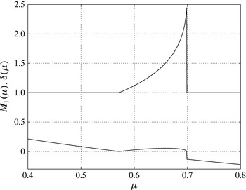
where $\mathscr{P}$ is a known function of its arguments. The equation $\mathscr{P}(M_{1},{\it\delta},{\it\mu},{\it\gamma})-{\it\delta}=0$ can be solved numerically for ${\it\delta}$ given $M_{1}({\it\mu})$ found from (4.44). The variation of ${\it\delta}({\it\mu})$ is shown by the lower curve in figure 2; in Regions I and II, ${\it\delta}({\it\mu})$ here agrees with the exponent in (4.17) from the weak shock approximation, but is valued negative real for $(n-1)/(n+1)<{\it\mu}<1$ .

This method remains self-consistent up to a ${\it\mu}_{III}={\it\mu}_{III}({\it\gamma})$ , with ${\it\mu}_{III}(5/3)=0.699$ . There is then an overlap between Regions III and IV in the range $(n-1)/(n+1)<{\it\mu}<{\it\mu}_{III}$ . In this overlap region, numerical solutions to the full GSD ODEs (to be described) indicate that the solution approaches an asymptote that is either Region-III-like or Region-IV-like, depending on ${\it\mu}$ and the initial conditions, and that there is a cross-over Mach number $M_{c}=M_{c}({\it\mu})$ at $r_{0}=1$ which separates these solutions. This means that for $M_{0}<M_{c}({\it\mu})$ , we expect $M(r)$ to asymptote to a constant value when $r\rightarrow 0$ (Region-III like), while for $M_{0}>M_{c}({\it\mu})$ , we expect $M(r)$ to approach the asymptote (4.32) (Region-IV like). Also it is clear that when ${\it\mu}\rightarrow (n-1)/(n+1)$ from above, then $M_{c}({\it\mu})\rightarrow \infty$ while when ${\it\mu}\rightarrow {\it\mu}_{III}$ from below, then $M_{c}({\it\mu})\rightarrow 1$ . As an example, at ${\it\mu}=0.65$ , $M_{c}\simeq 2.5$ at $r_{0}=1$ . The overlap region covers a small range of ${\it\mu}$ and cannot be fully analysed by asymptotic analysis. It is not considered further.

Figure 2.

Variation of $M_{1}({\it\mu})$ (upper) and ${\it\delta}({\it\mu})$ (lower), from (4.39), for $0.4<{\it\mu}<0.8$ . The function is valued greater than unity for $4/7<{\it\mu}<0.699$ .

Table 1.

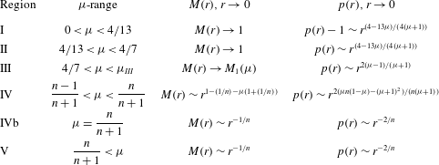
Summary of asymptotic behaviour of Mach number $M(r)$ and pressure $p(r),r\rightarrow 0$ obtained from GSD. Regions I–IVb are considered as field-dominated shock convergence. Note that there exists overlap between Regions III and IV over the range $(n-1)/(n+1)<{\it\mu}<{\it\mu}_{III}$ . For ${\it\gamma}=5/3$ , this is $0.632<{\it\mu}<0.699$ . The dependence of ${\it\mu}_{III}({\it\gamma})$ has not been determined. For Regions I–III, $t(r)\sim r^{({\it\mu}+1)/2}$ ; for Regions IV–V, $t(r)\sim r^{{\it\nu}_{g}}$ , ${\it\nu}_{g}=1+1/n({\it\gamma})$ where $n({\it\gamma})$ is given by (4.10).

4.4.2 Asymptotic solutions, $r\rightarrow \infty$

We complete this section by considering the behaviour of solutions to the GSD ODE when $r\rightarrow \infty$ . This can be done using a small-Mach-number approximation as in § 4.2. As was observed in § 4.1.2, when $r\rightarrow \infty$ , the behaviour of the magnetosonic wave is opposite to its behaviour close to the origin; that is, for ${\it\mu}<1$ , the magnetosonic wave is field-dominated near $r=0$ but gas-dynamics dominated as $r\rightarrow \infty$ , and vice versa for ${\it\mu}>1$ . Here we investigate the behaviour of a finite-strength shock far from the origin. We again use the $m\ll 1$ of the shock-jump conditions. The field-dominated case corresponds to ${\it\mu}{\it\nu}_{\infty }<1$ . Noting that ${\it\nu}_{\infty ,{\it\mu}>1}={\it\nu}_{0,{\it\mu}<1}$ from § 4.1, the analysis proceeds as in § 4.4.2: by assuming $m\ll 1$ , we reproduce (4.15)–(4.17), this time under the conditions $r\gg 1$ , ${\it\mu}>1$ .

For $r\rightarrow \infty$ , for a strong field and weak shock, we find that, similarly to the magnetosonic wave case, with ${\it\mu}>1$ , (4.15) holds. Following a similar approach to the $r\rightarrow 0$ asymptotic solution above, we may also reproduce (4.17). The exponent on $r$ in (4.17) is negative for all ${\it\mu}>1$ , so that $m\rightarrow 0$ as $r\rightarrow \infty$ as given by this equation with ${\it\mu}>1$ .

For the weak-field or gas-dynamic-dominated case, with $r\rightarrow \infty$ , $c_{0}\simeq r/\sqrt{{\it\gamma}}$ . Here we substitute (4.11) into the exact pressure equation (3.7) and perform a series expansion around $m=0$ on the result. To leading order, this gives

(4.46) $$\begin{eqnarray}\displaystyle m\simeq B_{2}r^{-1/2}, & & \displaystyle\end{eqnarray}$$

where $B_{2}$ is a constant of integration depending on initial conditions. By comparison with the magnetosonic wave case far from the origin, this analysis remains consistent for ${\it\mu}<1$ (since ${\it\nu}_{\infty }=1$ ).

5.1 Geometrical shock dynamics

We now turn to finding solutions numerically to the system of ODEs (3.17) and (3.15) over a finite range of $r$ . From the asymptotic analysis we expect that, for fixed ${\it\gamma}$ , there will exist a two-parameter family of solutions characterized by ${\it\mu}\geqslant 0$ and an initial Mach number $M_{0}>1$ at some fixed radius $r_{0}$ . We also require an initial condition $t_{0}$ which must satisfy (3.21). If $t_{0}$ is the collapse time for given $(r_{0},M_{0})$ , then we expect $t_{0}=t_{0}(M_{0},r_{0};{\it\mu},{\it\gamma})$ . The parameter $0<r_{0}<\infty$ is arbitrary and, for the purposes of numerical solutions, we presently choose $r_{0}=100$ . Once $t_{0}$ is known for given $M_{0},r_{0};{\it\mu},{\it\gamma}$ , its value for any $r$ can be obtained by integrating the GSD ODE pair in $r$ from these initial conditions. We remark that the ODE pair can in fact be successfully integrated reversibly in any finite range of $r$ even though solutions have physical meaning as a shock-wave evolution for decreasing $r$ . Presently we use a root-finding method for solving the shooting problem (3.17) and (3.15) subject to (3.21). An alternative is to use the asymptotic solutions described previously to manufacture initial conditions close to $r=0$ and then solve the ODE pair outwards. This method will be described later for the verification of asymptotic solutions within each region. For more general cases, a robust methodology for finding $t_{0}$ is preferred. The method used presently was implemented using the ODE-solving capability provided in MATHEMATICA. The numerical details are outlined in appendix B.

5.2 Finite volume method for full MHD PDE system

Here we verify our GSD formulation by comparing GSD numerical solutions with solutions of the full one-dimensional unsteady PDE system describing the shock collapse. The latter do not rely on the GSD assumptions, but, owing to the singular behaviour of both the magnetic field ahead of the shock and also of the collapse evolution of some solutions, are not well suited to characterizing the final stages of shock collapse. Further, it is difficult to implement the shock collapse condition (3.21) into PDE simulations. Nonetheless solutions of the MHD PDE system are required to presently verify our time-domain GSD approach.

The solution method is described in detail in Samtaney et al. (Reference Samtaney, Colella, Ligocki, Martin and Jardin2005). The one-dimensional equations in conservation form are

(5.1) $$\begin{eqnarray}\displaystyle \frac{\partial U}{\partial t}+\frac{1}{r}\frac{\partial (rF)}{\partial r}=S, & & \displaystyle\end{eqnarray}$$

where $U=\{{\it\rho},{\it\rho}u,B_{{\it\theta}},e\}^{\text{T}}$ , where $e$ is the total energy per unit volume. Note that here we are using the energy equation in place of the entropy equation used in (2.4), which are equivalent for inviscid, non-dissipative MHD. The flux $F(U)$ and source $S(U)$ are given by

(5.2) $$\begin{eqnarray}\displaystyle F(U) & = & \displaystyle \left\{{\it\rho}u,{\it\rho}u^{2}+p^{\ast },B_{{\it\theta}}u,(e+p_{t})u\right\}^{\text{T}},\end{eqnarray}$$

(5.3) $$\begin{eqnarray}\displaystyle S(U) & = & \displaystyle \frac{1}{r}\left\{0,p^{\ast }-B_{{\it\theta}}^{2},r\,\text{d}B_{{\it\theta},0}/\text{d}t+B_{{\it\theta}}u,0\right\}^{\text{T}},\end{eqnarray}$$

where the magnetic pressure $p^{\ast }$ is given by (2.9). The total energy $e$ is related to the pressure as follows:

(5.4) $$\begin{eqnarray}\displaystyle e=\frac{p}{{\it\gamma}-1}+\frac{1}{2}{\it\rho}u^{2}+\frac{1}{2}(B_{{\it\theta}}^{2}+B_{z}^{2}). & & \displaystyle\end{eqnarray}$$

The present version of the numerical method is summarized in Pullin et al. (Reference Pullin, Mostert, Wheatley and Samtaney2014). Briefly, the above equations are modified by subtracting out the singular magnetic field, writing the azimuthal component as $B_{{\it\theta}}=B_{{\it\theta},0}+B_{{\it\theta},1}$ , with $B_{{\it\theta},0}=(-t)^{{\it\mu}}/r$ . This enables cancellation of terms that vary as $r^{-3}$ in the radial momentum equation, thus alleviating large numerical errors that would otherwise arise near $r=0$ . The modified equations are solved by a finite volume upwind method (Samtaney et al. Reference Samtaney, Colella, Ligocki, Martin and Jardin2005). Here the radial domain is discretized into finite volumes and an exponentially stretched mesh is used in the radial direction which concentrates volume elements near the origin. A predictor–corrector method is utilized wherein we first predict the solution at time $n+(1/2)$ at finite volume faces using a combination of Taylor series expansion of fluxes together with linear profiles in each computational cell that are limited in the space of characteristic variables using Van Leer slope limiting. This gives left and right predicted states at volume interfaces and the local solution is then obtained using a standard multi-wave, linearized solver for the Riemann problem. This allows direct computation of the numerical fluxes at volume interfaces and the solution is then updated in each finite volume. The computer code includes an optional, explicit second-derivative artificial viscosity term used to filter grid-level oscillations if present. Prior verification testing has been performed on linear wave propagation, magnetic reconnection (Samtaney et al. Reference Samtaney, Colella, Ligocki, Martin and Jardin2005) and regular shock refraction at a density interface in MHD (Wheatley, Pullin & Samtaney Reference Wheatley, Pullin and Samtaney2005) while convergence testing is described by Wheatley et al. (Reference Wheatley, Samtaney and Pullin2009, Reference Wheatley, Samtaney, Pullin and Gehre2014). We will subsequently describe these solutions as computational MHD (CMHD) solutions, to be distinguished from numerical GSD solutions.

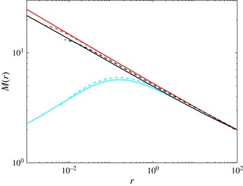
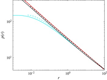
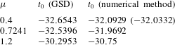
We compare GSD solutions with CMHD solutions for ${\it\mu}=0.4,0.7241$ and $1.2$ , which correspond to Regions II, IV and V respectively, with $r_{0}=100,~M_{0}=2$ . Figure 3 shows Mach number for each solution type, and figure 4 the pressure behind the shock. The CMHD and GSD solutions show general agreement in these variables. The ${\it\mu}=0.4$ case exhibits the greatest difference with the peak Mach number differing by $4.5\,\%$ (normalized by the numerical solution), and the maximum pressure difference, at $r=10^{-2}$ , by $14.5\,\%$ . These are of similar order to the discrepancies seen in table II of Pullin et al. (Reference Pullin, Mostert, Wheatley and Samtaney2014).

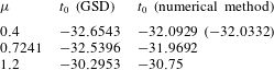
The initial condition $t_{0}$ is difficult to tune to the shock collapse time using the CMHD method. However, the difference between the CMHD estimate and the GSD estimate of $|t_{0}|$ is at most 1.9 %. Collapse times from both methods for the solutions shown in figures 3 and 4 are shown in table 2.

Figure 3.

Comparison of Mach number between numerical, geometrical shock dynamics (GSD) solutions and tuned computational MHD (CMHD) solutions to the full one-dimensional unsteady MHD PDEs. Solid: GSD solutions. Dashed: CMHD solutions. Bottom to top; ${\it\mu}=0.4$ (cyan), ${\it\mu}=0.7241$ (black), ${\it\mu}=1.2$ (red).

Figure 4.

Comparison of pressure behind the shock between numerical GSD and CMHD solutions. Key as in figure 3.

Table 2.

Collapse times from $r_{0}=100$ estimated by the numerical GSD solutions CMHD solutions. Parenthetical value for ${\it\mu}=0.4$ indicates an estimate using a doubled resolution mesh. Here $M_{0}=2,~r_{0}=100$ .

6.1 Mach number variation

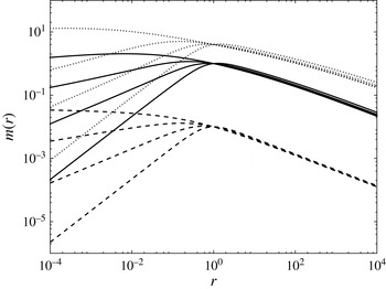
The variation of Mach number $M(r)$ over radius is shown in figures 5 and 6 for a variety ${\it\mu}$ in Regions I–III and IV–V, respectively, for initial conditions $r_{0}=1$ , $M_{0}=1.01$ , $M_{0}=2.0$ and $M_{0}=5.0$ . The ${\it\mu}$ are chosen to reflect each region of behaviour: ${\it\mu}=0,~0.2~\text{(I)},~0.4~\text{(II)},~0.6~\text{(III)},~0.7~\text{(IV)},~0.9~\text{(V)}$ . All solutions $M(r)$ in Regions I and II are clearly regular when $r\rightarrow 0$ . They appear to converge to unity Mach number, an observation which supports the reduced analyses performed in § 4.2. The Region III solutions also do not appear to be singular, particularly for $M_{0}=2.0,5.0$ . Figure 5 suggests that the solutions in Regions I and II (and the ${\it\mu}=0$ case) have reached their $r\rightarrow 0$ asymptotes. These asymptotics have different power-law variations, and follow the predicted ${\it\delta}({\it\mu})$ from the weak shock analysis in § 4.2. The Region III solution has not reached its $r\rightarrow 0$ asymptote by the lowest decades in $r$ on the figure.

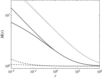
Figure 6 shows that Regions IV and V, however, both show singular Mach number growth as $r\rightarrow 0$ , as predicted by the strong-shock analyses in § 4.3. For the Region IV case, this is most clear for $M_{0}=2.0,5.0$ . Region V appears singular in all provided solutions.

Figure 5.

Mach number $m(r)=M(r)-1$ . Dashed: $M_{0}=1.01$ at $r_{0}=1$ . Solid: $M_{0}=2.0$ . Dotted: $M_{0}=5.0$ . In each set, ${\it\mu}=0,0.2,0.4,0.6$ from bottom to top.

Figure 6.

Mach number $M(r)$ for sets of initial conditions as in figure 5. In each set, ${\it\mu}=0.7$ on the lower curve and ${\it\mu}=0.9$ on the upper.

Figure 7.

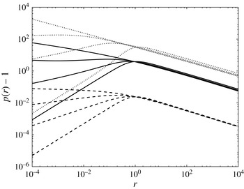
Pressure curves $p(r)-1$ for solutions in Regions I–III. In each set from bottom to top: ${\it\mu}=0.0,0.2,0.4,0.6$ . Line styles as in previous figures. The upper curve in each set (Region III) is singular.

Figure 8.

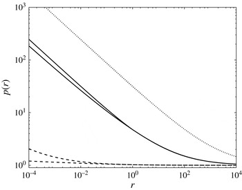
Singular pressure curves for solutions in Regions IV and V. Here ${\it\mu}=0.7$ on the lower curve of each set; ${\it\mu}=0.9$ on the upper. Line styles as in previous figures. For the $M_{0}=5.0$ case (dotted), the two pressure curves collapse across all plotted $r$ .

6.2 Pressure variation

In the context of cylindrical converging shock waves in fusion applications such as MagLIF (Sefkow et al. Reference Sefkow, Slutz, Koning, Marinak, Peterson, Sinars and Vesey2014), this property of gas-dynamic behaviour near the origin in the presence of a magnetic field could allow the simultaneous potentially beneficial effects of the seed magnetic field on hydrodynamic instabilities such as Richtmyer–Meshkov or Rayleigh–Taylor, while remaining strong, in the sense of both pressure and Mach number, as it approaches the origin. This potentially obviates the difficulty noted in Pullin et al. (Reference Pullin, Mostert, Wheatley and Samtaney2014), where (in what is the ${\it\mu}=0$ case here) the shock weakened to a magnetosonic wave as it approached the origin. Figures 7 and 8 show pressure profiles for the same solutions as in figures 5 and 6. In these cases, the pressure profiles for Regions I, IV and V follow qualitatively the behaviour of the corresponding $M(r)$ curves. In Region III the pressure variation is clearly singular in contrast to the Region III $M(r)$ solution, which is non-singular (see figure 5). The Region II pressure is also singular; this is particularly visible in the $M_{0}=2.0,5.0$ curves.

Region I is then essentially similar to Pullin et al.’s case. A singular (or at least strong) pressure may be achieved at the origin by ensuring a sufficiently rapid field decay for a tuned shock (in the sense that the field decreases to zero precisely as the shock converges on the origin), such that ${\it\mu}$ is in one of Regions II–V. In Regions IV–V, a singular Mach number may additionally be ensured.

Figure 9.

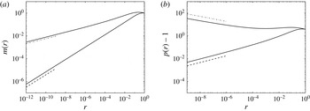
Geometrical shock dynamics numerical solutions in Regions I and II compared with $r\rightarrow 0$ asymptotics for Mach number $m(r)=M(r)-1$ and pressure $p(r)-1$ , using the outward solution technique: (a) $m(r)=M(r)-1$ ; (b) $p(r)-1$ . Solid lines: full solutions; from bottom to top, ${\it\mu}=0.2,0.4$ . Dashed: ${\it\mu}=0.2$ asymptote. Dash-dotted: ${\it\mu}=0.4$ asymptote.

6.3 Comparison of GSD numerical solutions with $r\rightarrow 0$ asymptotic results

For a given ${\it\mu}$ , as an alternative to the inward-integrated solution technique described in § 5.1, a GSD numerical solution can be generated by using an asymptotic $r\rightarrow 0$ result from § 4 to construct an initial condition extremely close to the origin. The GSD ODE pair can then be integrated outward in radius. To do this, we choose ${\it\mu}$ and a small initial radius such as $r_{0}=10^{-16}$ , and seek the associated time $t_{0}(r_{0},{\it\mu})$ and Mach number $M_{0}(r_{0},{\it\mu})$ . If we assume the initial conditions $r_{0},t_{0},M_{0}$ lie on an asymptotic $r\rightarrow 0$ solution in a given region, we may use one of (4.15), (4.41), (4.23) to define $t_{0}$ and one of (4.17), (4.39), (4.27), (4.32) to define $M_{0}$ , depending on the chosen ${\it\mu}$ and corresponding region. In setting these initial conditions, care should be taken that any additional assumptions taken in producing the asymptotic solution, for example small $m$ and strong field strength in Region I, are reasonably satisfied. Finally, in choosing the initial conditions, there is always a (single) free parameter which needs to be set; this is in principle arbitrary but should again be chosen to justify the asymptotic assumptions. We remark that with this method the collapse time is effectively set by the initial conditions but one cannot guarantee a priori a given $M_{0}$ at a given $r_{0}=1$ .

Once the initial conditions are defined, the GSD ODE may be solved outwards (that is, away from the origin) and compared with the corresponding asymptote. Figures 9 and 10 show comparisons for Mach number and pressure for each respective region. Good agreement is shown in all regions for Mach number, and especially in Regions I, II and V in pressure. In Regions III and IV, it is difficult even with the described outward-solution technique to produce initial conditions which lie on the respective asymptotic solution. This is because $c_{0}$ becomes very large, according to the field-dominated assumption, at such small $r$ so as to introduce numerical difficulties with integration of the GSD ODE.

Figure 10.

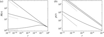
Geometrical shock dynamics solutions in Regions III–V compared with $r\rightarrow 0$ asymptotics, Mach number $M(r)$  (a) and pressure $p(r)$  (b). Solid lines: full solutions; from bottom to top, ${\it\mu}=0.6,0.7,0.9$ . Dashed: ${\it\mu}=0.6$ asymptote (set to constant value $M_{1}=1.1191$ ). Dash-dotted: ${\it\mu}=0.7$ asymptote, $p(r)$ . Dotted: ${\it\mu}=0.9$ asymptote. The Region III ( ${\it\mu}=0.6$ ) solution has not yet reached its asymptotic solution by the lowest decade for either variable.