



1. Introduction
Inspired by the multi-jet propulsion used by salps (Sutherland & Madin Reference Sutherland and Madin2010; Sutherland & Weihs Reference Sutherland and Weihs2017) and siphonophores (Costello et al. Reference Costello, Colin, Gemmell, Dabiri and Sutherland2015; Du Clos et al. Reference Du Clos, Gemmell, Colin, Costello, Dabiri and Sutherland2022), scalable marine robotic swarms that use multiple jets have been considered a promising direction for engineering development (Gemmell et al. Reference Gemmell, Dabiri, Colin, Costello, Townsend and Sutherland2021; Jiang et al. Reference Jiang, Costello and Colin2021; Wang et al. Reference Wang, Zhang, Zhang, Liu, Li, Chen, Deng and Liu2024). Compared with single-jet propulsion, this approach offers several advantages, including enhanced manoeuvrability and the ability to optimise propulsive performance across different tasks through different operational strategies (Du Clos et al. Reference Du Clos, Gemmell, Colin, Costello, Dabiri and Sutherland2022). However, the use of multiple jets inevitably introduces interactions between adjacent starting jets, which can significantly affect the overall propulsive characteristics. Additionally, the interactions between adjacent starting jets are also important in the design of synthetic jet actuators (Watson et al. Reference Watson, Jaworski and Wood2003; Liu et al. Reference Liu, Ji, Wang, Yu and Shan2024) and in medical applications such as edge-to-edge mitral valve repair (Alfieri et al. Reference Alfieri, Maisano, De Bonis, Stefano, Torracca, Oppizzi and La Canna2001; Sargordi et al. Reference Sargordi, Chtchetinina, Di Labbio, Ng and Kadem2020). To better understand these interactions, Athanassiadis & Hart (Reference Athanassiadis and Hart2016) first examined the influence of the interactions between two identical starting jets (referred to as twin-starting jets) on the thrust generation for a foundational insight. Subsequently, Zhu et al. (Reference Zhu, Zhang, Yu, Gao and Fan2026b ) conducted a more systematic investigation to reveal the underlying mechanisms of the twin-starting jet interactions.
In the investigations by Athanassiadis & Hart (Reference Athanassiadis and Hart2016) and Zhu et al. (Reference Zhu, Zhang, Yu, Gao and Fan2026b
), the analysis was simplified by considering two starting jets that initiate simultaneously from coplanar nozzle exits. In addition to the vortex-ring interactions suggested by Athanassiadis & Hart (Reference Athanassiadis and Hart2016), the mutually induced pressure (MIP) was identified as a dominant mechanism governing the interactions of twin-starting jets during the acceleration and deceleration stages. The vortex-ring interactions are mainly manifested in the interaction between the two leading vortex rings, which play a dominant role, as well as in their subsequent interaction with the stopping vortex rings. These interactions can be classified into two regimes based on the nozzle spacing
 $S/D$
, where
 $S$
is the distance between the axes of the two nozzles and
 $D$
is the nozzle diameter. In the first regime of
 $S/D \gt 1.5$
, the vortex rings remain intact and independent throughout the interaction process. The vortex-ring interactions in this regime are denoted as the coupling effects of vortex rings (CEVR). The theoretical models established for vortex rings (Athanassiadis Reference Athanassiadis2016; Athanassiadis & Hart Reference Athanassiadis and Hart2016) can be applied. In the second regime with smaller
 $S/D \lt 1.5$
, the reconnection occurs between the two leading vortex rings, resulting in complex three-dimensional vortical structures. The vortex-ring interactions in this regime are denoted as CEVR with reconnection. Notably, both regimes break the local axisymmetry about their respective jet axes, while the overall vortical wake of the twin-starting jets preserves global planar symmetry. Furthermore, the dominant mechanism of MIP remains consistent within the range of
 $1.1 \leqslant S/D \leqslant 4$
and can be described by the MIP model developed by Zhu et al. (Reference Zhu, Zhang, Yu, Gao and Fan2026b
). In terms of propulsive characteristics, twin-starting jet interactions not only reduce the average thrust, as suggested by Athanassiadis & Hart (Reference Athanassiadis and Hart2016), but also introduce additional fluctuations into the transient development of thrust. The interaction also disturbs the pressure field on the nozzle outer walls and generates lateral forces perpendicular to the jet direction. The forces on the two nozzle outer walls are equal in magnitude and opposite in direction, with a magnitude comparable to the axial thrust. However, reflecting on the biological inspiration for studying the interactions between twin-starting jets, i.e. the swimming of siphonophores (figure 1
a), it may be necessary to explore scenarios where the assumptions in Athanassiadis & Hart (Reference Athanassiadis and Hart2016) and Zhu et al. (Reference Zhu, Zhang, Yu, Gao and Fan2026b
), i.e. twin-starting jets initiated simultaneously with coplanar nozzle exits, are no longer valid.
Illustration of siphonophore morphology: (a) relevant features and (b) jetting and refilling states along with the positions of the velum and jet (reproduced from Du Clos et al. Reference Du Clos, Gemmell, Colin, Costello, Dabiri and Sutherland2022); and (c) distribution of nectophores in the propulsive component (reproduced from Costello et al. Reference Costello, Colin, Gemmell, Dabiri and Sutherland2015).

Figure 1. Long description
Panel A: A diagram of a siphonophore showing its relevant features. The siphonophore is divided into a nectosome and a siphosome. The nectosome contains nectophores labeled from 1L to 7R and a pneumatophore at the top. Panel B: A series of images showing the jetting and refilling states of a nectophore. The resting state, jetting state, and refill state are depicted, with the velum and jet positions indicated. Panel C: A diagram showing the distribution of nectophores in the propulsive component of the siphonophore, with an indication of the distance ΔX between nectophores.
Siphonophores employ different nectophore contraction patterns depending on the behavioural context, such as routine swimming and escape responses. Two typical patterns can be observed, i.e. synchronous contraction, where all nectophores contract simultaneously, and asynchronous contraction, in which nectophores fire sequentially (Du Clos et al. Reference Du Clos, Gemmell, Colin, Costello, Dabiri and Sutherland2022). The jetting and refilling states are illustrated in figure 1(b), along with the locations of the velum and jet. These two multi-jet propulsion modes are also observed in other colonial organisms, such as salps (Bone & Trueman Reference Bone and Trueman1983). Synchronous contraction corresponds to the twin-starting jets initiated simultaneously, as examined by Athanassiadis & Hart (Reference Athanassiadis and Hart2016) and Zhu et al. (Reference Zhu, Zhang, Yu, Gao and Fan2026b ). However, the assumption of simultaneous initiation does not hold for asynchronous contraction. Furthermore, Athanassiadis (Reference Athanassiadis2016) speculated that non-simultaneous initiation of twin-starting jets could potentially mitigate the negative effects of their interaction on propulsive performance. These observations highlight the need to further investigate twin-starting jets initiated with temporal differences.
The case in which the nozzle exits of twin-starting jets are not coplanar also requires further investigation. Since the nectophores are distributed on both sides of the propulsive component to provide thrust for forward swimming (Costello et al. Reference Costello, Colin, Gemmell, Dabiri and Sutherland2015), there is an angle between the jet direction generated by the nectophores and the overall swimming direction of the siphonophore. As shown in figure 1(c), the nozzle exits of two adjacent nectophores are not coplanar, but instead lie in approximately parallel planes separated by a distance
 $\Delta X$
. In the investigation of colonial swimming via multi-jet propulsion, Jiang et al. (Reference Jiang, Costello and Colin2021) adopted a design in which the exits of multiple jets are coplanar (refer to figure 3 in their manuscript). However, to the best of our knowledge, the transition from coplanar to non-coplanar nozzle exits and its influence on the twin-starting jet interactions have not received significant attention in the literature. Related investigations have mainly focused on vortex-ring reconnection, where the nozzle exits were adjusted to introduce an angle between the two resulting leading vortex rings (Fohl & Turner Reference Fohl and Turner1975; Yao & Hussain Reference Yao and Hussain2020, Reference Yao and Hussain2022). These studies indicated that, when the angle between the two vortex rings exceeds
 $30^\circ$
, two distinct forward-moving vortical structures are generated; otherwise, they merge into a single vortical structure. This suggests that variations in the relative positions of the jet exits can significantly affect the twin-starting jet interactions.
The present investigation aims to examine the influence of temporal and spatial differences in initiation on the twin-starting jet interactions, which is an extension of the work by Zhu et al. (Reference Zhu, Zhang, Yu, Gao and Fan2026b ). The physical problem and numerical method are described in § 2, followed by the results and related discussion in § 3. To simplify the analysis, the effects of temporal and spatial differences are first examined separately in §§ 3.1 and 3.2, respectively. Their relative significance is then compared and analysed in § 3.3. Finally, the main findings are summarised in § 4.
2. Physical problem and numerical method
The purpose of the present work is to investigate the influence of temporal and spatial differences in initiation on the interaction between two identical starting jets, hereafter referred to as twin-starting jets. The study is divided into two parts. Temporal and spatial differences are first examined separately and are then analysed together to assess their relative effects. For temporal differences, the two starting jets are initiated at different instants, while their nozzle exits remain coplanar. After initiation, both jets follow an identical velocity program
 $U_{\kern-1pt j}(t)$
relative to their own starting instants. The time origin of the physical time
 $t$
is defined as the initiation of the first starting jet (denoted as 1st starting jet), and the second starting jet (denoted as 2nd starting jet) is initiated at
 $t=\Delta t$
. Using the duration of starting jet
 $T$
as the time scale, the dimensionless initiation time difference
 $\Delta \widetilde {t}$
is defined as
 \begin{align} \Delta \widetilde {t} =\dfrac {\Delta t}{T}. \end{align}
As for the initiation with spatial differences, the two starting jets are initiated simultaneously, but their nozzle exits are not coplanar. The two nozzle exits remain parallel, and only the nozzle wall corresponding to the 1st starting jet is extended axially by a distance
 $\Delta X$
. The corresponding dimensionless axial distance
 $\Delta \widetilde {X}$
is defined as
 \begin{align} \Delta \widetilde {X} =\dfrac {\Delta X}{D}, \end{align}
where
 $D$
is the nozzle diameter.
The two starting jets are parallel to each other and generated by two nozzles with the same diameter
 $D$
, stroke ratio
 $L/D$
and velocity program
 $U_{\kern-1pt j} (t)$
. Here,
 $L/D$
is defined as the ratio of jet column length to nozzle diameter (Gharib et al. Reference Gharib, Rambod and Shariff1998), i.e.
 \begin{align} L/D = \dfrac {\int _0^TU_{\kern-1pt j} (t){\rm d}t}{D}, \end{align}
where
 $U_{\kern-1pt j} (t)$
is the velocity program of the 1st starting jet. A trapezoidal velocity program with rapid acceleration and deceleration, as defined in Zhu et al. (Reference Zhu, Zhang, Yu, Gao and Fan2026b
), is adopted. The short acceleration/deceleration durations (i.e. high acceleration/deceleration rates) help to better distinguish the effects of the MIP from those of the vortex-ring interactions. The durations of both the acceleration and deceleration stages are
 $0.125D/U_{\textit{max}}$
. The parameter
 $U_{\textit{max}}$
is the jet velocity during the constant velocity stage and corresponds to a Reynolds number of 1000 (defined as
 $ \textit{Re}=\rho U_{\textit{max}}D/\mu$
, where
 $\rho$
and
 $\mu$
are the fluid density and dynamic viscosity, respectively). Previous investigations have shown that the formation process of leading vortex ring is self-similar over the range
 $1000 \leqslant Re \leqslant 5000$
(Gharib et al. Reference Gharib, Rambod and Shariff1998; Rosenfeld et al. Reference Rosenfeld, Rambod and Gharib1998), while its kinematic evolution exhibits only a weak dependence on Reynolds number over
 $500 \leqslant Re \leqslant 11\,500$
(Saffman Reference Saffman1970; Asadi et al. Reference Asadi, Asgharzadeh and Borazjani2018). Similarly, the thrust generation of starting jets has been reported to be largely independent of Reynolds number for
 $1000 \leqslant Re \leqslant 4000$
(Zhu et al. Reference Zhu, Zhang, Yu, Gao and Fan2026a
). The value of
 $L/D$
is fixed at
 $3$
, as its influence on the twin-starting jet interactions is relatively weak. In particular, the results of Chevalier (Reference Chevalier2023) and Zhu et al. (Reference Zhu, Zhang, Yu, Gao and Fan2026b
) indicate that, within the range
 $2 \leqslant L/D \leqslant 5$
, the influence of
 $L/D$
on the interaction characteristics is negligible compared with the dominant effect of
 $S/D$
. The dimensionless nozzle spacing
 $S/D$
represents the distance between the axes of the two nozzles normalised by the nozzle diameter
 $D$
. In the present work, values of 1.5, 2 and 2.5 are selected for
 $S/D$
, at which the interaction between twin-starting jets is more pronounced (Athanassiadis Reference Athanassiadis2016; Zhu et al. Reference Zhu, Zhang, Yu, Gao and Fan2026b
). Values of
 $S/D\lt 1.5$
are not considered, as the physical thickness of the nozzle walls makes it difficult for the distance between the axes of the two nozzles to approach
 $1D$
. This limitation is reflected in the experimental set-ups of Athanassiadis (Reference Athanassiadis2016) and Chevalier (Reference Chevalier2023). Moreover, this also avoids the parameter range where the two leading vortex rings rapidly reconnect near the nozzle exits (Zhu et al. Reference Zhu, Zhang, Yu, Gao and Fan2026b
). Therefore, the parameter range considered in the present work can be approximated to fall under the CEVR without reconnection, although at
 $S/D=1.5$
, the leading vortex rings can still reconnect after developing over a certain distance. In addition, the formation time
 $t^*$
is defined based on the velocity program
 $U_{\kern-1pt j} (t)$
of the 1st starting jet, as follows:
 \begin{align} t^*=\left \{ \begin{array}{lr@{\hspace {0.05cm}}r@{\hspace {0.05cm}}l} \left(\int _0^tU_{\kern-1pt j}(t){\rm d}t \right)/D& \quad t&\leqslant T, \\ & \quad & \\ (\overline {U}t)/D & \quad t&\gt T, \\ \end{array} \right . \end{align}
where
 $\overline {U}$
is the time-averaged velocity of starting jet over the duration from
 $t=0$
to
 $t=T$
.
Seven series of cases are investigated, and their corresponding parameters are summarised in table 1. Series I, corresponding to cases 1–4, serves as the baseline reference. Cases 1–3 represent twin-starting jets with identical initiation conditions and are used to illustrate the effects of introducing temporal or spatial differences. Case 4 with
 $S/D=\infty$
corresponds to a single-starting jet and provides the reference case for evaluating the interaction effects in all other cases. Series II to IV, i.e. cases 5–10, cases 11–16 and cases 17–22, examine the influence of increasing the dimensionless initiation time difference
 $\Delta \widetilde {t}$
from 0.1 to 1.1 at each
 $S/D$
. Similarly, the influence of increasing the dimensionless axial distance
 $\Delta \widetilde {X}$
from 0.1 to 1.6 at three different
 $S/D$
is examined by series V to VII, i.e. cases 23–28, cases 29–34 and cases 35–40.
Summary of the cases investigated in the present work with different dimensionless nozzle spacing
 $S/D$
, dimensionless time difference
 $\Delta \widetilde {t}$
and dimensionless axial distance
 $\Delta \widetilde {X}$
.

Table 1. Long description
A table summarizing seven series of cases with different dimensionless parameters. The table has 7 rows and 4 columns. Column headers are Series, Case, S/D, Δτ, and ΔX. Row 1: Series I, Case 1-4, S/D 1.5, 2, 2.5, ∞, Δτ 0, ΔX 0. Row 2: Series II, Case 5-10, S/D 1.5, Δτ 0.1, 0.3, 0.5, 0.7, 0.9, 1.1, ΔX 0. Row 3: Series III, Case 11-16, S/D 2, Δτ 0.1, 0.3, 0.5, 0.7, 0.9, 1.1, ΔX 0. Row 4: Series IV, Case 17-22, S/D 2.5, Δτ 0.1, 0.3, 0.5, 0.7, 0.9, 1.1, ΔX 0. Row 5: Series V, Case 23-28, S/D 1.5, Δτ 0, ΔX 0.1, 0.4, 0.7, 1, 1.3, 1.6. Row 6: Series VI, Case 29-34, S/D 2, Δτ 0, ΔX 0.1, 0.4, 0.7, 1, 1.3, 1.6. Row 7: Series VII, Case 35-40, S/D 2.5, Δτ 0, ΔX 0.1, 0.4, 0.7, 1, 1.3, 1.6.
The numerical methods employed in the present work are briefly summarised here for completeness. The unsteady incompressible Navier–Stokes equations are solved using the pressure-based transient solver in ANSYS Fluent 2023 R1. Based on the Reynolds number considered in the present work and the flow characteristics reported by Athanassiadis & Hart (Reference Athanassiadis and Hart2016) and Zhu et al. (Reference Zhu, Zhang, Yu, Gao and Fan2026b
) at a similar Reynolds number, the flow at
 $ \textit{Re}=1000$
is simulated without any turbulence model. Pressure–velocity coupling is handled using the pressure-implicit with splitting of operators algorithm. For spatial discretisation, gradients are evaluated using the least-squares cell-based method. Pressure interpolation is performed using the second-order scheme, while the convective terms in the momentum equations are discretised using the second-order upwind scheme. Temporal discretisation is performed using the bounded second-order implicit scheme. The computational domain for cases 1–22 is the same as that used by Zhu et al. (Reference Zhu, Zhang, Yu, Gao and Fan2026b
). For cases 23–40, which involve spatial differences in initiation, two modifications are made to the computational domain, as shown in figure 2. First, the nozzle wall corresponding to the 1st starting jet, located at
 $z/D\gt 0$
, is extended from
 $5D$
to
 $5D + \Delta X$
. Second, the total length of the computational domain is increased accordingly from
 $20D$
to
 $20D + \Delta X$
in the
 $X$
-direction. This ensures sufficient downstream space for the wake vortical structures to develop without boundary interference. Furthermore, the boundary conditions of the computational domain remain unchanged. The nozzle walls are treated as no-slip walls with the zero-thickness assumption, and the starting jets are generated through two velocity inlets. The outer boundary of the computational domain is defined as pressure outlet to simulate the far-field quiescent environment.
Schematics of the computational domain and boundary conditions for the twin-starting jets with spatial differences, where
 $D$
is the diameter of both nozzles: (a)
 $X{-}Z$
plane; (b)
 $X{-}Y$
plane.

A non-uniform, structured hexahedral grid scheme is employed to discretise the computational domain, consistent with the grid topology adopted by Zhu et al. (Reference Zhu, Zhang, Yu, Gao and Fan2026b
). The finest cells are concentrated in the shear layer and boundary layer regions, with additional refinement in the regions where wake vortical structures develop. Outside these regions, the grid is stretched toward the outer boundary by a factor of 1.1 (Zhu et al. Reference Zhu, Zhang, Yu, Zhao and Gao2024b
). For cases 23–40 with
 $\Delta \widetilde {X}\gt 0$
, the region between the two nozzle exits is additionally refined in the axial direction to ensure that the key flow features are adequately captured. Since the geometry of computational domain varies with
 $\Delta \widetilde {X}$
ranging from
 $0$
to
 $1.6$
, additional grid independence and temporal convergence tests are conducted using the velocity program employed in the present work with
 $\Delta \widetilde {t}=0$
. Four representative cases are selected, i.e.
 $S/D=1.5$
with
 $\Delta \widetilde {X}=0.1$
,
 $S/D=1.5$
with
 $\Delta \widetilde {X}=1.6$
,
 $S/D=2.5$
with
 $\Delta \widetilde {X}=0.1$
and
 $S/D=2.5$
with
 $\Delta \widetilde {X}=1.6$
. Grid independence tests are conducted by comparing numerical results obtained from three grid schemes with different refinement levels but identical topology. The cell numbers for these schemes are summarised in table 2. Three time steps, i.e. 1, 2.5 and 5 ms, are selected for the time convergence tests. In these tests, the time-averaged axial thrust generated by the twin-starting jets over the jet duration is calculated and compared. The method established in § 2 of Zhu et al. (Reference Zhu, Zhang, Yu, Gao and Fan2026b
) is utilised for calculating the axial thrust, which is also rewritten in the first paragraph of § 3.1.2 in the present work. The relative errors between the two finest grid schemes (grid_2 and grid_3) and the two minimum time steps (1 and 2.5 ms) are both below
 $1\,\%$
, as shown in figure 3. Nevertheless, the finest grid scheme of grid_3 and the minimum time step of 1 ms are adopted in the present work to more accurately resolve the interactions between vortical structures. For different combinations of
 $S/D$
and
 $\Delta \widetilde {X}$
, the corresponding cell numbers with the grid scheme of grid_3 are listed in table 3.
Summary of cell numbers for the three grid refinement levels used in the grid-independence tests.

Table 2. Long description
A table showing cell numbers for three grid refinement levels used in grid-independence tests. The table has four rows and three columns. Column headers are Grid_1, Grid_2, and Grid_3. Row labels include S/D and ΔX values. Row 1: S/D = 1.5, ΔX = 0.1; Grid_1: 1737914, Grid_2: 4547342, Grid_3: 10596663. Row 2: S/D = 1.5, ΔX = 1.6; Grid_1: 2084788, Grid_2: 5550364, Grid_3: 12620190. Row 3: S/D = 2.5, ΔX = 0.1; Grid_1: 1974290, Grid_2: 5188070, Grid_3: 12077445. Row 4: S/D = 2.5, ΔX = 1.6; Grid_1: 2372620, Grid_2: 6349656, Grid_3: 14417094.
Summary of the results for (a) grid independence and (b) temporal convergence tests, where the relative errors are calculated using the results obtained with the finest grid (grid_3) and the minimum time step (1 ms) as references.

Summary of cell numbers with the adopted finest grid scheme of grid_3 for different
 $S/D$
and
 $\Delta \widetilde {X}$
.

Table 3. Long description
A table showing cell numbers for different grid schemes and S/D ratios. The table has 8 columns and 7 rows, including headers. The columns are labeled with S/D ratios: 1.5, 2, 2.5, and infinity. The rows are labeled with different delta X values: 0, 0.1, 0.4, 0.7, 1, 1.3, and 1.6. Each cell contains a specific number of cells for the corresponding grid scheme and S/D ratio. For example, for S/D = 1.5 and delta X = 0, the cell number is 10,049,248. The table provides a detailed comparison of cell numbers across different grid refinements and S/D ratios.
Development of (a) three-dimensional vortical structures identified by the
 $Q$
-criterion and coloured by the strain-rate magnitude
 $S$
, as well as (b) contours of the
 $Y$
-component vorticity
 $\omega_Y$
with superimposed streamlines (blue lines) on the
 $X{-}Z$
plane for case 12 with
 $S/D=2$
and
 $\Delta \widetilde {t}=0.3$
. Here,
 $U_{m\_{\textrm{1st}}}$
and
 $U_{m\_{\textrm{2nd}}}$
denote the mutually induced velocities associated with the respective leading vortex rings.

Figure 4. Long description
Panel A: A series of three-dimensional visualizations showing the development of vortical structures identified by the -criterion and colored by the strain-rate magnitude. The structures include the first and second leading vortex rings (LVRs) and an induced vortex. The visualizations are shown at different time points (t* = 0.688, 2.438, and 4.32). Panel B: Contour plots of the -component vorticity with superimposed streamlines on the plane for case 12. The contours show the interaction between two starting jets, including the first and second LVRs, stopping vortex rings, and trailing vortical structures. The plots are shown at different time points (t* = 0.688, 2.438, and 4.32).
3. Results and discussion
3.1. Initiation with temporal differences
3.1.1. Wake development
The temporal differences in initiation cause the two leading vortex rings in the wake to become non-coplanar, thereby weakening their mutual interaction. Figure 4 illustrates the development of three-dimensional vortical structures identified by the
 $Q$
-criterion (Jeong & Hussain Reference Jeong and Hussain1995; Zhan et al. Reference Zhan, Yand Wai and Hu2019), together with contours of the
 $Y$
-component vorticity on the
 $X{-}Z$
plane for case 12 (
 $S/D=2$
,
 $\Delta \widetilde {t}=0.3$
). The three-dimensional vortical structures are coloured by the strain-rate magnitude
 $S$
, which highlights regions of intensified fluid deformation (Zhu et al. Reference Zhu, Zhang, Yu, Gao and Fan2026b
). The
 $Y$
-component of vorticity is calculated by
 \begin{align} \omega _Y=\dfrac {\partial u}{\partial Z}-\dfrac {\partial w}{\partial X}, \end{align}
where
 $u$
and
 $w$
denote the velocity components in the
 $X$
- and
 $Z$
-axes, respectively.
With temporal differences in initiation, the wake is no longer symmetric about the
 $X{-}Y$
plane, while the symmetry about the
 $X{-}Z$
plane is preserved. The 1st starting jet generates its leading vortex ring (referred to as the 1st LVR) earlier than the 2nd starting jet, as shown in figure 4(ai). Meanwhile, before the initiation of the 2nd starting jet, a weak vortical structure appears near its nozzle exit. This structure is induced by the flow field of the 1st starting jet, as indicated by the streamlines in figure 4(bi). With the initiation of the 2nd starting jet at
 $t^*=0.9$
, its shear layer begins to roll up at the nozzle exit and forms the second leading vortex ring (2nd LVR). By this time, the 1st LVR has already moved downstream under the combined effects of its self-induced velocity and the push from its trailing jet (Krieg & Mohseni Reference Krieg and Mohseni2021; Zhu et al. Reference Zhu, Zhang, Yu, Zhao and Gao2024b
). Consequently, the two LVRs are non-coplanar, as shown in figure 4(aii) at
 $t^* = 2.438$
. Under this non-coplanar configuration, the mutually induced velocities between the vortex cores close to
 $Z=0$
of the two LVRs are no longer aligned with the
 $X$
-axis (figure 4
bii). These velocities are approximately perpendicular to the line connecting the two vortex cores (Sadri & Krueger Reference Sadri and Krueger2017; Zhu et al. Reference Zhu, Zhang, Gao and Yu2022). Therefore, the induced velocities on both vortex cores contain a component directed toward the positive
 $Z$
-axis. In addition, the non-coplanar arrangement increases the distance between the two LVRs, further weakening their interaction. As a result, the two LVRs maintain nearly axisymmetric shapes without substantial deformation until
 $t^*=2.438$
, whereas considerable deformation has already occurred at comparable instants in the case of simultaneous initiation (see figure 4 in Zhu et al. Reference Zhu, Zhang, Yu, Gao and Fan2026b
). As the wake continues to develop, the vortex cores close to
 $Z=0$
of the two LVRs undergo significant deformation due to their interaction (figure 4
aiii). Non-axisymmetric vortical structures also begin to appear in the trailing jets behind the LVRs. As indicated in figure 4(biii), these structures are associated with the velocity induced by the 2nd LVR on the trailing jet behind the 1st LVR. In general, parts farther away from
 $Z = 0$
in the two starting jets are less affected by the interaction. The 2nd LVR is influenced more strongly than the 1st LVR, as its entire formation process occurs under the influence of interaction. The stopping vortex ring (Das et al. Reference Das, Bansal and Manghnani2017; Zhu et al. Reference Zhu, Zhang, Yu, Gao and Zhao2024a
) in the 1st starting jet also exhibits non-axisymmetric characteristics under the influence of the 2nd LVR, while that in the 2nd starting jet remains largely unaffected, as indicated by the streamlines near the nozzle exits in figure 4(biii). Furthermore, the interaction between two non-coplanar LVRs causes the wake streamlines to deflect toward the negative
 $Z$
-axis, rather than remaining symmetric about
 $Z = 0$
.
The influence of interaction on the kinematic characteristics of the vortex cores in the
 $X{-}Z$
plane varies with the dimensionless time difference
 $\Delta \widetilde {t}$
. The analysis focuses on the 2nd LVR, which is more strongly affected by the interaction. The vortex core away from
 $Z=0$
of the 2nd LVR is almost unaffected by the interaction and is therefore used as a reference to define two parameters, as indicated in figure 5(a). The first parameter
 $\Delta X_c$
is defined as the difference in the streamwise positions
 $X_c$
of two vortex cores for the 2nd LVR. A positive
 $\Delta X_c$
indicates that the vortex core close to
 $Z=0$
is decelerated by the interaction, while a negative value implies acceleration. The second parameter
 $\Delta R_c$
is defined as the difference in the radial distances from the two vortex cores to the axis of the 2nd starting jet, located at
 $(Y=0, Z =-S/2)$
. A negative
 $\Delta R_c$
indicates that the vortex core close to
 $Z=0$
is pulled toward
 $Z=0$
by the interaction, and vice versa. The position of a vortex core in the
 $X{-}Z$
plane
 $(X_c, Z_c )$
can be calculated following the method proposed by James & Madnia (Reference James and Madnia1996) and subsequently adopted in Zhu et al. (Reference Zhu, Zhang, Yu, Gao and Zhao2024a
), i.e.
 \begin{align} X_c=\dfrac {\int X\omega _Y {\rm d}A}{\int \omega _Y {\rm d}A}, \\[-28pt] \nonumber \end{align}
 \begin{align} Z_c=\dfrac {\int Z\omega _Y {\rm d}A}{\int \omega _Y {\rm d}A}, \\[0pt] \nonumber \end{align}
where the integration region is determined by selecting a rectangular area that fully encloses the target vortex core while excluding other vortical structures at each instant (Zhu et al. Reference Zhu, Zhang, Yu, Zhao and Gao2024b ).
(a) Definitions of the axial position difference
 $\Delta X_c$
and the radial distance difference
 $\Delta R_c$
between the two vortex cores of the 2nd LVR in
 $X{-}Z$
plane; temporal evolution of (b)
 $\Delta X_c$
and (c)
 $\Delta R_c$
for cases with
 $S/D=2$
at different
 $\Delta \widetilde {t}$
.

Figures 5(b) and 5(c) illustrate the evolution of
 $\Delta X_c$
and
 $\Delta R_c$
for cases with
 $S/D=2$
at different
 $\Delta \widetilde {t}$
. As
 $\Delta \widetilde {t}$
increases from
 $0$
to
 $0.7$
, the decelerating effect of interaction on the vortex core close to
 $Z = 0$
in the 2nd LVR weakens, as indicated by the decreasing magnitude of positive
 $\Delta X_c$
. Increasing
 $\Delta \widetilde {t}$
enlarges the streamwise distance between the 1st LVR and the 2nd LVR, thereby reducing the magnitude of the mutually induced velocities between them. In addition, for
 $\Delta \widetilde {t}\gt 0$
, the mutually induced velocities are no longer directed primarily upstream. Their upstream components are therefore further reduced. Beyond
 $\Delta \widetilde {t}=0.7$
, the vortex core close to
 $Z = 0$
begins to experience acceleration (figure 5
b), i.e.
 $\Delta X_c$
translating from positive to negative. This transition from deceleration to acceleration can be attributed to the stopping vortex ring in the 1st starting jet taking over the dominant role from the 1st LVR in the interactions. For sufficiently large
 $\Delta \widetilde {t}$
, the 1st LVR has moved far downstream by the time the 2nd starting jet is initiated, causing its influence on the 2nd LVR to be negligible. As
 $\Delta \widetilde {t}$
approaches 1, the formation of the 2nd LVR coincides with the formation of stopping vortex ring in the 1st starting jet, both occurring near the nozzle exits (
 $X=0$
). The induced flow associated with the stopping vortex ring may accelerate the vortex core close to
 $Z=0$
in the 2nd LVR, resulting in the negative
 $\Delta X_c$
.
As the initiation transitions from simultaneous (
 $\Delta \widetilde {t}=0$
) to non-simultaneous (
 $\Delta \widetilde {t}\gt 0$
), the influence of interaction on the radial position of the vortex core close to
 $Z = 0$
in the 2nd LVR also undergoes a qualitative change (figure 5
c). For
 $\Delta \widetilde {t}=0$
, the vortex core close to
 $Z=0$
in the 2nd LVR is displaced toward its jet axis due to spatial confinement (Athanassiadis Reference Athanassiadis2016; Zhu et al. Reference Zhu, Zhang, Yu, Gao and Fan2026b
), resulting in positive
 $\Delta R_c$
. Once the temporal difference is introduced, this behaviour disappears, and only negative
 $\Delta R_c$
values are observed. On the one hand, this can be attributed to the elimination of spatial confinement, as the 1st LVR and 2nd LVR are no longer coplanar. On the other hand, the mutually induced velocities between the non-coplanar LVRs contain components directed toward the positive
 $Z$
-axis, which tend to pull the vortex core close to
 $Z = 0$
in the 2nd LVR away from the jet axis.
Development of (a) three-dimensional vortical structures coloured by the strain-rate magnitude
 $S$
, as well as (b) contours of the
 $Y$
-component vorticity with superimposed streamlines (blue lines) on the
 $X{-}Z$
plane for case 6 with
 $S/D=1.5$
and
 $\Delta \widetilde {t}=0.3$
.

The temporal differences in initiation suppress the direct reconnection between the 1st LVR and 2nd LVR at
 $S/D=1.5$
, replacing it with interactions between the 2nd LVR and the trailing vortical structures behind the 1st LVR. Figure 6 illustrates the development of three-dimensional vortical structures and vorticity contours for case 6 with
 $S/D=1.5$
and
 $\Delta \widetilde {t}=0.3$
. As
 $S/D$
decreases from 2 to 1.5, the streamlines near the nozzle exit of the 2nd starting jet induced by the 1st starting jet become more strongly curved (figure 6
bi). As the 2nd LVR begins to form, the reduced nozzle spacing promotes the roll-up of the trailing shear layer behind the 1st LVR, generating vortical structures on the side close to
 $Z=0$
, as shown in figures 6(aii) and 6(bii). The induced velocity from the 2nd LVR opposes the jet flow of the 1st starting jet, thereby inhibiting the trailing shear layer from supplying vorticity flux to the 1st LVR (Gao & Yu Reference Gao and Yu2010, Reference Gao and Yu2012). As a consequence, the vortex core close to
 $Z=0$
in the 1st LVR separates from the trailing shear layer earlier than that further from
 $Z=0$
(figure 6
biii). The detached trailing shear layer subsequently evolves into a hairpin-like vortical structure (Shekar & Graham Reference Shekar and Graham2018), as shown in figure 6(aiii). Its head interacts with the 2nd LVR, while its two legs remain connected to the 1st LVR. This interaction further disrupts the vorticity distribution of the vortex core close to
 $Z = 0$
in the 2nd LVR, deviating from the nearly Gaussian distribution (Saffman Reference Saffman1970). Nevertheless, after the termination of the twin-starting jets, all four vortex cores of the 1st LVR and 2nd LVR remain clearly identifiable in the
 $X{-}Z$
plane. Comparing figures 4(biii) and 6(biii), the deflection of the wake streamlines toward the negative
 $Z$
-axis becomes more pronounced as
 $S/D$
decreases. The temporal evolution of
 $Y$
-component vorticity contours is provided from Movie 1 to Movie 7 in the supplementary movies are available at https://doi.org/10.1017/jfm.2026.11977 for cases 1, 5–10 with
 $S/D=1.5$
and different
 $\Delta \widetilde {t}$
. With increasing
 $\Delta \widetilde {t}$
, the interaction between the two LVRs weakens and eventually becomes decoupled at the same
 $S/D$
. Furthermore, according to the definitions of
 $\Delta \widetilde {t}$
in (2.1) and
 $L/D$
in (2.3), it can be seen that, for a fixed
 $\Delta \widetilde {t}$
, the time interval between the initiations of the two starting jets increases with increasing
 $L/D$
. As a result, the streamwise distance between the two LVRs becomes larger, and their interaction is correspondingly weakened.
3.1.2. Influence of temporal differences on force generation
The force generated by the jet is calculated using the methods established by Zhu et al. (Reference Zhu, Zhang, Yu, Gao and Fan2026b
). The total force is decomposed into the axial thrust
 $F_{\textit{axial}}$
, aligned with the
 $X$
-axis, and the additional lateral force
 $F_{\textit{lateral}}$
, perpendicular to the
 $X$
-axis. Because the flow remains symmetric about the
 $X{-}Z$
plane, the lateral force is aligned only with the
 $Z$
-axis. These two components are expressed as
 \begin{align} F_{\textit{axial}}=F_{L1}+F_{L2\_X}, \\[-28pt] \nonumber \end{align}
 \begin{align} F_{\textit{lateral}}=F_{L2\_Z}. \\[0pt] \nonumber \end{align}
The force component
 $F_{L1}$
is calculated as
 \begin{align} F_{L1}=\int _0^{0.5D}\int _0^{2\pi } \big[P(x,r,\theta )|_{x=0}+\rho u^2(x,r,\theta )|_{x=0} \big]r{\rm d}\theta {\rm d}r, \end{align}
where
 $P(x,r,\theta )|_{x=0}$
and
 $u(x,r,\theta )|_{x=0}$
denote the distributions of gauge pressure and the velocity component
 $u$
at the nozzle exit, respectively. The two terms on the right-hand side of (3.6) correspond to the pressure contribution
 $F_{L1\_P}$
and the momentum flux contribution
 $F_{L1\_U}$
, respectively. Here,
 $F_{L2\_X}$
and
 $F_{L2\_Z}$
are the
 $X$
- and
 $Z$
-components of the force exerted on the nozzle outer wall, denoted by
 $F_{L2}$
and
 $F_{L2}$
is calculated from the gauge pressure
 $P(x,r,\theta )|_{r=0.5D}$
and the shear stress tensor
 $\boldsymbol{\tau }(x,r,\theta )|_{r=0.5D}$
acting on the nozzle outer wall
 \begin{align} \boldsymbol{F}_{L2}=\int _{-\infty }^{0}\int _0^{2\pi }0.5D \big[P(x,r,\theta )|_{r=0.5D}\boldsymbol{\cdot }\boldsymbol{n}_2+\boldsymbol{\tau }(x,r,\theta )|_{r=0.5D}\boldsymbol{\cdot }\boldsymbol{n}_2 \big]{\rm d}\theta {\rm d}x, \end{align}
where
 $\boldsymbol{n}_2$
denotes the unit normal vector of the nozzle outer wall, which is oriented normal to the
 $X$
-axis. As demonstrated by Zhu et al. (Reference Zhu, Zhang, Yu, Gao and Fan2026b
), the shear stress contribution to
 $F_{L2}$
is negligible compared with the pressure contribution and is therefore ignored.
To isolate the influence of jet interaction on the generation of
 $F_{\textit{axial}}$
, the results are expressed as the thrust difference
 $\Delta F(t)$
relative to that of the single-starting jet in case 4, defined as
 \begin{align} \Delta F_i(t)|_{S/D\neq \infty }=F_{axial,i}(t)|_{S/D\neq \infty }-F_{\textit{axial}}(t-t_i)|_{S/D=\infty }, \end{align}
where
 $i=1st$
or
 $2nd$
,
 $t_{1st}=0$
and
 $t_{2nd}=\Delta t$
. The single-jet thrust is set to zero before the corresponding jet is initiated. The axial thrust differences of two starting jets are denoted by
 $\Delta F_{1st}(t)$
and
 $\Delta F_{2nd}(t)$
, respectively.
Development of the axial thrust difference relative to the single-starting jet for (a) the 1st starting jet
 $\Delta F_{1st}(t)$
and (b) the 2nd starting jet
 $\Delta F_{2nd}(t)$
in the twin-starting jets with different
 $\Delta \widetilde {t}$
at
 $S/D=1.5$
.

Figure 7. Long description
The image contains two line graphs labeled (a) and (b). Panel A: The line graph shows the velocity program of the second starting jet and the development of the axial thrust difference for the first starting jet. The x-axis is labeled t* and ranges from 0 to 7. The y-axis for the velocity program is labeled Uj(t)/Umax and ranges from -0.2 to 1.4. The y-axis for the thrust difference is labeled ΔF1st/(ρπD^2Umax^2/4) and ranges from -0.4 to 0.4. Different colored lines represent different time delays (Δt = 0, 0.3, 0.7, 1.1). Panel B: The line graph shows the velocity program of the first starting jet and the development of the axial thrust difference for the second starting jet. The x-axis is labeled t* and ranges from 0 to 7. The y-axis for the velocity program is labeled Uj(t)/Umax and ranges from -0.2 to 1.4. The y-axis for the thrust difference is labeled ΔF2nd/(ρπD^2Umax^2/4) and ranges from -0.4 to 0.4. The graph includes annotations for constant velocity and termination periods. Insets show zoomed-in views of specific time intervals (t* = 0.0625 and t* = 2.9375).
Figures 7(a) and 7(b) show the development of
 $\Delta F_{1st}(t)$
and
 $\Delta F_{2nd}(t)$
, respectively, for cases with
 $S/D=1.5$
at different
 $\Delta \widetilde {t}$
. Even when temporal differences are introduced, the interaction primarily affects the generation of
 $F_{L1\_P}$
. The evolutions of
 $\Delta F_{1st}(t)$
and
 $\Delta F_{2nd}(t)$
calculated from
 $F_{L1\_P}$
are consistent with those obtained from the total axial thrust
 $F_{\textit{axial}}$
. For simultaneous initiation, i.e.
 $\Delta \widetilde {t}=0$
, the development processes of
 $\Delta F_{1st}(t)$
and
 $\Delta F_{2nd}(t)$
are identical. During the acceleration stages, where the interaction is dominated by the MIP, both thrust differences exhibit large positive values. During the deceleration stages, also dominated by MIP, both thrust differences exhibit large negative values. During the constant velocity stage, where the CEVR dominate, the thrust differences remain negative but have smaller magnitudes. When
 $\Delta \widetilde {t}$
becomes non-zero, the same basic mechanisms remain, but the development processes of
 $\Delta F_{1st}(t)$
and
 $\Delta F_{2nd}(t)$
are no longer identical. For
 $\Delta F_{1st}(t)$
, large positive and negative values appear during the acceleration and deceleration stages of the 2nd starting jet, respectively. A smaller negative value is also observed during the constant velocity stage of the 2nd starting jet. Before the initiation of the 2nd starting jet,
 $\Delta F_{1st}(t)$
remains zero, indicating the absence of interaction. Consequently, the evolution of
 $\Delta F_{1st}(t)$
shifts progressively with increasing
 $\Delta \widetilde {t}$
, following the delayed velocity program of the 2nd starting jet. By contrast, this phase shift is not observed in the evolution of
 $\Delta F_{2nd}(t)$
, as the velocity program of the 1st starting jet is unchanged as
 $\Delta \widetilde {t}$
varies. Here,
 $\Delta F_{2nd}(t)$
exhibits larger magnitudes with positive and negative signs during the acceleration and deceleration stages of the 1st starting jet, respectively, which remains invariant with respect to
 $\Delta \widetilde {t}$
. During the constant velocity stage of the 1st starting jets,
 $\Delta F_{2nd}(t)$
shows a smaller negative value.
As
 $\Delta \widetilde {t}$
increases, the magnitudes of
 $\Delta F_{1st}(t)$
and
 $\Delta F_{2nd}(t)$
induced by MIP remain nearly unchanged, with only a slight reduction from
 $\Delta \widetilde {t}=0$
to
 $\Delta \widetilde {t}\gt 0$
(figures 7
a and 7
b). This slight reduction may be related to the presence of the adjacent nozzle wall, which slightly amplifies the gauge pressure magnitude at the nozzle exit during the acceleration and deceleration stages. Both
 $\Delta F_{1st}(t)$
and
 $\Delta F_{2nd}(t)$
exhibit additional smaller magnitude during the acceleration and deceleration stages of their respective starting jets. During the constant velocity stage of the 2nd starting jet, which is dominated by CEVR, the magnitude of negative
 $\Delta F_{1st}(t)$
decreases with increasing
 $\Delta \widetilde {t}$
. This results from the weakened interaction between the two LVRs. During the constant velocity stage of the 1st starting jet, prior to the initiation of 2nd starting jet, the development of
 $\Delta F_{2nd}(t)$
is similar for different
 $\Delta \widetilde {t}$
. Before the formation of the 2nd LVR, the negative
 $\Delta F_{2nd}(t)$
arises from the negative gauge pressure induced by the 1st LVR (Schlueter-Kuck & Dabiri Reference Schlueter-Kuck and Dabiri2016; Gao et al. Reference Gao, Wang, Yu and Chyu2020) at the nozzle exit of the 2nd starting jet. After the formation of the 2nd LVR, the interaction between two LVRs increases the magnitude of negative
 $\Delta F_{2nd}(t)$
by retarding their downstream convection from the nozzle exits. As
 $\Delta \widetilde {t}$
increases, the deceleration effect dominated by CEVR is weakened and may even transition to acceleration of the 2nd LVR (recall figure 5
b). Therefore, after the formation of the 2nd LVR, the magnitude of negative
 $\Delta F_{2nd}(t)$
decreases as
 $\Delta \widetilde {t}$
increases from 0 to 0.7, and
 $\Delta F_{2nd}(t)$
eventually becomes positive at
 $\Delta \widetilde {t}=1.1$
. This observation supports the suggestion by Athanassiadis & Hart (Reference Athanassiadis and Hart2016) that adjusting the timing between twin-starting jets might mitigate the reduction in average thrust caused by their interaction.
(a) Time-averaged thrust difference
 $\overline {\Delta F}$
and (b) overall thrust fluctuations
 $F_{\textit{fluc}}$
for cases 1–3 and cases 5–22 with different
 $\Delta \widetilde {t}$
at each
 $S/D$
.

The temporal differences in initiation affect the propulsive characteristics of twin-starting jets through the variations in the developments of
 $\Delta F_{1st}(t)$
and
 $\Delta F_{2nd}(t)$
. To quantify these effects, the time-averaged thrust difference
 $\overline {\Delta F}$
and the overall thrust fluctuation
 $F_{\textit{fluc}}$
(Zhu et al. Reference Zhu, Zhang, Yu, Gao and Fan2026b
) are calculated, as follows:
 \begin{align} \overline {\Delta F}=\dfrac {\int _0^t\Delta F(t){\rm d}t}{t}, \\[-28pt] \nonumber \end{align}
 \begin{align} F_{\textit{fluc}}=\sqrt {\dfrac {\int _0^t[\Delta F(t)-\overline {\Delta F}]^2{\rm d}t}{t}}, \\[0pt] \nonumber \end{align}
where
 $\Delta F(t)$
is the sum of
 $\Delta F_{1st}(t)$
and
 $\Delta F_{2nd}(t)$
. The integration is performed over the physical time from
 $0$
to a time sufficiently after the termination of the twin-starting jets, beyond which
 $\Delta F(t)$
becomes negligible. A negative
 $\overline {\Delta F}$
indicates a reduction in the average thrust, whereas a positive value corresponds to enhancement. The parameter
 $F_{\textit{fluc}}$
characterises the thrust fluctuations induced by jet interactions, which should be minimised to ensure a smooth thrust profile avoiding large transient overshoots and undershoots during the acceleration and deceleration stages (Gao et al. Reference Gao, Wang, Yu and Chyu2020; Zhang et al. Reference Zhang, Wang and Wan2020) for precise control and manoeuvrability.
The variations of
 $\overline {\Delta F}$
and
 $F_{\textit{fluc}}$
with
 $\Delta \widetilde {t}$
at each
 $S/D$
are shown in figure 8. Increasing
 $\Delta \widetilde {t}$
has a stronger influence on
 $\overline {\Delta F}$
than on
 $F_{\textit{fluc}}$
, primarily because these two quantities are governed by different interaction mechanisms (Zhu et al. Reference Zhu, Zhang, Yu, Gao and Fan2026b
). Here,
 $\overline {\Delta F}$
is dominated by CEVR and is therefore sensitive to the temporal difference in initiation. By contrast,
 $F_{\textit{fluc}}$
, governed by MIP, is only weakly affected by
 $\Delta \widetilde {t}$
. As shown in figure 8(a), the magnitude of negative
 $\overline {\Delta F}$
decreases monotonically with increasing
 $\Delta \widetilde {t}$
, especially at the smaller
 $S/D=1.5$
. At
 $\Delta \widetilde {t}=1.1$
, the values of
 $\overline {\Delta F}$
for
 $1.5 \leqslant S/D \leqslant 2.5$
becomes nearly identical, and their magnitudes are sufficiently small to be negligible. This further demonstrates that timing adjustment is effective in suppressing the reduction in average thrust induced by interactions. As shown in figure 8(b), the magnitude of
 $F_{\textit{fluc}}$
decreases sharply as
 $\Delta \widetilde {t}$
translates from 0 to 0.1 for all
 $S/D$
. Further increases in
 $\Delta \widetilde {t}$
result in only negligible changes, and
 $F_{\textit{fluc}}$
remains non-negligible even at
 $\Delta \widetilde {t}=1.1$
. The significant reduction in
 $F_{\textit{fluc}}$
from
 $\Delta \widetilde {t}=0$
to
 $\Delta \widetilde {t}=0.1$
is attributed to the loss of temporal overlap between the acceleration (or deceleration) stages of the two starting jets. Consequently, the MIP no longer generates large magnitudes of
 $\Delta F_{1st}(t)$
and
 $\Delta F_{2nd}(t)$
simultaneously.
The additional lateral forces acting on the outer walls of the two nozzles are denoted as
 $F_{L\_{\textrm{1st}}}(t)$
and
 $F_{L\_{\textrm{2nd}}}(t)$
, respectively. Forces along the positive
 $Z$
-axis are defined as positive. The influence of temporal differences on
 $F_{L\_{\textrm{1st}}}(t)$
and
 $F_{L\_{\textrm{2nd}}}(t)$
is similar to their influence on
 $\Delta F_{1st}(t)$
and
 $\Delta F_{2nd}(t)$
shown in figure 7. Most importantly, the temporal differences introduce a phase shift between the evolutions of
 $F_{L\_{\textrm{1st}}}(t)$
and
 $F_{L\_{\textrm{2nd}}}(t)$
. Therefore, the two lateral forces no longer maintain equal magnitudes with opposite signs, as observed for simultaneously initiated twin-starting jets (Zhu et al. Reference Zhu, Zhang, Yu, Gao and Fan2026b
). This imbalance produces a net lateral force on the two nozzle outer walls. It is also consistent with the wake streamlines deflecting toward the negative
 $Z$
-axis rather than remaining aligned with the
 $X$
-axis, as shown in figures 4 and 6. The development of net lateral force
 $F_{L\_\textit{net}}(t)$
, i.e. the sum of
 $F_{L\_{\textrm{1st}}}(t)$
and
 $F_{L\_{\textrm{2nd}}}(t)$
, is shown in figure 9(a). For simultaneously initiated twin-starting jets (
 $\Delta \widetilde {t}=0$
),
 $F_{L\_\textit{net}}(t)$
remains zero, as
 $F_{L\_{\textrm{1st}}}(t)$
and
 $F_{L\_{\textrm{2nd}}}(t)$
exhibit equal magnitudes but opposite directions. For
 $\Delta \widetilde {t}\gt 0$
, the development of
 $F_{L\_\textit{net}}(t)$
contains four intervals with relatively large magnitudes. These intervals correspond to the acceleration and deceleration stages of the two starting jets, during which the interaction is dominated by MIP. Some peaks associated with the acceleration and deceleration stages of the 1st starting jet overlap with other curves in figure 9(a), making them less visually distinguishable. During the constant velocity stages, where the lateral forces are dominated by CEVR, the time interval over which
 $F_{L\_{\textrm{1st}}}(t)$
and
 $F_{L\_{\textrm{2nd}}}(t)$
effectively cancel each other shortens as
 $\Delta \widetilde {t}$
increases. As a result,
 $F_{L\_\textit{net}}(t)$
remains non-zero over a longer period.
(a) Development of the net lateral force
 $F_{L\_\textit{net}}(t)$
, defined as the sum of
 $F_{L\_{\textrm{1st}}}(t)$
and
 $F_{L\_{\textrm{2nd}}}(t)$
, for cases with different
 $\Delta \widetilde {t}$
at
 $S/D=1.5$
; (b) variation of the time-averaged magnitude of net lateral force
 $\overline {|F_{L\_\textit{net}}|}$
as a function of
 $\Delta \widetilde {t}$
at each
 $S/D$
.

Figure 9. Long description
Panel A: A line graph shows the development of the net lateral force for cases with different temporal differences. The x-axis represents normalized time (t*) and the y-axis represents the normalized net lateral force (F_L_net / (ρπD^2U_max^2/4)). The graph includes four lines in different colors representing different temporal differences (Δτ = 0, 0.3, 0.7, 1.1). The lines show fluctuations over time, with varying peaks and troughs. Panel B: Another line graph illustrates the variation of the time-averaged magnitude of the net lateral force as a function of temporal differences. The x-axis represents temporal differences (Δτ) and the y-axis represents the normalized time-averaged magnitude of the net lateral force (|F_L_net| / (ρπD^2U_max^2/4)). The graph includes three lines with different markers (circles, asterisks, diamonds) representing different S/D ratios (1.5, 2, 2.5). The lines show an increasing trend as temporal differences increase.
The non-zero
 $F_{L\_\textit{net}}(t)$
introduces lateral attitude disturbances to the underwater vehicles propelled by twin-starting jets. To quantify this effect, the time-averaged magnitude of net lateral force is calculated, i.e.
 \begin{align} \overline {|F_{L\_\textit{net}}|}=\dfrac {\int _0^t|F_{L\_\textit{net}}(t)|{\rm d}t}{t}, \end{align}
where the integration is performed over the same time interval used for
 $\overline {\Delta F}$
and
 $F_{\textit{fluc}}$
, beyond which
 $F_{L\_\textit{net}}(t)$
is also negligible. The variation of
 $\overline {|F_{L\_\textit{net}}|}$
with
 $\Delta \widetilde {t}$
at each
 $S/D$
is shown in figure 9(b). The same trend is observed for each
 $S/D$
, while the magnitude of
 $\overline {|F_{L\_\textit{net}}|}$
increases as
 $S/D$
decreases. As
 $\Delta \widetilde {t}$
transitions from 0 to 0.1,
 $\overline {|F_{L\_\textit{net}}|}$
increases sharply. With a further increase in
 $\Delta \widetilde {t}$
from 0.1 to 1.1,
 $\overline {|F_{L\_\textit{net}}|}$
continues to increase, but at a lower and more constant rate. The initial sharp increase results from the loss of mutual cancellation between
 $F_{L\_{\textrm{1st}}}(t)$
and
 $F_{L\_{\textrm{2nd}}}(t)$
induced by MIP. The subsequent slower increase is attributed to the gradual reduction in their cancellation during the constant velocity stages dominated by CEVR as
 $\Delta \widetilde {t}$
increases.
3.2. Initiation with spatial differences
3.2.1. Wake development
In initiation with spatial differences, the nozzle of the 1st starting jet is extended by a distance
 $\Delta X$
along the positive
 $X$
-axis. This configuration generates wake features similar to those observed for temporal differences in initiation. Although the 1st LVR and 2nd LVR are generated simultaneously, their formation locations are separated along the
 $X$
-axis. As a result, the two LVRs are non-coplanar from the early stage of wake development. Figure 10 illustrates the development of three-dimensional vortical structures and
 $Y$
-component vorticity contours in the
 $X{-}Z$
plane for case 30 with
 $S/D=2$
and
 $\Delta \widetilde {X}=0.4$
. Similar to the cases with temporal differences, the wake is no longer symmetric about the
 $X{-}Y$
plane, while symmetry about the
 $X{-}Z$
plane is preserved.
Development of (a) three-dimensional vortical structures coloured by the strain-rate magnitude
 $S$
, as well as (b) contours of the
 $Y$
-component vorticity with superimposed streamlines (blue lines) on the
 $X{-}Z$
plane for case 30 with
 $S/D=2$
,
 $\Delta \widetilde {X}=0.4$
and
 $\Delta \widetilde {t}=0$
.

With the initiation of twin-starting jets, the 1st LVR and 2nd LVR are generated simultaneously but at different streamwise positions, as shown in figure 10(ai). At
 $t^*=0.938$
, the contours of strain-rate magnitude on the three-dimensional vortical structures are no longer axisymmetric about their respective jet axes. The 1st LVR exhibits higher strain rates on the side close to
 $Z = 0$
. Meanwhile, the mutually induced velocities arise between the vortex cores close to
 $Z = 0$
of the 1st LVR and 2nd LVR, modifying the nearby streamlines (figure 10
bi). As the flow develops to
 $t^*=1.938$
, the mutually induced velocities decelerate the two LVRs on the side close to
 $Z=0$
(figures 10
aii and 10
bii). Beyond the termination of twin-starting jets at
 $t^*=3.84$
, the interaction between two LVRs becomes stronger, deforming the vortex cores close to
 $Z = 0$
(figures 10
aiii and 10
biii). Consequently, their kinematic characteristics are changed compared with those away from
 $Z = 0$
. In addition, the two stopping vortex rings lose axisymmetry about their respective jet axes, and the wake streamlines deflect toward the negative
 $Z$
-axis. This streamline deflection indicates that the twin-starting jets initiated with spatial differences might also generate a net lateral force. Similar to the temporal differences in initiation, the spatial differences also suppress the reconnection between two LVRs at
 $S/D=1.5$
. The 2nd LVR interacts with the trailing shear layer behind the 1st LVR, resulting in the formation of trailing vortical structures. These structures subsequently evolve into a hairpin-like structure with its head interacting with the 2nd LVR and two legs connecting to the 1st LVR. The temporal evolution of
 $Y$
-component vorticity contours is shown by Movies 1, 8–13 in the supplementary movies for cases 1, 23–28 with different
 $\Delta \widetilde {X}$
at
 $S/D=1.5$
. It can be observed that, with increasing
 $\Delta \widetilde {X}$
, the interaction between two LVRs weakens in a manner similar to the effect of increasing
 $\Delta \widetilde {t}$
. In addition, from the definition of
 $\Delta \widetilde {X}$
, the geometric streamwise distance between the two nozzle exits is independent of
 $L/D$
. Therefore, unlike temporal differences, variations in
 $L/D$
can not directly alter the initial streamwise distance and the interaction between two LVRs in the case of initiation with spatial differences.
Development of (a) the axial position difference
 $\Delta X_c$
and (b) the radial distance difference
 $\Delta R_c$
between the two vortex cores of the 2nd LVR in
 $X{-}Z$
plane for cases with different
 $\Delta \widetilde {X}$
at
 $S/D=2$
.

Figure 11. Long description
Panel A: A line graph shows the development of the axial position difference (ΔXc/D) over time (t*). The x-axis represents time (t*) ranging from 0 to 3.5, and the y-axis represents the axial position difference (ΔXc/D) ranging from -0.03 to 0.15. Different markers and colors represent different cases with varying ΔX values: black circles for ΔX = 0, red stars for ΔX = 0.4, green diamonds for ΔX = 1, and blue triangles for ΔX = 1.6. The graph shows an increasing trend in axial position difference over time for all cases, with the black circles showing the steepest increase. Panel B: Another line graph shows the development of the radial distance difference (ΔRc/D) over time (t*). The x-axis represents time (t*) ranging from 0 to 3.5, and the y-axis represents the radial distance difference (ΔRc/D) ranging from -0.08 to 0.04. The same markers and colors represent different cases with varying ΔX values. The graph shows a general trend of moving away from Z = 0 initially, followed by a decrease towards Z = 0 over time, with the red stars showing the most significant decrease.
Although the effects of spatial differences on the vortical wake are qualitatively similar to those of temporal differences, the vortex core kinematics still reveal important quantitative differences. The two parameters
 $\Delta X_c$
and
 $\Delta R_c$
are shown in figure 11 for the 2nd LVR in cases with different
 $\Delta \widetilde {X}$
at
 $S/D=2$
. Similar to the cases with temporal differences, the spatial differences weaken the deceleration of the vortex core close to
 $Z=0$
in the 2nd LVR. This is indicated by the decreasing magnitude of positive
 $\Delta X_c$
with increasing
 $\Delta \widetilde {X}$
in figure 11(a). The reason is that increasing
 $\Delta \widetilde {X}$
directly enlarges the distance between two LVRs, thereby reducing the magnitude of mutually induced velocities between them (Sadri & Krueger Reference Sadri and Krueger2017; Zhu et al. Reference Zhu, Zhang, Gao and Yu2022). However, unlike cases with temporal differences, further increasing
 $\Delta \widetilde {X}$
cannot accelerate the vortex core close to
 $Z=0$
in the 2nd LVR. Instead,
 $\Delta X_c$
remains positive, and its magnitude only decreases slightly as
 $t^*$
approaches 3 for
 $\Delta \widetilde {X}=1$
and
 $\Delta \widetilde {X}=1.6$
. This slight decrease in
 $\Delta X_c$
can be associated with the formation of the stopping vortex ring in the 1st starting jet. For relatively large
 $\Delta \widetilde {X}$
, the 2nd LVR passes near the nozzle exit of the 1st starting jet around the formation instant of stopping vortex ring (Zhu et al. Reference Zhu, Zhang, Yu, Zhao and Gao2024b
). The induced flow associated with this stopping vortex ring can slightly weaken the deceleration of the vortex core close to
 $Z=0$
in the 2nd LVR. For smaller
 $\Delta \widetilde {X}=0.4$
, the 2nd LVR has already moved sufficiently far away from this region, and no noticeable reduction in
 $\Delta X_c$
is observed. As for the development of
 $\Delta R_c$
shown in figure 11(b), the extended nozzle wall of the 1st starting jet limits the radial development of the 2nd LVR on the side close to
 $Z=0$
(Danaila et al. Reference Danaila, Kaplanski and Sazhin2015, Reference Danaila, Luddens, Kaplanski, Papoutsakis and Sazhin2018). As a result,
 $\Delta R_c$
remains positive for a finite duration. This geometric constraint is released after the 2nd LVR moves beyond the nozzle exit of the 1st starting jet. Subsequently,
 $\Delta R_c$
becomes negative under the mutually induced velocities. This also explains why the transition of
 $\Delta R_c$
from positive to negative is delayed as
 $\Delta \widetilde {X}$
increases. Moreover, the reduction in the magnitude of mutually induced velocities with increasing
 $\Delta \widetilde {X}$
reduces the final magnitude of negative
 $\Delta R_c$
.
3.2.2. Influence of spatial differences on force generation
Spatial differences in initiation can weaken both interaction mechanisms of MIP and CEVR that dominate the influence of interaction on the force generation. This process is reflected in the modified pressure field near the nozzle exits. Therefore, the development of
 $\Delta F_{1st}(t)$
and
 $\Delta F_{2nd}(t)$
calculated from the axial thrust
 $F_{\textit{axial}}$
, which is shown in figures 12(a) and 12(b), is identical to that obtained from the pressure contribution
 $F_{L1\_P}$
.
Development of the axial thrust difference relative to the single-starting jet for (a) the 1st starting jet
 $\Delta F_{1st}(t)$
and (b) the 2nd starting jet
 $\Delta F_{2nd}(t)$
in the twin-starting jets with different
 $\Delta \widetilde {X}$
at
 $S/D=1.5$
.

During the acceleration and deceleration stages dominated by MIP, the magnitudes of
 $\Delta F_{1st}(t)$
and
 $\Delta F_{2nd}(t)$
are approximately equal and decrease with increasing
 $\Delta \widetilde {X}$
. For the constant velocity stage dominated by CEVR, the negative
 $\Delta F_{2nd}(t)$
exhibits a similar temporal evolution but with a reduced magnitude as
 $\Delta \widetilde {X}$
increases (figure 12
b). This reduction arises from the increased distance between the two LVRs, which weakens their mutually induced velocities. Accordingly, the influence of the negative gauge pressure induced by vortex rings at the nozzle exit of 2nd starting jet are weakened. In contrast, the development of
 $\Delta F_{1st}(t)$
during the stages dominated by CEVR changes qualitatively as
 $\Delta \widetilde {X}$
transitions from zero to non-zero, as shown in figure 12(a). During the initial part of constant velocity stage,
 $\Delta F_{1st}(t)$
remains positive for
 $\Delta \widetilde {X}\gt 0$
, indicating that the interaction enhances the generation of
 $F_{\textit{axial}}$
in the 1st starting jet. The positive
 $\Delta F_{1st}(t)$
persists for a finite duration before transitioning to negative. The duration of positive
 $\Delta F_{1st}(t)$
increases with
 $\Delta \widetilde {X}$
and closely corresponds to the period during which
 $\Delta R_c$
remains positive in figure 11(b). The transition of
 $\Delta F_{1st}(t)$
from positive to negative is associated with the approach and subsequent passage of the 2nd LVR near the nozzle exit of 1st starting jet. During this process, the vortex core of 2nd LVR induces negative gauge pressure near the nozzle exit of 1st starting jet, which results in the negative
 $\Delta F_{1st}(t)$
. The magnitude of negative
 $\Delta F_{1st}(t)$
for
 $\Delta \widetilde {X}\gt 0$
exceeds that for
 $\Delta \widetilde {X}=0$
(figure 12
a). This is because the more developed 2nd LVR can approach the nozzle exit of the 1st starting jet more closely under the mutually induced velocities, thereby enhancing the influence of the induced negative gauge pressure. However, the duration of negative
 $\Delta F_{1st}(t)$
shortens as
 $\Delta \widetilde {X}$
increases. This is because the mutually induced velocities between two LVRs weaken with increasing
 $\Delta \widetilde {X}$
, allowing the 2nd LVR to convect past the nozzle exit of the 1st starting jet more rapidly.
Pressure field and corresponding velocity vectors near the nozzle exits in the
 $X{-}Z$
plane for case 24 (
 $S/D=1.5$
,
 $\Delta \widetilde {X}=0.4$
): (a) before (
 $t^*=0.938$
) and (b) after (
 $t^*=1.938$
) the transition of
 $\Delta F_{1st}(t)$
from positive to negative.

Figure 13. Long description
Panel A: A heat map showing the pressure field and corresponding velocity vectors near the nozzle exits in the plane for case 24 before the transition of a parameter from positive to negative. The x-axis is labeled X/D and the y-axis is labeled Z/D. The color scale ranges from -0.4 to 0.1, indicating pressure values. Higher pressure values are represented by lighter colors, while lower values are represented by darker colors. The map shows two starting jets with labeled regions including flow stagnation, 1st LVR, and 2nd LVR. Panel B: A similar heat map showing the pressure field and velocity vectors after the transition of the parameter. The axes and color scale are the same as in Panel A. The map again shows two starting jets with similar labeled regions.
The positive
 $\Delta F_{1st}(t)$
observed during the initial constant velocity stage can be attributed to the interaction between the induced flow from the 2nd LVR and the extended nozzle wall of the 1st starting jet. The pressure field and corresponding velocity vectors near the nozzle exits in the
 $X{-}Z$
plane are shown in figure 13 for case 24 with
 $S/D=1.5$
and
 $\Delta \widetilde {X}=0.4$
, before and after the transition of
 $\Delta F_{1st}(t)$
from positive to negative. At
 $t^*=0.938$
(figure 13
a), the induced flow from the vortex core close to
 $Z=0$
of the 2nd LVR impinges on the extended nozzle wall of the 1st starting jet. The resulting flow stagnation increases the pressure near the nozzle exit of the 1st starting jet on the side close to
 $Z=0$
. Meanwhile, the nozzle outer wall close to
 $Z=0$
of the 1st starting jet is subjected to the negative gauge pressure induced by the vortex core of 2nd LVR. This also suggests that initiation with spatial differences may enhance the lateral force acting on the nozzle outer wall of 1st starting jet. As the flow develops to
 $t^*=1.938$
, the 2nd LVR has convected to a position close to the nozzle exit of the 1st starting jet, as shown in figure 13(b). The negative gauge pressure induced by the vortex core close to
 $Z=0$
of the 2nd LVR begins to dominate the nozzle exit of the 1st starting jet. This corresponds to the transition of
 $\Delta F_{1st}(t)$
from positive to negative. Meanwhile, the induced flow from the vortex core close to
 $Z=0$
of the 2nd LVR impinges on the 1st starting jet. This generates a high-pressure region between the vortex cores close to
 $Z=0$
of the 1st LVR and 2nd LVR.
Variation of the time-averaged magnitude of
 $\Delta F_{1st}(t)$
during the acceleration stage: (a) as a function of
 $\Delta \widetilde {X}$
at each
 $S/D$
; and (b) as a function of the newly defined parameter
 $S_1/D$
, which incorporates the effects of both
 $S/D$
and
 $\Delta \widetilde {X}$
, as schematically illustrated in (b).

During the acceleration and deceleration stages, the magnitudes of both
 $\Delta F_{1st}(t)$
and
 $\Delta F_{2nd}(t)$
decrease monotonically with increasing
 $\Delta \widetilde {X}$
. This can be explained by extending the MIP model suggested in Zhu et al. (Reference Zhu, Zhang, Yu, Gao and Fan2026b
). The time-averaged magnitude of
 $\Delta F_{1st}(t)$
during the acceleration stage is shown in figure 14(a) as a function of
 $\Delta \widetilde {X}$
for different
 $S/D$
. It is calculated by
 \begin{align} \overline {|\Delta F|}=\dfrac {\int _{t_1}^{t_2}|\Delta F_{1st}(t)|{\rm d}t}{t_2-t_1}, \end{align}
where the integration interval from
 $t_1$
to
 $t_2$
corresponds to the acceleration stage. Similar trends are also obtained for
 $\Delta F_{1st}(t)$
during the deceleration stage and for
 $\Delta F_{2nd}(t)$
during both the acceleration and deceleration stages. For brevity, only the results for
 $\Delta F_{1st}(t)$
during the acceleration stage are presented. As shown in figure 14(a), increasing either
 $S/D$
or
 $\Delta \widetilde {X}$
reduces
 $\overline {|\Delta F|}$
. According to the MIP model in Zhu et al. (Reference Zhu, Zhang, Yu, Gao and Fan2026b
),
 $\overline {|\Delta F|}$
is expected to scale with the actual distance between the centres of the two nozzle exits. For initiation with spatial differences, where the two nozzle exits are no longer coplanar,
 $S/D$
alone is insufficient to characterise this distance. Therefore, the additional parameter
 $\Delta \widetilde {X}$
must also be included. As schematically illustrated in figure 14(b), a new distance parameter
 $S_1/D$
is introduced based on the Pythagorean theorem
 \begin{align} S_1/D=\sqrt {(S/D)^2+(\Delta \widetilde {X})^2}, \end{align}
where all quantities are normalised by the nozzle diameter
 $D$
. When the results in figure 14(a) are replotted as a function of
 $S_1/D$
, they collapse onto a single curve, as shown in figure 14(b). A power-law fit obtained using the least-squares solution of nonlinear curve fitting yields
 $\overline {|\Delta F|}\sim (S_1/D)^{-1.89}$
, as indicated by the green line in figure 14(b). This fitted scaling agrees well with the theoretical prediction
 $\overline {|\Delta F|}\sim (S_1/D)^{-1.96}$
, which is derived from the MIP model in Zhu et al. (Reference Zhu, Zhang, Yu, Gao and Fan2026b
).
(a) Time-averaged thrust difference
 $\overline {\Delta F}$
and (b) overall thrust fluctuations
 $F_{\textit{fluc}}$
for cases 1–3 and cases 23–40 with different
 $\Delta \widetilde {X}$
at each
 $S/D$
.

Figure 15. Long description
The image contains two line graphs labeled as Panel (a) and Panel (b). Panel (a) shows the time-averaged thrust difference, while Panel (b) illustrates the overall thrust fluctuations. Both graphs plot data against the horizontal axis labeled as ΔX, ranging from 0 to 1.6. The vertical axis in Panel (a) is labeled as ΔF/(ρπD^2U^2max/4) and ranges from -0.08 to 0.01. The vertical axis in Panel (b) is labeled as Ffluc/(ρπD^2U^2max/4) and ranges from 0.02 to 0.20. Three different series are represented by distinct markers and colors: black circles for S/D = 1.5, red stars for S/D = 2, and blue diamonds for S/D = 2.5. In Panel (a), the black line shows an increasing trend, the red line shows a slight increase, and the blue line remains relatively flat. In Panel (b), the black line shows a decreasing trend, the red line shows a moderate decrease, and the blue line remains relatively flat.
The time-averaged thrust difference
 $\overline {\Delta F}$
and the overall thrust fluctuations
 $F_{\textit{fluc}}$
for cases 1–3 and cases 23–40 are calculated by substituting the total axial thrust difference
 $\Delta F(t)$
, i.e. the sum of
 $\Delta F_{1st}(t)$
and
 $\Delta F_{2nd}(t)$
, into (3.9) and (3.10). The variations of
 $\overline {\Delta F}$
and
 $F_{\textit{fluc}}$
with
 $\Delta \widetilde {X}$
at each
 $S/D$
are shown in figure 15. As
 $\Delta \widetilde {X}$
increases to
 $1.6$
,
 $\overline {\Delta F}$
approaches zero for all
 $S/D$
(figure 15
a). This indicates that the reduction of
 $F_{\textit{axial}}$
generation induced by the twin-starting jet interactions can be effectively eliminated. Meanwhile,
 $F_{\textit{fluc}}$
decreases monotonically with increasing
 $\Delta \widetilde {X}$
at each
 $S/D$
(figure 15
b). These results indicate that introducing spatial differences in initiation can simultaneously mitigate the negative influence of both CEVR (quantified by
 $\overline {\Delta F}$
) and MIP (quantified by
 $F_{\textit{fluc}}$
) on the propulsive performance of twin-starting jets.
(a) Time-averaged thrust difference
 $\overline {\Delta F}$
and (b) overall thrust fluctuations
 $F_{\textit{fluc}}$
as a function of
 $S_1/D$
for cases 1–3 and cases 23–40 with different
 $\Delta \widetilde {X}$
at each
 $S/D$
.

The magnitudes of both
 $\overline {\Delta F}$
and
 $F_{\textit{fluc}}$
decrease with increasing
 $\Delta \widetilde {X}$
and
 $S/D$
, following trends similar to that of the time-averaged magnitude of
 $\Delta F_{1st}(t)$
during the acceleration stage (recall figure 14
a). To account for the effects of both
 $\Delta \widetilde {X}$
and
 $S/D$
, the results in figure 15 are replotted in figure 16 as functions of
 $S_1/D$
. The results corresponding to different
 $S/D$
collapse onto a single curve, particularly for
 $F_{\textit{fluc}}$
. The least-squares solution of nonlinear curve fitting yields the power-law relationships
 $\overline {\Delta F}\sim (S_1/D)^{-6.03}$
and
 $F_{\textit{fluc}}\sim (S_1/D)^{-1.78}$
, as indicated by the green lines in figure 16. The collapse of
 $F_{\textit{fluc}}$
is more evident because
 $F_{\textit{fluc}}$
is mainly governed by MIP. By contrast, the fitted relationship for
 $\overline {\Delta F}$
tends to overestimate the values at smaller
 $\Delta \widetilde {X}$
and underestimate them at larger
 $\Delta \widetilde {X}$
for each
 $S/D$
. This may be attributed to the fact that the newly introduced parameter
 $S_1/D$
, derived from the extended MIP model, cannot fully capture the interaction between LVRs, which constitutes the dominant component of CEVR governing the magnitude of
 $\overline {\Delta F}$
.
The additional lateral forces acting on the outer walls of the two nozzles, i.e.
 $F_{L\_{\textrm{1st}}}(t)$
and
 $F_{L\_{\textrm{2nd}}}(t)$
, also become asymmetric when twin-starting jets are initiated with spatial differences. The development of the net lateral force
 $F_{L\_\textit{net}}(t)$
, i.e. the combined force of
 $F_{L\_{\textrm{1st}}}(t)$
and
 $F_{L\_{\textrm{2nd}}}(t)$
, is shown in figure 17(a) for cases with different
 $\Delta \widetilde {X}$
at
 $S/D=1.5$
. Its temporal evolution exhibits a clear pattern, featuring a significant positive magnitude during the acceleration stage, a weaker negative magnitude during the constant velocity stage, a stronger negative magnitude during the deceleration stage and finally a weak negative value after jet termination. For
 $\Delta \widetilde {X}=0$
,
 $F_{L\_\textit{net}}(t)$
remains zero because the two lateral forces have equal magnitudes and opposite directions. For
 $\Delta \widetilde {X}\gt 0$
, the magnitude of
 $F_{L\_\textit{net}}(t)$
increases throughout the entire development process as
 $\Delta \widetilde {X}$
increases. The generation of
 $F_{L\_\textit{net}}(t)$
arises from the spatial asymmetry between the two nozzle outer walls. As
 $\Delta \widetilde {X}$
increases, the extended nozzle wall of the 1st starting jet becomes longer. This results in an additional asymmetric pressure distribution on its outer wall, which is induced by MIP from the 2nd starting jet and by CEVR, thereby increasing the magnitude of
 $F_{L_{\textrm{1st}}}(t)$
. From another perspective, the nozzle exit of the 2nd starting jet moves farther away from that of the 1st starting jet with increasing
 $\Delta \widetilde {X}$
. This weakens the asymmetric pressure distribution on the nozzle outer wall of 2nd starting jet. As a result, the magnitude of
 $F_{L\_{\textrm{2nd}}}(t)$
decreases. Overall, the two opposing lateral forces
 $F_{L_{\textrm{1st}}}(t)$
and
 $F_{L_{\textrm{2nd}}}(t)$
become increasingly unbalanced, leading to a larger
 $F_{L_net}(t)$
.
(a) Development of the net lateral force
 $F_{L\_\textit{net}}(t)$
, defined as the sum of
 $F_{L\_{\textrm{1st}}}(t)$
and
 $F_{L\_{\textrm{2nd}}}(t)$
, for cases with different
 $\Delta \widetilde {X}$
at
 $S/D=1.5$
; (b) variation of the time-averaged magnitude of net lateral force
 $\overline {|F_{L\_\textit{net}}|}$
as a function of
 $\Delta \widetilde {X}$
at each
 $S/D$
.

Similar to the analysis for temporal differences in initiation, the time-averaged magnitude of the net lateral force, i.e.
 $\overline {|F_{L\_\textit{net}}|}$
, is calculated using (3.11). The values of
 $\overline {|F_{L\_\textit{net}}|}$
for twin-starting jets with different
 $\Delta \widetilde {X}$
at each
 $S/D$
are shown in figure 17(b). In contrast to the sharp increase observed as
 $\Delta \widetilde {t}$
increases from 0 to 0.1,
 $\overline {|F_{L\_\textit{net}}|}$
increases more gradually and nearly uniformly with
 $\Delta \widetilde {X}$
. As for the effect of
 $S/D$
, smaller nozzle spacings correspond to stronger interactions between the twin-starting jets, which is reflected by larger
 $\overline {|F_{L\_\textit{net}}|}$
as
 $S/D$
decreases at each
 $\Delta \widetilde {X}$
.
3.3. Combined effects of temporal and spatial differences
The analysis of the time-averaged thrust difference
 $\overline {\Delta F}$
indicates that both temporal and spatial differences in initiation can effectively mitigate the reduction in axial thrust generation. Since the contributions of MIP during the acceleration and deceleration stages largely cancel each other in the time average, the elimination of negative
 $\overline {\Delta F}$
can be mainly attributed to the weakening of CEVR. This weakening is mainly manifested as a diminished interaction between two LVRs.
Both types of initiation difference increase the distance between the 1st LVR and 2nd LVR along the jet direction. For temporal differences, the increased distance is caused by the fact that the 1st LVR has already translated downstream under its self-induced velocity before the 2nd starting jet is initiated. As for spatial differences, it is caused by the extended nozzle length of the 1st starting jet. The interaction between two LVRs is mainly governed by the mutually induced velocities between the vortex cores close to
 $Z = 0$
of the 1st LVR and the 2nd LVR. By contrast, the vortex cores located away from
 $Z = 0$
play a negligible role in the interaction, as indicated by the fact that their kinematic characteristics remain essentially identical to those observed in a single-starting jet (Zhu et al. Reference Zhu, Zhang, Yu, Gao and Fan2026b
). The magnitudes of mutually induced velocities are largely determined by the distance between the interacting vortex cores (Sadri & Krueger Reference Sadri and Krueger2017; Krieg & Mohseni Reference Krieg and Mohseni2021; Zhu et al. Reference Zhu, Zhang, Gao and Yu2022). Therefore, the original nozzle spacing
 $S/D$
, which represents the radial distance between the centres of the two nozzle exits, is insufficient to characterise the interaction strength when temporal or spatial differences are introduced.
Schematics for the definition of effective influence distance
 $S_3$
in twin-starting jets initiated with (a) temporal differences (
 $\Delta \widetilde {t}\gt 0$
) and (b) spatial differences (
 $\Delta \widetilde {X}\gt 0$
).

Streamwise position
 $X_c$
of the vortex core of the 1st LVR at the initiation of the 2nd starting jet for different
 $\Delta \widetilde {t}$
.

Following the extension of the MIP model in figure 14, a new parameter
 $S_3$
is introduced to characterise the interaction between two LVRs under initiation with differences. The definition of
 $S_3$
is schematically illustrated in figure 18. Considering the distance between the two interacting vortex cores, the relevant distance along the
 $Z$
-axis is approximated by the distance between the facing edges of two nozzle exits, i.e.
 \begin{align} S_2/D=S/D-1. \end{align}
For initiation with temporal differences, the relevant distance along the
 $X$
-axis corresponds to the distance travelled by the 1st LVR during the time interval of
 $\Delta \widetilde {t}\boldsymbol{\cdot }T$
(based on (2.1)), denoted as
 $X_c$
. The corresponding values of
 $X_c$
for different
 $\Delta \widetilde {t}$
are shown in figure 19. This is consistent with the axial positions reached by the LVR in a single starting jet (case 4) at the corresponding instant
 $\Delta \widetilde {t}\boldsymbol{\cdot }T$
. Before the initiation of the 2nd starting jet, the development of the 1st LVR is not influenced by the interaction, i.e. independent of
 $S/D$
. Therefore,
 $X_c$
can be estimated from the translational velocity of the LVR
 $U_{tr}(t)$
in a single-starting jet, i.e.
 \begin{align} X_c=\int _0^{\Delta \widetilde {t}\boldsymbol{\cdot }T}U_{tr}(t){\rm d}t. \end{align}
For an impulsive starting jet with
 $L/D\rightarrow \infty$
, Didden (Reference Didden1979) and Mohseni & Gharib (Reference Mohseni and Gharib1998) experimentally determined
 $U_{tr}(t)$
in conjunction with the slug model (Gharib et al. Reference Gharib, Rambod and Shariff1998), i.e.
 \begin{align} U_{tr}(t)=\left \{ \begin{array}{lr@{\hspace {0.05cm}}r@{\hspace {0.05cm}}l} 0.42U\sqrt {Ut/D}& \quad t&\leqslant 1.42D/U, \\ \\ 0.5U& \quad t&\gt 1.42D/U, \\ \end{array} \right . \end{align}
where
 $U$
denotes the velocity of impulsive starting jet. Considering the influence of Reynolds number,
 $U_{tr}(t)$
shows a weak dependence on
 $ \textit{Re}$
over
 $500 \leqslant Re \leqslant 11500$
, approximately following
 $ \textit{Re}^{-0.2}$
(Asadi et al. Reference Asadi, Asgharzadeh and Borazjani2018). Since the present simulations are conducted at
 $ \textit{Re}=1000$
, which lies within this range, the influence of Reynolds number is expected to be limited. Moreover, owing to the self-similar behaviour in the formation and translation of the LVRs (Gharib et al. Reference Gharib, Rambod and Shariff1998; Rosenfeld et al. Reference Rosenfeld, Rambod and Gharib1998), the results obtained in present work are expected to be extended over a broader range of Reynolds numbers in which the same vortex-ring interaction mechanisms dominate. Substituting (3.16) into (3.15) and replacing
 $U$
with the jet velocity during constant velocity stage
 $U_{\textit{max}}$
in present work yields
 \begin{align} X_c(\Delta \widetilde {t})=\left \{ \begin{array}{lr@{\hspace {0.05cm}}r@{\hspace {0.05cm}}l} 0.28U_{\textit{max}}^{1.5}D^{-0.5}(\Delta \widetilde {t}\boldsymbol{\cdot }T)^{1.5}& \quad \Delta \widetilde {t}&\leqslant \dfrac {1.42D}{U_{\textit{max}}T}, \\ \\ 0.5U_{\textit{max}}(\Delta \widetilde {t}\boldsymbol{\cdot }T)-0.24D& \quad \Delta \widetilde {t}&\gt \dfrac {1.42D}{U_{\textit{max}}T}. \\ \end{array} \right . \end{align}
The prediction from (3.17), shown as the black line in figure 19, exhibits noticeable deviations from the numerical results of
 $X_c$
at larger
 $\Delta \widetilde {t}$
. This discrepancy arises from the fact that (3.16) was originally derived for an impulsive starting jet with
 $L/D \rightarrow \infty$
. By fitting the trajectory of the vortex core centre in the single-starting jet (case 4), it is found that
 $U_{tr}(t)$
asymptotically approaches approximately
 $0.39U_{max }$
under a simple trapezoidal velocity program with limited
 $L/D$
. Therefore, following a treatment similar to that adopted by Zhu et al. (Reference Zhu, Zhang, Gao and Yu2023), (3.16) is modified as
 \begin{align} U_{tr}(t)=\left \{ \begin{array}{lr@{\hspace {0.05cm}}r@{\hspace {0.05cm}}l} 0.33U_{\textit{max}}\sqrt {U_{\textit{max}}t/D}& \quad t&\leqslant 1.42D/U_{\textit{max}}, \\ \\ 0.39U_{\textit{max}}& \quad t&\gt 1.42D/U_{\textit{max}}. \\ \end{array} \right . \end{align}
Re-substituting (3.18) into (3.15) yields the revised expression for
 $X_c$
 \begin{align} X_c(\Delta \widetilde {t})=\left \{ \begin{array}{lr@{\hspace {0.05cm}}r@{\hspace {0.05cm}}l} 0.22U_{\textit{max}}^{1.5}D^{-0.5}(\Delta \widetilde {t}\boldsymbol{\cdot }T)^{1.5}& \quad \Delta \widetilde {t}&\leqslant \dfrac {1.42D}{U_{\textit{max}}T}, \\ \\ 0.39U_{\textit{max}}(\Delta \widetilde {t}\boldsymbol{\cdot }T)-0.18D& \quad \Delta \widetilde {t}&\gt \dfrac {1.42D}{U_{\textit{max}}T}. \\ \end{array} \right . \end{align}
The relationship of (3.19), shown as the red line in figure 19, agrees well with the numerical results. The revised model provides a more accurate description of the translational motion of the LVR under the present velocity program. Therefore, for twin-starting jets initiated with temporal differences,
 $S_3/D$
can be calculated using the Pythagorean theorem, as illustrated in figure 18(a)
 \begin{align} S_3/D=\sqrt {(S/D-1)^2+[X_c(\Delta \widetilde {t})/D]^2}. \end{align}
For initiation with spatial differences, the relevant distance along the
 $X$
-axis corresponds to the length of the additional nozzle extension of the 1st starting jet, i.e.
 $\Delta X$
. Combining this with (2.2), the influence distance
 $S_3/D$
, as illustrated in figure 18(b), can be given by
 \begin{align} S_3/D=\sqrt {(S/D-1)^2+(\Delta \widetilde {X})^2}. \end{align}
Time-averaged thrust difference
 $\overline {\Delta F}$
as a function of
 $S_3/D$
for two scenarios: (a) initiation with temporal differences (cases 1–3 and cases 5–22), and (b) initiation with spatial differences (cases 1–3 and cases 23–40).

(a) Time-averaged thrust difference
 $\overline {\Delta F}$
as a function of
 $S_3/D$
for all cases with temporal or spatial differences in initiation; (b) relationship between
 $\Delta \widetilde {t}$
and
 $\Delta \widetilde {X}$
with equal influence, obtained by introducing
 $U_{\textit{max}}T/D=3$
into (3.23).

Figure 21. Long description
Panel A: A scatter plot shows the time-averaged thrust difference as a function of S3/D for cases with temporal or spatial differences in initiation. The x-axis is labeled S3/D, and the y-axis is labeled ΔF/(ρπD^2U^2max/4). The plot includes two sets of data points: black asterisks for initiation with temporal differences and red asterisks for initiation with spatial differences. A green shaded area represents the relationship S3/D with an error of ±0.01ρπD^2U^2max/4. Panel B: A line graph illustrates the relationship between ΔX and Δt with equal influence, obtained by introducing Δt into equation (3.23). The x-axis is labeled Δt, and the y-axis is labeled ΔX. The line graph shows a positive linear relationship.
The results shown in figures 8(a) and 15(a) are replotted as functions of
 $S_3/D$
in figure 20.The results collapse onto two curves, corresponding to temporal and spatial differences in initiation, respectively. This collapse supports the definitions of
 $S_3/D$
in (3.20) and (3.21), which account for the combined effects of
 $S/D$
and
 $\Delta \widetilde {t}$
(or
 $S/D$
and
 $\Delta \widetilde {X}$
). For initiation with temporal differences, curve fitting yields the relationship
 $\overline {\Delta F} \sim (S_3/D)^{-2.97}$
, as indicated by the green line in figure 20(a). This deviates from
 $\overline {\Delta F}\sim (S/D)^{-6}$
associated with CEVR under simultaneous initiation. The deviation may be attributed to the additional interaction between the 2nd LVR and the stopping vortex ring of the 1st starting jet. For initiation with spatial differences,
 $\overline {\Delta F}\sim (S_3/D)^{-1.23}$
is obtained by curve fitting (figure 20
b). Compared with the results in figure 16(a), defining the influence distance
 $S_3/D$
using
 $S/D-1$
instead of
 $S/D$
better captures the dependence of
 $\overline {\Delta F}$
on both
 $S/D$
and
 $\Delta \widetilde {X}$
. Nevertheless, for cases with
 $S/D=1.5$
, noticeable deviations from the fitted curve remain. These deviations may result from the interaction between the 2nd LVR and the extended nozzle wall of the 1st starting jet, which enhances thrust generation and becomes more significant as
 $S/D$
decreases.
Figure 21(a) combines the results from figures 20(a) and 20(b). The effects of temporal and spatial differences in initiation can be approximately unified using
 $S_3/D$
, as both sets of results follow a similar trend. Most results fall within a deviation of
 $\pm 0.01\rho \pi D^2U^2_{\textit{max}}/4$
from the unified fitted curve, i.e.
 $\overline {\Delta F}\sim (S_3/D)^{-1.8}$
. Therefore,
 $S_3/D$
may serve as an effective parameter for linking the effects of
 $\Delta \widetilde {t}$
and
 $\Delta \widetilde {X}$
in mitigating the thrust reduction induced by the interaction between twin-starting jets. By comparing (3.20) and (3.21), the relationship between
 $\Delta \widetilde {t}$
and
 $\Delta \widetilde {X}$
that results in an equivalent influence distance can be expressed as
 \begin{align} X_c(\Delta \widetilde {t})/D=\Delta \widetilde {X}. \end{align}
By introducing (3.19), the above relationship can be further written as
 \begin{align} \Delta \widetilde {X}=\left \{ \begin{array}{lr@{\hspace {0.05cm}}r@{\hspace {0.05cm}}l} 0.22(U_{\textit{max}}T/D)^{1.5}(\Delta \widetilde {t})^{1.5}& \quad \Delta \widetilde {t}&\leqslant \dfrac {1.42D}{U_{\textit{max}}T}, \\ \\ 0.39(U_{\textit{max}}T/D)\Delta \widetilde {t}-0.18& \quad \Delta \widetilde {t}&\gt \dfrac {1.42D}{U_{\textit{max}}T}. \\ \end{array} \right . \end{align}
In the present work,
 $U_{\textit{max}}T/D$
is approximately
 $3$
, corresponding to
 $L/D = 3$
. Under this condition, (3.23) yields an approximately linear relationship
 $\Delta \widetilde {X}\approx \Delta \widetilde {t}$
, especially for moderate and large
 $\Delta \widetilde {t}$
, as shown in figure 21(b). Therefore, it can be concluded that
 $\Delta \widetilde {t}$
and
 $\Delta \widetilde {X}$
have comparable effectiveness in mitigating the thrust reduction induced by the twin-starting jet interactions. This equivalence arises from the fact that both
 $\Delta \widetilde {t}$
and
 $\Delta \widetilde {X}$
effectively control the relative position of two LVRs during their formation and early translation processes. Further analysis indicates that this equivalence depends on
 $L/D$
through
 $U_{\textit{max}}T/D$
, with the relative influence of
 $\Delta \widetilde {t}$
increasing relative to that of
 $\Delta \widetilde {X}$
as
 $L/D$
increases.
4. Summary
The interactions between two identical starting jets, referred to as twin-starting jets, have been investigated to examine the effects of temporal and spatial differences in initiation on the vortical wake and force generation. The dimensionless time difference for initiation
 $\Delta \widetilde {t}$
and the dimensionless axial distance between nozzle exits
 $\Delta \widetilde {X}$
are introduced. Although both differences weaken jet interaction, they act through different mechanisms. Temporal differences mainly weaken the interaction between LVRs in the CEVR, while spatial differences weaken both CEVR and the MIP. Although the present work focuses on an idealised twin-starting jet configuration, the results may provide a basis for future comparisons with biological multijet systems using organism-specific geometric and kinematic parameters.
For the vortical wake, both temporal and spatial differences make the two LVRs non-coplanar. This suppresses their mutual interaction and prevents reconnection, which would otherwise occur at approximately
 $S/D = 1.5$
. The variation in relative position alters the mutually induced velocities between two LVRs, which not only decelerates their streamwise motion but also introduces a velocity component along the positive
 $Z$
-axis. The increased distance between two vortex rings further reduces the magnitudes of mutually induced velocities. In addition, the resulting wake streamlines are deflected toward the negative
 $Z$
-axis, which is directly associated with the generation of a net lateral force. Despite these common effects, the detailed wake evolution differs between temporal and spatial differences. For temporal differences, the stopping vortex ring of the 1st starting jet can accelerate the LVR of the 2nd starting jet as
 $\Delta \widetilde {t}$
approaches 1, potentially enhancing the generation of axial thrust. For spatial differences, the LVR of the 2nd starting jet interacts with the extended nozzle of the 1st starting jet. This interaction increases the pressure near the nozzle exit of the 1st starting jet, thereby enhancing its axial thrust.
Both temporal and spatial differences reduce the magnitude of negative time-averaged thrust difference
 $\overline {\Delta F}$
by weakening CEVR. However, only spatial differences effectively suppress the fluctuations in thrust development induced by jet interactions, as quantified by
 $F_{\textit{fluc}}$
, which are dominated by MIP. By extending the MIP model in Zhu et al. (Reference Zhu, Zhang, Yu, Gao and Fan2026b
), the parameter
 $S_1/D$
is introduced to account for the combined effects of
 $\Delta \widetilde {X}$
and
 $S/D$
on the influence of MIP and the resulting
 $F_{\textit{fluc}}$
. In addition, both temporal and spatial differences induce a net lateral force, as the lateral forces on the outer walls of the two nozzles no longer exhibit equal magnitudes with opposite signs.
A new parameter
 $S_3/D$
is introduced to provide a unified quantification of the interaction between the LVRs under temporal and spatial differences. This parameter is based on the distance between the vortex cores close to
 $Z = 0$
of the two LVRs, where the main interaction occurs. Along the
 $Z$
-direction, the relevant distance is taken as
 $S/D-1$
, representing the radial distance between the outer edges of two nozzle exits, where the vortex cores form during roll-up. In the
 $X$
-direction, both temporal and spatial differences increase the distance between the 1st LVR and the 2nd LVR. For temporal differences, this corresponds to the distance travelled by the 1st LVR during
 $\Delta \widetilde {t}\boldsymbol{\cdot }T$
. For spatial differences, this distance corresponds to the length of additional nozzle extension for the 1st starting jet, i.e.
 $\Delta \widetilde {X}\boldsymbol{\cdot }D$
.
Supplementary movies
Supplementary movies are available at https://doi.org/10.1017/jfm.2026.11977.
Funding
Financial support from the National Natural Science Foundation of China (NSFC; Grant No. 124B2044) and the Research Fund of the National Key Laboratory of Aerospace Physics in Fluids (Grant No. 2025-APF-KFQMJJ-08) is gratefully acknowledged.
Declaration of interests
The authors report no conflict of interest.

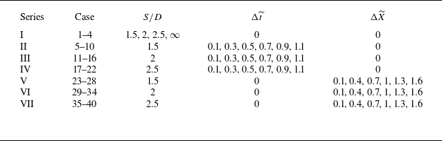
 S/D
 Δt~
 ΔX~
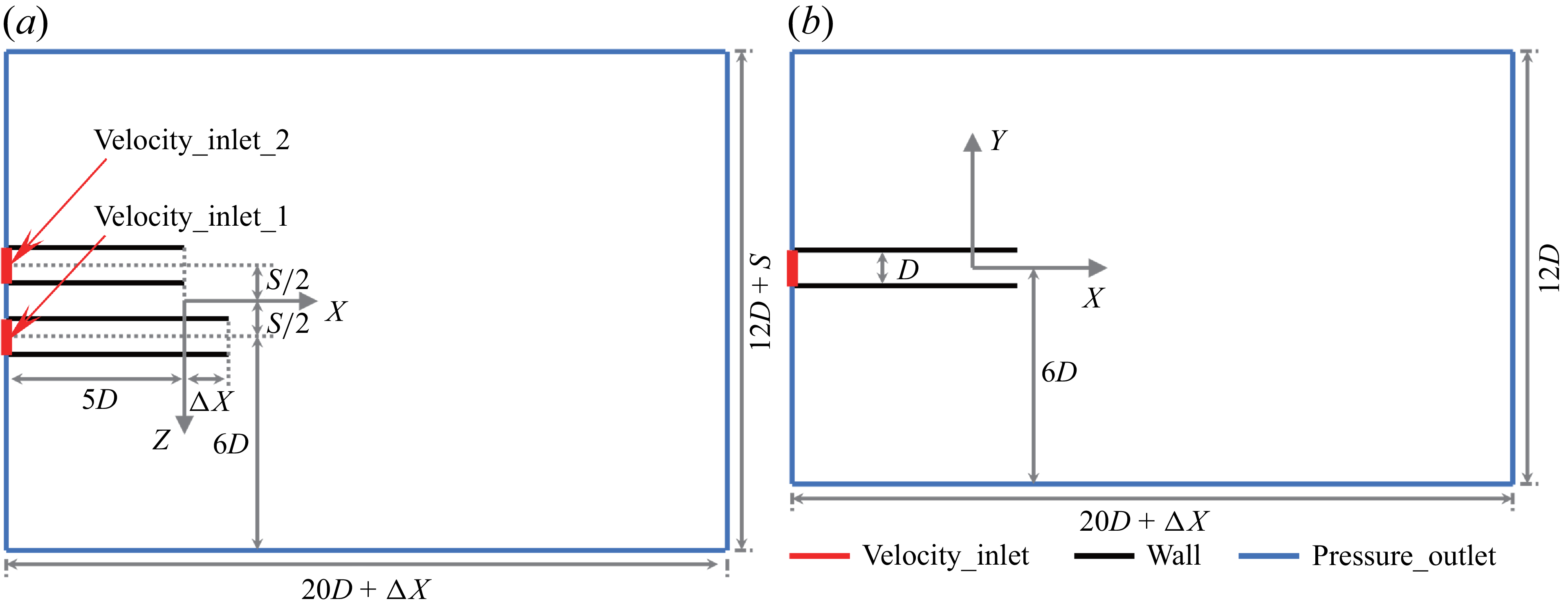
 D
 X−Z
 X−Y
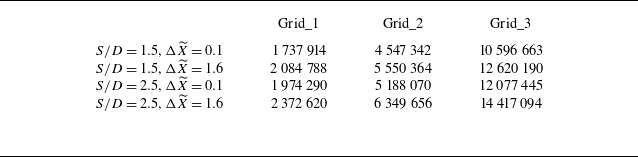
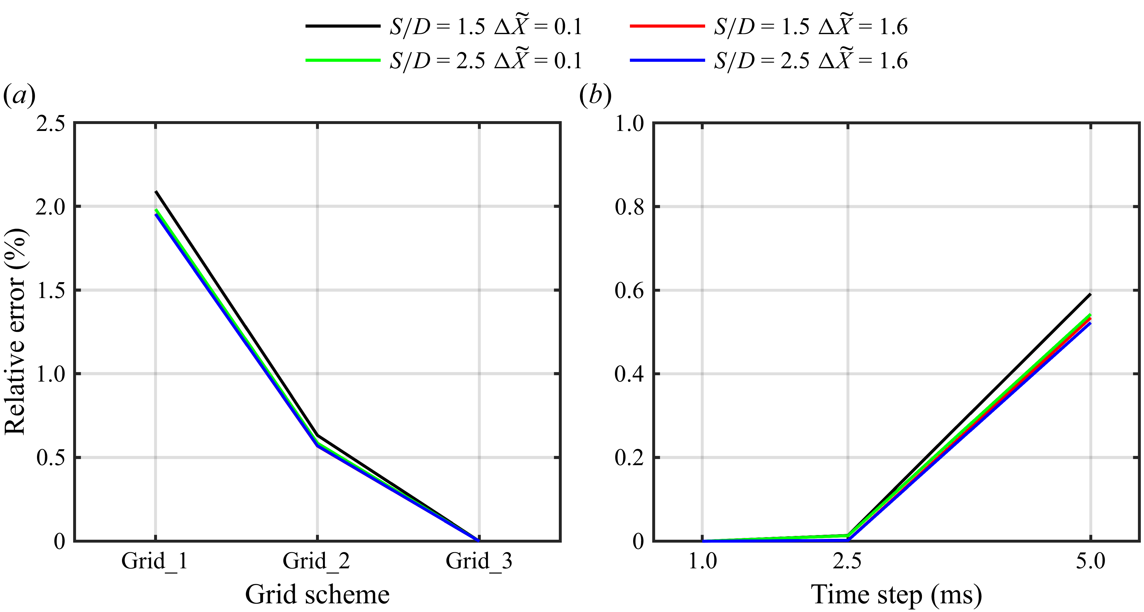
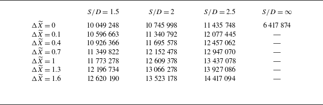
 S/D
 ΔX~

 Q
 S
 Y
 ωY
 X−Z
 S/D=2
 Δt~=0.3
 Um_1st
 Um_2nd

 ΔXc
 ΔRc
 X−Z
 ΔXc
 ΔRc
 S/D=2
 Δt~

 S
 Y
 X−Z
 S/D=1.5
 Δt~=0.3

 ΔF1st(t)
 ΔF2nd(t)
 Δt~
 S/D=1.5

 ΔF¯
 Ffluc
 Δt~
 S/D

 FL_net(t)
 FL_1st(t)
 FL_2nd(t)
 Δt~
 S/D=1.5
 |FL_net|¯
 Δt~
 S/D

 S
 Y
 X−Z
 S/D=2
 ΔX~=0.4
 Δt~=0

 ΔXc
 ΔRc
 X−Z
 ΔX~
 S/D=2

 ΔF1st(t)
 ΔF2nd(t)
 ΔX~
 S/D=1.5

 X−Z
 S/D=1.5
 ΔX~=0.4
 t∗=0.938
 t∗=1.938
 ΔF1st(t)

 ΔF1st(t)
 ΔX~
 S/D
 S1/D
 S/D
 ΔX~

 ΔF¯
 Ffluc
 ΔX~
 S/D

 ΔF¯
 Ffluc
 S1/D
 ΔX~
 S/D

 FL_net(t)
 FL_1st(t)
 FL_2nd(t)
 ΔX~
 S/D=1.5
 |FL_net|¯
 ΔX~
 S/D

 S3
 Δt~>0
 ΔX~>0

 Xc
 Δt~

 ΔF¯
 S3/D

 ΔF¯
 S3/D
 Δt~
 ΔX~
 UmaxT/D=3



