








1 Introduction
A cornerstone of modern ergodic theory is the Birkhoff ergodic theorem, which asserts that for an ergodic transformation T and an integrable observable
$f,$
 the time averages converge almost surely to the spatial average. More precisely,

where

A natural question is what happens for a non-negative observable f that is not integrable. One expects
$S_N(f)$
 to grow faster than linearly, that is, faster than a constant multiple of N. Nevertheless, one might hope that, after renormalization by a suitable sequence
$d_N \to \infty $
 , pointwise convergence still holds. However, Aaronson [Reference AaronsonAar77] showed that such convergence to a non-trivial limit is impossible: for any non-negative
$f\notin L^1$
 and any positive normalizing sequence
$d_N$
 ,

A heuristic explanation comes from order statistics: in the non-integrable case, the largest few terms typically dominate
$S_N(f)$
 . Even a small shift in the position of an extreme value can therefore drastically change the sum, accounting for the oscillations in (1). This motivates the study of trimmed sums, where the largest terms are removed. For
$N \geq 1$
 and
$0 \leq k(N) \leq N-1$
 , we define

where
$\{x_1^N,\ldots , x_N^N\}$
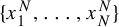 is a reordering of the orbit points
$x, T(x),\ldots , T^{N-1}(x)$
 such that

In the case
$k(N)=0$
 , the sum in (2) is simply the usual Birkhoff sum
$S_N(f)$
 , which we refer to as the untrimmed sum. Trimmed sums originate in classical probability theory, with contributions from Feller [Reference FellerFel68], Kesten [Reference KestenKes93, Reference Kesten and MallerKM92], Mori [Reference MoriMor76, Reference MoriMor77] and others.
To illustrate the concept, consider the function
$f(x)=1/x$
 on the unit interval with a singularity at the origin. The largest values of f occur at the orbit points
$x_1^N,\ldots ,x_{k(N)}^N$
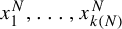 that lie nearest to the origin and the trimmed sum is obtained by summing over the remaining points. However, this example also reveals a key conceptual nuance: if f is not monotonic, even when its only singularity remains at the origin, the points
$x_1^N,\ldots ,x_{k(N)}^N$
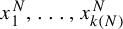 need not be those closest to the singularity. This subtlety will play an important role in the subsequent analysis and we revisit it in §3.1.
We begin by establishing a trimmed strong law of large numbers (SLLN): we seek sequences
$d_N$
 and
$k(N)$
 such that

The case where
$k(N)=K>0$
 is constant is referred to as light trimming, while
$k(N) \to \infty $
 with
$k(N) = o(N)$
 is called intermediate trimming. Trimming a positive fraction of terms, that is,
$k(N)/N \to c>0$
 as
$N \to \infty $
 , is uninteresting from our perspective, since it merely amounts to truncating f, reducing the problem to the classical SLLN.
In the most general sense, a trimmed SLLN always holds: for any non-negative f, there exist sequences
$d_N$
 and
$k(N)$
 such that (3) is satisfied (see [Reference Auer and SchindlerAS25]). While conceptually important, this result is of limited practical use, since it provides no control over the choice of
$d_N$
 or, more crucially,
$k(N)$
 . We therefore focus on functions with polynomial singularities, informally satisfying

A broader definition appears in Definition 2. The functions f are characterized by a singularity order
$\beta>0,$
 with
$\alpha = \beta /d,$
 where d is the manifold dimension. For example, on
$[0,1]$
 , consider
$f(x) = x^{-\alpha }.$

We briefly recall the corresponding independent and identically distributed (i.i.d.) theory, which serves as the probabilistic model for our results for exponentially mixing systems. A detailed account of related results can be found in [Reference Kesseböhmer and SchindlerKS19]. Let
$\{X_N\}_{N \geq 1}$
 be a sequence of non-negative i.i.d. random variables satisfying

For
$k \geq 1$
 , let
$X_N^{(k)}$
 denote the kth largest value among
$X_1, \ldots , X_N$
 . For
$0 \le k(N) \le N-1$
 , set

The classical results for such trimmed sums are as follows.
-
• If $\alpha = 1$
 , then (5) $$ \begin{align} \lim_{N\to\infty}\frac{S_N^K}{N\log N}=1 \quad\text{almost surely}. \end{align} $$This lightly trimmed strong law with a fixed number $K>0$
of trimmed terms was established by Mori [Reference MoriMor77], with related results on trimmed sums and order statistics obtained by Mori [Reference MoriMor76] and Kesten and Maller [Reference Kesten and MallerKM92, Reference Kesten and MallerKM95].
-
• If $\alpha>1$
, then (6) $$ \begin{align} \lim_{N\to\infty} \frac{S_N^{k(N)}}{N^{\alpha} k(N)^{1-\alpha}} = \frac{1}{\alpha - 1} \quad\text{almost surely}. \end{align} $$This strong law holds provided that $k(N)/\log \log N \to \infty $
, as follows from the law of the iterated logarithm of Haeusler and Mason [Reference Haeusler and MasonHM87]. In contrast, if
$k(N)/\log \log N \to c$
for some
$c\in (0,\infty )$
, then (6) fails, by the non-standard law of the iterated logarithm proved by Haeusler [Reference HaeuslerHae93].





Beyond regular variation, Csörgő and Simons [Reference Csörgő and SimonsCS96] obtained corresponding strong law results under intermediate trimming for tails satisfying sandwich-type regular variation, including St. Petersburg-type distributions as a notable special case.
It is widely expected that (5) and (6) extend to sufficiently well-behaved dynamical systems. Indeed, the following dynamical counterparts are known under the renormalization for which (4) holds.
-
• If $\alpha = 1$
, then a dynamical analogue of (5) has been established for
$\psi $
-mixing sequences [Reference Aaronson and NakadaAN03], and in the Gauss map setting, by Diamond and Vaaler [Reference Diamond and VaalerDV86] for the continued-fraction observable
$f(x)=1/x$
. For the same observable over the doubling map, Schindler [Reference SchindlerSch18] showed that light trimming fails, whereas the same law holds after removing approximately
$C\log \log \log N$
largest terms for
$C>1/\log 2$
. Light trimming fails because of the clustering of large values near the singularity at
$0$
, which is a fixed point of the doubling map, so removing finitely many largest terms still leaves substantial residual contributions, a mechanism already reflected by Haynes [Reference HaynesHay14, Theorem 4]. -
• If $\alpha> 1$
, then [Reference Kesseböhmer and SchindlerKS19] showed a dynamical analogue of (6) for systems with a spectral gap on a suitable Banach space and observables whose truncations have at most linear growth and whose level-set indicators remain uniformly bounded in the Banach space norm (see also Remark 9). This includes piecewise expanding interval maps with observables whose truncations and level-set indicators have uniformly controlled bounded variation. The result was later extended to subshifts of finite type via a quasi-Hölder framework [Reference Kesseböhmer and SchindlerKS20].






While these results are well established for i.i.d. sequences and certain specific dynamical systems, their validity for general exponentially mixing systems remains an open question. In this paper, we address this gap by establishing trimmed strong laws of large numbers for such systems. For
$\alpha =1$
 , we prove that a dynamical analogue of (5) holds in full. For
$\alpha>1$
 , we prove a dynamical analogue of (6) under the trimming condition
$k(N)/(\log N)^{\epsilon } \to \infty $
 for some
$\epsilon> 0$
 , which is close to the optimal
${k(N)/\log \log N \to \infty }$
 condition known for i.i.d. sequences.
Furthermore, we advance the theory by proving the corresponding distributional limit theorems. Once a trimmed SLLN is established, the natural next question concerns the size of second-order deviations. In this context, an untrimmed analogue arises from the distributional limit theorems of Gnedenko and Kolmogorov [Reference Gnedenko and KolmogorovGK68] for observables not in
$L^2$
 . They show that, in the i.i.d. setting, if f has regularly varying tails, which is similar to our assumption of polynomial singularities, then there are sequences
$a_N$
 and
$b_N$
 such that

for a stable distribution L, where
$\Rightarrow $
 denotes distributional convergence.
Early work on the effect of extreme terms on heavy-tailed sums includes Darling [Reference DarlingDar52] and Arov and Bobrov [Reference Arov and BobrovAB60]. For lightly trimmed sums, Hall [Reference HallHal78] established distributional limits in the stable-domain setting. In particular, for fixed
$K\geq 1$
 , there exist sequences
$a_N$
 and
$b_N$
 such that

where L is a non-degenerate limiting distribution. As shown by Kesten [Reference KestenKes93], the normalizing sequences
$a_N$
 and
$b_N$
 do not depend on K, whereas the limiting distribution L does. Mori [Reference MoriMor84] further developed the distributional theory of lightly trimmed sums, deriving in particular an explicit formula for the limiting distribution L.
The intermediately trimmed case, where
$k(N)\rightarrow \infty $
 but
$k(N)=o(N)$
 , is of special interest because the limiting distribution is always normal. Csörgő et al [Reference Csörgő, Horváth and MasonCHM86] show that, for
$k(N)\rightarrow \infty $
 with
$k(N)=o(N)$
 , there exist sequences
$a_N$
 and
$b_N$
 such that

where
$\mathcal {N}(0,1)$
 is the standard normal distribution with mean
$0$
 and variance
$1$
 . Subsequently, Csörgő et al [Reference Csörgő, Haeusler and MasonCHM88] provided an explicit characterization of the norming sequences
$a_N$
 and
$b_N$
 in this case. Related distributional limits for intermediately trimmed sums normalized by extreme order statistics were obtained by Teugels [Reference TeugelsTeu81].
While most classical results on distributional convergence are formulated for i.i.d. sequences, dynamical systems with strong mixing properties have also been studied in this context. For example, Bazarova et al [Reference Bazarova, Berkes and HorváthBBH16] established asymptotically Gaussian behaviour for trimmed sums of partial quotients under the Gauss map. Our results extend this line of work to exponentially mixing systems of all orders.
In Theorems 12 and 15, we prove dynamical analogues of (7) and (8) for systems that are exponentially mixing of all orders. Establishing these limit theorems in a dependent setting requires handling the interplay between extreme values (governing the trimming) and the system’s correlation structure. We show that the lightly trimmed sum converges to a non-standard distribution described in §3.6, while the intermediately trimmed sum, when suitably normalized, converges to a centred normal distribution. Collectively, these results provide a nearly complete dynamical counterpart to the classical trimming theory for i.i.d. sequences with polynomial tails, extending it to a broad class of non-independent systems.
The remainder of the paper is organized as follows. Section 2 states the main theorems, and §3.1 establishes the asymptotic equivalence between removing the largest observations and excluding points near a critical value. Moment estimates for truncated ergodic sums are given in §3.2. Sections 3.3 and 3.4 prove strong laws of large numbers under light and intermediate trimming, respectively. The tools for the non-standard limit law under light trimming are developed in §§3.5 and 3.6, with the proof completed in §3.7. Section 3.8 summarizes facts on distributional convergence and §3.9 establishes distributional limits under intermediate trimming.
Throughout this paper, we adhere to the following notational conventions.
-
• For real-valued functions $\alpha $
and
$\beta $
defined on
$\mathbb {N}$
or
$\mathbb {R}$
, we write
$\beta = O(\alpha )$
if there exists a constant
$C>0$
such that
$|\beta (x)| \leq C |\alpha (x)|$
for all x and
$\beta =o(\alpha )$
if
$|\beta (x)|/|\alpha (x)| \to 0$
as
$x \to \infty $
. If
$\lim _{x\to \infty } \alpha (x)/\beta (x) = 1$
, we write
$\alpha \sim \beta $
. -
• For $[0,\infty )$
-valued functions
$\alpha $
and
$\beta $
, we often write
$\beta \ll \alpha $
instead of
$\beta =O(\alpha )$
,
$\beta \gg \alpha $
instead of
$\alpha =O(\beta )$
, and
$\beta \asymp \alpha $
if both
$\beta \ll \alpha $
and
$\alpha \ll \beta $
. -
• For a measurable function f, its expectation is denoted $\mathbb {E} f = \int f \, d\mu $
if
$f \in L^1(\mu )$
and its variance by
$\mathrm {Var} f = \mathbb {E}((f-\mathbb {E}f)^2)$
if
$f \in L^2(\mu )$
. -
• For $x^* \in M$
and
$r \ge 0$
, let
$B_r(x^*)$
denote the ball of radius r centred at
$x^*$
. For simplicity, set
$B_r(x^*) = \emptyset $
for
$r < 0$
; the notation
$\mathbf {1}_A$
denotes the indicator function of a measurable set A. -
• For $d \geq 1$
, let
$B_d$
denote the volume of the d-dimensional unit ball.














2 Polynomial singularities
Let M be a compact smooth d-dimensional Riemannian manifold. Fix
$\kappa \geq 1$
 . Let
${T:M\to M}$
 be a
$C^{\kappa }$
 map preserving a probability measure
$\mu $
 that is absolutely continuous with respect to the Riemannian volume
$\mathrm {vol},$
 with a continuous density
$\rho = {\, {d}\mu }/{\, {d}\mathrm {vol}}.$

We assume that the system is exponentially mixing for
$C^\kappa $
 observables, as defined below. When needed, we further assume that it is exponentially mixing of all orders for
$C^\kappa $
 observables.
Definition 1. (Exponential mixing of order m)
The system
$(M,\mathcal {B}(M),\mu ,T)$
 is said to be exponentially mixing of order m if there are constants
$C_m\geq 0$
 and
$\gamma>0$
 such that, for all functions
$f_0,\ldots , f_{m-1} \in C^{\kappa }(M)$
 and integers
$0 \leq k_0 \leq \cdots \leq k_{m-1}$
 , we have

In particular, when
$m = 2$
 , the system is said to be exponentially mixing. If (9) holds for all
$m \geq 2,$
 the system is called exponentially mixing of all orders.
Since m is fixed or ranges over a bounded set in each application below, the dependence of
$C_m$
 on m is immaterial and we simply write C in place of
$C_m$
 in (9).
Definition 2. Let
$x^* \in M$
 and let
$f\in C^{\kappa }(M\setminus \{x^*\})$
 be a non-negative measurable function. We say that f has a power singularity of order
$\mathrm {Ord}_{x^*}(f)=\beta $
 at
$x^*$
 if the function defined by

admits a
$C^{\kappa }$
 extension in a neighbourhood of
$x^*$
 and satisfies
$g(x^*)>0$
 , where
$d(\cdot , \cdot )$
 denotes the geodesic distance on M. In this case, we call
$g(x^*) = \mathrm {Res}_{x^*}(f)$
 the residue of f at
$x^*$
 .
Remark 3. The function
$f(x)=x^{-\alpha }$
 on
$[0,1]$
 does not strictly satisfy Definition 2, since the singularity at
$x^*=0$
 is one-sided. On
$\mathbb {T}^1$
 , it would be two-sided. Nevertheless, the limit theorems below still apply after replacing
$B_1$
 by
$B_1/2=1$
 . Indeed,
$\mathrm {vol}(f>t)=t^{-1/\alpha },$
 whereas for a proper power singularity h of order
$\alpha $
 ,

Since
$B_1=2$
 corresponds to the two-sided case on
$\mathbb {T}^1$
 , the one-sided setting contributes half this constant. This accounts for the factor
$1/2$
 difference between the constants in the i.i.d. cases (5), (6) and those in Theorems 5 and 8.
Under this condition, for
$r>0$
 , there exists
$\epsilon (r)>0$
 such that

whenever
$d(x,x^*)\leq r,$
 and
$\epsilon (r)\rightarrow 0$
 as
$r\rightarrow 0$
 . Without loss of generality, we assume that
$\epsilon $
 is
$C^{\kappa }$
 smooth and monotonically decreasing as r approaches
$0$
 . In the proofs, we will always take
$r = r_N$
 with
$r_N \to 0$
 as
$N \to \infty $
 , for example,
$r_N =({(\log \log N)^6}/({N \log N}))^{{1}/{d}}$
 in §3.3 and
$r_N\sim ({k(N)}/({B_d \rho (x^*) N}))^{{1}/{d}}$
 in §3.4.
Furthermore, let
$C_0> 0$
 be a constant such that

We will also often denote
$\alpha ={\beta }/{d}$
 .
Definition 4. (Slowly recurrent point)
A point
$x^*\in M$
 is called slowly recurrent if, for every
$A, C>0$
 , there exists
$r_0>0$
 such that for all
$0<r<r_0$
 and positive integers
${n\leq C |\!\log r|}$
 , it holds that

This notion of slow recurrence is closely related to the mixing properties of the system. Specifically, if the system
$(M, \mathcal {B}(M),\mu ,T)$
 is exponentially mixing, then
$\mu $
 -almost every point is slowly recurrent (see [Reference Dolgopyat, Fayad and LiuDFL22, Lemma 4.14]).
Throughout the rest of the paper, we assume that
$x^*$
 is the unique singularity of f, that it is of the power type described in Definition 2 and that
$\rho (x^*)>0$
 . Furthermore, we assume that
$x^*$
 is slowly recurrent as defined in Definition 4.
We will establish trimmed limit theorems for functions that exhibit non-integrable power singularities.
Theorem 5. Assume that the system
$(M, \mathcal {B}(M), \mu , T)$
 is exponentially mixing. Let
${f \in C^{\kappa }(M \setminus \{x^*\})}$
 be a function with a power singularity of order
$\operatorname {Ord}_{x^*}(f)=d$
 at a slowly recurrent point
$x^*\in M$
 . Then, for every fixed
$K \geq 1$
 ,

Remark 6. For the doubling map on
$\mathbb T^1$
 , Theorem 5 cannot be applied directly to the observable

because
$f_c$
 is not
$C^\kappa $
 at the identified endpoint
$0=1$
 , where
$\kappa \geq 1$
 is the regularity exponent fixed at the beginning of this section. It does, however, apply to
$\hat f_c=f_c+\psi _c$
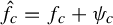 , where
$\psi _c$
 is a bounded function, vanishing near c, chosen so that
$\hat f_c$
 is non-negative and
$C^\kappa $
 away from the singularity at c. Since adding a bounded function does not affect the lightly trimmed strong law, we obtain a lightly trimmed strong law for
$f_c$
 and Lebesgue-almost every
$c\in [0,1]$
 , because almost every point is slowly recurrent. In contrast, for the observable
$f(x)=1/x$
 , no lightly trimmed strong law holds [Reference HaynesHay14], although an intermediately trimmed strong law does hold [Reference SchindlerSch18]. Hence, while light trimming fails to yield a strong law for
$1/x$
 , it does yield one for
$1/|x-c|$
 for Lebesgue-almost every
$c\in [0,1]$
 .
This example also shows that the regularity of the observable away from the singularity is not restrictive: provided that the required
$C^\kappa $
 structure holds near the singularity, bounded irregularities away from the singularity can be removed by adding a bounded function supported away from it.
A lightly trimmed strong law implies an untrimmed weak law. In the i.i.d. setting, this follows immediately from Kesten’s results [Reference KestenKes93]. In the ergodic setting, the implication follows provided that f takes values comparable to the leading order of the trimmed sum only with probability
$o(1/N)$
 ; see [Reference Auer and SchindlerAS25, Remark 7]. The corresponding result in our setting is the following corollary.
Corollary 7. (Convergence in probability)
Under the assumptions of Theorem 5, we have

Theorem 8. Assume that the system
$(M, \mathcal {B}(M), \mu , T)$
 is exponentially mixing of all orders. Let
$f \in C^{\kappa }(M \setminus \{x^*\})$
 be a function with a power singularity of order
$\operatorname {Ord}_{x^*}(f)=\beta>d$
 at a slowly recurrent point
$x^*\in M$
 . Suppose that
$k:\mathbb {N}\to \mathbb {N}$
 is non-decreasing,
$k(N)=o(N)$
 and there exists
$\epsilon>0$
 such that
$\lim _{N\rightarrow \infty } {k(N)}/{(\log N)^{\epsilon }} = \infty .$
 Then, it holds that

where
$\alpha ={\beta }/{d}$
 .
Remark 9. The assumption of exponential mixing of all orders is used here as an abstract quantitative mixing condition. It can be established by several mechanisms. In standard expanding and hyperbolic settings, it often follows from spectral estimates for transfer operators on appropriate function spaces, together with suitable multiplication estimates. Examples include uniformly expanding maps, piecewise expanding maps and volume-preserving Anosov diffeomorphisms [Reference BowenBow08, Reference VianaVia97]. Alternatively, [Reference Dolgopyat, Fayad and LiuDFL22, Theorem A.3] derives exponential mixing of all orders from quantitative equidistribution along unstable leaves and applies, among other examples, to time-one maps of contact Anosov flows, mostly contracting systems, partially hyperbolic translations on homogeneous spaces and partially hyperbolic automorphisms of nilmanifolds. Products and certain skew products are also treated in [Reference Dolgopyat, Fayad and LiuDFL22]. Thus, Theorem 8 uses only the multiple-correlation estimates stated above, independently of the mechanism by which they are obtained. It remains open whether ordinary exponential mixing implies exponential mixing of all orders [Reference Dolgopyat, Kanigowski and Rodriguez HertzDKRH24, Question 1.7].
This distinction is relevant because, even when a spectral gap is available, existing intermediately trimmed SLLNs apply only to restricted classes of observables. In [Reference Kesseböhmer and SchindlerKS19], the relevant condition, called property
$\mathfrak {D}$
 , includes in particular the growth condition

The issue is not the possible loss of smoothness under truncation, which can be handled by smooth approximation, but the growth of the norm after truncation. In derivative-based norms, such as
$C^\kappa $
 norms or the smooth anisotropic spaces of Gouëzel and Liverani [Reference Gouëzel and LiveraniGL06], truncation near singularities may yield superlinear growth. For instance,
${f(x)=1/x}$
 truncated at height n has
$C^1$
 norm of order
$n^2$
 . Thus, the above linear bound is natural in low-regularity spaces such as the space of functions of bounded variation, but generally fails in the smooth function spaces used for uniformly hyperbolic systems. Consequently, the observables covered by [Reference Kesseböhmer and SchindlerKS19] are typically not available in these settings.
Remark 10. For i.i.d. observations, as discussed in §1, a stronger statement holds: a trimmed SLLN applies whenever
$k(N)=o(N)$
 and

The same condition should be attainable for Theorem 8 if one could establish Bernstein-type moderate deviation estimates for the shrinking-target counts
$S_N({\mathbf {1}}_{B_{r_N}(x^*)})$
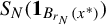 and for the truncated sums
$S_N(f \cdot (1-{\mathbf {1}}_{B_{r_N}(x^*)}))$
 . However, under our current assumption of exponential mixing of all orders, such estimates appear to lie beyond the reach of the moment method employed here. Moreover, it is not clear that they can be deduced from the mixing assumption alone, since quantitative mixing does not in general imply Bernstein-type inequalities of i.i.d. strength. Indeed, Adamczak [Reference AdamczakAda08, §3.3] constructs a Markov chain for which no uniform Bernstein inequality with an i.i.d.-optimal large-deviation term can hold over all bounded centred observables. One can verify that this chain is exponentially
$\beta $
 -mixing. Since exponential
$\beta $
 -mixing implies exponential mixing of every finite order for bounded coordinate observables, this suggests that exponential multiple mixing alone is insufficient to guarantee concentration inequalities of i.i.d. strength. We therefore restrict ourselves to the present formulation of the theorem and leave this strengthening for future work.
Remark 11. Analogously, one can derive intermediate trimming for the case
${\operatorname {Ord}_{x^*}(f) = d}$
 . The corresponding statement is as follows: if
$k(N) \rightarrow \infty $
 and
$k(N)=o(N)$
 , then

However, given that Theorem 5 already establishes the strong law under light trimming, in what can be regarded as its strongest form with
$K=1,$
 the result (12) is not the most interesting one. We therefore omit the proof and leave it as an exercise for the interested reader.
It should be noted, however, that (12) does not follow from the seemingly stronger light trimming result in Theorem 5. Indeed, as shown in [Reference Auer and SchindlerAS25], there exist functions for which trimming is not stable under removal of additional terms: an SLLN may hold for some trimming sequence
$k(N)$
 , but fail if more terms are removed, say
$k'(N)> k(N)$
 .
Theorem 12. Assume that the system
$(M, \mathcal {B}(M), \mu , T)$
 is exponentially mixing of all orders. Let
$f \in C^{\kappa }(M \setminus \{x^*\})$
 be a function with a power singularity of order
$\operatorname {Ord}_{x^*}(f)=\beta>({d}/{2})$
 at a slowly recurrent point
$x^*\in M$
 . Then, for every fixed
$K\geq 0$
 , there exist constants
$a_N$
 and a non-degenerate distribution Y such that

where
$\alpha ={\beta }/{d}$
 . Furthermore, it holds that

Remark 13. As noted in §1, the normalizing sequences
$a_N$
 and
$N^\alpha $
 do not depend on the trimming number K, similarly to the i.i.d. case studied by Kesten [Reference KestenKes93]. The limit Y, however, does depend on K. More specifically, Y is the light-trimming limit generated by the limiting Poisson process of rare visits to the singularity
$x^*$
 , as described precisely in Proposition 38.
This is the same limiting mechanism that appears in the classical i.i.d. light-trimming theory in the stable-domain setting studied by Hall [Reference HallHal78]. In particular, the limiting distribution Y coincides with that obtained in the i.i.d. case with the same marginal distribution. In the present setting, the Poisson process description yields the corresponding light-trimming limit, with the scale determined by the local tail asymptotics of f near
$x^*$
 .
Remark 14. The case
$K=0$
 corresponds to the untrimmed setting, where stable limit laws are expected. Although this is likely well known and can be derived by combining the Poisson limit theorem from [Reference Dolgopyat, Fayad and LiuDFL22] with the approach of Tyran-Kamińska [Reference Tyran-KamińskaTyr10], we include it in the statement for completeness.
Theorem 15. Assume that the system
$(M, \mathcal {B}(M), \mu , T)$
 is exponentially mixing of all orders. Let
$f \in C^{\kappa }(M \setminus \{x^*\})$
 be a function with a power singularity of order
${\operatorname {Ord}_{x^*}(f)=\beta>({d}/{2})}$
 at a slowly recurrent point
$x^*\in M$
 . Suppose
$k(N)$
 is a function with
$k(N)\rightarrow \infty $
 as
$N\rightarrow \infty $
 and
$k(N)=o(N).$
 Then, there exist constants
$a_N$
 such that

where
$\alpha ={\beta }/{d}$
 and

Furthermore, the normalizing constants
$a_N$
 satisfy

3 Proofs
3.1 Large observations and closest points
Let us revisit an issue mentioned in §1: the conceptual relationship between trimming based on extremal function values and trimming based on geometric proximity to a singularity. For the canonical radial example
$f(x)=1/\|x\|$
 ,
$x=(x_1,x_2)\in B_1(0)\setminus \{0\}\subset \mathbb R^2,$
 ordering by function value is equivalent to ordering by distance from the singularity. This equivalence fails in general. Indeed, for
$f_\delta (x)=(1+\delta x_1)/\|x\|$
 with
$0<\delta <1$
 , the normalized singularity profile
$g_\delta (x)=f_\delta (x)\|x\|=1+\delta x_1$
 extends smoothly across the origin, yet there exist points arbitrarily close to the origin whose ordering by distance is opposite to their ordering by function value. For instance, for
$p_r=(-r,0)$
 and
$q_r=(r+\delta r^2,0)$
 , with
$r>0$
 sufficiently small, one has
$d(p_r,0)<d(q_r,0)$
 but
$f_\delta (p_r)<f_\delta (q_r).$

Despite this potential discrepancy, the asymptotic behaviour often remains similar. We prove that the trimmed sum is asymptotically equivalent to the sum obtained by removing points closest to the singularity, allowing us to work with this geometric notion of trimming in the proofs that follow.
Consider k as either a constant K or a function
$k(N)$
 . Let
$\hat {S}_N^k(f)(x)$
 denote the sum obtained by removing the k closest visits to
$x^*$
 , formally defined as

where
$\hat {x}_l$
 is the lth closest point to
$x^*$
 among
$\{x,\ldots ,T^{N-1}(x)\}$
 . By definition of
$S_N^k,$
 it clearly holds that

However, let
$x_1,\ldots ,x_k$
 be the points that maximize f among
$\{x,\ldots ,T^{N-1}(x)\},$
 ordered by increasing distance to
$x^*$
 so that

Then, we have

If
$\{x_1,\ldots ,x_k\}=\{\hat {x}_1,\ldots ,\hat {x}_k\}$
 , then the sums coincide. Otherwise, let
$1\leq m\leq k$
 be the number of points
$x_i$
 not in
$\{\hat {x}_1,\ldots ,\hat {x}_k\}$
 . Since x is almost surely not eventually periodic, no two points in the orbit of such an x coincide. Therefore, there are also exactly m points among the
$\hat {x}_i$
 not contained in
$\{x_1,\ldots ,x_k\}$
 . Relabel these points so that
$\{y_1,\ldots ,y_m\}=\{x_1,\ldots ,x_k\}\setminus \{\hat {x}_1,\ldots ,\hat {x}_k\},$
 and likewise for
$\{\hat {y}_1,\ldots ,\hat {y}_m\}$
 , keeping the original order, although the order itself is not essential for the subsequent argument.
For any
$i,j\in \{1,\ldots ,m\}$
 , by construction, we have
$f(y_i)\geq f(\hat {y}_j)$
 since
$y_i$
 was chosen among the largest values. However, by (10), we have

At the same time,
$\sum _{i=1}^m f(\hat {y}_i)\leq S_N^k(f)(x)$
 and, therefore,

and we conclude

Lemma 16. Let
$k(N)=o(N),$
 and suppose that f has a power singularity at
$x^*$
 . Then, for almost every
$x,$
 it holds that

Proof. Let G be the set of points
$x\in M$
 satisfying

By the ergodic theorem,
$\mu (G)=1$
 . For
$x\in G$
 and
$\varepsilon>0$
 , choose l sufficiently large so that
$2^{-l} < \varepsilon $
 , then for all sufficiently large N, it follows that

This implies that all
$k(N)$
 closest points
$\hat {x}_1,\ldots ,\hat {x}_{k(N)}$
 lie in
$B_{2^{-l}}(x^*)$
 , so
$d(\hat {x}_{k(N)},x^*) \leq 2^{-l}$
 .
Lemma 17. Let
$k(N)=o(N)$
 and suppose f has a power singularity at
$x^*$
 . Then, for almost every
$x,$


Proof. Applying the same argument as in Lemma 16 to the sets
$\{f>R\}$
 , where
$R>0$
 , instead of balls, yields that almost surely,
$f(x_{k(N)})\rightarrow \infty $
 as
$N\rightarrow \infty $
 . Keeping in mind that
$f(y) \leq C_0 d(x^*,y)^{-\beta }$
 for all points y, the claim follows.
Lemma 18. Let
$k(N)=o(N)$
 and suppose that f has a power singularity at
$x^*$
 . Then,

for almost every
$x.$

Proof. By definition,
$d(x^*,\hat {x}_{k(N)}) \leq d(x^*,x_{k(N)})$
 , so it suffices to show

If
$d(x^*,\hat {x}_{k(N)})\ge d(x^*,x_{k(N)}),$
 there is nothing to prove. Otherwise,
$x_{k(N)}\notin \{\hat {x}_1,\ldots , \hat {x}_{k(N)}\}$
 and, hence, there exists some
$1\leq i\leq k(N)$
 such that
$\hat {x}_i\notin \{x_1,\ldots ,x_{k(N)}\}.$
 By the definition of
$x_1,\ldots ,x_{k(N)}$
 , we have
$f(\hat {x}_i)\leq f(x_{k(N)}).$
 Moreover,
$d(x^*,\hat {x}_i)\leq d(x^*,\hat {x}_{k(N)}).$
 Thus, for all sufficiently large N,

Since
$d(x^*,\hat {x}_{k(N)})\to 0$
 and
$d(x^*,x_{k(N)})\to 0$
 as
$N\to \infty $
 , we have

and, hence, (16) follows.
Lemma 19. Let
$k(N)=o(N)$
 and suppose f has a power singularity at
$x^*$
 . Then, it holds that

Proof. Since
$\hat {S}_N^{k(N)}(f) \geq S_N^{k(N)}(f)$
 by definition, it suffices to show that

Given that
$d(x^*,\hat {x}_{k(N)}),\, d(x^*,x_{k(N)}) \rightarrow 0$
 as
$N\to \infty ,$
 the desired inequality follows directly from (14).
3.2 Moments of truncated observables
In this section, we collect the estimates on truncated observables that will be used in the proofs of the main theorems. Throughout, f is assumed to possess a power singularity of order
$\beta $
 at a slowly recurrent point
$x^*$
 . The basic truncations are obtained by removing a small ball around the singularity: for
$\epsilon>0$
 , we call

a truncation of f. The guiding idea is that, once the largest observations are removed, the trimmed ergodic sum can be compared with an ordinary ergodic sum of a suitable truncation of f. We therefore require two quantitative ingredients: control of short returns to small balls around
$x^*$
 and moment estimates for ergodic sums of functions truncated near
$x^*$
 .
We begin with a standard consequence of exponential mixing, which will be used to control correlations of small balls.
Lemma 20. (Mixing estimate for balls)
If the system
$(M, \mathcal {B}(M), \mu , T)$
 is exponentially mixing as defined in (9), then for any balls
$B_1, B_2 \subset M$
 and any
$k \in \mathbb {N}$
 , we have

Lemma 20 is a standard consequence of exponential mixing and its proof is therefore omitted.
For the later arguments, it is convenient to formulate the truncation estimates slightly more generally. Instead of only removing balls
$B_\epsilon (x^*)$
 , we will allow the removed sets to be small perturbations of balls. This flexibility is useful because the relevant truncation levels will depend on N and, in some places, the natural sets are not exactly balls but are asymptotically equivalent to balls around
$x^*$
 .
We shall say that a sequence of sets
$A_N\subset M$
 is regularly adapted if there exists a sequence
$r_N\to 0$
 and constants
$a,a'\ge 0$
 such that the following two conditions hold.
-
(R1) There exists a sequence $\delta _N=o(r_N)$
such that (17) $$ \begin{align} B_{r_N}(x^*) \subset A_N \subset B_{r_N+\delta_N}(x^*)\quad \text{for all } N\ge1. \end{align} $$
-
(R2) For every sequence $\epsilon _N=o(r_N)$
, there are approximating functions
$h_N\in C^\kappa (M)$
such that
${\mathbf {1}}_{A_N}\le h_N\le 1$
, and (18) $$ \begin{align} \|{\mathbf{1}}_{A_N}-h_N\|_{L^1} \ll \epsilon_N r_N^a \quad \text{and} \quad \|h_N\|_{C^{\kappa}} \ll \epsilon_N^{-\kappa} r_N^{-a'}. \end{align} $$





Remark 21. The parameter
$r_N$
 should be viewed as the effective radius of
$A_N$
 . This scale is well defined asymptotically: if two sequences
$r_N$
 and
$r_N'$
 both satisfy (17) for the same sets
$A_N$
 , then
$r_N\sim r_N'$
 . Hence, all asymptotic estimates below are independent of the particular admissible choice of
$r_N$
 .
The next two elementary observations record the consequences of regular adaptation that will be used throughout the rest of the section.
Lemma 22. Let
$A_N\subset M$
 be a sequence of sets that is regularly adapted. Then,

Proof. By (17),
$B_{r_N}(x^*)\subset A_N\subset B_{r_N+\delta _N}(x^*)$
 and
$\delta _N=o(r_N).$
 Since
$\mu (B_r(x^*))\sim B_d\rho (x^*)r^d$
 and
$r_N+\delta _N\sim r_N$
 , the conclusion follows by squeezing.
Lemma 23. Let
$A_N\subset M$
 be a sequence of sets that is regularly adapted. Then, for all constants
$A,\,C>0$
 , there exists
$N_0>1$
 such that for all
$N>N_0$
 and all positive integers
$1\le n\le C|\!\log r_N|$
 , one has

Proof. Let
$\widetilde r_N = r_N + \delta _N$
 . By (17),
$A_N \subset B_{\widetilde r_N}(x^*)$
 and
$\widetilde r_N \sim r_N$
 . Hence,
$|\!\log \widetilde r_N| \sim |\!\log r_N|$
 and for large N,
$1\le n \le C|\!\log r_N|$
 implies
$1\le n \le 2C|\!\log \widetilde r_N|$
 . Applying the slow recurrence with exponent
$A+2$
 and time constant
$2C$
 yields

Since
$\widetilde r_N \sim r_N$
 and
$\mu (B_{\widetilde r_N}(x^*)) \sim B_d\,\rho (x^*)\,\widetilde r_N^{\,d}$
 , the right-hand side is bounded by
$r_N^d|\!\log r_N|^{-A}$
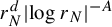 for all sufficiently large N. The result follows from the inclusion
$A_N \cap T^{-n}(A_N) \subset B_{\widetilde r_N}(x^*) \cap T^{-n}B_{\widetilde r_N}(x^*)$
 .
For a sequence of sets
$A_N$
 that is regularly adapted, we refer to
$f\cdot (1-{\mathbf {1}}_{A_N})$
 as a generalized truncation of f. We next prove a short-time covariance estimate for such truncations.
Lemma 24. (Covariance for the generalized truncation)
Let
$\beta>({d}/{2})$
 , let
$A_N \subset M$
 be regularly adapted and set
$f_N=f \cdot (1-{\mathbf {1}}_{A_N}).$
 Then, for any constants
$A,\,C>0$
 , there exists
$N_0>1$
 such that for all
$N>N_0$
 and positive integers
$1\leq n\leq C |\!\log r_N|$
 ,

Proof. We first record a local moment bound. Since
$f(x) \le C_0\,d(x,x^*)^{- \beta }$
 and
$\rho $
 is continuous, for any
$s>0$
 with
$s\beta>d$
 , there exists a constant
$K_s$
 independent of r, such that for all sufficiently small
$r>0$
 ,

In addition, for small enough
$r>0$
 , it holds that

Choose
$q>1$
 such that
$q^2\beta>d$
 and
$\beta -d+({d}/{q^2})>0$
 . Denote by p the conjugate exponent of q, and choose
$H>0$
 so large that
$H(\beta -d+({d}/{q^2}))\ge A+2$
 and
$H(2\beta -d)\ge A+2$
 .
Set
$\hat {r}_N=r_N|\!\log r_N|^H$
 and define
$\hat {f}_N=f_N \cdot (1-{\mathbf {1}}_{B_{\hat {r}_N}(x^*)}).$
 For
$1\leq n <C |\!\log r_N|,$
 we decompose the term
$\mathbb {E}(f_N \cdot f_N\circ T^n)$
 as

where

Bounding
$\mathfrak {A}, \mathfrak {B}$
 : applying Hölder’s inequality twice with exponents p and q yields

Note that always
$pq \geq 4$
 ; hence,
$p q \beta> d$
 . Since
$\hat {f}_N$
 vanishes on
$B_{\hat r_N}(x^*)$
 and
$f_N$
 vanishes on
$A_N\supset B_{r_N}(x^*)$
 , we can apply (20) to obtain

For sufficiently large N, it follows that

The same estimate applies to
$\mathfrak {B}.$

Bounding
$\mathfrak {C}$
 : we apply the Cauchy–Schwarz inequality and obtain

for N sufficiently large.
Bounding
$\mathfrak {D}$
 : let
$A'>0$
 be fixed, to be chosen later. By the slow recurrence property (see Definition 4), for N sufficiently large, for
$1\le n<2C|\!\log \hat {r}_N|$
 , it holds that

Applying Hölder’s inequality and (20), we obtain

Note that
$|\!\log \hat {r}_N|{\kern-1pt}\ge{\kern-1pt} \tfrac 12 |\!\log r_N|$
 for sufficiently large N and choosing
${A'{\kern-1pt}>{\kern-1pt}Hd{\kern-1pt}+{\kern-1pt}p(A{\kern-1pt}+{\kern-1pt}2)}$
 gives

Combining the bounds for
$\mathfrak {A}$
 ,
$\mathfrak {B}$
 ,
$\mathfrak {C}$
 and
$\mathfrak {D}$
 , we obtain

where

Choose
$N_0$
 sufficiently large so that
$\tilde {K}|\!\log r_N|^{-2}\le 1$
 for all
$N>N_0$
 . Then,

which completes the proof.
Proposition 25. Fix
$m_1,m_2\in \mathbb {N} \cup \{0\}$
 , and set
$m=m_1+m_2.$
 Assume that
$m\geq 2$
 and that the system is exponentially mixing of order m.
Suppose that
$\mathrm {Ord}_{x^*}(f)=\beta>({d}/{2})$
 . Let
$A_N\subset M$
 be a sequence of sets that is regularly adapted and satisfies
$N r_N^{d} \rightarrow \infty $
 . Define
$f_N=f \cdot (1-{\mathbf {1}}_{A_N}).$
 Then,

where
$\alpha ={\beta }/{d}$
 ,

and

The cases
$m=0$
 and
$m=1$
 are trivial. Indeed, if
$m=0$
 , then both sides of (21) are equal to
$1$
 . If
$m=1$
 , then either
$(m_1,m_2)=(1,0)$
 or
$(0,1)$
 , and the corresponding moment in (21) vanishes by centring. Thus, as an immediate consequence of Proposition 25 and the method of moments, we obtain the following joint distributional limit. This consequence will be used in §3.9, while the explicit moment estimate of Proposition 25 will also be needed later.
Corollary 26. Assume that the system is exponentially mixing of all orders and that the remaining assumptions of Proposition 25 hold. Then,

as
$N\to \infty ,$
 where the right-hand side denotes a vector of independent normal random variables and
$\sigma ^2={1}/({2\alpha -1}).$

Proof of Proposition 25.
Denote
$g_1={\mathbf {1}}_{A_N}$
 and
$g_2=f_N$
 . By replacing f with
$f/\mathrm {Res}_{x^*}(f)$
 , we may assume throughout the proof that
$\mathrm {Res}_{x^*}(f)=1$
 . The general case is recovered by rescaling at the end.
Step 1: smooth approximation. Let
$\epsilon _N>0$
 be chosen later. Using (18), there is a
$C^{\kappa }$
 smooth function
$h_1$
 such that
${\mathbf {1}}_{A_N}\le h_1\le 1$
 , with

Define
$h_2= f \cdot (1-h_1)$
 . Then,

Define
$\bar {g}_j=g_j-\int _M g_j \, {d}\mu $
 and
$\bar {h}_j=h_j - \int _M h_j \, {d}\mu $
 for
$j=1, 2.$
 We next justify that replacing
$g_j$
 with
$h_j$
 in the integral of
$\prod _{j=1}^2 (S_N(\bar {g}_j))^{m_j}$
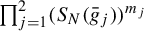 introduces a negligible error.
Since centring preserves the
$L^1$
 -order, we have

We now estimate the error caused by replacing
$g_j$
 with
$h_j$
 . If
$m_j=0$
 , its error term below is omitted. For integers
$r\ge1$
 , using

we obtain

Using (22),

Moreover,

Therefore,

After division by the normalization in (21), this is bounded by
$O(\epsilon _N N^{{m}/{2}}r_N^{a-({md}/{2})}).$
 Since
$Nr_N^d\to \infty $
 , choosing
$\epsilon _N=N^{-B}$
 with
$B>0$
 sufficiently large makes this term
$o(1)$
 . Thus, the error caused by replacing
$g_j$
 by
$h_j$
 in (21) is negligible.
Therefore, the claim (21) will follow once we show

Step 2: cluster decomposition. We expand the product

where

Let
$ C> 0 $
 denote a sufficiently large constant. For each
$\textbf {n}= (n_1,\ldots , n_m)\in \{0,\ldots , N-1\}^m$
 , define clusters as follows. There exists a minimal integer
$1 \leq k=k(\textbf {n}) \leq m^2 + 1$
 such that for all
$i, i'\in \{1,\ldots ,m\},$


For
$l\geq 1$
 , we call
$\{i_1,\ldots ,i_l\}\subset \{1,\ldots ,m\}$
 a cluster of
$\textbf {n}$
 if it is a maximal collection with

In such cases, define
$ l $
 as the cluster length. Then, there exists an integer
${1{\kern-1pt}\leq{\kern-1pt} \eta {\kern-1pt}={\kern-1pt} \eta (\textbf {n}) {\kern-1pt}\leq{\kern-1pt} m}$
 such that
$ \textbf {n}$
 consists of the clusters
$\{i^s_1,\ldots , i^s_{l_s}\}$
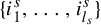 for
$ s = 1,\ldots , \eta $
 , with corresponding lengths
$ l_s $
 .
Equivalently, let
$ k $
 be the smallest integer for which the set
$\{n_i\}$
 can be partitioned into
$\eta $
 clusters of sizes
$l_s$
 , each being a maximal subset where pairwise differences are at most
$C^k \log N$
 and distinct clusters are separated by more than
$C^{k+1} \log N$
 .
For each cluster, let
$b_s=\min_{1\le r\le l_s}n_{i_r^s}$
 . By exponential mixing, we have

Each
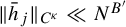
$\bar {h}_j$
 satisfies
$\|\bar {h}_j\|_{C^{\kappa }} \ll N^{B'}$
 for a large constant
$B'>0$
 . Since the time differences within each cluster are at most
$C^k \log N$
 , we obtain

where
$L=\sup _{\|f\|_{C^{\kappa }}=1} \|f\circ T\|_{C^{\kappa }}$
 is the operator norm of
$f\mapsto f\circ T$
 on
$C^{\kappa }$
 .
Consequently, the right-hand side of (25) can be estimated as

which holds for sufficiently large C independent of
$N.$
 After summing over all
$\mathbf n$
 , this error is negligible.
Considering (23) and (26), the claim (21) will follow once we show

Replacing once more the smooth approximations
$\bar {h}_{j(i^s_r)}$
 by
$\bar {g}_{j(i^s_r)}$
 on the left-hand side, similarly to (23), only introduces another negligible error term of order
$o(1)$
 . Therefore, the proof will be finished once we show

Step 3: negligible cluster configurations. Define
$\Delta _\eta = \{\mathbf {n} : \mathbf {n} \text { consists of } \eta \text { clusters}\}.$
 It holds that

Case 3.1:
$\eta>({m}/{2}).$
 At least one cluster is a singleton. Since

then it holds that

Case 3.2:
$\eta <({m}/{2}).$
 If at least one cluster is a singleton, it can be treated as in Case 3.1. If no cluster is a singleton, then all
$l_s \geq 2$
 . Given that

we have

Thus,

Subcase 3.2(i):
$N r_N^d>N^{1/100}$
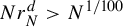 . This bound is of order
$o(N^{{m}/{2}} r_N^{{md}/{2} - m_2 \beta }).$

Subcase 3.2(ii):
$N r_N^d\leq N^{1/100}$
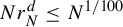
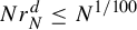 . For each index
$\textbf {n}\in \Delta _{\eta }$
 , we distinguish two cases.
Subcase 3.2(ii-a): all
$n_i$
 within the same cluster are equal for each cluster. Then, there exist
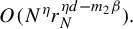
$O(N^\eta )$
 such indices n. Taking into account the estimate in (29), the total contribution from these indices is of order
$O(N^{\eta } r_N^{\eta d - m_2 \beta }).$
Subcase 3.2(ii-b): at least one cluster contains two distinct indices. Then, Lemma 23 provides an additional saving. Using the estimates established in Case 4.1(B) below, (29) can be replaced by

Note that here, the assumption
$N r_N^d\leq N^{{1}/{100}}$
 is used crucially to show
$\log N \asymp |\!\log r_N|$
 .
Since the number of indices
$\mathbf {n}$
 in this subcase is at most
$\#\Delta _{\eta }\ll N^{\eta } (\log N)^m$
 , the total contribution from this case is of order

Combining Subcases 3.2(ii-a) and 3.2(ii-b), it holds that

Using the assumption
$N r_N^d \rightarrow \infty $
 , it follows that
$N^{\eta } r_N^{\eta d - m_2 \beta } =o( N^{{m}/{2}}\, r_N^{{md}/{2} - m_2 \beta })$
 for each
$\eta <({m}/{2})$
 . Therefore, the above bound is of order
$o( N^{{m}/{2}}\,r_N^{{md}/{2} - m_2 \beta })$
 .
In conclusion, all terms in (27) for
$\eta \neq {m}/{2}$
 are asymptotically negligible. Note that, in particular, if m is odd, then (27) is satisfied. So, for the rest of the proof, assume m is even.
Step 4: the critical case
$\eta ={m}/{2}$
 . Unless all the clusters are of length
$2$
 ,
$\textbf {n}$
 must have a singleton. Define

Then, we consider
$\sum _{\mathbf {n}\in \Gamma }\prod _{s=1}^{{m}/{2}}\int (\bar {g}_{j(i^s_1)} \cdot \bar {g}_{j(i^s_2)} \circ T^{|n_{i^s_2}-n_{i^s_1}|})\, {d}\mu .$

Since all terms with singletons are negligible—as in Case 3.1—it is enough to show

Step 4.1: estimates for a single pair. For
$n_i,n_{i'}$
 in the same cluster, we aim to estimate
$\int _M (\bar {g}_{j(i)} \circ T^{n_i})(\bar {g}_{j(i')} \circ T^{n_{i'}})\, {d}\mu $
 . Simplifying notation, we consider

for
$j,j' \in \{1,2\}$
 and
$k=|n_i - n_{i'}| \leq C^{m^2+1} \log N,$
 see (24). In the following, we will distinguish several cases.
We first highlight a technical point. Since
$g_1 = {\mathbf {1}}_{A_N}$
 , the slow recurrence estimate, specifically Lemma 23, is applicable only up to times
$k=C' |\!\log r_N|$
 for a constant
$C'>0$
 , which might be small if
$r_N$
 decays substantially slower than
$1/N$
 .
Case 4.1(A):
$k=0$
 . We consider the cases where
$j=j'=1$
 ,
$j=j'=2$
 and
$j\neq j'$
 . For
$j=j'=1$
 , we use Lemma 22 to obtain

For
$j=j'=2$
 , a straightforward calculation in Euclidean space reveals

where
$\sigma^2 = 1/(2 \alpha - 1)$
 .
A straightforward computation in local coordinates near
$x^*$
 , together with the boundedness of f away from
$x^*$
 , gives

For
$j\neq j'$
 , since the supports of
$g_1$
 and
$g_2$
 are disjoint, we therefore have

Case 4.1(B):
$0<k<C' |\!\log r_N|,$
 where
$C'>0$
 is a sufficiently large constant. For
$j=j'=1$
 , applying Lemma 23 to
$A_N \cap T^{-k}(A_N)$
 with
$A=100m$
 yields

For
$j=j'=2$
 , Lemma 24 with
$A=100m$
 yields

For the cross term
$j\neq j'$
 , we consider the case
$j=1$
 and
$j'=2$
 ; the reverse situation follows analogously.
Let
$\hat {r}_N=r_N|\!\log r_N|^H$
 , where
$H>({100m}/{\beta })$
 is fixed. Since
$A_N$
 is regularly adapted, for sufficiently large N, we have
$A_N\subset B_{\hat {r}_N}(x^*)$
 . Hence,

where

For
$\mathfrak A$
 , note that for sufficiently large N,
$|\!\log r_N|\leq 2|\!\log \hat {r}_N|$
 . Since
$k<C'|\!\log r_N|$
 , we therefore have
$k<2C'|\!\log \hat r_N|.$
 Using slow recurrence with exponent
$A'=Hd+100m$
 and the inclusion
$B_{r_N}(x^*)\subset A_N\subset B_{\hat r_N}(x^*),$
 we obtain

For
$\mathfrak B$
 , using Lemma 22,

Combining the estimates for
$\mathfrak A$
 and
$\mathfrak B$
 gives

Finally, centring does not affect the estimate, so for
$j\neq j'$
 ,

Case 4.1(C):
$k> C' |\!\log r_N|.$
 We emphasize that this case only needs to be considered when
$|\!\log r_N|=o(\log N)$
 . Indeed, all computations here are still inside a cluster, so the relevant time differences satisfy
$k=O(\log N)$
 . If
$|\!\log r_N|$
 is comparable to
$\log N$
 , then taking
$C'$
 large enough makes the condition
$k>C'|\!\log r_N|$
 incompatible with the intra-cluster bound
$k=O(\log N)$
 and this subcase becomes empty. Using (18) with some
$\varepsilon \in (0,r_N)$
 to be determined later, there exists a
$C^{\kappa }$
 smooth function
$\theta :M\rightarrow [0,1]$
 such that

Denote
$\bar {\theta }=\theta - \int _M \theta \, {d}\mu $
 . By applying exponential mixing, we obtain

Choosing
$\varepsilon = e^{-\gamma k/(2 \kappa+1)}$
 guarantees
$\varepsilon <r_N$
 whenever
$C'>(2\kappa +1)/\gamma $
 , since
${k>C'|\!\log r_N|}$
 . We then obtain

If
$k= \lceil C' |\log r_N| \rceil + i$
 for
$i\in \mathbb{N}\cup\{0\},$
 then we have

for large
$C'$
 .
The same argument, with the corresponding smooth approximations of
$g_2$
 and of the cross terms, gives

and

for
$j\neq j'$
 .
Step 4.2: Negligibility outside the diagonal pair configurations. Let

then, using the estimates from
$j\neq j'$
 in Case 4.1(A), and Cases 4.1(B) and 4.1(C) above, we obtain

Note that here we used the fact that all cases, where one of the
$|n_{i^s_1}-n_{i^s_2}|>C'|\!\log r_N|$
 , are negligible by summing the estimate for i from Case 4.1(C).
Step 4.3: The diagonal pair contribution. Using (31) and (32), for
$\mathbf {n}\in \Gamma '$
 , it holds that

If either
$m_1$
 or
$m_2$
 is odd, then
$\Gamma '=\varnothing $
 , since indices of type
$g_1$
 and
$g_2$
 must be paired separately. Otherwise, there are
$(m_1-1)!!$
 and
$(m_2-1)!!$
 possible pairings within each type. For each fixed pairing, this leaves
$m/2$
 free time variables; hence,
$N^{{m}/{2}}$
 choices. The cluster-separation condition excludes only configurations where two such times lie within distance
$O(\log N)$
 , whose number is
$O(N^{({m}/{2})-1}\log N)$
 . Hence,

It follows that

which completes the proof of (30).
3.3 Lightly trimmed SLLN
In this section, we assume that the system
$(M, \mathcal {B}(M), \mu , T)$
 is exponentially mixing and that
$\mathrm {Ord}_{x^*}(f) = d$
 . We establish a lightly trimmed SLLN, which proves Theorem 5. In light of Lemma 19, it suffices to show an SLLN for
$\hat {S}_N^K$
 .
Define

The subsequent lemma bounds the probability that the trimmed sum differs from the original sum by more than a given threshold.
Lemma 27. (Trimmed sum approximation error)
Under the hypothesis above, we have

where the constant
$C_0$
 is defined in (11).
Proof. We observe that

If
$S_N({\mathbf {1}}_{B_{r_N}(x^*)})(x)=m\leq K,$
 then
$\hat {x}_1,\ldots ,\hat {x}_m \in B_{r_N}(x^*)$
 , where
$\hat {x}_j$
 is the jth closest orbit point to
$x^*$
 as defined in §3.1, and consequently,

It follows that

Applying Markov’s inequality, we obtain for sufficiently large
$N,$


We compute the second factorial moment

and consider two cases based on the distance between indices j and
$k.$

Case 1 (long range): if
$k-j> C \log N$
 for some large constant
$C>0$
 , using Lemma 20 and the fact that
$\mu (B_{r_N}(x^*)) \asymp (\log \log N)^6 / (N \log N)$
 , we have

Thus, the contribution from long-range pairs is
$O( (\log \log N)^{12} / (N^2(\log N)^2) ).$
 Since the number of such pairs is at most
$N^2$
 , their total contribution is

Case 2 (short range): by the slow recurrence property with
$A = 3$
 , for large N, we obtain

The number of such pairs is at most
$C N \log N$
 , so their total contribution is

Combining both cases, we have

Finally, we complete the proof using the inequality (35).
Lemma 28. (Ergodic sum of the truncated function)
There exists a sequence
$\epsilon _N \to 0$
 such that

Proof. First, note that

Let
$\varepsilon _N \to 0$
 be chosen such that

Letting
$\epsilon _N=2\varepsilon _N + (\log \log N)^{-1}$
 , Chebyshev’s inequality yields

Applying (20) with
$s=2$
 and
$\beta =d$
 , we obtain

For
$1\le k\le C'|\!\log r_N|$
 , Lemma 24 with
$A=3$
 gives

where
$\bar {f}_N=f_N-\mathbb {E} f_N.$

For
$k=C'|\!\log r_N|+i$
 ,
$i\ge 1$
 , it follows from Case 4.1(C) in the proof of Proposition 25 that for
$C'$
 sufficiently large,

Consequently,

and we conclude

Proof of Theorem 5.

we obtain

Now, consider the subsequence defined by

From the above, we obtain

Therefore, by the first Borel–Cantelli lemma, for
$\mu $
 -almost every
$x,$


For arbitrary
$N \in [N_l, N_{l+1}],$
 the monotonicity of the trimmed sum
$\hat {S}_N^K(f)$
 implies

Taking the limit as
$l \to \infty $
 and observing that
$\lim _{l \to \infty }N_{l+1}/N_l = 1$
 , we conclude that

for
$\mu $
 -almost every x. Finally, Lemma 19 implies that also

Proof of Corollary 7.
Theorem 5 establishes that the normalized trimmed sum
$S_N^K(f)/(N \log N)$
 converges almost surely to
$\operatorname {Res}_{x^*}(f)B_d \rho (x^*) $
 . To pass from trimmed to untrimmed sums, we observe that the contribution from the K largest terms is negligible in probability:

Therefore, the difference between
$S_N(f)/(N \log N)$
 and
$S_N^K(f)/(N \log N)$
 vanishes in probability, and the full sum shares the same limit in probability, that is,

3.4 Intermediately trimmed SLLN
Suppose that the system
$(M, \mathcal {B}(M), \mu , T)$
 is exponentially mixing of all orders, and that
$\mathrm {Ord}_{x^*}(f) = \beta> d$
 . We establish an intermediately trimmed SLLN for ergodic sums, thereby proving Theorem 8. According to Lemma 19, it suffices to prove the SLLN for
$\hat {S}_N^{k(N)}$
 .
The following lemmas are moment estimates that follow directly from Proposition 25.
Lemma 29. Let
$r_N\to 0$
 satisfy
$N r_N^{d} \rightarrow \infty $
 and put

Then, for every fixed
$m\ge 1$
 ,

Proof. For even m, the conclusion follows from Proposition 25 applied with the regularly adapted sequence
$A_N=B_{r_N}(x^*),$
 and the choices
$m_1=0$
 ,
$m_2=m.$
 If m is odd, set
${q=m+1}$
 . Then,

Applying the even case to q gives

which proves the lemma.
Lemma 30. Let
$r_N\to 0$
 with
$N r_N^{d} \rightarrow \infty $
 and put

Then, for every fixed
$m\ge 1$
 ,

Proof. For even m, the result follows by applying Proposition 25 with the regularly adapted sequence
$A_N=B_{r_N}(x^*)$
 and parameters
$m_1=m,m_2=0$
 . The odd case then follows from Hölder’s inequality, exactly as in the proof of Lemma 29.
For the remainder of this section, let
$k(N)\rightarrow \infty $
 be a sequence with
$k(N)=o(N)$
 and define
$r_N>0$
 by

Lemma 31. (Trimmed sum approximation error)
Let
$f_N=f \cdot (1 - {\mathbf {1}}_{B_{r_N}(x^*)} ).$
 Then, for every
$A>0$
 and small
$\epsilon>0,$
 there exists a constant
$C>0$
 such that

Proof. By the continuity of the density function of
$\mu ,$
 we have

Define the event

On
$E_N$
 , the difference between the trimmed sum and the truncated sum satisfies

where
$C_0> 0$
 is the constant from (11) and
$C=C_0(2 B_d\rho (x^*)+10)^{\beta }.$
 It follows that

The probability of the complement
$E_N^c$
 is bounded by

where in the last step, we used the fact that
$N \mu (B_{r_N/2}(x^*))\sim 2^{-d} k(N)$
 .
By Lemma 30, for any integer
$m \geq 2$
 ,

Therefore, applying Markov’s inequality to (37), we deduce

provided that
$m>2A/(1-2\epsilon ).$
 This completes the proof.
Lemma 32. (Ergodic sum of the truncated function)
Under the hypotheses of Lemma 31, for any
$0<\epsilon<1/2$
 and
$A>0,$


Proof. For
$m\geq 2$
 , Lemma 29 yields

where
$\bar {f}_N = f_N - \mathbb {E} f_N$
 . Using Markov’s inequality, it follows that

The desired result follows by selecting an integer
$m>2A/(1-2\epsilon ).$

Proof of Theorem 8.
Using Lemmas 31 and 32, for
$A>0$
 , we have

where the constant
$C>1$
 is the one specified in Lemma 31.
Define the subsequence
$\tilde {N}_l = \lceil 2^{l^{\epsilon }} \rceil $
 and construct
$N_{l,j}$
 recursively by setting
$N_{l,0} = \tilde {N}_l$
 and
$N_{l,j+1} = \min (\tilde {N}_{l+1},N^*),$
 where

This ensures that the sequence
$N_{l,j}$
 increases monotonically from
$\tilde {N}_l$
 to
$\tilde {N}_{l+1},$
 and that the growth of
$k(N)$
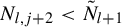
 remains controlled at each step. Specifically, if
$N_{l,j+2}<\tilde {N}_{l+1}$
 , then

Furthermore, since
$k(\tilde {N}_{l+1}) \leq \tilde {N}_{l+1} \leq 2^{(l+1)^{\epsilon }} + 1$
 and the cumulative growth factor over
$2 l^{3\epsilon }$
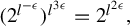
 steps is at least
$(2^{l^{-\epsilon }})^{l^{3\epsilon }} = 2^{l^{2\epsilon }},$
 the sequence must reach
$ \tilde {N}_{l+1}$
 within at most
$2 l^{3\epsilon }$
 steps. Therefore,

Let
$\{N_i\}$
 be the ordered sequence of distinct values from
$N_{l,j}$
 . Then, for sufficiently small
$\epsilon>0$
 and
$A>2 \epsilon ^{-2},$


because
$\lim _{N\rightarrow \infty } {k(N)}/{(\log N)^{\epsilon }} = \infty $
 . By the first Borel–Cantelli lemma and (38), we have

Since

with
$c={1}/({\alpha -1}) \operatorname {Res}_{x^*}(f)B_d^{\alpha } \rho (x^*)^{\alpha }$
 , it follows that

Define two auxiliary trimming sequences as

Since
$\lim _{N\rightarrow \infty } {k_{\pm }(N)}/{k(N)} = 1$
 , Lemmas 31 and 32, as well as (40), also hold for
$k_\pm $
 instead of k; thus, the first Borel–Cantelli lemma implies

For
$N \notin \{N_i\}_{i=1}^\infty $
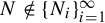 with
$\tilde {N}_l<N_i<N<N_{i+1}<\tilde {N}_{l+1},$
 the construction of
$\{N_i\}$
 and
$k_\pm $
 implies

and

Let x satisfy (42) and (43). By the monotonicity of trimmed sums and applying (44), (45), we obtain

Rewriting this inequality as

and observing that the scaling factors converge to
$1$
 as
$N \to \infty $
 , it follows from the squeeze theorem that

Combining this with (42), this shows that

Finally, Lemma 19 implies that also

3.5 Returns to small balls
The main tool for analysing distributional limits in the lightly trimmed case is the asymptotic Poisson nature of return times to small balls. This section establishes this property.
The Poisson limit theorem for return times has been investigated extensively in the literature. One of the earliest results in a dynamical systems context is due to Pitskel [Reference PitskelPit91], who proved it for mixing Markov chains. Subsequently, the result has been established under various mixing assumptions by many authors; for a comprehensive overview, we refer the reader to the survey [Reference HaydnHay13], especially §5.1 for a discussion of the method of moments. More recently, slow recurrence together with exponential mixing of all orders has been employed in [Reference Dolgopyat, Fayad and LiuDFL22]; see also [Reference AuerAue25].
Specifically, [Reference AuerAue25, Proposition 20] implies that for
$\mu $
 -almost every
$x^* \in M$
 and any finite collection of times
$0<t_1<\cdots <t_J$
 , the finite-dimensional distributions converge weakly as
$r \to 0$
 :

where each
$P(t)$
 is a Poisson random variable with mean t and the vector has independent increments.
Moreover, a minor modification of the argument shows that the convergence in (46) also holds for points
$x^*$
 that are slowly recurrent. If
$\rho (x^*)>0,$
 the measure of
$B_r(x^*)$
 satisfies
$\mu (B_r(x^*))\sim B_d \rho (x^*) r^d$
 , where
$B_d$
 is the volume of the d-dimensional unit ball. Then, (46) becomes

For the arguments that follow, we require a variant of this result in which the number of iterations is fixed while the radius of the balls varies. Although this version can be derived by the same methods, we include a proof for completeness.
Proposition 33. Suppose the system
$(M,\mathcal {B}(M),\mu ,T)$
 is exponentially mixing of all orders. If
$x^* \in M$
 is slowly recurrent and
$\rho (x^*)> 0$
 , then for any
$J\in \mathbb {N}$
 and time points
$0<t_1<t_2<\cdots <t_J$
 , the finite-dimensional distributions converge weakly as
$N \to \infty $
 :

where
$r_N(t)=(t/(B_d\rho(x^*)N))^{1/d}$
 ,
$\chi _{N,t}={\mathbf {1}}_{B_{r_N(t)}(x^*)}$
 and
$(P(t))_{t\geq 0}$
 denotes a standard Poisson process.
Proof. By the method of moments, it suffices to show that for all
$J\geq 1$
 ,
$0=t_0< t_1<\cdots <t_J$
 and
$(m_1,\ldots ,m_J) \in \mathbb {N}^J$
 ,

where
$S_{N,j} =S_N(\chi _{N,t_j})$
 .
For
$N \geq \max _j m_j$
 , we express the product on the left-hand side of (48) as

where, with the convention
$t_0=0$
 and
$\chi _{N,t_0}=0$
 ,

The sum runs over all tuples
$\mathbf {k} = (k_1^1,\ldots , k_{m_1}^1,\ldots , k_1^J,\ldots , k_{m_J}^J)$
 whose entries satisfy
$0 \leq k_1^j < \cdots < k_{m_j}^j \leq N-1$
 for each
$j=1,\ldots ,J$
 . Note that
$\xi _N^{j,i}\cdot \xi _N^{j',i'}=0$
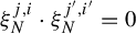 whenever
$j\not =j'$
 and
$k_i^j=k_{i'}^{j'},$
 and therefore, we can restrict the sum to tuples with

For a large constant
$C,$
 let

and

Note that
$ \prod _{j=1}^J \prod _{i=1}^{m_j} \xi _N^{j,i} = 0$
 if
$k^j_i = k^{j'}_{i'}$
 for some
$(j,i)$
 and
$(j',i')$
 with
$j \neq j'$
 . We then decompose the sum in (49) into two components:

where

We aim to prove that

Suppose
$\mathcal {M}=\sum _{j=1}^J m_j.$
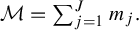 Let us first establish the asymptotic behaviour of
$M_N$
 . For
${\mathbf {k} \in \Delta _N \setminus \Delta _N'}$
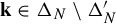 , the indices are well separated. Analogously to Lemma 20, exponential mixing of all orders yields

Summing over
$\mathbf {k}\in \Delta _N\setminus \Delta ^{\prime }_N$
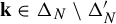 , and noting that

and

we obtain

Now, we turn our attention to
$R_N$
 . Let
$A_N = B_{r_N(t_J)}(x^*)$
 . Note that
$R_N$
 is supported on the set

where
$\varphi _{A_N}(x) = \min \{ k \geq 1 : T^k(x) \in A_N \}$
 is the first return time. By the slow recurrence condition at
$x^*$
 ,

Applying the Cauchy–Schwarz inequality,

Thus, to prove
$\mathbb {E} R_N \rightarrow 0$
 , it suffices to show
$\|R_N\|_{L^2} \ll (\log N)^{\mathcal {M}}$
 . We bound
$\|R_N\|_{L^2}$
 by noting that

where
$S_{N,J} = S_N({\mathbf {1}}_{A_N})$
 and

where
 and
 are the Stirling numbers of the second kind.
Fix
$m \geq 1.$
 We adapt the previous notation for
$t_J,m$
 instead of
$(t_j),(m_j).$
 Then,
$\Delta _N$
 denotes the set of m-tuples
$0 \leq k_1 < \cdots < k_m \leq N-1$
 and
$\Delta _N'$
 is the subset of
$\Delta _N$
 containing tuples where the minimum distance between any two distinct indices is at most
$C \log N.$
 Analogously to (50), we decompose
$\binom {S_{N,J}}{m} = M_{N,m} + R_{N,m}$
 , where
$M_{N,m}$
 and
$R_{N,m}$
 are sums of products of
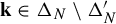
${\mathbf {1}}_{A_N} \circ T^{k_i}$
 over index tuples
$\mathbf {k} \in \Delta _N \setminus \Delta _N'$
 and
$\mathbf {k} \in \Delta _N'$
 , respectively.
As in (52),
$\mathbb {E}M_{N,m}$
 is bounded for each fixed m. It remains to show that

for all
$m = 1, \ldots , 2\mathcal {M}$
 .
We partition
$\Delta _N$
 by defining

Then,
$\Delta _N = \bigcup _{s=1}^m \Delta _N^s$
 , where
$\Delta _N^s = \{ \mathbf {k} : s(\mathbf {k}) = s \}$
 and
$\Delta _N' = \bigcup _{s=1}^{m-1} \Delta _N^s$
 .
For
$s = 1,\ldots , m-1$
 and
$0\leq l_1 < \cdots < l_s \leq N-1$
 with
$\min _r |l_{r+1}-l_r|> C \log N$
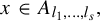
 , define

By exponential mixing of all orders,
$\mu (A_{l_1,\ldots ,l_s})\ll \mu (A_N)^s+o(N^{-s}) \ll N^{-s}$
 . For
${x\in A_{l_1,\ldots ,l_s},}$
 consider

Then,
$|\mathfrak {K}_{l_1,\ldots ,l_s}(x)| \ll (\log N)^m$
 , since the remaining indices must lie within
$C \log N$
 of some
$l_r$
 . Furthermore, for any
$\mathbf {k} \in \mathfrak {K}_{l_1,\ldots ,l_s}(x),$
 the support of the corresponding product satisfies

Thus,

Summing over
$s = 1,\ldots , m-1$
 yields
$\mathbb {E} R_{N,m} \ll (\log N)^m \leq (\log N)^{2\mathcal {M}},$
 thereby completing the proof.
To prepare for a trimmed version, we introduce an alternative representation of the limit in (47) using Poisson point processes.
Definition 34. A random countable set
$\Lambda \subset [0, \infty )$
 is called a (standard) Poisson point process (PPP) if:
-
• for any interval $[t_1,t_2) \subset [0, \infty )$
, the number of points in
$\Lambda \cap [t_1,t_2)$
follows a Poisson distribution with mean
$(t_2-t_1)$
; that is, for
$k\in \mathbb {N},$
$$ \begin{align*} \mathbb{P}(\# (\Lambda \cap [t_1,t_2)) =k) = \frac{(t_2-t_1)^k e^{-(t_2-t_1)}}{k!}; \end{align*} $$
-
• for any collection of disjoint intervals $[s_1, t_1)$
,
$[s_2, t_2)$
,
$\ldots $
,
$[s_n, t_n)\subset [0, \infty )$
, the counts $$ \begin{align*} \#(\Lambda \cap [s_1, t_1)), \#(\Lambda \cap [s_2, t_2)),\ldots, \#(\Lambda \cap [s_n, t_n))\end{align*} $$are independent.





Now, the standard Poisson process
$\mathcal {P}$
 is given by

For
$K\geq 1$
 , the trimmed Poisson point process
$\Lambda ^K$
 is defined as
$\Lambda $
 with the K points closest to the origin removed, that is,

with the convention
$\Lambda ^0=\Lambda $
 .
Remark 35. Given a PPP
$\Lambda $
 , there are i.i.d. standard exponentially distributed random variables
$E_1, E_2, \ldots $
 such that

where
$\xi _k = \sum _{j=1}^k E_j$
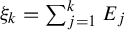 denotes the kth arrival time. Then, the corresponding trimmed PPP is
$\Lambda ^K=\{\xi _k\}_{k\geq K+1}$
 .
Remark 36. The trimmed Poisson point process defined above removes the K points closest to the origin. This differs from the notion of trimmed point processes used elsewhere, for instance, in [Reference Buchmann, Ipsen and MallerBIM17], where trimming refers to discarding the largest jumps of a Lévy process. The two definitions serve different purposes and are not equivalent.
The trimmed version of Proposition 33 is as follows.
Proposition 37. Let
$K\geq 0$
 . Under the same assumptions as in Proposition 33, for any
$0<t_1<\cdots <t_J$
 ,

where
$\Lambda ^K$
 is a trimmed Poisson point process, and
$r_N(t)$
 ,
$\chi _{N,t}$
 are defined as in Proposition 33.
Proof. For
$K=0$
 , the statement reduces to Proposition 33. For
$K\ge 1$
 , the identities

and

show that the conclusion follows immediately from Proposition 33.
3.6 Summation over Poisson point processes
We investigate the asymptotic behaviour of
$\sum _{x\in \Lambda ^K \cap [0,R)} {1}/{x^{\alpha }}$
 for
$\alpha> \tfrac 12$
 , as
$R\rightarrow \infty ,$
 where
$\Lambda ^K$
 denotes a trimmed Poisson point process.
The case
$\alpha> 1$
 can be addressed directly. Using the tail estimate
$\mathbb {P}(\#(\Lambda \cap [n,n+1])> n^{({\alpha -1})/{2}}) \ll e^{-n^{({\alpha -1})/{2}}}$
 for
$n\geq 1$
 and the first Borel–Cantelli lemma, we deduce that almost surely, for all sufficiently large n,
$ \#(\Lambda \cap [n,n+1]) \ll n^{({\alpha -1})/{2}}. $
 It follows that

Moreover, since
$(\Lambda \cap [0,1))$
 is almost surely a finite set and contains no point at
$0$
 ,

Hence,

It remains to study the case
$\alpha \in (\tfrac 12,1]$
 .
Proposition 38. Let
$K \geq 0$
 and
$\alpha>\tfrac 12$
 . Then, there is a non-degenerate random variable Y such that

where

Moreover, the pth absolute moment of Y for any positive integer p satisfies

Proof. For
$\alpha>1$
 , we have already shown in (53) that

Therefore, the desired convergence in distribution holds with
$c_R=0$
 . The finiteness of moments, however, depends on the behaviour near the origin, which will be treated together with the case
$\alpha \in (1/2,1]$
 . Thus, in the main part of the proof, we focus on constructing the centring constants and establishing convergence for
$\alpha \in (1/2,1]$
 .
(i) To establish weak convergence, we first prove convergence for a suitable sequence of centring constants
$c_R>0$
 and a distribution
$\tilde {Y}$
 , without yet claiming non-degeneracy, such that

where
$\Sigma _R=\sum _{x\in \Lambda ^K \cap [1,R)} {1}/{x^{\alpha }}$
 . In Step (iv), we will show that
$c_R$
 may be replaced by the explicit centring constants stated in the proposition.
Once (54) has been established, the conclusion of the proposition follows with

We separate the contribution from
$[0,1)$
 because it is independent of R. Thus, it does not affect the convergence as
$R\to \infty $
 , although it remains part of the limiting random variable and determines the range of p for which
$Y\in L^p$
 .
(ii) For the moment, take
$c_R=\mathbb {E} \Sigma _R$
 . For every even
$k\geq 2$
 , we will show

where
$ \Sigma _{R,R'} =\Sigma _R - \Sigma _{R'}$
 and
$c_{R,R'}=c_R-c_{R'}$
 . This convergence will imply that the sequence
$\{\Sigma _R-c_R\}$
 is Cauchy in
$L^k$
 and, hence, converges in
$L^k$
 to some
$\tilde {Y}$
 . Convergence in
$L^p$
 for every
$p\geq 1$
 then follows immediately from Hölder’s inequality. Once convergence has been established, the limit
$\tilde {Y}$
 does not depend on p and (54) follows.
Let
$\Sigma ^*_{R,R'} = \sum _{x\in \Lambda \cap [R',R)} x^{-\alpha }$
 for
$R>R'>1$
 be the untrimmed sum and
$c^*_{R,R'}=\mathbb {E} \Sigma ^*_{R,R'}$
 . If
$K=0$
 , then
$\Sigma _{R,R'}=\Sigma ^*_{R,R'}.$
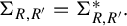 If
$K\ge 1,$
 we observe that

and, consequently,

Therefore, it suffices to prove (55) with
$\Sigma ^*_{R,R'}$
 instead of
$\Sigma _{R,R'}$
 .
Furthermore, it is enough to verify (55) for integer values
$R=n$
 ,
$R'=n'$
 , as the general case follows by standard moment comparison arguments.
(iii) Let
$N= |\Lambda \cap [n',n)|$
 denote the number of points in
$[n',n)$
 , where
$N\sim \text {Poisson}(n-n')$
 . Given
$N=k$
 , the ordered arrival times
$\xi _1, \xi _2,\ldots , \xi _k$
 have the same distribution as k independent random variables uniformly distributed on
$[n',n)$
 , ordered by magnitude. Hence,
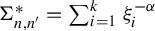
$\Sigma _{n,n'}^*=\sum _{i=1}^k \xi _i^{-\alpha }$
 and

The moment generating function of
$\bar {Y}=\Sigma ^*_{n,n'}-c^*_{n,n'}$
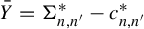 is defined as

We first compute
$\mathbb {E}[e^{t \Sigma ^*_{n,n'}}]$
 using the law of total expectation:

As above, we obtain

Since
$\xi _1\sim \text {Uniform}[n', n)$
 , we have

Thus,

Since
$N\sim \text {Poisson}(n-n')$
 , its probability generating function is
$\mathbb {E}[z^N] = e^{(n-n')(z-1)}$
 . Substituting
$z= M(t)$
 , we obtain

Therefore,

Substituting
$c^*_{n,n'}=\int _{n'}^{n} x^{-\alpha } \, {d} x,$
 we get

It follows that the cumulant generating function is given by

The kth cumulant is
$\kappa _k = K_{\bar {Y}}^{(k)}(0)$
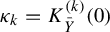 . Noting that
$K_{\bar {Y}}(0) = 0$
 , we further observe that
${\mathbb {E}\bar {Y}= K_{\bar {Y}}'(0) = 0}$
 , which is consistent with the definition of centring. For
$k \geq 2$
 , define
${g(t, u) = e^{t u^{-\alpha }}-t u^{-\alpha }-1}$
 . Then,

Therefore,

This yields

Higher-order moments of
$(\Sigma ^*_{n,n'}-c^*_{n,n'})$
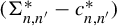 can be expressed in terms of cumulants
$\kappa _n$
 as follows:

where
$B_{k,\ell }(x_1,\ldots , x_{k-\ell +1})$
 denotes the partial Bell polynomial

Given that
$ \kappa _1=0 $
 , all terms with
$ r_1 \geq 1 $
 vanish and the summation is therefore restricted to the case
$ r_1 = 0 $
 . This leads to

If k is even, the dominant term corresponds to the case where
$r_2={k}/{2}$
 and
$ r_j = 0 $
 for all
$ j \neq 2 $
 , which is expressed as

as
$n>n'\to \infty $
 since
$\alpha>\tfrac 12.$

(iv) We now identify the centring constants explicitly. In the case
$\tfrac 12<\alpha \le 1$
 , recall that the centring term used above is
$c_R=\mathbb E\Sigma _R$
 . Since
$\Lambda ^K$
 is obtained from
$\Lambda $
 by removing its first K points
$\xi _1,\ldots ,\xi _K$
 , we have

where, similarly to the above,
$\Sigma _R^*=\sum _{x\in \Lambda \cap [1,R)} x^{-\alpha }$
 denotes the untrimmed sum. Thus,
$c_R$
 is, up to an asymptotically constant additive correction that can be absorbed into the limiting random variable, equal to the expectation of the untrimmed sum
$\Sigma _R^*$
 . Choosing this normalization, we may take

(v) To determine the moments of the limiting random variable, recall from the preceding construction that

Since
$\tilde Y$
 possesses finite moments of all orders, adding
$\tilde Y$
 does not affect the finiteness of the pth moment. Hence, the finiteness or divergence of
$\mathbb {E}(|Y|^p)$
 is determined by the near-origin term

Set
$p_0 = (K+1)/\alpha$
 . It remains to show that this sum lies in
$L^p$
 for
$p<p_0$
 , but not for
$p=p_0$
 .
Condition on
$\xi _{K+1}\in [1/j,1/({j-1}))$
 . By the law of total expectation,

On this event,
$x{\kern-1pt}\ge{\kern-1pt} 1/j$
 for all
$x{\kern-1pt}\in{\kern-1pt} \Lambda ^K\cap [0,1)$
 , so
$\sum x^{-\alpha }{\kern-1pt}\le{\kern-1pt} N j^\alpha $
 with
$N{\kern-1pt}=\#(\Lambda ^K\cap [0,1))$
 . Conditioned on
$\xi _{K+1}$
 , the points in
$(\xi _{K+1},1]$
 form a Poisson process of mean
$1-\xi _{K+1}$
 , so
$N=1+R$
 , where R is Poisson with mean
$1-\xi _{K+1}$
 . Its pth moment is bounded uniformly over
$\xi _{K+1}\in [1/j,1/({j-1}))$
 , yielding

For the probability factor,
$\xi _{K+1}\in [1/j,1/({j-1}))$
 means that there are at least
$K+1$
 points in
$[0,{1}/({j-1}))$
 , but at most K points in
$[0,{1}/{j})$
 . Given
$\#(\Lambda \cap [0,{1}/{j}))=i$
 , one needs at least
$K-i+1$
 points in
$[{1}/{j},{1}/({j-1}))$
 , with corresponding probabilities

Summing over
$i=0,\ldots ,K$
 gives

Combined with (57), the jth term of the sum in (56) is
$O(j^{\alpha p-K-2})$
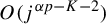 , so the series converges precisely when
$p<p_0$
 .
For the lower bound of the
$p_0$
 th moment: if
$\xi _{K+1}\in [1/j,1/({j-1}))$
 , then we trivially estimate
$\sum x^{-\alpha } \ge \xi _{K+1}^{-\alpha } \gg j^{\alpha }$
 ; hence,

Combining this estimate with (56) and (58) yields

which shows the sum fails to be in
$L^{p_0}$
 .
3.7 Lightly trimmed distributional limits
In this section, we assume that the system
$(M, \mathcal {B}(M), \mu , T)$
 is exponentially mixing of all orders and that
$\mathrm {Ord}_{x^*}(f) = \beta>({d}/{2})$
 . We will show a lightly trimmed distributional law, which establishes Theorem 12. As noted in the previous sections, this is again simpler for
$\hat {S}_N^K$
 , where we simply remove the K closest points to
$x^*$
 . However, unlike our proof for the SLLN, the argument in Lemma 19 is not quite enough to yield a limit theorem for
$S_N^K$
 and a quantitative estimate is required. Recall that by definition,
$\hat {S}_N^K(f)\geq S_N^K(f)$
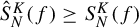 .
Lemma 39. For any fixed integer
$K\geq 0$
 ,

Proof. For
$K=0$
 , we have
$\hat {S}_N^0(f)=S_N^0(f)=S_N(f)$
 and the claim is trivially satisfied. For the rest of the proof, we focus on the case
$K\geq 1$
 .
With the notation from §3.1, each
$y_i$
 satisfies
$d(x^*,y_i)>d(x^*,\hat {x}_K)$
 , since otherwise,
$y_i$
 would be included among the K closest points. Consequently,

Similarly, for each
$\hat {y}_i$
 , we have
$d(x^*, \hat {y}_i) \leq d(x^*, \hat {x}_K)$
 and, thus,

The difference between the trimmed sums is

Substituting the bounds above,

Fix
$\eta> 0$
 and define the set

On
$G_N(\eta )$
 , (59) implies

for
$\eta $
 sufficiently small. It remains to show that
$G_N(\eta )$
 has large probability. By Lemmas 16 and 17, for fixed K,

Since
$\epsilon (r)\to 0$
 as
$r\to 0$
 , we get

For the remaining condition, observe that

Since
$S_N({\mathbf {1}}_{B_{\eta N^{-1/d}}(x^*)})\Rightarrow P(B_d\rho (x^*)\eta ^d)$
 by Proposition 33, where
$P(t)$
 denotes a Poisson random variable with mean t,

Combining the preceding estimates, for every
$\tilde \epsilon>0$
 ,

Letting
$\eta \to 0$
 proves

Before proving Theorem 12, we recall the metric that will be used to study weak convergence. Let
$(\mathcal {M},d_{\mathcal {M}})$
 be a compact metric space and let
$(\tilde {\vartheta }_n)_{n \geq 1}$
 be a sequence of Lipschitz functions on
$\mathcal {M}$
 dense in
$C(\mathcal {M})$
 . Set
$\vartheta _n=\tilde {\vartheta }_n/\|\tilde {\vartheta }_n\|_{\mathrm {Lip}}$
 . For probability measures
$\unicode{x3bb} $
 and
$\unicode{x3bb} '$
 on
$\mathcal {M}$
 , the metric

metrizes weak convergence. In the following proof, we take
$\mathcal {M}=\overline {\mathbb R}=[-\infty ,\infty ]$
 with the metric
$d_{\overline {\mathbb R}}(r,s)=|\text {arctan}\,r - \text {arctan}\,s|,$
 with the usual conventions at
$\pm \infty $
 and write
$D_{\overline {\mathbb R}}$
 for the corresponding metric on probability measures.
Proof of Theorem 12.
(i) We show the claims of the theorem for
$\hat {S}_N^K(f)$
 by proving that

Given Lemma 39, the corresponding result for
$S_N^K(f)$
 follows with the same normalizing constants
$a_N$
 .
(ii) Set
$r_N=(B_d \rho (x^*) N)^{-{1}/{d}}$
 and let
$R>2K$
 , which we regard as fixed for now. For
$N \geq 1$
 , define

and let

Let
$\chi _N = \chi _{N,R} = {\mathbf {1}}_{B_{\rho _N}(x^*)}$
 . Then,

and the proof of Proposition 33, specifically (48), shows that also

It follows that

In the remainder of the proof, we will analyse
$\hat {S}_N^K(f_N)$
 and
$S_N(\bar {f}_N)$
 separately.
Later on, in Step (v), especially (70), we will see that the contribution of
$S_N(\bar {f}_N)/N^\alpha $
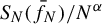 is asymptotically deterministic, in the sense that its fluctuations around its expectation vanish. Therefore, for the main part of the proof, we focus on
$\hat {S}_N^K(f_N)$
 .
(iii) Let
$m\geq 1$
 be a positive integer, which we regard as fixed for now, and partition the ball
$B_{\rho _N}(x^*)$
 into annular regions

and introduce the trimmed counting process

By Proposition 37, the joint convergence

holds. Set
$c=\mathrm {Res}_{x^*}(f) B_d^{\alpha } \rho (x^*)^{\alpha }$
 and define the bounds

and

From the joint convergence (63), we derive

where

Since

for
$x\in A_{N}^{j}$
 and
$1\leq j\leq m-1$
 , where
$\epsilon $
 comes from the local singularity estimate (10), and

we establish the lower bound

and the probabilistic upper bound

(iv) Using Proposition 38, there is a non-degenerate distribution Y and constants
$c_R$
 such that

Moreover, for later use, we explain why the discrete lower and upper sums approximate the Poisson sum. Fix a realization in the full-probability event on which
$\Lambda ^K\cap [0,R)$
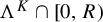 is finite and does not contain
$0$
 . If this set is empty, the desired convergence is immediate. Otherwise, write

For all sufficiently large m, the interval
$[0,R/m)$
 contains no points of
$\Lambda ^K$
 . Hence, for every
$i=1,\ldots ,\ell $
 , there exists a unique
$j_i\in \{1,\ldots ,m-1\}$
 such that

Therefore, for all sufficiently large m,

Since the mesh size
${R}/{m}$
 tends to zero, we have
${Rj_i}/{m},({R(j_i+1)}/{m})\rightarrow x_i$
 for every
$i=1,\ldots ,\ell $
 . Consequently,

Since the exceptional set of realizations has probability zero, we obtain

Consequently, this convergence also holds in distribution.
(v) The conclusion now follows from a diagonal argument. For
$L\ge 1$
 , first choose
${\tilde R_L\ge 8L}$
 sufficiently large such that

where
$D_{\overline {\mathbb R}}$
 is the metric defined in (60). By (67), choose
$\tilde m_L\ge 2L\tilde R_L$
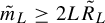 sufficiently large such that

Using (62), (64) and (66), we choose
$\tilde {N}_L$
 sufficiently large so that for all
$N\ge \tilde N_L$
 , we have
$\epsilon (\tilde {R}_L^{{1}/{d}}\, r_{N}) c_{\tilde {R}_L}<({1}/{L}),$
 where
$\epsilon $
 denotes the local singularity estimate (10), and

For
$N\in [\tilde {N}_L, \tilde {N}_{L+1})$
 , set
$R_N=\tilde {R}_L$
 and
$m_N=\tilde {m}_L.$
 By the choice of
$\tilde m_L,\tilde R_L$
 and the first line of (68), the triangle inequality gives

Hence,

Using Lemma 40 with

it follows from (65) and (66) that

It remains to estimate the contribution of
$\bar f_{N,R_N}$
 . Since now we have
$N \rho _N^d\rightarrow \infty $
 , we can apply Proposition 25 with the regularly adapted sequence
$A_N = B_{\rho _N}(x^*)$
 and
${m_1=0,m_2=2}$
 ,

as
$N\rightarrow \infty $
 . By Chebyshev’s inequality, for every
$\delta>0$
 and
$N\in [\tilde N_L,\tilde N_{L+1})$
 ,

Since
$\alpha>\tfrac 12$
 and
$R_N\to \infty $
 , the right-hand side tends to
$0$
 . Therefore,

in probability.
Finally, combining (69), (70) and the second line of (68), we obtain

Consequently,
$N^{-\alpha }(\hat S_N^K(f)-a_N)\Rightarrow cY.$
 Since
$c>0$
 , the random variable
$cY$
 is non-degenerate and relabelling it as Y gives (61).
For
$\tfrac 12<\alpha \leq 1$
 , using the expression for
$c_R$
 obtained in Proposition 38, we have

When
$\alpha>1$
 , we may take
$a_N=0$
 , since
$c_{R_N}=0$
 and
$N^{-\alpha }N\mathbb {E}(\bar f_{N,R_N})\ll R_N^{1-\alpha }\to 0.$

Since the diagonal construction above can be carried out simultaneously for all
${0\le K\le L}$
 at each stage L, the resulting sequence
$R_N$
 , and hence
$a_N$
 , does not depend on K. Its stated asymptotics follow by direct computation.
If
$K=0$
 , then
$\hat S_N^0(f)=S_N^0(f)=S_N(f).$
 If
$K\ge 1$
 , passing from
$\hat {S}_N^K(f)$
 to
$S_N^K(f)$
 follows from Lemma 39.
3.8 Facts about distributional convergence
We collect here two lemmas concerning the metric
$D_{\overline {\mathbb R}}$
 and weak convergence, as defined in §3.7.
Lemma 40. Let
$X_N,Y_N,Z_N,Y$
 be real-valued random variables with

If
$X_N,Y_N,Z_N$
 are defined on a common probability space and

then

Proof. Let
$\xi $
 be a continuity point of the distribution function of
$Y.$
 Then,

and

Lemma 41. Let
$K{\kern-1pt}\geq{\kern-1pt} 1$
 be fixed and suppose that for each N, we have K-dimensional random vectors
$\mathbf {X}_N {\kern-1pt}={\kern-1pt} ( X_N^{(1)},\ldots , X_N^{(K)})$
 ,
$\mathbf {Y}_N {\kern-1pt}={\kern-1pt} ( Y_N^{(1)},\ldots , Y_N^{(K)})$
 and
$\mathbf {Z}_N {\kern-1pt}={\kern-1pt} ( Z_N^{(1)},\ldots , Z_N^{(K)})$
 such that as
$N \to \infty $
 ,

where
$\mathbf {Y} = (Y^{(1)},\ldots ,Y^{(K)})$
 is a K-dimensional random vector. Assume further that for each
$k=1,\ldots ,K$
 and every
$\epsilon \in (0,1)$
 , the following conditions hold as
$N\rightarrow \infty $
 :

Then,

Proof. Choose a sequence
$\epsilon _N \to 0$
 such that all limits in (72) still hold with
$\epsilon $
 replaced by
$\epsilon _N$
 . For each k, define

and

By splitting according to the sign of
$Y_N^{(k)}$
 and using (72), we obtain, for every k,

Since
$\mathbf {X}_N \Rightarrow \mathbf {Y}$
 ,
$\mathbf {Z}_N \Rightarrow \mathbf {Y}$
 and
$\epsilon _N \to 0$
 , Slutsky’s theorem yields

Let

By (73),

For any
$x=(x_1,\ldots ,x_K)\in \mathbb R^K$
 , on the event
$E_N,$
 we have
$\{\widetilde {\mathbf Z}_N\le x\}\subseteq \{\mathbf Y_N\le x\}\subseteq \{\widetilde {\mathbf X}_N\le x\}.$
 Consequently,

Now, let x be a continuity point of the distribution function of
$\mathbf Y$
 . Using (74), both the left and the right sides of the above inequality converge to
$\mathbb P(\mathbf Y\le x).$
 It follows that
$\mathbb P(\mathbf Y_N\le x)\longrightarrow \mathbb P(\mathbf Y\le x)$
 and, therefore,
$\mathbf Y_N\Rightarrow \mathbf Y.$

3.9 Intermediately trimmed distributional limits
In this section, we assume that the system
$(M, \mathcal {B}(M), \mu , T)$
 is exponentially mixing of all orders and that
${\mathrm {Ord}_{x^*}(f) = \beta>({d}/{2})}$
 . We will prove an intermediately trimmed distributional law, which establishes Theorem 15. Without loss of generality, we assume that
$\mathrm {Res}_{x^*}(f) = 1$
 in this section.
Recall that
$x_i$
 is the ith closest point to
$x^*$
 among the
$k(N)$
 points selected to maximize their f values, satisfying

The point
$\hat {x}_i$
 represents the ith closest point to
$x^*$
 among all of
$\{x, T(x), \ldots , T^{N-1}(x)\}$
 . With these definitions, the trimmed sum is given by

and the version defined in §3.1 is given by

To prevent the proof of Theorem 15 from being obscured by technical details, we first explain the idea for the geometrically trimmed sum
$\hat {S}_N^{k(N)}(f)$
 , a simpler case, before proceeding with the full technical arguments.
Let
$r_N>0$
 be chosen by

Since
$\mu (B_r(x^*)) \sim B_d \rho (x^*) r^d$
 , it follows that
$r_N^d\sim {k(N)}/({B_d \rho (x^*) N})$
 . Define
$\hat {f}_N = f\cdot (1-{\mathbf {1}}_{B_{r_N}(x^*)} ).$
 Then,

where

Writing
$\xi _N=d(x^*,\hat {x}_{k(N)})$
 , heuristically, we expect
$\xi _N\approx r_N$
 . We analyse
$\hat W_N$
 by considering the value of
$\xi _N$
 :
-
• if $\xi _N\leq r_N$
, then all of the points
$\hat {x}_i$
lie in
$B_{r_N}(x^*)$
; in this case,
$\hat {W}_N$
is the sum of f over all the points in
$B_{r_N}(x^*)$
that are not one of the
$\hat {x}_i$
; -
• otherwise, if $\xi _N>r_N$
, then every point in
$B_{r_N}(x^*)$
is one of the
$\hat {x}_i$
; in this case,
$-\hat {W}_N$
is the sum of f over the remaining points.


In both cases, all of the points that are being summed over are between
$r_N$
 and
$\xi _N$
 ; keeping in mind that
$\xi _N \approx r_N$
 , it follows that

From Corollary 26 with the regularly adapted sequence
$A_N=B_{r_N}(x^*)$
 , it follows that

as
$N\to \infty ,$
 where
$(\mathcal {N}(0,1), \mathcal {N}(0,\sigma ^2))$
 is a vector of independent normal random variables and
$\sigma ^2={1}/({2\alpha -1}).$
 Combining (75), (76) and (77) completes the proof for
$\hat {S}_N^{k(N)}(f)$
 .
The main technical challenge in going from
$\hat {S}_N^{k(N)}$
 to
$S_N^{k(N)}$
 is that if we simply try to split
$S_N^{k(N)}$
 in the same way, setting

there is no analogue of (76).
Motivated by the proof of Lemma 17, instead of balls, we will use superlevel sets of f. Therefore, let

and let
$\unicode{x3bb} _N>0$
 be the unique value such that

From Lemma 42, it follows that

Now, defining

it does hold that

as will be rigorously justified subsequently, in direct analogy with (76).
The preceding heuristic argument can be made rigorous once the assumptions of Corollary 26 have been verified for the superlevel sets
$\Sigma _{\unicode{x3bb} _N}$
 . We therefore show that the sequence
$\Sigma _{\unicode{x3bb} _N}$
 is regularly adapted in the sense of §3.2.
Lemma 42. Let
$R_N\rightarrow \infty $
 . Then, there are
$\epsilon _N \rightarrow 0$
 such that

Proof. Fix a constant
$C_1>\max \{1,C_0^{1/\beta }\}$
 . The result follows from (10) with

Clearly,
$\epsilon _N\to 0$
 . Indeed, if
$d(x,x^*) < (1-\epsilon _N)R_N^{-1/\beta }$
 , then

so
$x \in \Sigma _{R_N}$
 . Conversely, suppose
$x\in \Sigma _{R_N}$
 . By the global estimate
$f(x)\leq C_0d(x,x^*)^{-\beta }$
 , we have
$d(x,x^*)\leq C_0^{1/\beta }R_N^{-1/\beta }<C_1R_N^{-1/\beta }$
 . Applying (10) with radius
$C_1R_N^{-1/\beta }$
 then yields

and therefore,

Thus,
$x\in B_{(1+\epsilon _N)R_N^{-1/\beta }}(x^*)$
 .
A direct corollary of Lemma 42 is that for
$R_N \to \infty $
 ,

Lemma 43. For
$R_N\rightarrow \infty $
 and
$\epsilon _N \rightarrow 0$
 , there exist
$C^{\kappa }$
 functions
$h_N:M\rightarrow [0,1]$
 such that
${\mathbf {1}}_{\Sigma _{R_N}}\leq h_N\leq {\mathbf {1}}_{\Sigma _{R_N-\epsilon _N}}$
 ,

Proof. Let
$\theta _N:[0,\infty ) \rightarrow [0,1]$
 be a smooth function with:
-
• $\theta _N(r)=1$
if
$r\geq R_N$
; -
• $\theta _N(r)=0$
if
$r\leq R_N-\epsilon _N$
; and -
• $\|\theta _N\|_{C^{\kappa }} \ll \epsilon _N^{-\kappa }$
.



Define
$h_N(x)=\theta _N(f(x))$
 for
$x\neq x^*$
 and
$h_N(x)=1$
 for
$x=x^*.$
 We verify the required properties for
$h_N$
 . Using (80), it follows that
$h_N= 1$
 on
$\Sigma _{R_N} \supset B_{R_N^{-1/\beta }/2}(x^*)$
 and
$h_N= 0$
 outside
$\Sigma _{R_N-\epsilon _N} \subset B_{2R_N^{-1/\beta }}(x^*)$
 . Therefore, the standard
$C^\kappa $
 composition estimate implies that

However, to estimate
$\|{\mathbf {1}}_{\Sigma _{R_N}}-h_N\|_{L^1} \leq \mu (R_N-\epsilon _N \leq f \leq R_N)$
 , write
$f(x) = \phi (x) \cdot g(x)$
 with
$\phi (x) = d(x^*, x)^{-\beta }$
 and
$g\in C^{\kappa }$
 as in Definition 2. Using the product rule
$D_x f=D_x \phi \cdot g(x)+\phi (x) \cdot D_x g$
 and recalling that, by assumption,
$g(x^*)=\mathrm {Res}_{x^*} (f)=~1$
 , we have

For
$t \in [R_N-\epsilon _N, R_N]$
 , the level set
$L_t=\{f=t\}$
 is a
$C^{\kappa }$
 -regular
$(d-1)$
 -dimensional hypersurface and its
$(d-1)$
 -dimensional Hausdorff measure scales as
$H^{d-1}(L_t)=O(t^{-(d-1)/\beta })=O(R_N^{-(d-1)/\beta })$
 . Indeed, even though
$L_t$
 is not simply a hypersphere, its deviation from the hypersphere is determined by g, a
$C^{\kappa }$
 function whose derivative is bounded. By the co-area formula,

On
$L_t$
 , it holds that
$\|D_x f\| \asymp R_N^{1 + 1/\beta }$
 according to (82), so (83) is bounded above by
$O(\epsilon _N R_N^{-1/\alpha -1})$
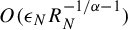 . Hence,

The previous two lemmas show that
$\Sigma _{\unicode{x3bb} _N}$
 is regularly adapted and Corollary 26 can be applied.
Lemma 44. Let
$\unicode{x3bb} _N>0$
 be chosen such that

where
$\Sigma _R=\{f\ge R\},$
 and define

Assume
$k(N)\to \infty $
 and
$k(N)=o(N)$
 . Then,

where
$(\mathcal {N}(0,1), \mathcal {N}(0,\sigma ^2))$
 is a vector of independent normal random variables, and

Proof. By Lemmas 42 and 43, the superlevel sets
$\Sigma _{\unicode{x3bb} _N}$
 form a regularly adapted sequence. Moreover, their effective radii satisfy

In particular,
$Nr_N^d\sim {k(N)}/({B_d\rho (x^*)})\to \infty .$
 Applying Corollary 26 with
$A_N=\Sigma _{\unicode{x3bb} _N}$
 , the claim follows.
Lemma 45. Under the same hypotheses as Lemma 44, for every
$t>0$
 , we have

where
$\mathcal {N}(0,v)$
 is a normal distribution with mean
$0$
 and variance v.
Proof. Fix
$t>0$
 and set
$\tilde {\unicode{x3bb}} _N=t\unicode{x3bb} _N$
 ,
$\tilde k(N)=N\mu (\Sigma _{\tilde {\unicode{x3bb}} _N}).$
 Since
$\mu (\Sigma _R)\sim B_d\rho (x^*)R^{-({1}/{\alpha })}$
 , we have
$\tilde k(N)\sim B_d\rho (x^*)N (t\unicode{x3bb} _N)^{-({1}/{\alpha })}\sim t^{-({1}/{\alpha })}k(N).$
 Applying Lemma 44 with
$\tilde {\unicode{x3bb}} _N$
 and
$\tilde k(N)$
 gives

Now, rewrite

Since
$\tilde k(N)/k(N)\to t^{-1/\alpha }$
 , the desired result follows by Slutsky’s theorem.
Letting

and with
$W_N$
 defined as in (78), we have

The conclusion of the theorem will follow once we show:
-
(A)
$$ \begin{align*} \frac{S_N(f_N)-N \mathbb{E} f_N}{B_d^{\alpha} \rho(x^*)^{\alpha} N^{\alpha} k(N)^{({1}/{2})-\alpha}} \Rightarrow \mathcal{N}(0,\sigma^2) \quad \text{as } N \rightarrow\infty, \end{align*} $$where
$$ \begin{align*} \sigma^2 = \frac{1}{2\alpha - 1}; \end{align*} $$
-
(B)
$$ \begin{align*} \frac{W_N}{B_d^{\alpha} \rho(x^*)^{\alpha} N^{\alpha} k(N)^{({1}/{2})-\alpha}} \Rightarrow \mathcal{N}(0,1) \quad \text{as } N \rightarrow\infty; \end{align*} $$
-
(C) $(S_N(f_N)-N\mathbb {E} f_N) / (B_d^{\alpha } \rho (x^*)^{\alpha } N^{\alpha } k(N)^{\tfrac 12-\alpha })$
is asymptotically independent of
$W_N /(B_d^{\alpha } \rho (x^*)^{\alpha } N^{\alpha } k(N)^{\tfrac 12-\alpha })$
.


Recall that
$W_N = S_N(f \cdot {\mathbf {1}}_{\Sigma _{\unicode{x3bb} _N}}) - \sum _{i=1}^{k(N)} f(x_i),$
 where
$x_1,\ldots ,x_{k(N)}$
 are the orbit points where f assumes the largest values. Now, one of two alternatives can happen:
-
(i) if $f(x_i) \geq \unicode{x3bb} _N$
for all
$1 \leq i \leq k(N)$
, then
$W_N$
is the sum of
$f(y)$
over all points
$y \in \Sigma _{\unicode{x3bb} _N}$
that are not among the
$x_i$
values, and hence,
$W_N \geq 0$
; -
(ii) otherwise, there exists some i with $1 \leq i \leq k(N)$
such that
$f(x_i) < \unicode{x3bb} _N$
; in this case, all points in
$\Sigma _{\unicode{x3bb} _N}$
are already included among the
$x_i$
values and
$-W_N$
equals the sum of f over those
$x_i$
lying outside
$\Sigma _{\unicode{x3bb} _N}$
, so
$W_N< 0$
.


In both situations,
$W_N$
 is (up to sign) a sum of
$f(y)$
 over certain orbit points. We prove upper and lower bounds for
$W_N$
 in both cases.
Notice first a simple lower bound. In Case (i), each term
$f(y)$
 satisfies
$f(y)\geq \unicode{x3bb} _N$
 because
$y\in \Sigma _{\unicode{x3bb} _N}$
 ; in Case (ii), each term satisfies
$f(y)<\unicode{x3bb} _N$
 because
$y\notin \Sigma _{\unicode{x3bb} _N}$
 . The signed number of terms is
$S_N({\mathbf {1}}_{\Sigma _{\unicode{x3bb} _N}})-k(N)$
 , which is negative in Case (ii). Thus, in both cases,

We now turn to obtaining a probabilistic upper bound for
$W_N$
 in Case (i). Let
${J=S_N({\mathbf {1}}_{\Sigma _{\unicode{x3bb} _N}})-k(N)}$
 and denote

Then,
$W_N=\sum _{j=1}^J f(y_j)$
 . If

then
$J\geq 1$
 and at least one of the
$y_j$
 values satisfies
$f(y_j)>(1+\epsilon )\unicode{x3bb} _N$
 . Since the
$x_i$
 values are defined as the points with the largest f-values, it follows that
$f(x_i)\geq f(y_j)>(1+\epsilon )\unicode{x3bb} _N$
 for all
$i=1,\ldots , k(N)$
 . Consequently,

Hence,

For
$t>0$
 , Lemma 45 gives

Applying (87) with
$t=1+\epsilon $
 , we obtain

Moreover, (81) implies that

Thus, for all sufficiently large N,

with some
$c(\epsilon )>0$
 . Using (88) and (89), we have

Combining this with (86) proves

Moreover, using (87) with
$t=1$
 , we have
$\lim _{N\rightarrow \infty } \mu (W_N=0)=0.$
 Therefore,

For Case (ii), we argue similarly: if
$f(x_i) < (1-\epsilon )\unicode{x3bb} _N$
 for some
$1\leq i\leq k(N)$
 , then
$\Sigma _{(1-\epsilon )\unicode{x3bb} _N}$
 contains at most
$k(N)-1$
 of the orbit points, so
$S_N({\mathbf {1}}_{\Sigma _{(1-\epsilon )\unicode{x3bb} _N}}) \le k(N)-1.$
 Then, the same CLT argument using (87) gives

Now, define

and

Equations (85), (91) and (92) show that
$X_N^{(1)}$
 ,
$Y_N^{(1)}$
 ,
$Z_N^{(1)}$
 satisfy the hypotheses of Lemma 41. Thus, once we prove

where the two limiting normal variables are independent and
$\sigma ^2={1}/({2\alpha -1})$
 , Lemma 41 will imply the corresponding convergence

This is exactly the content of parts (A)–(C). Together with Lemma 44, we can conclude the proof.
Proof of Theorem 15.
Lemma 44 shows that

as
$N\to \infty ,$
 where
$(\mathcal {N}(0,1), \mathcal {N}(0,\sigma ^2))$
 is a vector of independent random variables and

By (85), (91) and (92), we can apply Lemma 41 with

where
$W_N$
 is defined in (78), and

and it follows that

This proves parts (A)–(C), and thus finishes the proof of convergence. Finally, the claimed asymptotic expression for
$a_N$
 can be readily derived from the relation
$a_N=N\mathbb {E}f_N$
 .
Acknowledgements
The authors would like to thank Dmitry Dolgopyat for helpful discussions and the University of Maryland, where this project was initiated, for its hospitality.
Funding
During this project, M.A. was partially supported by the Austrian Science Fund (FWF), P 33943-N and by the Australian Research Council (FT240100592). S.L. was partially supported by National Natural Science Foundation of China Nos. 12501237 and 12671228, and Natural Science Foundation of Beijing No. 1244041.

 Open access

