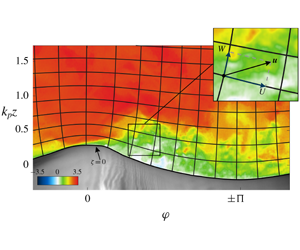
1 Introduction
The investigation of shear flows with streamline curvature are generally challenging problems in fluid mechanics with various applications in engineering and science. Boundary layer flows, in particular, are strongly affected by even a mild surface curvature through the production of additional rates of strain (Bradshaw Reference Bradshaw1973). Although the effects of curvature on turbulent flows over convex and concave solid and fixed surfaces with a mild curvature have been extensively investigated theoretically (e.g. Bradshaw Reference Bradshaw1969; So Reference So1975; Hall & Horseman Reference Hall and Horseman1991; Holloway & Tavoularis Reference Holloway and Tavoularis1998), experimentally (e.g. So & Mellor Reference So and Mellor1973; Ramaprian & Shivaprasad Reference Ramaprian and Shivaprasad1978, Reference Ramaprian and Shivaprasad1982; Hoffmann, Muck & Bradshaw Reference Hoffmann, Muck and Bradshaw1985; Barlow & Johnston Reference Barlow and Johnston1988; Holloway & Tavoularis Reference Holloway and Tavoularis1992; Holloway, Roach & Akbary Reference Holloway, Roach and Akbary2005) and numerically (e.g. Moser & Moin Reference Moser and Moin1987; Neves, Moin & Moser Reference Neves, Moin and Moser1994; Kim & Rhode Reference Kim and Rhode2000; Blin, Hadjadj & Vervisch Reference Blin, Hadjadj and Vervisch2003; Dave, Azih & Yaras Reference Dave, Azih and Yaras2013) over the past decades, there exist substantially fewer studies of the flow in the boundary layer over liquid, propagating surface waves (e.g. Takeuchi, Leavitt & Chao Reference Takeuchi, Leavitt and Chao1977; Hsu, Hsu & Street Reference Hsu, Hsu and Street1981; Hsu & Hsu Reference Hsu and Hsu1983; Sullivan, McWilliams & Moeng Reference Sullivan, McWilliams and Moeng2000; Yang & Shen Reference Yang and Shen2010; Buckley & Veron Reference Buckley and Veron2016). Thus, the current understanding of airflow over surface waves, for example, remains hampered by the complexities associated with the geometrical shape of surface waves. It is observed, in general, that the surface curvature not only changes the mean velocity profiles, but also exerts considerable influences on the fluctuation velocity components, shear stress and turbulent stress compared to similar flows over flat surfaces.
To capture these effects of curvature on the structure of the fluid flow, it is practical to express the governing equations of motion in general orthogonal or non-orthogonal coordinates. Indeed, the additional production, convection and diffusion terms due to the curvature of flow appear explicitly in those kinds of coordinate systems (Bradshaw Reference Bradshaw1973; Moser & Moin Reference Moser and Moin1987). One way to transform the equations of motion from rectangular coordinates to the general coordinates is to transform the coordinate system but not the dependent flow variables such as velocity components. That is, the rectangular flow field is interpreted in a curvilinear coordinate system. For the study of water waves, for example, this approach has been employed by Hsu et al. (Reference Hsu, Hsu and Street1981), Hsu & Hsu (Reference Hsu and Hsu1983), Sullivan et al. (Reference Sullivan, McWilliams and Moeng2000), Shen et al. (Reference Shen, Zhang, Yue and Triantafyllou2003), Yang & Shen (Reference Yang and Shen2010, Reference Yang and Shen2017), Druzhinin, Troitskaya & Zilitinkevich (Reference Druzhinin, Troitskaya and Zilitinkevich2016) and Yang, Deng & Shen (Reference Yang, Deng and Shen2018), among others, and it yields relatively simple equations where the results can be readily interpreted. Moreover, the experimental realizations, particularly single-point measurements, can be performed quite easily (Hsu et al. Reference Hsu, Hsu and Street1981). Another approach is to completely transform the coordinate system along with the dependent flow variables into the curvilinear coordinate system such that the dependent variables, for example, the velocity components, are aligned with the axes of the new coordinate system (e.g. Gent & Taylor Reference Gent and Taylor1976; Al-Zanaidi & Hui Reference Al-Zanaidi and Hui1984; Shyu & Phillips Reference Shyu and Phillips1990; Longuet-Higgins Reference Longuet-Higgins1998). While this kind of transformation simplifies the theoretical analysis as well as numerical modelling, it is generally impractical for conducting experiments (Hsu et al. Reference Hsu, Hsu and Street1981). It should also be pointed out that although the non-orthogonal coordinates are frequently employed in the simulations of airflow over waves (e.g. Sullivan et al. Reference Sullivan, Edson, Hristov and McWilliams2008; Yang & Shen Reference Yang and Shen2010; Hara & Sullivan Reference Hara and Sullivan2015; Xuan, Deng & Shen Reference Xuan, Deng and Shen2019; Hao & Shen Reference Hao and Shen2019) mainly due to convenience in grid generation, they introduce additional complexities in the governing equations. These complexities are primarily associated with the presence of the covariant and contravariant velocity components that leads to different forms of the governing equations. Furthermore, the general curvilinear non-orthogonal coordinates give rise to extra metric tensors, and besides that, the fields in the conservation equations might not have their usual physical meanings (see Richmond, Chen & Patel Reference Richmond, Chen and Patel1986; Finnigan Reference Finnigan2004). However, the governing equations are significantly more straightforward in the orthogonal coordinate systems and preserve much of the analytical simplicity of their counterpart equations in the Cartesian coordinates. The main reason is that no distinction between covariant and contravariant vector and tensor fields exists for the orthogonal coordinate systems.
In the study of ocean surface waves, the wave-coherent motion poses serious challenges to the full transformation of the problem where the separation of mean, wave, and turbulent components is required for a complete treatment of the wave–turbulence interaction (Einaudi & Finnigan Reference Einaudi and Finnigan1993). The triple decomposition of flow field variables into mean, wave and turbulent components was first introduced by Hussain & Reynolds (Reference Hussain and Reynolds1972) and has been extensively applied to air–sea interaction studies. A great number of these numerical and experimental studies, however, are carried in a fixed Cartesian frame of reference (e.g. Finnigan & Einaudi Reference Finnigan and Einaudi1981; Einaudi & Finnigan Reference Einaudi and Finnigan1993; Mastenbroek et al. Reference Mastenbroek, Makin, Garat and Giovanangeli1996; Makin & Kudryavtsev Reference Makin and Kudryavtsev1999; Hara & Belcher Reference Hara and Belcher2004; Rutgersson & Sullivan Reference Rutgersson and Sullivan2005). In such coordinate systems, the wave-associated motions cannot be captured below the highest wave crest (Sullivan et al. Reference Sullivan, McWilliams and Moeng2000; Hara & Sullivan Reference Hara and Sullivan2015), thereby demonstrating the importance of employing a wave-following coordinate system. It should also be noted here that while recent computational studies now routinely employ the algebraic mapping to investigate the wave-induced motions very close to the surface and to address difficulties associated with the non-rectangular physical domain over surface waves, experimental studies have just begun to report such data using wave-following coordinate systems (e.g. Buckley & Veron Reference Buckley and Veron2016, Reference Buckley and Veron2017).
Air–sea interaction studies investigating fluid flow, including continuity, momentum and kinetic energy equations along with the corresponding triple-decomposed equations in a general coordinate system are extremely sparse. Gent & Taylor (Reference Gent and Taylor1976) expressed the conventional Reynolds decomposed continuity, momentum and turbulent energy equations in a wave-following curvilinear coordinate system proposed by Benjamin (Reference Benjamin1959) in order to numerically investigate the two-dimensional (2-D) flow field in a turbulent boundary layer over water waves. The mean governing equations were then closed by the use of an isotropic eddy viscosity model. The equations of 2-D turbulent fluid motion were also derived for an orthogonal streamline coordinate system by Finnigan (Reference Finnigan1983). It was shown that the transformed mean equations for the first and second moments of velocity involve explicit extra terms representing the influences of streamline curvature and the acceleration of the mean flow. These Reynolds decomposed equations were also expressed by Kantha & Rosati (Reference Kantha and Rosati1990) in generalized orthogonal curvilinear coordinates to study the influence of streamline curvature on small-scale turbulence. The algebraic transformation of the governing equations into a surface-fitted curvilinear coordinate system has been widely employed in computational studies of surface waves over the past decades. In order to investigate the turbulent flow over water waves, a 2-D conformal and orthogonal transformation was used by Sullivan et al. (Reference Sullivan, McWilliams and Moeng2000) to map the physical domain on to a computational grid, and, consequently, transform only the coordinates in the governing equations into a surface-fitted, orthogonal coordinate system. To examine the wind–wave interaction in the marine boundary layer, Sullivan et al. (Reference Sullivan, Edson, Hristov and McWilliams2008) expressed the 2-D large-eddy simulation (LES) equations including mass conservation, momentum and energy transport equations in a non-orthogonal, hybrid rectangular–curvilinear computational coordinate system through introducing the contravariant flux velocities (see also Sullivan et al. (Reference Sullivan, McWilliams and Moeng2000) and Sullivan, McWilliams & Patton (Reference Sullivan, McWilliams and Patton2014)). The ensemble-averaged equations for the momentum and energy budgets are further derived by Sullivan et al. (Reference Sullivan, Banner, Morison and Peirson2018) in similar hybrid computational coordinates where the vertical lines are held fixed while the horizontal axis is wave-following.
A comprehensive analysis of the wave boundary layer turbulence over surface waves in a strongly forced condition was carried out recently by Hara & Sullivan (Reference Hara and Sullivan2015). In their study, the dynamical governing equations along with the corresponding mean, wave and turbulent equations were derived in a hybrid, wave-following coordinate system similar to the one used by Sullivan et al. (Reference Sullivan, McWilliams and Patton2014) and Sullivan et al. (Reference Sullivan, Banner, Morison and Peirson2018). The triple decomposition formulations in wave-following coordinates define the expression for the wave-induced stress as a sum of the wave and pressure stresses compared to the traditional definition (e.g. Makin & Kudryavtsev Reference Makin and Kudryavtsev1999; Hara & Belcher Reference Hara and Belcher2004) in terms of the wave-coherent velocity components. Finally, there are some recent attempts to express the viscous tangential stresses at the air–water interface in an orthogonal wave-following coordinate system (see Buckley & Veron Reference Buckley and Veron2017; Iafrati, De Vita & Verzicco Reference Iafrati, De Vita and Verzicco2019), but we note that these estimates are valid only in the linear wave limit.
In the study of turbulent flows over propagating surface waves, the necessity of employing a wave-following coordinate system has been recognized (e.g. Hsu et al. Reference Hsu, Hsu and Street1981; Sullivan et al. Reference Sullivan, McWilliams and Moeng2000; Hara & Sullivan Reference Hara and Sullivan2015), and, therefore, as mentioned above, the algebraic mapping of rectangular coordinates into wave-following coordinates has commonly been employed in theoretical and numerical studies, and just recently, in laboratory measurements. However, the further step of fully transforming the governing equations with the dependent flow variables into those coordinate systems is rarely taken, and to the best of the authors’ knowledge, the decomposed mean, wave and turbulent equations required for the complete treatment of wave–turbulence interaction are not yet fully derived. This is in part due to the mathematical difficulties associated with the curvilinear coordinates and the fact that experimental studies have not been able to estimate the additional geometric terms appearing in the transformed equations. Therefore, in the current study we present the fully transformed governing equations of fluid flow including continuity, momentum and kinetic energy equations in the wave-following orthogonal curvilinear coordinate system along with the triple-decomposed form of those equations. The orthogonal general coordinate system is physically intuitive and appropriate for the study of the turbulent flow over surface waves since it can provide an alternative framework in which the surface-parallel continuity, momentum and energy budget equations can be thoroughly investigated, which leads to a better physical interpretation of many quantities in the governing equations. The complete transformation of the governing equations also directly allows us to account for the streamline curvature. Finally, we simplify the equations for the mean, wave and turbulent fields using classical boundary layer approximations. The fluid flow governing equations in orthogonal curvilinear coordinates are presented in § 2, and the corresponding triple-decomposed equations are expressed in § 3. We narrow our focus to the weakly nonlinear waves in § 4 and perform a boundary layer scaling. The triple-decomposed equations for the boundary layer are then derived in § 4.1. We finally offer a brief conclusion in § 5. In appendix A, we provide the velocity–vorticity formulations in orthogonal curvilinear coordinates. Analyses of experimental data using the framework developed in this paper are presented in a companion paper (Yousefi, Veron & Buckley Reference Yousefi, Veron and Buckley2020).
2 Fluid flow governing equations
The governing equations of fluid motion, including continuity, momentum and kinetic energy equations in a turbulent flow are first derived in an orthogonal curvilinear coordinate system. These equations are then decomposed into mean, wave-induced and turbulence components by employing the triple decomposition technique. To express the equations of motion, the flow is assumed to have a constant density, a constant kinematic viscosity and velocity components  $\boldsymbol{u}=(u_{1},u_{2},u_{3})$ in
 $x_{1}$,
 $x_{2}$ and
 $x_{3}$ directions, respectively. The continuity, momentum and energy equations for an incompressible fluid can be written in an invariant vector form as
 $$\begin{eqnarray}\displaystyle & \displaystyle \unicode[STIX]{x1D735}\boldsymbol{\cdot }\boldsymbol{u}=0, & \displaystyle\end{eqnarray}$$
 $$\begin{eqnarray}\displaystyle & \displaystyle \unicode[STIX]{x1D70C}\frac{\unicode[STIX]{x2202}\boldsymbol{u}}{\unicode[STIX]{x2202}t}+\unicode[STIX]{x1D70C}(\boldsymbol{u}\boldsymbol{\cdot }\unicode[STIX]{x1D735})\boldsymbol{u}=-\unicode[STIX]{x1D735}p+\unicode[STIX]{x1D735}\boldsymbol{\cdot }\unicode[STIX]{x1D749}, & \displaystyle\end{eqnarray}$$
 $$\begin{eqnarray}\displaystyle & \displaystyle \unicode[STIX]{x1D70C}\frac{\unicode[STIX]{x2202}e}{\unicode[STIX]{x2202}t}+\unicode[STIX]{x1D70C}(\unicode[STIX]{x1D735}\boldsymbol{\cdot }e\boldsymbol{u})=-\unicode[STIX]{x1D735}\boldsymbol{\cdot }(p\boldsymbol{u})+(\unicode[STIX]{x1D735}\boldsymbol{\cdot }\unicode[STIX]{x1D749})\boldsymbol{\cdot }\boldsymbol{u}, & \displaystyle\end{eqnarray}$$
where  $\boldsymbol{u}$ is the velocity vector,
 $\unicode[STIX]{x1D70C}$ is the density and
 $p$ is the pressure which includes the static gravity term
 $gz$. Also
 $\unicode[STIX]{x1D749}=2\unicode[STIX]{x1D707}\unicode[STIX]{x1D64E}$ is the viscous stress tensor,
 $\unicode[STIX]{x1D707}$ is the dynamic viscosity,
 $2\unicode[STIX]{x1D64E}=(\unicode[STIX]{x1D735}\boldsymbol{u}+(\unicode[STIX]{x1D735}\boldsymbol{u})^{\text{T}})$ is the strain rate tensor and
 $e=(\boldsymbol{u}\boldsymbol{\cdot }\boldsymbol{u})/2$ is the kinetic energy. The velocity gradient tensor is noted as
 $\unicode[STIX]{x1D735}\boldsymbol{u}$ and
 $(\unicode[STIX]{x1D735}\boldsymbol{u})^{\text{T}}$ denotes its transpose.
2.1 Orthogonal curvilinear coordinates
Fixed rectangular coordinate systems are not able to capture the effects of streamline curvature and, particularly in the study of wind waves, no spatially or temporally averaged information can be obtained beneath the highest wave crest (e.g. Sullivan et al. Reference Sullivan, McWilliams and Moeng2000; Hara & Sullivan Reference Hara and Sullivan2015). In order to investigate the wave-induced motions near the interface and/or below the wave crest, it is thus necessary to employ a coordinate system that closely follows the wave shapes. For example, Hara & Sullivan (Reference Hara and Sullivan2015) and Yang & Shen (Reference Yang and Shen2017) recently employed a coordinate system that follows the vertical displacement due to the surface waves. However, we find that the strictly orthogonal curvilinear coordinate system is practical and physically intuitive. In this section, we derive the continuity, momentum and energy equations in an orthogonal curvilinear coordinate system.
Let  $x_{i}=(x_{1},x_{2},x_{3})$ represent the Cartesian coordinate system and
 $\unicode[STIX]{x1D709}_{i}=(\unicode[STIX]{x1D709}_{1},\unicode[STIX]{x1D709}_{2},\unicode[STIX]{x1D709}_{3})$ represent a set of arbitrary orthogonal curvilinear coordinates. It is well understood that the distinction between covariant and contravariant components in general non-orthogonal curvilinear coordinates vanishes in orthogonal curvilinear coordinate systems. The orthogonal coordinate basis can then be defined as follows (Vinokur Reference Vinokur1974; Redzic Reference Redzic2001; Shikhmurzaev & Sisoev Reference Shikhmurzaev and Sisoev2017):
 $$\begin{eqnarray}\unicode[STIX]{x1D743}_{i}=\frac{\unicode[STIX]{x2202}x_{k}}{\unicode[STIX]{x2202}\unicode[STIX]{x1D709}_{i}}\widehat{\boldsymbol{e}}_{k},\end{eqnarray}$$
where  $\widehat{\boldsymbol{e}}_{k}$ are the corresponding Cartesian orthonormal basis. The base vectors in orthogonal curvilinear coordinates are not necessarily unit vectors. The orthonormal base vectors in orthogonal curvilinear coordinates can be obtained by
 $$\begin{eqnarray}\widehat{\unicode[STIX]{x1D743}}_{i}=\frac{\unicode[STIX]{x1D743}_{i}}{h_{i}},\end{eqnarray}$$
where the quantities  $h_{i}$ are the so-called scale factors of the orthogonal curvilinear coordinate system given by
 $$\begin{eqnarray}\left.\begin{array}{@{}l@{}}(h_{1})^{2}=\left({\displaystyle \frac{\unicode[STIX]{x2202}x_{1}}{\unicode[STIX]{x2202}\unicode[STIX]{x1D709}_{1}}}\right)^{2}+\left({\displaystyle \frac{\unicode[STIX]{x2202}x_{2}}{\unicode[STIX]{x2202}\unicode[STIX]{x1D709}_{1}}}\right)^{2}+\left({\displaystyle \frac{\unicode[STIX]{x2202}x_{3}}{\unicode[STIX]{x2202}\unicode[STIX]{x1D709}_{1}}}\right)^{2},\\[8.0pt] (h_{2})^{2}=\left({\displaystyle \frac{\unicode[STIX]{x2202}x_{1}}{\unicode[STIX]{x2202}\unicode[STIX]{x1D709}_{2}}}\right)^{2}+\left({\displaystyle \frac{\unicode[STIX]{x2202}x_{2}}{\unicode[STIX]{x2202}\unicode[STIX]{x1D709}_{2}}}\right)^{2}+\left({\displaystyle \frac{\unicode[STIX]{x2202}x_{3}}{\unicode[STIX]{x2202}\unicode[STIX]{x1D709}_{2}}}\right)^{2},\\[8.0pt] (h_{3})^{2}=\left({\displaystyle \frac{\unicode[STIX]{x2202}x_{1}}{\unicode[STIX]{x2202}\unicode[STIX]{x1D709}_{3}}}\right)^{2}+\left({\displaystyle \frac{\unicode[STIX]{x2202}x_{2}}{\unicode[STIX]{x2202}\unicode[STIX]{x1D709}_{3}}}\right)^{2}+\left({\displaystyle \frac{\unicode[STIX]{x2202}x_{3}}{\unicode[STIX]{x2202}\unicode[STIX]{x1D709}_{3}}}\right)^{2}.\end{array}\right\}\end{eqnarray}$$
In order to express (2.1) to (2.3) in orthogonal curvilinear coordinates, we will first spell out the differential vector operators including gradient, divergence, curl and Laplacian in orthogonal coordinates. These operators are fairly standard and can be found in the literature (e.g. Aris Reference Aris1962; Batchelor Reference Batchelor1967; Anderson, Tannehill & Pletcher Reference Anderson, Tannehill and Pletcher1984; Redzic Reference Redzic2001; Nikitin Reference Nikitin2006), but we choose to include them here for completeness. Furthermore, in order to substantially simplify the notation in the remainder of this paper, we propose a notation that builds on and modifies the standard Einstein summation convention. Indeed, throughout this work the index notation is such that no summing is carried whenever the indices are enclosed within parentheses. Accordingly, the indices within parentheses only take the value of dummy or free indexes. All other aspects of the summation convention remain unchanged; any index that is repeated twice in any term of expression is called a dummy or repeated index to be summed over the range of its values and any index not repeated is called a free index taking any value in its range. For instance, the suffix  $(i)$ in the following expression only takes the value of the free index
 $i$, i.e.
 $u_{i}u_{j}\unicode[STIX]{x1D705}_{(i)j}=u_{1}u_{1}\unicode[STIX]{x1D705}_{11}+u_{1}u_{2}\unicode[STIX]{x1D705}_{12}+u_{1}u_{3}\unicode[STIX]{x1D705}_{13}$, and the suffix
 $(j)$ in the following expression takes the value of the dummy index
 $j$, i.e.
 $u_{j}u_{j}\unicode[STIX]{x1D705}_{(j)i}=u_{1}u_{1}\unicode[STIX]{x1D705}_{1i}+u_{2}u_{2}\unicode[STIX]{x1D705}_{2i}+u_{3}u_{3}\unicode[STIX]{x1D705}_{3i}$. With this notation, the standard vector and tensor operators can then be expressed in the orthogonal curvilinear coordinate systems in a way that we find elegant and conveniently compact. If
 $\unicode[STIX]{x1D711}$ is an arbitrary scalar,
 $\boldsymbol{A}$ is an arbitrary vector and
 $\unicode[STIX]{x1D64F}$ is an arbitrary tensor field, the expressions for the gradient, divergence, curl and Laplacian operators in the orthogonal curvilinear coordinates become
 $$\begin{eqnarray}\displaystyle & \displaystyle \unicode[STIX]{x1D735}\unicode[STIX]{x1D711}=\frac{1}{h_{(i)}}\frac{\unicode[STIX]{x2202}\unicode[STIX]{x1D711}}{\unicode[STIX]{x2202}\unicode[STIX]{x1D709}_{i}}\widehat{\unicode[STIX]{x1D743}}_{i}, & \displaystyle\end{eqnarray}$$
 $$\begin{eqnarray}\displaystyle & \displaystyle \unicode[STIX]{x1D735}\boldsymbol{\cdot }\boldsymbol{A}=\frac{1}{h}\frac{\unicode[STIX]{x2202}}{\unicode[STIX]{x2202}\unicode[STIX]{x1D709}_{i}}\left(\frac{h}{h_{(i)}}a_{i}\right), & \displaystyle\end{eqnarray}$$
 $$\begin{eqnarray}\displaystyle & \displaystyle \unicode[STIX]{x1D735}\times \boldsymbol{A}=\unicode[STIX]{x1D700}_{ijk}\frac{h_{(i)}}{h}\frac{\unicode[STIX]{x2202}}{\unicode[STIX]{x2202}\unicode[STIX]{x1D709}_{j}}(h_{(k)}a_{k})\widehat{\unicode[STIX]{x1D743}}_{i}, & \displaystyle\end{eqnarray}$$
 $$\begin{eqnarray}\displaystyle & \displaystyle \unicode[STIX]{x1D6FB}^{2}\unicode[STIX]{x1D711}=\frac{1}{h}\frac{\unicode[STIX]{x2202}}{\unicode[STIX]{x2202}\unicode[STIX]{x1D709}_{i}}\left(\frac{h}{h_{(i)}h_{(i)}}\frac{\unicode[STIX]{x2202}\unicode[STIX]{x1D711}}{\unicode[STIX]{x2202}\unicode[STIX]{x1D709}_{i}}\right), & \displaystyle\end{eqnarray}$$
where  $h=h_{1}h_{2}h_{3}$. Furthermore,
 $$\begin{eqnarray}\displaystyle & \displaystyle (\boldsymbol{A}\boldsymbol{\cdot }\unicode[STIX]{x1D735})\boldsymbol{B}=\left[\frac{a_{j}}{h_{(j)}}\frac{\unicode[STIX]{x2202}b_{i}}{\unicode[STIX]{x2202}\unicode[STIX]{x1D709}_{j}}+(a_{i}b_{j}\unicode[STIX]{x1D705}_{(i)j}-a_{j}b_{j}\unicode[STIX]{x1D705}_{(j)i})\right]\widehat{\unicode[STIX]{x1D743}}_{i}, & \displaystyle\end{eqnarray}$$
 $$\begin{eqnarray}\displaystyle & \displaystyle \unicode[STIX]{x1D735}\boldsymbol{\cdot }\unicode[STIX]{x1D64F}=\left[\frac{1}{h}\frac{\unicode[STIX]{x2202}}{\unicode[STIX]{x2202}\unicode[STIX]{x1D709}_{j}}\left(\frac{h}{h_{(j)}}\unicode[STIX]{x1D61B}_{ij}\right)+(\unicode[STIX]{x1D61B}_{ij}\unicode[STIX]{x1D705}_{(i)j}-\unicode[STIX]{x1D61B}_{jj}\unicode[STIX]{x1D705}_{(j)i})\right]\widehat{\unicode[STIX]{x1D743}}_{i}. & \displaystyle\end{eqnarray}$$
In the above equations,  $a_{i}$,
 $b_{i}$ and
 $\unicode[STIX]{x1D61B}_{ij}$ are respectively the components of the vector
 $\boldsymbol{A}$, vector
 $\boldsymbol{B}$ and tensor
 $\unicode[STIX]{x1D64F}$ defined based on the orthonormal basis, and
 $\unicode[STIX]{x1D705}_{ij}$ are the components of the curvature matrix which account for the curvature of the coordinate system and can be defined as
 $$\begin{eqnarray}\boldsymbol{{\mathcal{K}}}=\left[\begin{array}{@{}ccc@{}}{\displaystyle \frac{1}{h_{1}h_{1}}}{\displaystyle \frac{\unicode[STIX]{x2202}h_{1}}{\unicode[STIX]{x2202}\unicode[STIX]{x1D709}_{1}}} & {\displaystyle \frac{1}{h_{1}h_{2}}}{\displaystyle \frac{\unicode[STIX]{x2202}h_{1}}{\unicode[STIX]{x2202}\unicode[STIX]{x1D709}_{2}}} & {\displaystyle \frac{1}{h_{1}h_{3}}}{\displaystyle \frac{\unicode[STIX]{x2202}h_{1}}{\unicode[STIX]{x2202}\unicode[STIX]{x1D709}_{3}}}\\[12.0pt] {\displaystyle \frac{1}{h_{1}h_{2}}}{\displaystyle \frac{\unicode[STIX]{x2202}h_{2}}{\unicode[STIX]{x2202}\unicode[STIX]{x1D709}_{1}}} & {\displaystyle \frac{1}{h_{2}h_{2}}}{\displaystyle \frac{\unicode[STIX]{x2202}h_{2}}{\unicode[STIX]{x2202}\unicode[STIX]{x1D709}_{2}}} & {\displaystyle \frac{1}{h_{2}h_{3}}}{\displaystyle \frac{\unicode[STIX]{x2202}h_{2}}{\unicode[STIX]{x2202}\unicode[STIX]{x1D709}_{3}}}\\[12.0pt] {\displaystyle \frac{1}{h_{3}h_{1}}}{\displaystyle \frac{\unicode[STIX]{x2202}h_{3}}{\unicode[STIX]{x2202}\unicode[STIX]{x1D709}_{1}}} & {\displaystyle \frac{1}{h_{2}h_{3}}}{\displaystyle \frac{\unicode[STIX]{x2202}h_{3}}{\unicode[STIX]{x2202}\unicode[STIX]{x1D709}_{2}}} & {\displaystyle \frac{1}{h_{3}h_{3}}}{\displaystyle \frac{\unicode[STIX]{x2202}h_{3}}{\unicode[STIX]{x2202}\unicode[STIX]{x1D709}_{3}}}\end{array}\right].\end{eqnarray}$$
Thus, all terms in the continuity, momentum and energy equations, (2.1)–(2.3), can now be expressed in orthogonal curvilinear coordinates. The vector operators presented in (2.7)–(2.12) are consistent with those given in the literature, see e.g. Aris (Reference Aris1962), Vinokur (Reference Vinokur1974), Anderson et al. (Reference Anderson, Tannehill and Pletcher1984), Redzic (Reference Redzic2001) and Nikitin (Reference Nikitin2006), but expressed in a compact and practical form.
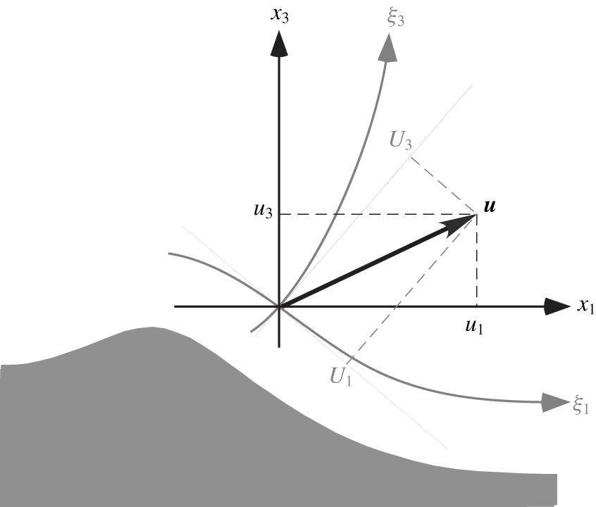
Two-dimensional schematics of the velocity components in Cartesian and orthogonal curvilinear coordinate systems. Here,  $(u_{1},u_{3})=(u,w)$ are components of the velocity vector
 $\boldsymbol{u}$ corresponding to the
 $(x_{1},x_{3})=(x,z)$ Cartesian coordinates and
 $(U_{1},U_{3})=(U,W)$ are the components of the velocity vector
 $\boldsymbol{u}$ corresponding to the arbitrary
 $(\unicode[STIX]{x1D709}_{1},\unicode[STIX]{x1D709}_{3})=(\unicode[STIX]{x1D709},\unicode[STIX]{x1D701})$ orthogonal curvilinear coordinates.

2.2 Continuity, momentum and energy equations
In order to express the fluid governing equations, consider a set of arbitrary orthogonal curvilinear coordinates  $\unicode[STIX]{x1D709}_{i}=(\unicode[STIX]{x1D709}_{1},\unicode[STIX]{x1D709}_{2},\unicode[STIX]{x1D709}_{3})$ with corresponding velocity components
 $\boldsymbol{U}=(U_{1},U_{2},U_{3})$. The velocity components in orthogonal curvilinear coordinates are projections of the velocity vector into the coordinate axes and thus related to the Cartesian velocities by the coordinate transformation. The components of the velocity vector
 $\boldsymbol{u}$ in both Cartesian and orthogonal curvilinear coordinate systems are schematically illustrated in figure 1. Using the vector operators introduced in (2.7)–(2.12), the continuity, momentum and energy equations can be then written as
 $$\begin{eqnarray}\frac{1}{h}\frac{\unicode[STIX]{x2202}}{\unicode[STIX]{x2202}\unicode[STIX]{x1D709}_{i}}\left(\frac{h}{h_{(i)}}U_{i}\right)=0,\end{eqnarray}$$
 $$\begin{eqnarray}\displaystyle & & \displaystyle \displaystyle \frac{\unicode[STIX]{x2202}U_{i}}{\unicode[STIX]{x2202}t}+\frac{U_{j}}{h_{(j)}}\frac{\unicode[STIX]{x2202}U_{i}}{\unicode[STIX]{x2202}\unicode[STIX]{x1D709}_{j}}+(U_{i}U_{j}\unicode[STIX]{x1D705}_{(i)j}-U_{j}U_{j}\unicode[STIX]{x1D705}_{(j)i})\nonumber\\ \displaystyle & & \displaystyle \displaystyle \quad =-\frac{1}{\unicode[STIX]{x1D70C}}\frac{1}{h_{(i)}}\frac{\unicode[STIX]{x2202}p}{\unicode[STIX]{x2202}\unicode[STIX]{x1D709}_{i}}+\frac{1}{\unicode[STIX]{x1D70C}}\left[\frac{1}{h}\frac{\unicode[STIX]{x2202}}{\unicode[STIX]{x2202}\unicode[STIX]{x1D709}_{j}}\left(\frac{h}{h_{(j)}}\unicode[STIX]{x1D70F}_{ij}\right)+(\unicode[STIX]{x1D70F}_{ij}\unicode[STIX]{x1D705}_{(i)j}-\unicode[STIX]{x1D70F}_{jj}\unicode[STIX]{x1D705}_{(j)i})\right],\end{eqnarray}$$
 $$\begin{eqnarray}\frac{\unicode[STIX]{x2202}e}{\unicode[STIX]{x2202}t}+\frac{U_{i}}{h_{(i)}}\frac{\unicode[STIX]{x2202}e}{\unicode[STIX]{x2202}\unicode[STIX]{x1D709}_{i}}=-\frac{1}{\unicode[STIX]{x1D70C}}\frac{U_{i}}{h_{(i)}}\frac{\unicode[STIX]{x2202}p}{\unicode[STIX]{x2202}\unicode[STIX]{x1D709}_{i}}+\frac{1}{\unicode[STIX]{x1D70C}}\left[\frac{U_{i}}{h}\frac{\unicode[STIX]{x2202}}{\unicode[STIX]{x2202}\unicode[STIX]{x1D709}_{j}}\left(\frac{h}{h_{(j)}}\unicode[STIX]{x1D70F}_{ij}\right)+U_{i}(\unicode[STIX]{x1D70F}_{ij}\unicode[STIX]{x1D705}_{(i)j}-\unicode[STIX]{x1D70F}_{jj}\unicode[STIX]{x1D705}_{(j)i})\right],\end{eqnarray}$$
where  $e=(U_{i}U_{i})/2$.
Here, it is noted that the governing equations (2.14)–(2.16) are obtained using a time-independent transformation. The continuity, momentum and energy equations given here for the orthogonal coordinates are quite similar to the conventional Cartesian coordinate system, except for the additional curvature terms that, in fact, account for the curvature of the coordinate system and produced due to the spatial dependence of the base vectors. The Cartesian coordinate equations are simply recovered by noting that  $h_{i}=1$ for rectangular coordinates. The reader may directly verify that the expanded form of the governing equations (2.14)–(2.16) are identical to the continuity and momentum equations given in the literature for an orthogonal curvilinear coordinate system (e.g. Brown & Hung Reference Brown and Hung1977; Hung & Brown Reference Hung and Brown1977; Raithby, Galpin & Van Doormaal Reference Raithby, Galpin and Van Doormaal1986; Blumberg & Herring Reference Blumberg and Herring1987; Nikitin Reference Nikitin2006; Shen et al. Reference Shen, Lu, Wu and Xue2015).
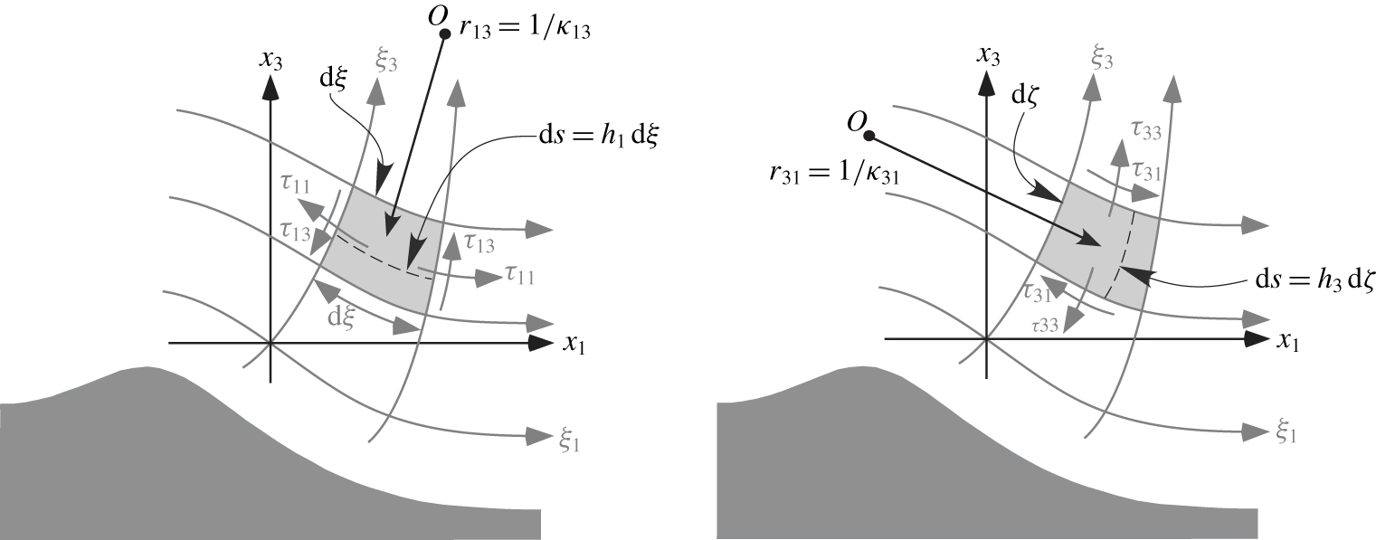
Illustration of the viscous stress field along with the curvature parameter in the  $\unicode[STIX]{x1D709}_{1}{-}\unicode[STIX]{x1D709}_{3}$ plane of an arbitrary orthogonal curvilinear coordinate system. Here,
 $r_{31}=1/\unicode[STIX]{x1D705}_{31}$ and
 $r_{13}=1/\unicode[STIX]{x1D705}_{13}$ are the radius of curvature along the constant
 $\unicode[STIX]{x1D709}_{1}$- and
 $\unicode[STIX]{x1D709}_{3}$-coordinate, respectively, with respect to the
 $\unicode[STIX]{x1D709}_{1}{-}\unicode[STIX]{x1D709}_{3}$ plane. The point where two tangent vectors
 $\unicode[STIX]{x1D709}_{1}$ and
 $\unicode[STIX]{x1D709}_{1}+\text{d}\unicode[STIX]{x1D709}_{1}$ intersect is called the centre of curvature and denoted by the point
 $O$.

Again, the viscous stress is
 $$\begin{eqnarray}\unicode[STIX]{x1D70F}_{ij}=2\unicode[STIX]{x1D707}\unicode[STIX]{x1D61A}_{ij},\end{eqnarray}$$
where the components of the strain rate tensor can now be expressed in an orthogonal coordinate system as
 $$\begin{eqnarray}\unicode[STIX]{x1D61A}_{ij}=\frac{1}{2}\left[\frac{1}{h_{(j)}}\frac{\unicode[STIX]{x2202}U_{i}}{\unicode[STIX]{x2202}\unicode[STIX]{x1D709}_{j}}+\frac{1}{h_{(i)}}\frac{\unicode[STIX]{x2202}U_{j}}{\unicode[STIX]{x2202}\unicode[STIX]{x1D709}_{i}}-(U_{(i)}\unicode[STIX]{x1D705}_{ij}+U_{(j)}\unicode[STIX]{x1D705}_{ji})+2U_{m}\unicode[STIX]{x1D705}_{(i)m}\unicode[STIX]{x1D6FF}_{ij}\right].\end{eqnarray}$$
In order to provide a more in-depth explanation of the acceleration and stress terms in (2.15), which do not traditionally appear in the Cartesian equations, we confine the following discussion to 2-D flows in which we neglect the curvature in the lateral direction. The stress components are schematically illustrated along with the curvature parameters in figure 2 in the  $\unicode[STIX]{x1D709}_{1}{-}\unicode[STIX]{x1D709}_{3}$ plane of an orthogonal, wave-following coordinate system. The radius of curvature, defined as the reciprocal of the curvature, along the constant
 $\unicode[STIX]{x1D709}_{1}$-coordinate with respect to the
 $\unicode[STIX]{x1D709}_{1}{-}\unicode[STIX]{x1D709}_{3}$ plane is
 $r_{31}=1/\unicode[STIX]{x1D705}_{31}$, whereas the radius of curvature is
 $r_{13}=1/\unicode[STIX]{x1D705}_{13}$ along a line of constant
 $\unicode[STIX]{x1D709}_{3}$. Let us rewrite the
 $\unicode[STIX]{x1D709}_{1}$-momentum equation for the 2-D steady case described in figure 2 as
 $$\begin{eqnarray}\displaystyle & & \displaystyle \displaystyle \frac{U_{1}}{h_{1}}\frac{\unicode[STIX]{x2202}U_{1}}{\unicode[STIX]{x2202}\unicode[STIX]{x1D709}_{1}}+\frac{U_{3}}{h_{3}}\frac{\unicode[STIX]{x2202}U_{1}}{\unicode[STIX]{x2202}\unicode[STIX]{x1D709}_{3}}+(U_{1}U_{3}\unicode[STIX]{x1D705}_{13}-U_{3}U_{3}\unicode[STIX]{x1D705}_{31})\nonumber\\ \displaystyle & & \displaystyle \displaystyle \quad =-\frac{1}{\unicode[STIX]{x1D70C}}\frac{1}{h_{1}}\frac{\unicode[STIX]{x2202}p}{\unicode[STIX]{x2202}\unicode[STIX]{x1D709}_{1}}+\frac{1}{\unicode[STIX]{x1D70C}}\left[\frac{1}{h}\frac{\unicode[STIX]{x2202}}{\unicode[STIX]{x2202}\unicode[STIX]{x1D709}_{1}}(h_{2}h_{3}\unicode[STIX]{x1D70F}_{11})+\frac{1}{h}\frac{\unicode[STIX]{x2202}}{\unicode[STIX]{x2202}\unicode[STIX]{x1D709}_{3}}(h_{1}h_{2}\unicode[STIX]{x1D70F}_{13})+(\unicode[STIX]{x1D70F}_{13}\unicode[STIX]{x1D705}_{13}-\unicode[STIX]{x1D70F}_{33}\unicode[STIX]{x1D705}_{31})\right].\qquad\end{eqnarray}$$
The contributions of the curvature, or equivalently the radius of curvature, to the fluid–particle acceleration components appear as additional terms. For example,  $(U_{1}U_{3}\unicode[STIX]{x1D705}_{13}-U_{3}U_{3}\unicode[STIX]{x1D705}_{31})$ are due to the curvature of the coordinates in the
 $\unicode[STIX]{x1D709}_{3}$ and
 $\unicode[STIX]{x1D709}_{1}$ directions, respectively. As noted by Raithby et al. (Reference Raithby, Galpin and Van Doormaal1986), the additional component
 $\unicode[STIX]{x1D70F}_{13}\unicode[STIX]{x1D705}_{13}$ in the viscous stress term arises because
 $\unicode[STIX]{x1D70F}_{13}$ has a net component in the
 $\unicode[STIX]{x1D709}_{1}$ direction, as shown in figure 2(a). In a similar fashion, the term
 $\unicode[STIX]{x1D70F}_{33}\unicode[STIX]{x1D705}_{31}$ arises due to the fact that
 $\unicode[STIX]{x1D70F}_{33}$ stresses are seen to have a net component in the negative
 $\unicode[STIX]{x1D709}_{1}$ direction (see figure 2b). The interpretation of the momentum equations in the other directions is quite similar to the
 $\unicode[STIX]{x1D709}_{1}$-momentum equation and it is not presented here to keep brevity.
In orthogonal curvilinear coordinates, both the radius of curvature and the centre of curvature are functions of the arc length and, consequently, vary from point to point. Moreover, at spatial locations where the  $\unicode[STIX]{x1D709}_{1}$-coordinate has inflection points, the curvature is zero and the radius of curvature is infinite, i.e.
 $\unicode[STIX]{x1D705}_{31}=0$ and
 $r_{31}=\infty$.
3 Application to surface waves
In the section above, we reviewed the conservation equations for a fluid in motion using an arbitrary orthogonal curvilinear coordinate system. Our interest, however, is to examine the mean, wave-induced and turbulent flow on both sides of a wavy interface. Specifically, we are interested in the airflow above surface gravity waves but do not consider waves with large curvatures such as capillary waves. Experimental results of airflow measurements over wind waves will be presented in the accompanying paper (Yousefi et al. Reference Yousefi, Veron and Buckley2020). We note here that in the derivations above, the curvilinear system does not vary in time. Strictly speaking, this simply means that the wave shape is assumed to remain unchanged as the waves propagate. For monochromatic waves, the flow is thus examined after an initial Galilean transformation in which the Cartesian system is moving with the wave phase speed so that the wave shape becomes steady. In the case of wind waves with a spectrum of wave modes, the peak wave speed can be used for the Galilean transformation (Sullivan et al. Reference Sullivan, Banner, Morison and Peirson2018). In this case, the wave shape is quasi-steady. This restricts the analysis of the flow to time scales that are faster than that over which the wave shape evolves substantially. We expect this to be the case for the airflow over wind waves when the wind speed is larger than the wave phase speed (i.e. wind forced waves). Indeed, based on the wind–wave spectrum (Elfouhaily et al. Reference Elfouhaily, Chapron, Katsaros and Vandemark1997; Mueller & Veron Reference Mueller and Veron2009), we estimate that, in the laboratory and for winds ranging from 5 to 25 m s-1, the wave shape remains correlated at 80 % for at least 0.7 peak wave period. In the field, after 0.7 peak wave period, the correlation reduces to 70 %. Therefore, over times corresponding to a fraction of the peak wave period, the coordinate transformation outlined above (with Galilean transformation using the peak wave speed) holds for wind waves with multiple modes. We note, however, that the water-side flow is likely to evolve on time scales that are comparable or longer than the time scales over which the wave shape changes.
The issue of separating waves and turbulence has long been a recurrent challenge in the study of surface waves (e.g. Hussain & Reynolds Reference Hussain and Reynolds1970; Lumley & Terray Reference Lumley and Terray1983; Thais & Magnaudet Reference Thais and Magnaudet1995). Here, in order to extract the organized wave-coherent fluctuations in the flow field from the background turbulence, we decompose instantaneous variables into a phase-averaged component,  $\langle f\rangle (\unicode[STIX]{x1D743},t)$, and a turbulent fluctuation component,
 $f^{\prime }(\unicode[STIX]{x1D743},t)$, as (Hussain & Reynolds Reference Hussain and Reynolds1970)
 $$\begin{eqnarray}f(\unicode[STIX]{x1D743},t)=\langle f\rangle (\unicode[STIX]{x1D743},t)+f^{\prime }(\unicode[STIX]{x1D743},t).\end{eqnarray}$$
The phase-averaged quantity is defined as
 $$\begin{eqnarray}\langle f\rangle (\unicode[STIX]{x1D743},t)=\lim _{N\rightarrow \infty }\frac{1}{N}\mathop{\sum }_{n=1}^{N}f(\unicode[STIX]{x1D743}+n\unicode[STIX]{x1D706},t),\end{eqnarray}$$
where  $N$ is the number of realizations and
 $\unicode[STIX]{x1D706}$ is the surface wave wavelength. The phase average is the average of the values of
 $f$ at a particular phase of the wave. The phase average can be further decomposed into the sum of a mean,
 $\bar{f}(\unicode[STIX]{x1D743})$, and a wave-induced,
 $\tilde{f}(\unicode[STIX]{x1D743},t)$, component, i.e.
 $\langle f\rangle (\unicode[STIX]{x1D743},t)=\bar{f}(\unicode[STIX]{x1D743})+\tilde{f}(\unicode[STIX]{x1D743},t)$. The mean is defined as the ensemble average over all possible phases. This separation leads to the following so-called triple decomposition of an instantaneous quantity:
 $$\begin{eqnarray}f(\unicode[STIX]{x1D743},t)=\bar{f}(\unicode[STIX]{x1D743})+\tilde{f}(\unicode[STIX]{x1D743},t)+f^{\prime }(\unicode[STIX]{x1D743},t).\end{eqnarray}$$
Here, the wave-induced motion has a zero mean but is phase-coherent with the surface waves and thus not considered turbulent per se. The general properties of the ensemble and phase averages can be found in reports by Hussain & Reynolds (Reference Hussain and Reynolds1970, Reference Hussain and Reynolds1972) and Reynolds & Hussain (Reference Reynolds and Hussain1972). The equations of motion including continuity, momentum and energy for an organized wave in a turbulent shear flow are then derived using this triple decomposition approach.
3.1 Continuity and momentum equations
The starting point to derive the decomposed equations is to substitute the decomposed field quantities into the governing equations, and then averaging; the ensemble averaging is applied first and then the phase averaging. For an incompressible fluid, the mean, wave-induced and turbulent continuity equations in an orthogonal curvilinear coordinate system can therefore be expressed as
 $$\begin{eqnarray}\displaystyle & \displaystyle \frac{1}{h}\frac{\unicode[STIX]{x2202}}{\unicode[STIX]{x2202}\unicode[STIX]{x1D709}_{i}}\left(\frac{h}{h_{(i)}}\overline{U}_{i}\right)=0, & \displaystyle\end{eqnarray}$$
 $$\begin{eqnarray}\displaystyle & \displaystyle \frac{1}{h}\frac{\unicode[STIX]{x2202}}{\unicode[STIX]{x2202}\unicode[STIX]{x1D709}_{i}}\left(\frac{h}{h_{(i)}}\widetilde{U}_{i}\right)=0, & \displaystyle\end{eqnarray}$$
 $$\begin{eqnarray}\displaystyle & \displaystyle \frac{1}{h}\frac{\unicode[STIX]{x2202}}{\unicode[STIX]{x2202}\unicode[STIX]{x1D709}_{i}}\left(\frac{h}{h_{(i)}}U_{i}^{\prime }\right)=0. & \displaystyle\end{eqnarray}$$
Using continuity, the instantaneous momentum equation (2.15) can be written as
 $$\begin{eqnarray}\displaystyle & & \displaystyle \displaystyle \frac{\unicode[STIX]{x2202}U_{i}}{\unicode[STIX]{x2202}t}+\frac{1}{h}\frac{\unicode[STIX]{x2202}}{\unicode[STIX]{x2202}\unicode[STIX]{x1D709}_{j}}\left(\frac{h}{h_{(j)}}U_{i}U_{j}\right)+(U_{i}U_{j}\unicode[STIX]{x1D705}_{(i)j}-U_{j}U_{j}\unicode[STIX]{x1D705}_{(j)i})\nonumber\\ \displaystyle & & \displaystyle \displaystyle \quad =-\frac{1}{\unicode[STIX]{x1D70C}}\frac{1}{h_{(i)}}\frac{\unicode[STIX]{x2202}p}{\unicode[STIX]{x2202}\unicode[STIX]{x1D709}_{i}}+\frac{1}{\unicode[STIX]{x1D70C}}\left[\frac{1}{h}\frac{\unicode[STIX]{x2202}}{\unicode[STIX]{x2202}\unicode[STIX]{x1D709}_{j}}\left(\frac{h}{h_{(j)}}\unicode[STIX]{x1D70F}_{ij}\right)+(\unicode[STIX]{x1D70F}_{ij}\unicode[STIX]{x1D705}_{(i)j}-\unicode[STIX]{x1D70F}_{jj}\unicode[STIX]{x1D705}_{(j)i})\right].\end{eqnarray}$$
Substituting the decomposed velocity and pressure fields into the momentum equation (3.6) and then applying ensemble averaging yields the momentum equation for the mean flow,
 $$\begin{eqnarray}\displaystyle & & \displaystyle \displaystyle \frac{\text{D}\overline{U}_{i}}{\text{D}t}+\frac{1}{h}\frac{\unicode[STIX]{x2202}}{\unicode[STIX]{x2202}\unicode[STIX]{x1D709}_{j}}\left(\frac{h}{h_{(j)}}\overline{\tilde{U} _{i}\tilde{U} _{j}}\right)+(\overline{\tilde{U} _{i}\tilde{U} _{j}}\unicode[STIX]{x1D705}_{(i)j}-\overline{\tilde{U} _{j}\tilde{U} _{j}}\unicode[STIX]{x1D705}_{(j)i})\nonumber\\ \displaystyle & & \displaystyle \displaystyle \qquad +\,\frac{1}{h}\frac{\unicode[STIX]{x2202}}{\unicode[STIX]{x2202}\unicode[STIX]{x1D709}_{j}}\left(\frac{h}{h_{(j)}}\overline{U_{i}^{\prime }U_{j}^{\prime }}\right)+(\overline{U_{i}^{\prime }U_{j}^{\prime }}\unicode[STIX]{x1D705}_{(i)j}-\overline{U_{j}^{\prime }U_{j}^{\prime }}\unicode[STIX]{x1D705}_{(j)i})\nonumber\\ \displaystyle & & \displaystyle \displaystyle \quad =-\frac{1}{\unicode[STIX]{x1D70C}}\frac{1}{h_{(i)}}\frac{\unicode[STIX]{x2202}\bar{p}}{\unicode[STIX]{x2202}\unicode[STIX]{x1D709}_{i}}+\frac{1}{\unicode[STIX]{x1D70C}}\left[\frac{1}{h}\frac{\unicode[STIX]{x2202}}{\unicode[STIX]{x2202}\unicode[STIX]{x1D709}_{j}}\left(\frac{h}{h_{(j)}}\bar{\unicode[STIX]{x1D70F}}_{ij}\right)+\bar{\unicode[STIX]{x1D70F}}_{ij}\unicode[STIX]{x1D705}_{(i)j}-\bar{\unicode[STIX]{x1D70F}}_{jj}\unicode[STIX]{x1D705}_{(j)i}\right],\end{eqnarray}$$
where the ratio of the vertical scale to the principal radius of curvature of the surface is assumed to be small. Also, the mean material derivative defined as
 $$\begin{eqnarray}\frac{\text{D}}{\text{D}t}=\frac{\unicode[STIX]{x2202}}{\unicode[STIX]{x2202}t}+(\overline{\boldsymbol{U}}\boldsymbol{\cdot }\unicode[STIX]{x1D735})\end{eqnarray}$$
and where
 $$\begin{eqnarray}\bar{\unicode[STIX]{x1D70F}}_{ij}=2\unicode[STIX]{x1D707}\bar{\unicode[STIX]{x1D61A}}_{ij}=\unicode[STIX]{x1D707}\left[\frac{1}{h_{(j)}}\frac{\unicode[STIX]{x2202}\overline{U}_{i}}{\unicode[STIX]{x2202}\unicode[STIX]{x1D709}_{j}}+\frac{1}{h_{(i)}}\frac{\unicode[STIX]{x2202}\overline{U}_{j}}{\unicode[STIX]{x2202}\unicode[STIX]{x1D709}_{i}}-(\overline{U}_{(i)}\unicode[STIX]{x1D705}_{ij}+\overline{U}_{(j)}\unicode[STIX]{x1D705}_{ji})+2\overline{U}_{m}\unicode[STIX]{x1D705}_{(i)m}\unicode[STIX]{x1D6FF}_{ij}\right]\end{eqnarray}$$
is the mean viscous stress,  $\bar{\unicode[STIX]{x1D61A}}_{ij}$ is the mean strain rate tensor,
 $-\overline{U_{i}^{\prime }U_{j}^{\prime }}$ is the turbulent stress, and
 $-\overline{{\tilde{U} _{i}\tilde{U} }_{j}}$ is the wave-induced stress (e.g. Hussain & Reynolds Reference Hussain and Reynolds1972; Hsu et al. Reference Hsu, Hsu and Street1981; Buckley & Veron Reference Buckley and Veron2016). The wave-induced stress term evidently makes the mean momentum equation (3.7) different from the conventional Reynolds-averaged equations for the turbulent flows in orthogonal curvilinear coordinate systems (see, for example, Nash & Patel Reference Nash and Patel1972; Richmond et al. Reference Richmond, Chen and Patel1986; Chen, Patel & Ju Reference Chen, Patel and Ju1990). The wave-induced stress is not only significant in the exchange of momentum and energy between the wind and waves particularly in the wave generation process (e.g. Hsu et al. Reference Hsu, Hsu and Street1981; Makin & Mastenbroek Reference Makin and Mastenbroek1996), but also is a substantial portion of the total stress close to the surface (e.g. Janssen Reference Janssen1989; Makin, Kudryavtsev & Mastenbroek Reference Makin, Kudryavtsev and Mastenbroek1995; Makin & Kudryavtsev Reference Makin and Kudryavtsev2002). Equations (3.3) and (3.7) together describe the motion of the mean field.
The wave-induced momentum equation can be obtained by applying the phase-averaged operator to the instantaneous momentum equation ((3.6) after substituting the decomposed velocity and pressure terms therein), and substracting the mean momentum equation. The wave-induced momentum equation in an orthogonal curvilinear coordinate system can therefore be expressed as
 $$\begin{eqnarray}\displaystyle & & \displaystyle \displaystyle \frac{\text{D}\widetilde{U}_{i}}{\text{D}t}+\frac{1}{h}\frac{\unicode[STIX]{x2202}}{\unicode[STIX]{x2202}\unicode[STIX]{x1D709}_{j}}\left(\frac{h}{h_{(j)}}\overline{U}_{i}\widetilde{U}_{j}\right)+(\widetilde{U}_{i}\overline{U}_{j}\unicode[STIX]{x1D705}_{(i)j}-\widetilde{U}_{j}\overline{U}_{j}\unicode[STIX]{x1D705}_{(j)i})+\frac{1}{h}\frac{\unicode[STIX]{x2202}}{\unicode[STIX]{x2202}\unicode[STIX]{x1D709}_{j}}\left(\frac{h}{h_{(j)}}\tilde{R}_{ij}\right)\nonumber\\ \displaystyle & & \displaystyle \displaystyle \qquad +\,(\tilde{R}_{ij}\unicode[STIX]{x1D705}_{(i)j}-\tilde{R}_{jj}\unicode[STIX]{x1D705}_{(j)i})+\frac{1}{h}\frac{\unicode[STIX]{x2202}}{\unicode[STIX]{x2202}\unicode[STIX]{x1D709}_{j}}\left(\frac{h}{h_{(j)}}\tilde{r}_{ij}\right)+(\tilde{r}_{ij}\unicode[STIX]{x1D705}_{(i)j}-\tilde{r}_{jj}\unicode[STIX]{x1D705}_{(j)i})\nonumber\\ \displaystyle & & \displaystyle \displaystyle \quad =-\frac{1}{\unicode[STIX]{x1D70C}}\frac{1}{h_{(i)}}\frac{\unicode[STIX]{x2202}\tilde{p}}{\unicode[STIX]{x2202}\unicode[STIX]{x1D709}_{i}}+\frac{1}{\unicode[STIX]{x1D70C}}\left[\frac{1}{h}\frac{\unicode[STIX]{x2202}}{\unicode[STIX]{x2202}\unicode[STIX]{x1D709}_{j}}\left(\frac{h}{h_{(j)}}\tilde{\unicode[STIX]{x1D70F}}_{ij}\right)+\tilde{\unicode[STIX]{x1D70F}}_{ij}\unicode[STIX]{x1D705}_{(i)j}-\tilde{\unicode[STIX]{x1D70F}}_{jj}\unicode[STIX]{x1D705}_{(j)i}\right],\end{eqnarray}$$
where
 $$\begin{eqnarray}\tilde{\unicode[STIX]{x1D70F}}_{ij}=2\unicode[STIX]{x1D707}\tilde{\unicode[STIX]{x1D61A}}_{ij}=\unicode[STIX]{x1D707}\left[\frac{1}{h_{(j)}}\frac{\unicode[STIX]{x2202}\widetilde{U}_{i}}{\unicode[STIX]{x2202}\unicode[STIX]{x1D709}_{j}}+\frac{1}{h_{(i)}}\frac{\unicode[STIX]{x2202}\widetilde{U}_{j}}{\unicode[STIX]{x2202}\unicode[STIX]{x1D709}_{i}}-(\widetilde{U}_{(i)}\unicode[STIX]{x1D705}_{ij}+\widetilde{U}_{(j)}\unicode[STIX]{x1D705}_{ji})+2\widetilde{U}_{m}\unicode[STIX]{x1D705}_{(i)m}\unicode[STIX]{x1D6FF}_{ij}\right]\end{eqnarray}$$
is the wave-induced viscous stress,  $\tilde{\unicode[STIX]{x1D61A}}_{ij}$ is the wave-induced strain rate tensor,
 $\tilde{r}_{ij}=\langle U_{i}^{\prime }U_{j}^{\prime }\rangle -\overline{U_{i}^{\prime }U_{j}^{\prime }}$ is the wave-induced turbulent stress (e.g. Reynolds & Hussain Reference Reynolds and Hussain1972; Hsu et al. Reference Hsu, Hsu and Street1981; Einaudi, Finnigan & Fua Reference Einaudi, Finnigan and Fua1984) which represents the oscillation of the turbulent stress due to the presence of surface waves, and
 $\tilde{R}_{ij}=\widetilde{U}_{i}\widetilde{U}_{j}-\overline{\tilde{U} _{i}\tilde{U} _{j}}$ is the fluctuating part of the wave stress (e.g. Einaudi et al. Reference Einaudi, Finnigan and Fua1984; Rutgersson & Sullivan Reference Rutgersson and Sullivan2005). Analogous to wave-induced turbulent stress,
 $\tilde{R}_{ij}$ can be interpreted as the nonlinear wave contribution to the total fluctuation stress. Moreover, the term
 ${\widetilde{U}_{i}\widetilde{U}}_{j}$ in the wave-induced wave stress term describes the momentum flux due to wave fluctuations. These terms are of considerable importance in coupling the wave and turbulence fields. Equations (3.4) and (3.10) together describe the wave-induced motion.
In addition to the mean and wave-induced momentum equations, the momentum equation for the background turbulence can also be derived by subtracting (3.7) and (3.10) from the decomposed, instantaneous momentum equation. Thus, the momentum equation for the turbulence in an orthogonal general coordinate system is
 $$\begin{eqnarray}\displaystyle & & \displaystyle \displaystyle \frac{\text{D}U_{i}^{\prime }}{\text{D}t}+\frac{1}{h}\frac{\unicode[STIX]{x2202}}{\unicode[STIX]{x2202}\unicode[STIX]{x1D709}_{j}}\left(\frac{h}{h_{(j)}}U_{i}^{\prime }\widetilde{U}_{j}\right)+(\widetilde{U}_{i}U_{j}^{\prime }\unicode[STIX]{x1D705}_{(i)j}-\widetilde{U}_{j}U_{j}^{\prime }\unicode[STIX]{x1D705}_{(j)i})+\frac{1}{h}\frac{\unicode[STIX]{x2202}}{\unicode[STIX]{x2202}\unicode[STIX]{x1D709}_{j}}\left(\frac{h}{h_{(j)}}\overline{U}_{i}U_{j}^{\prime }\right)\nonumber\\ \displaystyle & & \displaystyle \displaystyle \qquad +\,(U_{i}^{\prime }\overline{U}_{j}\unicode[STIX]{x1D705}_{(i)j}-U_{j}^{\prime }\overline{U}_{j}\unicode[STIX]{x1D705}_{(j)i})+\frac{1}{h}\frac{\unicode[STIX]{x2202}}{\unicode[STIX]{x2202}\unicode[STIX]{x1D709}_{j}}\left(\frac{h}{h_{(j)}}\widetilde{U}_{i}U_{j}^{\prime }\right)\nonumber\\ \displaystyle & & \displaystyle \displaystyle \qquad +\,(U_{i}^{\prime }\widetilde{U}_{j}\unicode[STIX]{x1D705}_{(i)j}-U_{j}^{\prime }\widetilde{U}_{j}\unicode[STIX]{x1D705}_{(j)i})+\frac{1}{h}\frac{\unicode[STIX]{x2202}}{\unicode[STIX]{x2202}\unicode[STIX]{x1D709}_{j}}\left(\frac{h}{h_{(j)}}U_{i}^{\prime }U_{j}^{\prime }\right)\nonumber\\ \displaystyle & & \displaystyle \displaystyle \qquad +\,(U_{i}^{\prime }U_{j}^{\prime }\unicode[STIX]{x1D705}_{(i)j}-U_{j}^{\prime }U_{j}^{\prime }\unicode[STIX]{x1D705}_{(j)i})-\left[\frac{1}{h}\frac{\unicode[STIX]{x2202}}{\unicode[STIX]{x2202}\unicode[STIX]{x1D709}_{j}}\left(\frac{h}{h_{(j)}}\langle U_{i}^{\prime }U_{j}^{\prime }\rangle \right)+(\langle U_{i}^{\prime }U_{j}^{\prime }\rangle \unicode[STIX]{x1D705}_{(i)j}-\langle U_{j}^{\prime }U_{j}^{\prime }\rangle \unicode[STIX]{x1D705}_{(j)i})\right]\nonumber\\ \displaystyle & & \displaystyle \displaystyle \quad =-\frac{1}{\unicode[STIX]{x1D70C}}\frac{1}{h_{(i)}}\frac{\unicode[STIX]{x2202}p^{\prime }}{\unicode[STIX]{x2202}\unicode[STIX]{x1D709}_{i}}+\frac{1}{\unicode[STIX]{x1D70C}}\left[\frac{1}{h}\frac{\unicode[STIX]{x2202}}{\unicode[STIX]{x2202}\unicode[STIX]{x1D709}_{j}}\left(\frac{h}{h_{(j)}}\unicode[STIX]{x1D70F}_{ij}^{\prime }\right)+\unicode[STIX]{x1D70F}_{ij}^{\prime }\unicode[STIX]{x1D705}_{(i)j}-\unicode[STIX]{x1D70F}_{jj}^{\prime }\unicode[STIX]{x1D705}_{(j)i}\right],\end{eqnarray}$$
where
 $$\begin{eqnarray}\unicode[STIX]{x1D70F}_{ij}^{\prime }=2\unicode[STIX]{x1D707}\unicode[STIX]{x1D61A}_{ij}^{\prime }=\unicode[STIX]{x1D707}\left[\frac{1}{h_{(j)}}\frac{\unicode[STIX]{x2202}U_{i}^{\prime }}{\unicode[STIX]{x2202}\unicode[STIX]{x1D709}_{j}}+\frac{1}{h_{(i)}}\frac{\unicode[STIX]{x2202}U_{j}^{\prime }}{\unicode[STIX]{x2202}\unicode[STIX]{x1D709}_{i}}-(U_{(i)}^{\prime }\unicode[STIX]{x1D705}_{ij}+U_{(j)}^{\prime }\unicode[STIX]{x1D705}_{ji})+2U_{m}^{\prime }\unicode[STIX]{x1D705}_{(i)m}\unicode[STIX]{x1D6FF}_{ij}\right]\end{eqnarray}$$
is the turbulent viscous stress and  $\unicode[STIX]{x1D61A}_{ij}^{\prime }$ is the turbulent strain rate tensor. The turbulence of the fluid motion can then be fully expressed by (3.5) and (3.12).
3.2 Mean, wave-induced and turbulent kinetic energy equations
In this section we expand the kinetic energy budget equations and specifically look at mean, wave-coherent and turbulent kinetic energy. Following Hussain & Reynolds (Reference Hussain and Reynolds1972), Finnigan & Einaudi (Reference Finnigan and Einaudi1981) and Einaudi & Finnigan (Reference Einaudi and Finnigan1993), an equation for the mean kinetic energy budget can be obtained by multiplying the mean momentum equation (3.7) by  $\overline{U}_{i}$ and then successively phase- and ensemble-averaging:
 $$\begin{eqnarray}\displaystyle \frac{\text{D}\bar{e}}{\text{D}t} & = & \displaystyle \frac{1}{h}\frac{\unicode[STIX]{x2202}}{\unicode[STIX]{x2202}\unicode[STIX]{x1D709}_{j}}\left(-\frac{h}{h_{(j)}}\frac{\bar{p}}{\unicode[STIX]{x1D70C}}\overline{U}_{j}-\frac{h}{h_{(j)}}\overline{U}_{i}\overline{\tilde{U} _{i}\tilde{U} _{j}}-\frac{h}{h_{(j)}}\overline{U}_{i}\overline{U_{i}^{\prime }U_{j}^{\prime }}+\frac{h}{h_{(j)}}2\unicode[STIX]{x1D708}\overline{U}_{i}\bar{\unicode[STIX]{x1D61A}}_{ij}\right)\nonumber\\ \displaystyle & & \displaystyle -\,2\unicode[STIX]{x1D708}\bar{\unicode[STIX]{x1D61A}}_{ij}\bar{\unicode[STIX]{x1D61A}}_{ij}+\overline{\tilde{U} _{i}\tilde{U} _{j}}\bar{\unicode[STIX]{x1D61A}}_{ij}+\overline{U_{i}^{\prime }U_{j}^{\prime }}\bar{\unicode[STIX]{x1D61A}}_{ij},\end{eqnarray}$$
where  $\bar{e}=\overline{U}_{i}\overline{U}_{i}/2$ is the mean kinetic energy per unit mass. The left-hand side of this equation describes the rate of change of the mean kinetic energy and the right-hand side represents different mechanisms that precipitate such changes. The first four terms on the right-hand side of (3.14) are in flux divergence form and, consequently, describe the spatial transport or redistribution of the mean kinetic energy by the mean pressure, wave perturbations, turbulent stresses and viscous stresses, respectively. The fifth term
 $2\unicode[STIX]{x1D708}\bar{\unicode[STIX]{x1D61A}}_{ij}\bar{\unicode[STIX]{x1D61A}}_{ij}$ represents the viscous dissipation of the mean kinetic energy. The last two terms in (3.14) are analogous to the well-known shear production term and represent the exchange of energy between the mean flow and the wave-coherent and turbulent fields, respectively. The mean turbulent stress is likely to be positive over the ocean surface waves (e.g. Borue, Orszag & Staroselsky Reference Borue, Orszag and Staroselsky1995; Shen et al. Reference Shen, Zhang, Yue and Triantafyllou2003; Buckley & Veron Reference Buckley and Veron2016), while the mean wave stress is positive below the critical layer and negative above (e.g. Townsend Reference Townsend1972; Hsu et al. Reference Hsu, Hsu and Street1981; Sullivan et al. Reference Sullivan, McWilliams and Moeng2000; Yang & Shen Reference Yang and Shen2010). It is also observed that the mean shear is positive over propagating surface waves (e.g. Hara & Sullivan Reference Hara and Sullivan2015; Husain et al. Reference Husain, Hara, Buckley, Yousefi, Veron and Sullivan2019).
The balance of the kinetic energy for the wave-induced motion can be similarly derived by multiplying the wave-induced momentum equation (3.10) with the wave-induced velocity fields and then successively applying the phase- and ensemble-averaged operators,
 $$\begin{eqnarray}\displaystyle \frac{\text{D}\bar{\tilde{e}}}{\text{D}t} & = & \displaystyle \frac{1}{h}\frac{\unicode[STIX]{x2202}}{\unicode[STIX]{x2202}\unicode[STIX]{x1D709}_{j}}\left(-\frac{1}{\unicode[STIX]{x1D70C}}\frac{h}{h_{(i)}}\overline{\tilde{p}\tilde{U} _{i}}-\frac{h}{h_{(j)}}\overline{\tilde{U} _{i}\tilde{r}_{ij}}-\frac{h}{h_{(j)}}\overline{\tilde{U} _{i}\tilde{R}_{ij}}+\frac{h}{h_{(j)}}2\unicode[STIX]{x1D708}\overline{\tilde{U} _{i}\tilde{\unicode[STIX]{x1D61A}}_{ij}}\right)\nonumber\\ \displaystyle & & \displaystyle -\,2\unicode[STIX]{x1D708}\overline{\tilde{\unicode[STIX]{x1D61A}}_{ij}\tilde{\unicode[STIX]{x1D61A}}_{ij}}-\overline{\tilde{U} _{i}\tilde{U} _{j}}\bar{\unicode[STIX]{x1D61A}}_{ij}+\overline{\tilde{R}_{ij}\tilde{\unicode[STIX]{x1D61A}}_{ij}}+\overline{\tilde{r}_{ij}\tilde{\unicode[STIX]{x1D61A}}_{ij}},\end{eqnarray}$$
where  $\tilde{e}=\widetilde{U}_{i}\widetilde{U}_{i}/2$ is the wave kinetic energy per unit mass and
 $\bar{\tilde{e}}=\overline{\tilde{U} _{i}\tilde{U} _{i}}/2$ is the ensemble-averaged wave kinetic energy. As previously noted, the left-hand side of (3.15) represents the rate of change of the mean kinetic energy, and the right-hand side represents the transport, production and dissipation mechanisms producing such changes. The first four terms on the right-hand side of (3.15) express the transport of the wave kinetic energy by pressure, wave-induced turbulent stresses, wave-induced wave stresses and viscous stresses or molecular diffusion. The fifth term, similar to its counterpart in (3.14), represents the viscous dissipation rate due to the wave-induced motion. The sixth term is the production term due to the periodic wave which represents the exchanges between mean shear and wave motion. This term also appears in the mean kinetic energy budget equation (3.14) but with the sign reversed. The last two terms in (3.15) are the rate of energy transfer between the wave-induced flow and in turn wave-induced wave stress and wave-induced turbulent stress. These terms are involved in the exchange of kinetic energy between the wave and turbulent fields (see Cheung & Street Reference Cheung and Street1988; Einaudi & Finnigan Reference Einaudi and Finnigan1993; Rutgersson & Sullivan Reference Rutgersson and Sullivan2005). In order to obtain further insights, it should be noted that the third and seventh terms on the right-hand side of the wave kinetic energy equation can be combined to give
 $$\begin{eqnarray}\frac{1}{h}\frac{\unicode[STIX]{x2202}}{\unicode[STIX]{x2202}\unicode[STIX]{x1D709}_{j}}\left(\frac{h}{h_{(j)}}\overline{\tilde{U} _{i}\tilde{R}_{ij}}\right)-\overline{\tilde{R}_{ij}\tilde{\unicode[STIX]{x1D61A}}_{ij}}=\frac{1}{h}\frac{\unicode[STIX]{x2202}}{\unicode[STIX]{x2202}\unicode[STIX]{x1D709}_{j}}\left(\frac{h}{h_{(j)}}\overline{\tilde{e}\tilde{U} _{j}}\right),\end{eqnarray}$$
which explicitly describes the transport of the wave kinetic energy by the wave fluctuating part of the total fluctuation stress (Einaudi et al. Reference Einaudi, Finnigan and Fua1984). It is a redistribution term (Rutgersson & Sullivan Reference Rutgersson and Sullivan2005) often neglected in previous studies.
Finally, an equation for the balance of the turbulent kinetic energy can be obtained via multiplying the momentum equation for the background turbulence by the turbulent velocity and averaging:
 $$\begin{eqnarray}\displaystyle \frac{\text{D}\overline{e^{\prime }}}{\text{D}t} & = & \displaystyle \frac{1}{h}\frac{\unicode[STIX]{x2202}}{\unicode[STIX]{x2202}\unicode[STIX]{x1D709}_{j}}\left(-\frac{1}{\unicode[STIX]{x1D70C}}\frac{h}{h_{(j)}}\overline{p^{\prime }U_{j}^{\prime }}-\frac{h}{h_{(j)}}\overline{e^{\prime }U_{j}^{\prime }}+\frac{h}{h_{(j)}}2\unicode[STIX]{x1D708}\overline{U_{i}^{\prime }\unicode[STIX]{x1D61A}_{ij}^{\prime }}\right)-2\unicode[STIX]{x1D708}\overline{\unicode[STIX]{x1D61A}_{ij}^{\prime }\unicode[STIX]{x1D61A}_{ij}^{\prime }}-\overline{U_{i}^{\prime }U_{j}^{\prime }}\bar{\unicode[STIX]{x1D61A}}_{ij}\nonumber\\ \displaystyle & & \displaystyle -\,\overline{\langle U_{i}^{\prime }U_{j}^{\prime }\rangle \tilde{\unicode[STIX]{x1D61A}}_{ij}}-\overline{\frac{\tilde{U} _{j}}{h_{(j)}}\frac{\unicode[STIX]{x2202}\langle e^{\prime }\rangle }{\unicode[STIX]{x2202}\unicode[STIX]{x1D709}_{j}}},\end{eqnarray}$$
where  $e^{\prime }=U_{i}^{\prime }U_{i}^{\prime }/2$ is the turbulent kinetic energy per unit mass. Similarly to the mean and wave kinetic energy budgets, the three first terms on the right-hand side of (3.17) represent the transport of the turbulent kinetic energy within the flow. They are the pressure transport, the turbulence transport and viscous diffusion terms, respectively. The fourth term represents the viscous dissipation due to the turbulent motion. The fifth term is the shear production term which describes exchanges between the mean shear and turbulence. This term appears as an energy source term in the mean kinetic energy equation (3.14), but with the opposite sign. The sixth term is the turbulence-wave interaction term (e.g. Rutgersson & Sullivan Reference Rutgersson and Sullivan2005; Davis & Monismith Reference Davis and Monismith2011) describing the turbulent energy production by the waves through the action of the wave-induced turbulent stresses (Reynolds & Hussain Reference Reynolds and Hussain1972; Cheung & Street Reference Cheung and Street1988). This term is also found in the wave kinetic energy equation but with the opposite sign. It is also noted that
 $\overline{\langle U_{i}^{\prime }U_{j}^{\prime }\rangle \tilde{\unicode[STIX]{x1D61A}}_{ij}}=\overline{\tilde{r}_{ij}\tilde{\unicode[STIX]{x1D61A}}_{ij}}$. The last term is the advection of turbulent kinetic energy by waves (e.g. Rutgersson & Sullivan Reference Rutgersson and Sullivan2005; Tsai, Chen & Lu Reference Tsai, Chen and Lu2015) and can be expressed as (see, for example, Finnigan & Einaudi Reference Finnigan and Einaudi1981)
 $$\begin{eqnarray}\overline{\frac{\tilde{U} _{j}}{h_{(j)}}\frac{\unicode[STIX]{x2202}\langle e^{\prime }\rangle }{\unicode[STIX]{x2202}\unicode[STIX]{x1D709}_{j}}}=\frac{1}{h}\frac{\unicode[STIX]{x2202}}{\unicode[STIX]{x2202}\unicode[STIX]{x1D709}_{j}}\left(\frac{h}{h_{(j)}}\frac{1}{2}\overline{\tilde{r}_{ii}\tilde{U} _{j}}\right).\end{eqnarray}$$
The last two terms on the right-hand side of (3.17) describe the interactions between wave and turbulent fields and only appear in a triple-decomposed turbulent kinetic energy equation. The  $\overline{U_{i}^{\prime }U_{j}^{\prime }}\bar{\unicode[STIX]{x1D61A}}_{ij}$,
 $\overline{\tilde{U} _{i}\tilde{U} _{j}}\bar{\unicode[STIX]{x1D61A}}_{ij}$ and
 $\overline{\tilde{r}_{ij}\tilde{\unicode[STIX]{x1D61A}}_{ij}}$ terms are present in (3.14), (3.15) and (3.17), and clearly denote the interaction among the mean, wave and turbulent fields. Finally, in obtaining (3.14)–(3.18), we note that the doubly contracted product of a symmetric tensor with another tensor is equal to the doubly contracted product of the first tensor with the symmetric part of the second tensor (Kundu & Cohen Reference Kundu and Cohen2002) (because the doubly contracted product of any symmetric tensor with an asymmetric tensor is zero (Boyer & Fabrie Reference Boyer and Fabrie2012)). Therefore, for example, in equation (3.14):
 $\bar{\unicode[STIX]{x1D749}}_{turb}\,\boldsymbol{ : }\,\bar{\unicode[STIX]{x1D64E}}=\bar{\unicode[STIX]{x1D749}}_{turb}\,\boldsymbol{ : }\,\unicode[STIX]{x1D735}\overline{\boldsymbol{U}}$ and
 $\bar{\unicode[STIX]{x1D749}}_{wave}\,\boldsymbol{ : }\,\bar{\unicode[STIX]{x1D64E}}=\bar{\unicode[STIX]{x1D749}}_{wave}\,\boldsymbol{ : }\,\unicode[STIX]{x1D735}\overline{\boldsymbol{U}}$, where
 $\bar{\unicode[STIX]{x1D749}}_{turb}$ is the turbulent stress tensor and
 $\bar{\unicode[STIX]{x1D749}}_{wave}$ is the wave stress tensor.
4 Boundary layer scaling
The governing equations of motion, developed in the preceding sections, can be considerably simplified assuming boundary-layer type flows in which the vertical length scale of the motion is small compared to the horizontal length scale. Thus, we are further considering the flow over surface waves wherein the wavelength of the disturbance is large compared to the wave amplitude, i.e.  $ak\ll 1$. A non-dimensionalization of the problem described by (2.14)–(2.16) is then performed to obtain the reduced form of the equations through identifying the small parameters, after which the resulting equations are made specific for surface waves. To this end, a unified scaling was developed by allowing the vertical scales to be different from the horizontal scales. Accordingly, the following set of dimensionless variables, denoted by stars, are introduced:
 $$\begin{eqnarray}\unicode[STIX]{x1D709}_{1}^{\ast }=k\unicode[STIX]{x1D709}_{1},\quad \unicode[STIX]{x1D709}_{2}^{\ast }=k\unicode[STIX]{x1D709}_{2},\quad \unicode[STIX]{x1D709}_{3}^{\ast }=\frac{\unicode[STIX]{x1D709}_{3}}{a},\end{eqnarray}$$
 $$\begin{eqnarray}U_{1}^{\ast }=\frac{U_{1}}{U_{10}},\quad U_{2}^{\ast }=\frac{U_{2}}{U_{10}},\quad U_{3}^{\ast }=\frac{U_{3}}{akU_{10}},\end{eqnarray}$$
 $$\begin{eqnarray}\displaystyle & \displaystyle p^{\ast }=\frac{p}{\unicode[STIX]{x1D70C}U_{10}^{2}}, & \displaystyle\end{eqnarray}$$
 $$\begin{eqnarray}\displaystyle & \displaystyle t^{\ast }=U_{10}kt. & \displaystyle\end{eqnarray}$$
Here  $a$ is the wave amplitude,
 $k$ is the wavenumber,
 $ak$ is the wave slope, and
 $U_{10}$ is the wind speed measured at a 10 m height. It can be noted here that time is non-dimensionalized using the peak frequency as
 $$\begin{eqnarray}t^{\ast }=\unicode[STIX]{x1D714}t\frac{U_{10}}{c},\end{eqnarray}$$
where  $c$ is the phase velocity and
 $U_{10}/c$ is the inverse of wave age. By substituting the dimensionless variables into the governing equations of an orthogonal curvilinear coordinate system, the resulting non-dimensional equations can be expressed, for the continuity, as
 $$\begin{eqnarray}\frac{1}{h}\frac{\unicode[STIX]{x2202}}{\unicode[STIX]{x2202}\unicode[STIX]{x1D709}_{1}^{\ast }}\left(\frac{h}{h_{1}}U_{1}^{\ast }\right)+\frac{1}{h}\frac{\unicode[STIX]{x2202}}{\unicode[STIX]{x2202}\unicode[STIX]{x1D709}_{2}^{\ast }}\left(\frac{h}{h_{2}}U_{2}^{\ast }\right)+\frac{1}{h}\frac{\unicode[STIX]{x2202}}{\unicode[STIX]{x2202}\unicode[STIX]{x1D709}_{3}^{\ast }}\left(\frac{h}{h_{3}}U_{3}^{\ast }\right)=0\end{eqnarray}$$
and, for the momentum equations, as
 $$\begin{eqnarray}\displaystyle & & \displaystyle \displaystyle \frac{\unicode[STIX]{x2202}U_{1}^{\ast }}{\unicode[STIX]{x2202}t^{\ast }}+\frac{U_{1}^{\ast }}{h_{1}}\frac{\unicode[STIX]{x2202}U_{1}^{\ast }}{\unicode[STIX]{x2202}\unicode[STIX]{x1D709}_{1}^{\ast }}+\frac{U_{2}^{\ast }}{h_{2}}\frac{\unicode[STIX]{x2202}U_{1}^{\ast }}{\unicode[STIX]{x2202}\unicode[STIX]{x1D709}_{2}^{\ast }}+\frac{U_{3}^{\ast }}{h_{3}}\frac{\unicode[STIX]{x2202}U_{1}^{\ast }}{\unicode[STIX]{x2202}\unicode[STIX]{x1D709}_{3}^{\ast }}+U_{1}^{\ast }U_{2}^{\ast }\unicode[STIX]{x1D705}_{12}^{\ast }+U_{1}^{\ast }U_{3}^{\ast }\unicode[STIX]{x1D705}_{13}^{\ast }-U_{2}^{\ast }U_{2}^{\ast }\unicode[STIX]{x1D705}_{21}^{\ast }-\unicode[STIX]{x03B5}^{2}U_{3}^{\ast }U_{3}^{\ast }\unicode[STIX]{x1D705}_{31}^{\ast }\nonumber\\ \displaystyle & & \displaystyle \displaystyle \quad =-\frac{1}{h_{1}}\frac{\unicode[STIX]{x2202}p^{\ast }}{\unicode[STIX]{x2202}\unicode[STIX]{x1D709}_{1}^{\ast }}+\frac{1}{Re}\left[\frac{1}{h}\frac{\unicode[STIX]{x2202}}{\unicode[STIX]{x2202}\unicode[STIX]{x1D709}_{1}^{\ast }}\left(\frac{h}{h_{1}}\unicode[STIX]{x1D70F}_{11}^{\ast }\right)+\frac{1}{h}\frac{\unicode[STIX]{x2202}}{\unicode[STIX]{x2202}\unicode[STIX]{x1D709}_{2}^{\ast }}\left(\frac{h}{h_{2}}\unicode[STIX]{x1D70F}_{12}^{\ast }\right)\right.\nonumber\\ \displaystyle & & \displaystyle \displaystyle \qquad +\,\frac{1}{\unicode[STIX]{x03B5}^{2}}\frac{1}{h}\frac{\unicode[STIX]{x2202}}{\unicode[STIX]{x2202}\unicode[STIX]{x1D709}_{3}^{\ast }}\left(\frac{h}{h_{3}}\frac{h_{1}}{h_{3}}\frac{\unicode[STIX]{x2202}}{\unicode[STIX]{x2202}\unicode[STIX]{x1D709}_{3}^{\ast }}\left(\frac{U_{1}^{\ast }}{h_{1}}\right)\right)+\frac{1}{h}\frac{\unicode[STIX]{x2202}}{\unicode[STIX]{x2202}\unicode[STIX]{x1D709}_{3}^{\ast }}\left(\frac{h}{h_{3}}\frac{h_{3}}{h_{1}}\frac{\unicode[STIX]{x2202}}{\unicode[STIX]{x2202}\unicode[STIX]{x1D709}_{1}^{\ast }}\left(\frac{U_{3}^{\ast }}{h_{3}}\right)\right)\nonumber\\ \displaystyle & & \displaystyle \displaystyle \qquad \left.+\,\unicode[STIX]{x1D70F}_{12}^{\ast }\unicode[STIX]{x1D705}_{12}^{\ast }+\frac{1}{\unicode[STIX]{x03B5}^{2}}\frac{h_{1}}{h_{3}}\frac{\unicode[STIX]{x2202}}{\unicode[STIX]{x2202}\unicode[STIX]{x1D709}_{3}^{\ast }}\left(\frac{U_{1}^{\ast }}{h_{1}}\right)\unicode[STIX]{x1D705}_{13}^{\ast }+\frac{h_{3}}{h_{1}}\frac{\unicode[STIX]{x2202}}{\unicode[STIX]{x2202}\unicode[STIX]{x1D709}_{1}^{\ast }}\left(\frac{U_{3}^{\ast }}{h_{3}}\right)\unicode[STIX]{x1D705}_{13}^{\ast }-\unicode[STIX]{x1D70F}_{22}^{\ast }\unicode[STIX]{x1D705}_{21}^{\ast }-\unicode[STIX]{x1D70F}_{33}^{\ast }\unicode[STIX]{x1D705}_{31}^{\ast }\right],\end{eqnarray}$$
 $$\begin{eqnarray}\displaystyle & & \displaystyle \displaystyle \frac{\unicode[STIX]{x2202}U_{2}^{\ast }}{\unicode[STIX]{x2202}t^{\ast }}+\frac{U_{1}^{\ast }}{h_{1}}\frac{\unicode[STIX]{x2202}U_{2}^{\ast }}{\unicode[STIX]{x2202}\unicode[STIX]{x1D709}_{1}^{\ast }}+\frac{U_{2}^{\ast }}{h_{2}}\frac{\unicode[STIX]{x2202}U_{2}^{\ast }}{\unicode[STIX]{x2202}\unicode[STIX]{x1D709}_{2}^{\ast }}+\frac{U_{3}^{\ast }}{h_{3}}\frac{\unicode[STIX]{x2202}U_{2}^{\ast }}{\unicode[STIX]{x2202}\unicode[STIX]{x1D709}_{3}^{\ast }}+U_{2}^{\ast }U_{1}^{\ast }\unicode[STIX]{x1D705}_{21}^{\ast }+U_{2}^{\ast }U_{3}^{\ast }\unicode[STIX]{x1D705}_{23}^{\ast }-U_{1}^{\ast }U_{1}^{\ast }\unicode[STIX]{x1D705}_{12}^{\ast }-\unicode[STIX]{x03B5}^{2}U_{3}^{\ast }U_{3}^{\ast }\unicode[STIX]{x1D705}_{32}^{\ast }\nonumber\\ \displaystyle & & \displaystyle \displaystyle \quad =-\frac{1}{h_{2}}\frac{\unicode[STIX]{x2202}p^{\ast }}{\unicode[STIX]{x2202}\unicode[STIX]{x1D709}_{2}^{\ast }}+\frac{1}{Re}\left[\frac{1}{h}\frac{\unicode[STIX]{x2202}}{\unicode[STIX]{x2202}\unicode[STIX]{x1D709}_{1}^{\ast }}\left(\frac{h}{h_{1}}\unicode[STIX]{x1D70F}_{21}^{\ast }\right)+\frac{1}{h}\frac{\unicode[STIX]{x2202}}{\unicode[STIX]{x2202}\unicode[STIX]{x1D709}_{2}^{\ast }}\left(\frac{h}{h_{2}}\unicode[STIX]{x1D70F}_{22}^{\ast }\right)\right.\nonumber\\ \displaystyle & & \displaystyle \displaystyle \qquad +\,\frac{1}{\unicode[STIX]{x03B5}^{2}}\frac{1}{h}\frac{\unicode[STIX]{x2202}}{\unicode[STIX]{x2202}\unicode[STIX]{x1D709}_{3}^{\ast }}\left(\frac{h}{h_{3}}\frac{h_{2}}{h_{3}}\frac{\unicode[STIX]{x2202}}{\unicode[STIX]{x2202}\unicode[STIX]{x1D709}_{3}^{\ast }}\left(\frac{U_{2}^{\ast }}{h_{2}}\right)\right)+\frac{1}{h}\frac{\unicode[STIX]{x2202}}{\unicode[STIX]{x2202}\unicode[STIX]{x1D709}_{3}^{\ast }}\left(\frac{h}{h_{3}}\frac{h_{3}}{h_{2}}\frac{\unicode[STIX]{x2202}}{\unicode[STIX]{x2202}\unicode[STIX]{x1D709}_{2}^{\ast }}\left(\frac{U_{3}^{\ast }}{h_{3}}\right)\right)\nonumber\\ \displaystyle & & \displaystyle \displaystyle \qquad \left.+\,\unicode[STIX]{x1D70F}_{21}^{\ast }\unicode[STIX]{x1D705}_{21}^{\ast }+\frac{1}{\unicode[STIX]{x03B5}^{2}}\frac{h_{2}}{h_{3}}\frac{\unicode[STIX]{x2202}}{\unicode[STIX]{x2202}\unicode[STIX]{x1D709}_{3}^{\ast }}\left(\frac{U_{2}^{\ast }}{h_{2}}\right)\unicode[STIX]{x1D705}_{23}^{\ast }+\frac{h_{3}}{h_{2}}\frac{\unicode[STIX]{x2202}}{\unicode[STIX]{x2202}\unicode[STIX]{x1D709}_{2}^{\ast }}\left(\frac{U_{3}^{\ast }}{h_{3}}\right)\unicode[STIX]{x1D705}_{23}^{\ast }-\unicode[STIX]{x1D70F}_{11}^{\ast }\unicode[STIX]{x1D705}_{12}^{\ast }-\unicode[STIX]{x1D70F}_{33}^{\ast }\unicode[STIX]{x1D705}_{32}^{\ast }\right],\end{eqnarray}$$
 $$\begin{eqnarray}\displaystyle & & \displaystyle \displaystyle \unicode[STIX]{x03B5}^{2}\frac{\unicode[STIX]{x2202}U_{3}^{\ast }}{\unicode[STIX]{x2202}t^{\ast }}+\unicode[STIX]{x03B5}^{2}\frac{U_{1}^{\ast }}{h_{1}}\frac{\unicode[STIX]{x2202}U_{3}^{\ast }}{\unicode[STIX]{x2202}\unicode[STIX]{x1D709}_{1}^{\ast }}+\unicode[STIX]{x03B5}^{2}\frac{U_{2}^{\ast }}{h_{2}}\frac{\unicode[STIX]{x2202}U_{3}^{\ast }}{\unicode[STIX]{x2202}\unicode[STIX]{x1D709}_{2}^{\ast }}+\unicode[STIX]{x03B5}^{2}\frac{U_{3}^{\ast }}{h_{3}}\frac{\unicode[STIX]{x2202}U_{3}^{\ast }}{\unicode[STIX]{x2202}\unicode[STIX]{x1D709}_{3}^{\ast }}+\unicode[STIX]{x03B5}^{2}U_{3}^{\ast }U_{1}^{\ast }\unicode[STIX]{x1D705}_{31}^{\ast }+\unicode[STIX]{x03B5}^{2}U_{3}^{\ast }U_{2}^{\ast }\unicode[STIX]{x1D705}_{32}^{\ast }-U_{1}^{\ast }U_{1}^{\ast }\unicode[STIX]{x1D705}_{13}^{\ast }\nonumber\\ \displaystyle & & \displaystyle \displaystyle \quad -\,U_{2}^{\ast }U_{2}^{\ast }\unicode[STIX]{x1D705}_{23}^{\ast }=-\frac{1}{h_{3}}\frac{\unicode[STIX]{x2202}p^{\ast }}{\unicode[STIX]{x2202}\unicode[STIX]{x1D709}_{3}^{\ast }}+\frac{1}{Re}\left[\frac{1}{h}\frac{\unicode[STIX]{x2202}}{\unicode[STIX]{x2202}\unicode[STIX]{x1D709}_{1}^{\ast }}\left(\frac{h}{h_{1}}\frac{h_{1}}{h_{3}}\frac{\unicode[STIX]{x2202}}{\unicode[STIX]{x2202}\unicode[STIX]{x1D709}_{3}^{\ast }}\left(\frac{U_{1}^{\ast }}{h_{1}}\right)\right)\right.\nonumber\\ \displaystyle & & \displaystyle \displaystyle \quad +\,\unicode[STIX]{x03B5}^{2}\frac{1}{h}\frac{\unicode[STIX]{x2202}}{\unicode[STIX]{x2202}\unicode[STIX]{x1D709}_{1}^{\ast }}\left(\frac{h}{h_{1}}\frac{h_{3}}{h_{1}}\frac{\unicode[STIX]{x2202}}{\unicode[STIX]{x2202}\unicode[STIX]{x1D709}_{1}^{\ast }}\left(\frac{U_{3}^{\ast }}{h_{3}}\right)\right)+\frac{1}{h}\frac{\unicode[STIX]{x2202}}{\unicode[STIX]{x2202}\unicode[STIX]{x1D709}_{2}^{\ast }}\left(\frac{h}{h_{2}}\frac{h_{2}}{h_{3}}\frac{\unicode[STIX]{x2202}}{\unicode[STIX]{x2202}\unicode[STIX]{x1D709}_{3}^{\ast }}\left(\frac{U_{2}^{\ast }}{h_{2}}\right)\right)\nonumber\\ \displaystyle & & \displaystyle \displaystyle \quad +\,\unicode[STIX]{x03B5}^{2}\frac{1}{h}\frac{\unicode[STIX]{x2202}}{\unicode[STIX]{x2202}\unicode[STIX]{x1D709}_{2}^{\ast }}\left(\frac{h}{h_{2}}\frac{h_{3}}{h_{2}}\frac{\unicode[STIX]{x2202}}{\unicode[STIX]{x2202}\unicode[STIX]{x1D709}_{2}^{\ast }}\left(\frac{U_{3}^{\ast }}{h_{3}}\right)\right)+\frac{1}{h}\frac{\unicode[STIX]{x2202}}{\unicode[STIX]{x2202}\unicode[STIX]{x1D709}_{3}^{\ast }}\left(\frac{h}{h_{3}}\unicode[STIX]{x1D70F}_{33}^{\ast }\right)+\frac{h_{1}}{h_{3}}\frac{\unicode[STIX]{x2202}}{\unicode[STIX]{x2202}\unicode[STIX]{x1D709}_{3}^{\ast }}\left(\frac{U_{1}^{\ast }}{h_{1}}\right)\unicode[STIX]{x1D705}_{31}^{\ast }\nonumber\\ \displaystyle & & \displaystyle \displaystyle \quad +\,\unicode[STIX]{x03B5}^{2}\frac{h_{3}}{h_{1}}\frac{\unicode[STIX]{x2202}}{\unicode[STIX]{x2202}\unicode[STIX]{x1D709}_{1}^{\ast }}\left(\frac{U_{3}^{\ast }}{h_{3}}\right)\unicode[STIX]{x1D705}_{31}^{\ast }+\frac{h_{2}}{h_{3}}\frac{\unicode[STIX]{x2202}}{\unicode[STIX]{x2202}\unicode[STIX]{x1D709}_{3}^{\ast }}\left(\frac{U_{2}^{\ast }}{h_{2}}\right)\unicode[STIX]{x1D705}_{32}^{\ast }\nonumber\\ \displaystyle & & \displaystyle \displaystyle \quad \left.+\unicode[STIX]{x03B5}^{2}\frac{h_{3}}{h_{2}}\frac{\unicode[STIX]{x2202}}{\unicode[STIX]{x2202}\unicode[STIX]{x1D709}_{2}^{\ast }}\left(\frac{U_{3}^{\ast }}{h_{3}}\right)\unicode[STIX]{x1D705}_{32}^{\ast }-\unicode[STIX]{x1D70F}_{11}^{\ast }\unicode[STIX]{x1D705}_{13}^{\ast }-\unicode[STIX]{x1D70F}_{22}^{\ast }\unicode[STIX]{x1D705}_{23}^{\ast }\right],\end{eqnarray}$$
where  $\unicode[STIX]{x03B5}=ak$ is the wave slope and
 $Re=U_{10}/\unicode[STIX]{x1D708}k$ is the wave Reynolds number based on the wind speed at a 10 m height. The wave Reynolds number is related to the wave roughness Reynolds numbers, first introduced by Zhao & Toba (Reference Zhao and Toba2001), through
 $$\begin{eqnarray}Re=\frac{Re_{H}}{4C_{d}^{1/2}ak}\end{eqnarray}$$
in which  $C_{d}$ is the air–sea drag coefficient and
 $Re_{H}=u_{\ast }H/\unicode[STIX]{x1D708}$ is the wave roughness Reynolds number, where
 $u_{\ast }$ is the friction velocity and
 $H=4a$ is proportional to the significant wave height. A non-dimensionalized equation for the kinetic energy budget can be similarly derived. It is not presented here for the sake of brevity as it leads to a long and tedious derivation. Choosing a small vertical length scale compared to the horizontal length scale (
 $ak\ll 1$) implies that the range of validity of the boundary layer equations is limited to
 $k\unicode[STIX]{x1D709}_{3}\approx O(ak)$, i.e. approximately within a wave height of the surface. Wave-coherent motions are known to penetrate the airflow up to heights on the order of the wavelength rather than the wave height; the coordinate transformations, just like wave-induced motion, do indeed show an
 $\exp (-k\unicode[STIX]{x1D709}_{3})$ dependency. Instead, the boundary layer scaling offered here is intended to be utilized to evaluate, for example, the scale of high order terms such as Reynolds and wave stresses compared to viscous stresses. In fact, although the viscous stress in the airflow over wind-generated waves has been the topic of many studies over the past decades (e.g. Longuet-Higgins Reference Longuet-Higgins1969; Hsu & Hsu Reference Hsu and Hsu1983; Banner Reference Banner1990; Banner & Peirson Reference Banner and Peirson1998; Veron, Saxena & Misra Reference Veron, Saxena and Misra2007; Buckley & Veron Reference Buckley and Veron2016), it has just recently been shown that the contribution of the viscous stress to the total air–water momentum flux is not negligible, at least in low wind speeds (Grare et al. Reference Grare, Peirson, Branger, Walker, Giovanangeli and Makin2013; Buckley & Veron Reference Buckley and Veron2017). Therefore, in order to retain the viscous effects in the boundary layer equations, the largest viscous term is required to be of the same order of magnitude as the inertia terms, i.e.
 $1/Re$ must be of the order of magnitude of
 $\unicode[STIX]{x03B5}^{2}$.
In order to pursue the order of magnitude analysis, it is also necessary to determine the order of magnitude of scale factors and curvature parameters in (4.5)–(4.8) and the kinetic energy budget equation. To this end, the specifics of the coordinate transformation need to be prescribed.
Following Benjamin (Reference Benjamin1959), we adopt an orthogonal wave-following coordinate system in the frame of reference moving with the wave, i.e.
 $$\begin{eqnarray}\left.\begin{array}{@{}l@{}}\unicode[STIX]{x1D709}_{1}=x_{1}-\text{i}a\text{e}^{\text{i}(k_{1}x_{1}+k_{2}x_{2})}\text{e}^{-kx_{3}},\\ \unicode[STIX]{x1D709}_{2}=x_{2}-\text{i}a\text{e}^{\text{i}(k_{1}x_{1}+k_{2}x_{2})}\text{e}^{-kx_{3}},\\ \unicode[STIX]{x1D709}_{3}=x_{3}-a\text{e}^{\text{i}(k_{1}x_{1}+k_{2}x_{2})}\text{e}^{-kx_{3}},\end{array}\right\}\end{eqnarray}$$
where  $(\unicode[STIX]{x1D709}_{1},\unicode[STIX]{x1D709}_{2},\unicode[STIX]{x1D709}_{3})$ are wave-following coordinates,
 $(x_{1},x_{2},x_{3})$ are rectangular coordinates,
 $k_{1}$ is the wavenumber in the streamwise direction,
 $k_{2}$ is the wavenumber in the lateral direction, and
 $k=|\boldsymbol{k}|$ is the wavenumber. The actual wave profile is, to the first order in
 $ak$, given by
 $\unicode[STIX]{x1D709}_{3}=0$. This type of coordinate transformation is thoroughly used in the literature (e.g. Belcher & Hunt Reference Belcher and Hunt1993; Belcher, Newley & Hunt Reference Belcher, Newley and Hunt1993; Sullivan et al. Reference Sullivan, McWilliams and Moeng2000; Náraigh, Spelt & Zaki Reference Náraigh, Spelt and Zaki2011; Tseluiko & Kalliadasis Reference Tseluiko and Kalliadasis2011) as it permits a linear analysis for small-slope waves. Considering
 $ak_{1}\sim ak_{2}\sim ak$ are of the same order, say
 $\unicode[STIX]{x03B5}$, and retaining first-order terms, the coordinate differential can be expressed as
 $$\begin{eqnarray}\left[\begin{array}{@{}ccc@{}}{\displaystyle \frac{\unicode[STIX]{x2202}x_{1}}{\unicode[STIX]{x2202}\unicode[STIX]{x1D709}_{1}}} & {\displaystyle \frac{\unicode[STIX]{x2202}x_{1}}{\unicode[STIX]{x2202}\unicode[STIX]{x1D709}_{2}}} & {\displaystyle \frac{\unicode[STIX]{x2202}x_{1}}{\unicode[STIX]{x2202}\unicode[STIX]{x1D709}_{3}}}\\[10.0pt] {\displaystyle \frac{\unicode[STIX]{x2202}x_{2}}{\unicode[STIX]{x2202}\unicode[STIX]{x1D709}_{1}}} & {\displaystyle \frac{\unicode[STIX]{x2202}x_{2}}{\unicode[STIX]{x2202}\unicode[STIX]{x1D709}_{2}}} & {\displaystyle \frac{\unicode[STIX]{x2202}x_{2}}{\unicode[STIX]{x2202}\unicode[STIX]{x1D709}_{3}}}\\[10.0pt] {\displaystyle \frac{\unicode[STIX]{x2202}x_{3}}{\unicode[STIX]{x2202}\unicode[STIX]{x1D709}_{1}}} & {\displaystyle \frac{\unicode[STIX]{x2202}x_{3}}{\unicode[STIX]{x2202}\unicode[STIX]{x1D709}_{2}}} & {\displaystyle \frac{\unicode[STIX]{x2202}x_{3}}{\unicode[STIX]{x2202}\unicode[STIX]{x1D709}_{3}}}\end{array}\right]\approx \left[\begin{array}{@{}ccc@{}}1-\unicode[STIX]{x03B5}\text{e}^{\text{i}\unicode[STIX]{x1D711}}\text{e}^{-k\unicode[STIX]{x1D709}_{3}} & -\unicode[STIX]{x03B5}\text{e}^{\text{i}\unicode[STIX]{x1D711}}\text{e}^{-k\unicode[STIX]{x1D709}_{3}} & -\text{i}\unicode[STIX]{x03B5}\text{e}^{\text{i}\unicode[STIX]{x1D711}}\text{e}^{-k\unicode[STIX]{x1D709}_{3}}\\ -\unicode[STIX]{x03B5}\text{e}^{\text{i}\unicode[STIX]{x1D711}}\text{e}^{-k\unicode[STIX]{x1D709}_{3}} & 1-\unicode[STIX]{x03B5}\text{e}^{\text{i}\unicode[STIX]{x1D711}}\text{e}^{-k\unicode[STIX]{x1D709}_{3}} & -\text{i}\unicode[STIX]{x03B5}\text{e}^{\text{i}\unicode[STIX]{x1D711}}\text{e}^{-k\unicode[STIX]{x1D709}_{3}}\\ \text{i}\unicode[STIX]{x03B5}\text{e}^{\text{i}\unicode[STIX]{x1D711}}\text{e}^{-k\unicode[STIX]{x1D709}_{3}} & \text{i}\unicode[STIX]{x03B5}\text{e}^{\text{i}\unicode[STIX]{x1D711}}\text{e}^{-k\unicode[STIX]{x1D709}_{3}} & 1-\unicode[STIX]{x03B5}\text{e}^{\text{i}\unicode[STIX]{x1D711}}\text{e}^{-k\unicode[STIX]{x1D709}_{3}}\end{array}\right]+O(\unicode[STIX]{x03B5}^{2}),\end{eqnarray}$$
where  $\unicode[STIX]{x1D711}=(k_{1}\unicode[STIX]{x1D709}_{1}+k_{2}\unicode[STIX]{x1D709}_{2})$. Consequently, the scale factors, introduced in (2.6), are of the order of
 $$\begin{eqnarray}h_{i}\approx 1+O(\unicode[STIX]{x03B5}).\end{eqnarray}$$
The order of magnitude of dimensionless curvature parameters (2.13) can be further estimated to
 $$\begin{eqnarray}\displaystyle {\mathcal{K}}^{\ast } & = & \displaystyle \left[\begin{array}{@{}ccc@{}}{\displaystyle \frac{1}{h_{1}}}{\displaystyle \frac{1}{h_{1}}}{\displaystyle \frac{\unicode[STIX]{x2202}h_{1}}{\unicode[STIX]{x2202}\unicode[STIX]{x1D709}_{1}^{\ast }}} & {\displaystyle \frac{1}{h_{1}}}{\displaystyle \frac{1}{h_{2}}}{\displaystyle \frac{\unicode[STIX]{x2202}h_{1}}{\unicode[STIX]{x2202}\unicode[STIX]{x1D709}_{2}^{\ast }}} & {\displaystyle \frac{1}{h_{1}}}{\displaystyle \frac{1}{h_{3}}}{\displaystyle \frac{\unicode[STIX]{x2202}h_{1}}{\unicode[STIX]{x2202}\unicode[STIX]{x1D709}_{3}^{\ast }}}\\[12.0pt] {\displaystyle \frac{1}{h_{1}}}{\displaystyle \frac{1}{h_{2}}}{\displaystyle \frac{\unicode[STIX]{x2202}h_{2}}{\unicode[STIX]{x2202}\unicode[STIX]{x1D709}_{1}^{\ast }}} & {\displaystyle \frac{1}{h_{2}}}{\displaystyle \frac{1}{h_{2}}}{\displaystyle \frac{\unicode[STIX]{x2202}h_{2}}{\unicode[STIX]{x2202}\unicode[STIX]{x1D709}_{2}^{\ast }}} & {\displaystyle \frac{1}{h_{2}}}{\displaystyle \frac{1}{h_{3}}}{\displaystyle \frac{\unicode[STIX]{x2202}h_{2}}{\unicode[STIX]{x2202}\unicode[STIX]{x1D709}_{3}^{\ast }}}\\[12.0pt] {\displaystyle \frac{1}{h_{1}}}{\displaystyle \frac{1}{h_{3}}}{\displaystyle \frac{\unicode[STIX]{x2202}h_{3}}{\unicode[STIX]{x2202}\unicode[STIX]{x1D709}_{1}^{\ast }}} & {\displaystyle \frac{1}{h_{2}}}{\displaystyle \frac{1}{h_{3}}}{\displaystyle \frac{\unicode[STIX]{x2202}h_{3}}{\unicode[STIX]{x2202}\unicode[STIX]{x1D709}_{2}^{\ast }}} & {\displaystyle \frac{1}{h_{3}}}{\displaystyle \frac{1}{h_{3}}}{\displaystyle \frac{\unicode[STIX]{x2202}h_{3}}{\unicode[STIX]{x2202}\unicode[STIX]{x1D709}_{3}^{\ast }}}\end{array}\right]\nonumber\\ \displaystyle & {\approx} & \displaystyle \left[\begin{array}{@{}ccc@{}}-2\text{i}\unicode[STIX]{x03B5}\text{e}^{\text{i}\unicode[STIX]{x1D711}^{\ast }}\text{e}^{-\unicode[STIX]{x03B5}\unicode[STIX]{x1D709}_{3}^{\ast }}+O(\unicode[STIX]{x03B5}^{2}) & -2\text{i}\unicode[STIX]{x03B5}\text{e}^{\text{i}\unicode[STIX]{x1D711}^{\ast }}\text{e}^{-\unicode[STIX]{x03B5}\unicode[STIX]{x1D709}_{3}^{\ast }}+O(\unicode[STIX]{x03B5}^{2}) & 2\unicode[STIX]{x03B5}^{2}\text{e}^{\text{i}\unicode[STIX]{x1D711}^{\ast }}\text{e}^{-\unicode[STIX]{x03B5}\unicode[STIX]{x1D709}_{3}^{\ast }}+O(\unicode[STIX]{x03B5}^{3})\\ -2\text{i}\unicode[STIX]{x03B5}\text{e}^{\text{i}\unicode[STIX]{x1D711}^{\ast }}\text{e}^{-\unicode[STIX]{x03B5}\unicode[STIX]{x1D709}_{3}^{\ast }}+O(\unicode[STIX]{x03B5}^{2}) & -2\text{i}\unicode[STIX]{x03B5}\text{e}^{\text{i}\unicode[STIX]{x1D711}^{\ast }}\text{e}^{-\unicode[STIX]{x03B5}\unicode[STIX]{x1D709}_{3}^{\ast }}+O(\unicode[STIX]{x03B5}^{2}) & 2\unicode[STIX]{x03B5}^{2}\text{e}^{\text{i}\unicode[STIX]{x1D711}^{\ast }}\text{e}^{-\unicode[STIX]{x03B5}\unicode[STIX]{x1D709}_{3}^{\ast }}+O(\unicode[STIX]{x03B5}^{3})\\ -2\text{i}\unicode[STIX]{x03B5}\text{e}^{\text{i}\unicode[STIX]{x1D711}^{\ast }}\text{e}^{-\unicode[STIX]{x03B5}\unicode[STIX]{x1D709}_{3}^{\ast }}+O(\unicode[STIX]{x03B5}^{2}) & -2\text{i}\unicode[STIX]{x03B5}\text{e}^{\text{i}\unicode[STIX]{x1D711}^{\ast }}\text{e}^{-\unicode[STIX]{x03B5}\unicode[STIX]{x1D709}_{3}^{\ast }}+O(\unicode[STIX]{x03B5}^{2}) & 2\unicode[STIX]{x03B5}^{2}\text{e}^{\text{i}\unicode[STIX]{x1D711}^{\ast }}\text{e}^{-\unicode[STIX]{x03B5}\unicode[STIX]{x1D709}_{3}^{\ast }}+O(\unicode[STIX]{x03B5}^{3})\end{array}\right],\qquad\end{eqnarray}$$
where  $\unicode[STIX]{x1D711}^{\ast }=(\unicode[STIX]{x1D709}_{1}^{\ast }+\unicode[STIX]{x1D709}_{2}^{\ast })$. Thus,
 $\unicode[STIX]{x1D705}_{i3}^{\ast }\sim O(\unicode[STIX]{x03B5}^{2})$ and all other dimensionless curvature parameters are of order
 $O(\unicode[STIX]{x03B5})$. The order of magnitude analysis can now be thoroughly established for the terms involving the scale factor and curvature parameter. The details of estimating the order of scale factors and their derivatives can be found in Tseluiko & Kalliadasis (Reference Tseluiko and Kalliadasis2011) and Náraigh et al. (Reference Náraigh, Spelt and Zaki2011).
We note here that the transformation outlined above in (4.9) is valid for monochromatic waves. In the case of wind waves, however, multi-modal transformations are generally utilized. For example, this was done by Sullivan et al. (Reference Sullivan, McWilliams and Patton2014, Reference Sullivan, Banner, Morison and Peirson2018) for numerical simulations and by Buckley & Veron (Reference Buckley and Veron2016) for experimental studies. Extending the transformation (4.9) to a summation of multiple Fourier modes of amplitude  $a_{n}$ and wavenumber
 $k_{n}$ leads to
 $h_{i}\approx 1+O(\sum a_{n}k_{n})$. Because of the specifics of the spectral shape for wind waves (i.e.
 $k^{-5/2}$ to
 $k^{-3}$ above the wave peak in the equilibrium and saturation ranges),
 $h_{i}\approx 1+O(a_{p}k_{p})$, where
 $a_{p}$ and
 $k_{p}$ are respectively the peak amplitude and wavenumber.
We are now in a position to complete an order of magnitude analysis for the governing equations. Neglecting all terms with the order of magnitude of  $O(\unicode[STIX]{x03B5}^{2})$ and higher yields the governing equations for the flow over wind-generated surface waves with modest slopes. Therefore, the governing equations in terms of dimensional variables are reduced to the following forms: for the continuity equation,
 $$\begin{eqnarray}\frac{1}{h}\frac{\unicode[STIX]{x2202}}{\unicode[STIX]{x2202}\unicode[STIX]{x1D709}_{1}}\left(\frac{h}{h_{1}}U_{1}\right)+\frac{1}{h}\frac{\unicode[STIX]{x2202}}{\unicode[STIX]{x2202}\unicode[STIX]{x1D709}_{2}}\left(\frac{h}{h_{2}}U_{2}\right)+\frac{1}{h_{3}}\frac{\unicode[STIX]{x2202}U_{3}}{\unicode[STIX]{x2202}\unicode[STIX]{x1D709}_{3}}=0;\end{eqnarray}$$
for the momentum equations,
 $$\begin{eqnarray}\displaystyle & & \displaystyle \displaystyle \frac{\unicode[STIX]{x2202}U_{1}}{\unicode[STIX]{x2202}t}+\frac{U_{1}}{h_{1}}\frac{\unicode[STIX]{x2202}U_{1}}{\unicode[STIX]{x2202}\unicode[STIX]{x1D709}_{1}}+\frac{U_{2}}{h_{2}}\frac{\unicode[STIX]{x2202}U_{1}}{\unicode[STIX]{x2202}\unicode[STIX]{x1D709}_{2}}+\frac{U_{3}}{h_{3}}\frac{\unicode[STIX]{x2202}U_{1}}{\unicode[STIX]{x2202}\unicode[STIX]{x1D709}_{3}}+(U_{1}U_{2}\unicode[STIX]{x1D705}_{12}-U_{2}U_{2}\unicode[STIX]{x1D705}_{21})\nonumber\\ \displaystyle & & \displaystyle \displaystyle \quad =-\frac{1}{\unicode[STIX]{x1D70C}}\frac{1}{h_{1}}\frac{\unicode[STIX]{x2202}p}{\unicode[STIX]{x2202}\unicode[STIX]{x1D709}_{1}}+\unicode[STIX]{x1D708}\frac{1}{h_{3}}\frac{1}{h_{3}}\frac{\unicode[STIX]{x2202}}{\unicode[STIX]{x2202}\unicode[STIX]{x1D709}_{3}}\left(\frac{\unicode[STIX]{x2202}U_{1}}{\unicode[STIX]{x2202}\unicode[STIX]{x1D709}_{3}}\right),\end{eqnarray}$$
 $$\begin{eqnarray}\displaystyle & & \displaystyle \displaystyle \frac{\unicode[STIX]{x2202}U_{2}}{\unicode[STIX]{x2202}t}+\frac{U_{1}}{h_{1}}\frac{\unicode[STIX]{x2202}U_{2}}{\unicode[STIX]{x2202}\unicode[STIX]{x1D709}_{1}}+\frac{U_{2}}{h_{2}}\frac{\unicode[STIX]{x2202}U_{2}}{\unicode[STIX]{x2202}\unicode[STIX]{x1D709}_{2}}+\frac{U_{3}}{h_{3}}\frac{\unicode[STIX]{x2202}U_{2}}{\unicode[STIX]{x2202}\unicode[STIX]{x1D709}_{3}}+(U_{2}U_{1}\unicode[STIX]{x1D705}_{21}-U_{1}U_{1}\unicode[STIX]{x1D705}_{12})\nonumber\\ \displaystyle & & \displaystyle \displaystyle \quad =-\frac{1}{\unicode[STIX]{x1D70C}}\frac{1}{h_{2}}\frac{\unicode[STIX]{x2202}p}{\unicode[STIX]{x2202}\unicode[STIX]{x1D709}_{2}}+\unicode[STIX]{x1D708}\frac{1}{h_{3}}\frac{1}{h_{3}}\frac{\unicode[STIX]{x2202}}{\unicode[STIX]{x2202}\unicode[STIX]{x1D709}_{3}}\left(\frac{\unicode[STIX]{x2202}U_{2}}{\unicode[STIX]{x2202}\unicode[STIX]{x1D709}_{3}}\right),\end{eqnarray}$$
 $$\begin{eqnarray}\frac{1}{\unicode[STIX]{x1D70C}}\frac{1}{h_{3}}\frac{\unicode[STIX]{x2202}p}{\unicode[STIX]{x2202}\unicode[STIX]{x1D709}_{3}}=0;\end{eqnarray}$$
and for the kinetic energy equation,
 $$\begin{eqnarray}\frac{\unicode[STIX]{x2202}e}{\unicode[STIX]{x2202}t}+\frac{U_{i}}{h_{(i)}}\frac{\unicode[STIX]{x2202}e}{\unicode[STIX]{x2202}\unicode[STIX]{x1D709}_{i}}=-\frac{1}{\unicode[STIX]{x1D70C}}\frac{U_{i}}{h_{(i)}}\frac{\unicode[STIX]{x2202}p}{\unicode[STIX]{x2202}\unicode[STIX]{x1D709}_{i}}+\frac{\unicode[STIX]{x1D708}}{h_{3}h_{3}}\left[U_{1}\frac{\unicode[STIX]{x2202}}{\unicode[STIX]{x2202}\unicode[STIX]{x1D709}_{3}}\left(\frac{\unicode[STIX]{x2202}U_{1}}{\unicode[STIX]{x2202}\unicode[STIX]{x1D709}_{3}}\right)+U_{2}\frac{\unicode[STIX]{x2202}}{\unicode[STIX]{x2202}\unicode[STIX]{x1D709}_{3}}\left(\frac{\unicode[STIX]{x2202}U_{2}}{\unicode[STIX]{x2202}\unicode[STIX]{x1D709}_{3}}\right)\right].\end{eqnarray}$$
In which,
 $$\begin{eqnarray}e={\textstyle \frac{1}{2}}U_{1}U_{1}+{\textstyle \frac{1}{2}}U_{2}U_{2}\end{eqnarray}$$
is the kinetic energy. We note here that (4.14)–(4.17) reduce to the conventional boundary layer equations in the rectangular coordinates at order  $O(1)$. These equations can be compared with the viscous boundary-layer equations over a solid curved surface derived by, for example, Cebeci, Kaups & Moser (Reference Cebeci, Kaups and Moser1976), Degani & Walker (Reference Degani and Walker1993) and Cebeci & Cousteix (Reference Cebeci and Cousteix2005).
4.1 Triple decomposition
The boundary layer equations given above can also be decomposed into mean, wave-induced and turbulent components by using the triple decomposition technique introduced in § 3. However, before proceeding with the triple decomposition of continuity, momentum and energy equations, we need to introduce a new set of dimensionless variables since employing the triple decomposition technique leads to the double correlation of wave and turbulent velocities including the turbulent and wave stresses. Experiments (e.g. Buckley & Veron Reference Buckley and Veron2017, Reference Buckley and Veron2019) indicate that, across the boundary layer, the mean velocity component in the vertical direction can be assumed to be smaller than the streamwise and lateral mean velocity components, while the wave-induced and turbulent velocities are presumably all of the same order of magnitude and much smaller than the horizontal mean velocities. The triple-decomposed equations will be then non-dimensionalized, very much in the same manner as before, but using the following dimensionless variables:
 $$\begin{eqnarray}\unicode[STIX]{x1D709}_{1}^{\ast }=k\unicode[STIX]{x1D709}_{1},\quad \unicode[STIX]{x1D709}_{2}^{\ast }=k\unicode[STIX]{x1D709}_{2},\quad \unicode[STIX]{x1D709}_{3}^{\ast }=\frac{\unicode[STIX]{x1D709}_{3}}{a},\end{eqnarray}$$
 $$\begin{eqnarray}\overline{U}_{1}^{\ast }=\frac{\overline{U}_{1}}{U_{10}},\quad \overline{U}_{2}^{\ast }=\frac{\overline{U}_{2}}{U_{10}},\quad \overline{U}_{3}^{\ast }=\frac{\overline{U}_{3}}{akU_{10}},\end{eqnarray}$$
 $$\begin{eqnarray}\widetilde{U}_{1}^{\ast }=\frac{\widetilde{U}_{1}}{akU_{10}},\quad \widetilde{U}_{2}^{\ast }=\frac{\widetilde{U}_{2}}{akU_{10}},\quad \widetilde{U}_{3}^{\ast }=\frac{\widetilde{U}_{3}}{akU_{10}},\end{eqnarray}$$
 $$\begin{eqnarray}U_{1}^{\prime \ast }=\frac{U_{1}^{\prime }}{akU_{10}},\quad U_{2}^{\prime \ast }=\frac{U_{2}^{\prime }}{akU_{10}},\quad U_{3}^{\prime \ast }=\frac{U_{3}^{\prime }}{akU_{10}},\end{eqnarray}$$
 $$\begin{eqnarray}\bar{p}^{\ast }=\frac{\bar{p}}{\unicode[STIX]{x1D70C}U_{10}^{2}},\quad \tilde{p}^{\ast }=\frac{\tilde{p}}{\unicode[STIX]{x1D70C}U_{10}^{2}ak},\quad p^{\prime \ast }=\frac{p^{\prime }}{\unicode[STIX]{x1D70C}U_{10}^{2}ak},\end{eqnarray}$$
 $$\begin{eqnarray}t^{\ast }=U_{10}kt.\end{eqnarray}$$
The continuity equations for the mean, wave and turbulent flow fields can be readily obtained by substituting the decomposed velocities into the continuity equation (4.13) and then applying the ensemble- and phase-average operators:
 $$\begin{eqnarray}\displaystyle & \displaystyle \frac{1}{h}\frac{\unicode[STIX]{x2202}}{\unicode[STIX]{x2202}\unicode[STIX]{x1D709}_{1}}\left(\frac{h}{h_{1}}\overline{U}_{1}\right)+\frac{1}{h}\frac{\unicode[STIX]{x2202}}{\unicode[STIX]{x2202}\unicode[STIX]{x1D709}_{2}}\left(\frac{h}{h_{2}}\overline{U}_{2}\right)+\frac{1}{h_{3}}\frac{\unicode[STIX]{x2202}\overline{U}_{3}}{\unicode[STIX]{x2202}\unicode[STIX]{x1D709}_{3}}=0, & \displaystyle\end{eqnarray}$$
 $$\begin{eqnarray}\displaystyle & \displaystyle \frac{1}{h}\frac{\unicode[STIX]{x2202}}{\unicode[STIX]{x2202}\unicode[STIX]{x1D709}_{1}}\left(\frac{h}{h_{1}}\widetilde{U}_{1}\right)+\frac{1}{h}\frac{\unicode[STIX]{x2202}}{\unicode[STIX]{x2202}\unicode[STIX]{x1D709}_{2}}\left(\frac{h}{h_{2}}\widetilde{U}_{2}\right)+\frac{1}{h_{3}}\frac{\unicode[STIX]{x2202}\widetilde{U}_{3}}{\unicode[STIX]{x2202}\unicode[STIX]{x1D709}_{3}}=0, & \displaystyle\end{eqnarray}$$
 $$\begin{eqnarray}\displaystyle & \displaystyle \frac{1}{h}\frac{\unicode[STIX]{x2202}}{\unicode[STIX]{x2202}\unicode[STIX]{x1D709}_{1}}\left(\frac{h}{h_{1}}U_{1}^{\prime }\right)+\frac{1}{h}\frac{\unicode[STIX]{x2202}}{\unicode[STIX]{x2202}\unicode[STIX]{x1D709}_{2}}\left(\frac{h}{h_{2}}U_{2}^{\prime }\right)+\frac{1}{h_{3}}\frac{\unicode[STIX]{x2202}U_{3}^{\prime }}{\unicode[STIX]{x2202}\unicode[STIX]{x1D709}_{3}}=0. & \displaystyle\end{eqnarray}$$
Deriving the decomposed momentum and energy budget equations for the boundary layer, however, requires more effort. Following substituting the decomposed fields into the momentum equations (4.14) and (4.15) and applying the ensemble and phase averaging operators, it is necessary to perform the order of magnitude analysis using the dimensionless variables introduced in (4.18)–(4.23) due to the new double-velocity correlation expressions. The details, however, are eliminated to keep the brevity. Neglecting all terms with the order of magnitude of  $O(\unicode[STIX]{x03B5}^{2})$ and higher renders the
 $\unicode[STIX]{x1D709}_{3}$ equations trivial. The mean momentum equations in the
 $\unicode[STIX]{x1D709}_{1}$ and
 $\unicode[STIX]{x1D709}_{2}$ directions can be expressed as
 $$\begin{eqnarray}\displaystyle & & \displaystyle \displaystyle \frac{\unicode[STIX]{x2202}\overline{U}_{1}}{\unicode[STIX]{x2202}t}+\frac{\overline{U}_{j}}{h_{(j)}}\frac{\unicode[STIX]{x2202}\overline{U}_{1}}{\unicode[STIX]{x2202}\unicode[STIX]{x1D709}_{j}}+(\overline{U}_{1}\overline{U}_{2}\unicode[STIX]{x1D705}_{12}-\overline{U}_{2}\overline{U}_{2}\unicode[STIX]{x1D705}_{21})+\frac{1}{h_{3}}\frac{\unicode[STIX]{x2202}}{\unicode[STIX]{x2202}\unicode[STIX]{x1D709}_{3}}(\overline{\tilde{U} _{1}\tilde{U} _{3}})+\frac{1}{h_{3}}\frac{\unicode[STIX]{x2202}}{\unicode[STIX]{x2202}\unicode[STIX]{x1D709}_{3}}(\overline{U_{1}^{\prime }U_{3}^{\prime }})\nonumber\\ \displaystyle & & \displaystyle \displaystyle \quad =-\frac{1}{\unicode[STIX]{x1D70C}}\frac{1}{h_{1}}\frac{\unicode[STIX]{x2202}\overline{p}}{\unicode[STIX]{x2202}\unicode[STIX]{x1D709}_{1}}+\unicode[STIX]{x1D708}\frac{1}{h_{3}}\frac{1}{h_{3}}\frac{\unicode[STIX]{x2202}}{\unicode[STIX]{x2202}\unicode[STIX]{x1D709}_{3}}\left(\frac{\unicode[STIX]{x2202}\overline{U}_{1}}{\unicode[STIX]{x2202}\unicode[STIX]{x1D709}_{3}}\right),\end{eqnarray}$$
 $$\begin{eqnarray}\displaystyle & & \displaystyle \displaystyle \frac{\unicode[STIX]{x2202}\overline{U}_{2}}{\unicode[STIX]{x2202}t}+\frac{\overline{U}_{j}}{h_{(j)}}\frac{\unicode[STIX]{x2202}\overline{U}_{2}}{\unicode[STIX]{x2202}\unicode[STIX]{x1D709}_{j}}+(\overline{U}_{2}\overline{U}_{1}\unicode[STIX]{x1D705}_{21}-\overline{U}_{1}\overline{U}_{1}\unicode[STIX]{x1D705}_{12})+\frac{1}{h_{3}}\frac{\unicode[STIX]{x2202}}{\unicode[STIX]{x2202}\unicode[STIX]{x1D709}_{3}}(\overline{\tilde{U} _{2}\tilde{U} _{3}})+\frac{1}{h_{3}}\frac{\unicode[STIX]{x2202}}{\unicode[STIX]{x2202}\unicode[STIX]{x1D709}_{3}}(\overline{U_{2}^{\prime }U_{3}^{\prime }})\nonumber\\ \displaystyle & & \displaystyle \displaystyle \quad =-\frac{1}{\unicode[STIX]{x1D70C}}\frac{1}{h_{2}}\frac{\unicode[STIX]{x2202}\overline{p}}{\unicode[STIX]{x2202}\unicode[STIX]{x1D709}_{2}}+\unicode[STIX]{x1D708}\frac{1}{h_{3}}\frac{1}{h_{3}}\frac{\unicode[STIX]{x2202}}{\unicode[STIX]{x2202}\unicode[STIX]{x1D709}_{3}}\left(\frac{\unicode[STIX]{x2202}\overline{U}_{2}}{\unicode[STIX]{x2202}\unicode[STIX]{x1D709}_{3}}\right).\end{eqnarray}$$
Applying the phase-averaged operator to the decomposed wave-induced momentum equations (4.14) and (4.15), subtracting the mean momentum equations, and neglecting terms of order  $O(\unicode[STIX]{x03B5}^{2})$, the wave momentum equations can be written as
 $$\begin{eqnarray}\displaystyle & & \displaystyle \displaystyle \frac{\unicode[STIX]{x2202}\widetilde{U}_{1}}{\unicode[STIX]{x2202}t}+\frac{\widetilde{U}_{j}}{h_{(j)}}\frac{\unicode[STIX]{x2202}\overline{U}_{1}}{\unicode[STIX]{x2202}\unicode[STIX]{x1D709}_{j}}+(\overline{U}_{1}\widetilde{U}_{2}\unicode[STIX]{x1D705}_{12}-\overline{U}_{2}\widetilde{U}_{2}\unicode[STIX]{x1D705}_{21})+\frac{\overline{U}_{j}}{h_{(j)}}\frac{\unicode[STIX]{x2202}\widetilde{U}_{1}}{\unicode[STIX]{x2202}\unicode[STIX]{x1D709}_{j}}+(\widetilde{U}_{1}\overline{U}_{2}\unicode[STIX]{x1D705}_{12}-\widetilde{U}_{2}\overline{U}_{2}\unicode[STIX]{x1D705}_{21})\nonumber\\ \displaystyle & & \displaystyle \displaystyle \quad +\,\frac{1}{h_{3}}\frac{\unicode[STIX]{x2202}\tilde{R}_{13}}{\unicode[STIX]{x2202}\unicode[STIX]{x1D709}_{3}}+\frac{1}{h_{3}}\frac{\unicode[STIX]{x2202}\tilde{r}_{13}}{\unicode[STIX]{x2202}\unicode[STIX]{x1D709}_{3}}=-\frac{1}{\unicode[STIX]{x1D70C}}\frac{1}{h_{1}}\frac{\unicode[STIX]{x2202}\tilde{p}}{\unicode[STIX]{x2202}\unicode[STIX]{x1D709}_{1}}+\unicode[STIX]{x1D708}\frac{1}{h_{3}}\frac{1}{h_{3}}\frac{\unicode[STIX]{x2202}}{\unicode[STIX]{x2202}\unicode[STIX]{x1D709}_{3}}\left(\frac{\unicode[STIX]{x2202}\widetilde{U}_{1}}{\unicode[STIX]{x2202}\unicode[STIX]{x1D709}_{3}}\right),\end{eqnarray}$$
 $$\begin{eqnarray}\displaystyle & & \displaystyle \displaystyle \frac{\unicode[STIX]{x2202}\widetilde{U}_{2}}{\unicode[STIX]{x2202}t}+\frac{\widetilde{U}_{j}}{h_{(j)}}\frac{\unicode[STIX]{x2202}\overline{U}_{2}}{\unicode[STIX]{x2202}\unicode[STIX]{x1D709}_{j}}+(\overline{U}_{2}\widetilde{U}_{1}\unicode[STIX]{x1D705}_{21}-\overline{U}_{1}\widetilde{U}_{1}\unicode[STIX]{x1D705}_{12})+\frac{\overline{U}_{j}}{h_{(j)}}\frac{\unicode[STIX]{x2202}\widetilde{U}_{2}}{\unicode[STIX]{x2202}\unicode[STIX]{x1D709}_{j}}+(\widetilde{U}_{2}\overline{U}_{1}\unicode[STIX]{x1D705}_{21}-\widetilde{U}_{1}\overline{U}_{1}\unicode[STIX]{x1D705}_{12})\nonumber\\ \displaystyle & & \displaystyle \displaystyle \quad +\,\frac{1}{h_{3}}\frac{\unicode[STIX]{x2202}\tilde{R}_{23}}{\unicode[STIX]{x2202}\unicode[STIX]{x1D709}_{3}}+\frac{1}{h_{3}}\frac{\unicode[STIX]{x2202}\tilde{r}_{23}}{\unicode[STIX]{x2202}\unicode[STIX]{x1D709}_{3}}=-\frac{1}{\unicode[STIX]{x1D70C}}\frac{1}{h_{2}}\frac{\unicode[STIX]{x2202}\tilde{p}}{\unicode[STIX]{x2202}\unicode[STIX]{x1D709}_{2}}+\unicode[STIX]{x1D708}\frac{1}{h_{3}}\frac{1}{h_{3}}\frac{\unicode[STIX]{x2202}}{\unicode[STIX]{x2202}\unicode[STIX]{x1D709}_{3}}\left(\frac{\unicode[STIX]{x2202}\widetilde{U}_{2}}{\unicode[STIX]{x2202}\unicode[STIX]{x1D709}_{3}}\right).\end{eqnarray}$$
In these equations  $\tilde{r}_{ij}=\langle U_{i}^{\prime }U_{j}^{\prime }\rangle -\overline{U_{i}^{\prime }U_{j}^{\prime }}$ and
 $\tilde{R}_{ij}=\langle \widetilde{U}_{i}\widetilde{U}_{j}\rangle -\overline{\tilde{U} _{i}\tilde{U} _{j}}$. Finally, we are deriving the momentum equation for the background turbulence in the boundary layer by subtracting the mean and wave momentum equations from the decomposed momentum equations and neglecting terms of order
 $O(\unicode[STIX]{x03B5}^{2})$. Consequently, the momentum equations for the turbulent field can be written in the
 $\unicode[STIX]{x1D709}_{1}$ and
 $\unicode[STIX]{x1D709}_{2}$ directions as
 $$\begin{eqnarray}\displaystyle & & \displaystyle \displaystyle \frac{\unicode[STIX]{x2202}U_{1}^{\prime }}{\unicode[STIX]{x2202}t}+\frac{U_{j}^{\prime }}{h_{(j)}}\frac{\unicode[STIX]{x2202}\overline{U}_{1}}{\unicode[STIX]{x2202}\unicode[STIX]{x1D709}_{j}}+(\overline{U}_{1}U_{2}^{\prime }\unicode[STIX]{x1D705}_{12}-\overline{U}_{2}U_{2}^{\prime }\unicode[STIX]{x1D705}_{21})+\frac{\overline{U}_{j}}{h_{(j)}}\frac{\unicode[STIX]{x2202}U_{1}^{\prime }}{\unicode[STIX]{x2202}\unicode[STIX]{x1D709}_{j}}+(U_{1}^{\prime }\overline{U}_{2}\unicode[STIX]{x1D705}_{12}-U_{2}^{\prime }\overline{U}_{2}\unicode[STIX]{x1D705}_{21})\nonumber\\ \displaystyle & & \displaystyle \displaystyle \quad +\,\frac{1}{h_{3}}\frac{\unicode[STIX]{x2202}}{\unicode[STIX]{x2202}\unicode[STIX]{x1D709}_{3}}(\widetilde{U}_{1}U_{3}^{\prime })+\frac{1}{h_{3}}\frac{\unicode[STIX]{x2202}}{\unicode[STIX]{x2202}\unicode[STIX]{x1D709}_{3}}(U_{1}^{\prime }\widetilde{U}_{3})+\frac{1}{h_{3}}\frac{\unicode[STIX]{x2202}}{\unicode[STIX]{x2202}\unicode[STIX]{x1D709}_{3}}(U_{1}^{\prime }U_{3}^{\prime })\nonumber\\ \displaystyle & & \displaystyle \displaystyle \quad -\,\frac{1}{h_{3}}\frac{\unicode[STIX]{x2202}}{\unicode[STIX]{x2202}\unicode[STIX]{x1D709}_{3}}(\langle U_{1}^{\prime }U_{3}^{\prime }\rangle )=-\frac{1}{\unicode[STIX]{x1D70C}}\frac{1}{h_{1}}\frac{\unicode[STIX]{x2202}p^{\prime }}{\unicode[STIX]{x2202}\unicode[STIX]{x1D709}_{1}}+\unicode[STIX]{x1D708}\frac{1}{h_{3}}\frac{1}{h_{3}}\frac{\unicode[STIX]{x2202}}{\unicode[STIX]{x2202}\unicode[STIX]{x1D709}_{3}}\left(\frac{\unicode[STIX]{x2202}U_{1}^{\prime }}{\unicode[STIX]{x2202}\unicode[STIX]{x1D709}_{3}}\right),\end{eqnarray}$$
 $$\begin{eqnarray}\displaystyle & & \displaystyle \displaystyle \frac{\unicode[STIX]{x2202}U_{2}^{\prime }}{\unicode[STIX]{x2202}t}+\frac{U_{j}^{\prime }}{h_{(j)}}\frac{\unicode[STIX]{x2202}\overline{U}_{2}}{\unicode[STIX]{x2202}\unicode[STIX]{x1D709}_{j}}+(\overline{U}_{2}U_{1}^{\prime }\unicode[STIX]{x1D705}_{21}-\overline{U}_{1}U_{1}^{\prime }\unicode[STIX]{x1D705}_{12})+\frac{\overline{U}_{j}}{h_{(j)}}\frac{\unicode[STIX]{x2202}U_{2}^{\prime }}{\unicode[STIX]{x2202}\unicode[STIX]{x1D709}_{j}}+(U_{2}^{\prime }\overline{U}_{1}\unicode[STIX]{x1D705}_{21}-U_{1}^{\prime }\overline{U}_{1}\unicode[STIX]{x1D705}_{12})\nonumber\\ \displaystyle & & \displaystyle \displaystyle \quad +\,\frac{1}{h_{3}}\frac{\unicode[STIX]{x2202}}{\unicode[STIX]{x2202}\unicode[STIX]{x1D709}_{3}}(\widetilde{U}_{2}U_{3}^{\prime })+\frac{1}{h_{3}}\frac{\unicode[STIX]{x2202}}{\unicode[STIX]{x2202}\unicode[STIX]{x1D709}_{3}}(U_{2}^{\prime }\widetilde{U}_{3})+\frac{1}{h_{3}}\frac{\unicode[STIX]{x2202}}{\unicode[STIX]{x2202}\unicode[STIX]{x1D709}_{3}}(U_{2}^{\prime }U_{3}^{\prime })\nonumber\\ \displaystyle & & \displaystyle \displaystyle \quad -\,\frac{1}{h_{3}}\frac{\unicode[STIX]{x2202}}{\unicode[STIX]{x2202}\unicode[STIX]{x1D709}_{3}}(\langle U_{2}^{\prime }U_{3}^{\prime }\rangle )=-\frac{1}{\unicode[STIX]{x1D70C}}\frac{1}{h_{2}}\frac{\unicode[STIX]{x2202}p^{\prime }}{\unicode[STIX]{x2202}\unicode[STIX]{x1D709}_{2}}+\unicode[STIX]{x1D708}\frac{1}{h_{3}}\frac{1}{h_{3}}\frac{\unicode[STIX]{x2202}}{\unicode[STIX]{x2202}\unicode[STIX]{x1D709}_{3}}\left(\frac{\unicode[STIX]{x2202}U_{2}^{\prime }}{\unicode[STIX]{x2202}\unicode[STIX]{x1D709}_{3}}\right).\end{eqnarray}$$
In addition, the mean viscous stress, which appears in (4.27), can be shown to reduce to
 $$\begin{eqnarray}\unicode[STIX]{x1D70F}_{13}=\unicode[STIX]{x1D708}\frac{1}{h_{3}}\frac{\unicode[STIX]{x2202}\overline{U}_{1}}{\unicode[STIX]{x2202}\unicode[STIX]{x1D709}_{3}}\approx \unicode[STIX]{x1D708}\frac{\unicode[STIX]{x2202}\overline{U}_{1}}{\unicode[STIX]{x2202}\unicode[STIX]{x1D709}_{3}}(1+O(\unicode[STIX]{x03B5}))+O(\unicode[STIX]{x03B5}^{2}),\end{eqnarray}$$
which to the leading order is
 $$\begin{eqnarray}\unicode[STIX]{x1D70F}_{13}\approx \unicode[STIX]{x1D708}\frac{\unicode[STIX]{x2202}\overline{U}_{1}}{\unicode[STIX]{x2202}\unicode[STIX]{x1D709}_{3}}.\end{eqnarray}$$
An equation for the mean, wave and turbulent kinetic energy budgets for the flow in the boundary layer can also be obtained by multiplying the mean, wave and turbulent momentum equations by the mean, wave-induced and turbulent velocities, respectively, and then successively applying the phase- and ensemble-averaging operators,
 $$\begin{eqnarray}\displaystyle & & \displaystyle \displaystyle \frac{\unicode[STIX]{x2202}\bar{e}}{\unicode[STIX]{x2202}t}+\frac{\overline{U}_{j}}{h_{(j)}}\frac{\unicode[STIX]{x2202}\bar{e}}{\unicode[STIX]{x2202}\unicode[STIX]{x1D709}_{j}}+\frac{\overline{U}_{1}}{h_{3}}\frac{\unicode[STIX]{x2202}\overline{\unicode[STIX]{x1D61B}}_{13}}{\unicode[STIX]{x2202}\unicode[STIX]{x1D709}_{3}}+\frac{\overline{U}_{2}}{h_{3}}\frac{\unicode[STIX]{x2202}\overline{\unicode[STIX]{x1D61B}}_{23}}{\unicode[STIX]{x2202}\unicode[STIX]{x1D709}_{3}}\nonumber\\ \displaystyle & & \displaystyle \displaystyle \quad =-\frac{1}{\unicode[STIX]{x1D70C}}\frac{\overline{U}_{j}}{h_{(j)}}\frac{\unicode[STIX]{x2202}\overline{p}}{\unicode[STIX]{x2202}\unicode[STIX]{x1D709}_{j}}+\frac{\unicode[STIX]{x1D708}}{h_{3}h_{3}}\left[\overline{U}_{1}\frac{\unicode[STIX]{x2202}}{\unicode[STIX]{x2202}\unicode[STIX]{x1D709}_{3}}\left(\frac{\unicode[STIX]{x2202}\overline{U}_{1}}{\unicode[STIX]{x2202}\unicode[STIX]{x1D709}_{3}}\right)+\overline{U}_{2}\frac{\unicode[STIX]{x2202}}{\unicode[STIX]{x2202}\unicode[STIX]{x1D709}_{3}}\left(\frac{\unicode[STIX]{x2202}\overline{U}_{2}}{\unicode[STIX]{x2202}\unicode[STIX]{x1D709}_{3}}\right)\right],\end{eqnarray}$$
 $$\begin{eqnarray}\displaystyle & & \displaystyle \displaystyle \frac{\text{D}\bar{\tilde{e}}}{\text{D}t}+\frac{\overline{\tilde{U} _{j}\tilde{U} _{1}}}{h_{(j)}}\frac{\unicode[STIX]{x2202}\overline{U}_{1}}{\unicode[STIX]{x2202}\unicode[STIX]{x1D709}_{j}}+(\overline{\tilde{U} _{2}\tilde{U} _{2}}\overline{U}_{1}\unicode[STIX]{x1D705}_{21}-\overline{\tilde{U} _{2}\tilde{U} _{1}}\overline{U}_{1}\unicode[STIX]{x1D705}_{12})+\frac{\overline{\tilde{U} _{j}\tilde{U} _{2}}}{h_{(j)}}\frac{\unicode[STIX]{x2202}\overline{U}_{2}}{\unicode[STIX]{x2202}\unicode[STIX]{x1D709}_{j}}\nonumber\\ \displaystyle & & \displaystyle \displaystyle \qquad +\,(\overline{\tilde{U} _{1}\tilde{U} _{1}}\overline{U}_{2}\unicode[STIX]{x1D705}_{12}-\overline{\tilde{U} _{1}\tilde{U} _{2}}\overline{U}_{2}\unicode[STIX]{x1D705}_{21})+\overline{\frac{\tilde{U} _{1}}{h_{3}}\frac{\unicode[STIX]{x2202}\widetilde{\unicode[STIX]{x1D61B}}_{13}}{\unicode[STIX]{x2202}\unicode[STIX]{x1D709}_{3}}}+\overline{\frac{\tilde{U} _{2}}{h_{3}}\frac{\unicode[STIX]{x2202}\widetilde{\unicode[STIX]{x1D61B}}_{23}}{\unicode[STIX]{x2202}\unicode[STIX]{x1D709}_{3}}}\nonumber\\ \displaystyle & & \displaystyle \displaystyle \quad =-\frac{1}{\unicode[STIX]{x1D70C}}\overline{\frac{\tilde{U} _{j}}{h_{(j)}}\frac{\unicode[STIX]{x2202}\tilde{p}}{\unicode[STIX]{x2202}\unicode[STIX]{x1D709}_{j}}}+\frac{\unicode[STIX]{x1D708}}{h_{3}h_{3}}\left[\overline{\tilde{U} _{1}\frac{\unicode[STIX]{x2202}}{\unicode[STIX]{x2202}\unicode[STIX]{x1D709}_{3}}\left(\frac{\unicode[STIX]{x2202}\tilde{U} _{1}}{\unicode[STIX]{x2202}\unicode[STIX]{x1D709}_{3}}\right)}+\overline{\tilde{U} _{2}\frac{\unicode[STIX]{x2202}}{\unicode[STIX]{x2202}\unicode[STIX]{x1D709}_{3}}\left(\frac{\unicode[STIX]{x2202}\tilde{U} _{2}}{\unicode[STIX]{x2202}\unicode[STIX]{x1D709}_{3}}\right)}\right],\end{eqnarray}$$
 $$\begin{eqnarray}\displaystyle & & \displaystyle \displaystyle \frac{\text{D}\overline{e^{\prime }}}{\text{D}t}+\frac{\overline{U_{j}^{\prime }U_{1}^{\prime }}}{h_{(j)}}\frac{\unicode[STIX]{x2202}\overline{U}_{1}}{\unicode[STIX]{x2202}\unicode[STIX]{x1D709}_{j}}+(\overline{U_{2}^{\prime }U_{2}^{\prime }}\overline{U}_{1}\unicode[STIX]{x1D705}_{21}-\overline{U_{2}^{\prime }U_{1}^{\prime }}\overline{U}_{1}\unicode[STIX]{x1D705}_{12})+\frac{U_{j}^{\prime }U_{2}^{\prime }}{h_{(j)}}\frac{\unicode[STIX]{x2202}\overline{U}_{2}}{\unicode[STIX]{x2202}\unicode[STIX]{x1D709}_{j}}\nonumber\\ \displaystyle & & \displaystyle \displaystyle \qquad +\,(\overline{U_{1}^{\prime }U_{1}^{\prime }}\overline{U}_{2}\unicode[STIX]{x1D705}_{12}-\overline{U_{1}^{\prime }U_{2}^{\prime }}\overline{U}_{2}\unicode[STIX]{x1D705}_{21})+\overline{\frac{U_{1}^{\prime }}{h_{3}}\frac{\unicode[STIX]{x2202}}{\unicode[STIX]{x2202}\unicode[STIX]{x1D709}_{3}}(\tilde{U} _{1}U_{3}^{\prime })}\nonumber\\ \displaystyle & & \displaystyle \displaystyle \qquad +\,\overline{\frac{U_{1}^{\prime }}{h_{3}}\frac{\unicode[STIX]{x2202}}{\unicode[STIX]{x2202}\unicode[STIX]{x1D709}_{3}}(U_{1}^{\prime }\tilde{U} _{3})}+\overline{\frac{U_{1}^{\prime }}{h_{3}}\frac{\unicode[STIX]{x2202}}{\unicode[STIX]{x2202}\unicode[STIX]{x1D709}_{3}}(U_{1}^{\prime }U_{3}^{\prime })}+\overline{\frac{U_{2}^{\prime }}{h_{3}}\frac{\unicode[STIX]{x2202}}{\unicode[STIX]{x2202}\unicode[STIX]{x1D709}_{3}}(\tilde{U} _{2}U_{3}^{\prime })}\nonumber\\ \displaystyle & & \displaystyle \displaystyle \qquad +\,\overline{\frac{U_{2}^{\prime }}{h_{3}}\frac{\unicode[STIX]{x2202}}{\unicode[STIX]{x2202}\unicode[STIX]{x1D709}_{3}}(U_{2}^{\prime }\tilde{U} _{3})}+\overline{\frac{U_{2}^{\prime }}{h_{3}}\frac{\unicode[STIX]{x2202}}{\unicode[STIX]{x2202}\unicode[STIX]{x1D709}_{3}}(U_{2}^{\prime }U_{3}^{\prime })}\nonumber\\ \displaystyle & & \displaystyle \displaystyle \quad =-\frac{1}{\unicode[STIX]{x1D70C}}\overline{\frac{U_{j}^{\prime }}{h_{(j)}}\frac{\unicode[STIX]{x2202}p^{\prime }}{\unicode[STIX]{x2202}\unicode[STIX]{x1D709}_{j}}}+\frac{\unicode[STIX]{x1D708}}{h_{3}h_{3}}\left[\overline{U_{1}^{\prime }\frac{\unicode[STIX]{x2202}}{\unicode[STIX]{x2202}\unicode[STIX]{x1D709}_{3}}\left(\frac{\unicode[STIX]{x2202}U_{1}^{\prime }}{\unicode[STIX]{x2202}\unicode[STIX]{x1D709}_{3}}\right)}+\overline{U_{2}^{\prime }\frac{\unicode[STIX]{x2202}}{\unicode[STIX]{x2202}\unicode[STIX]{x1D709}_{3}}\left(\frac{\unicode[STIX]{x2202}U_{2}^{\prime }}{\unicode[STIX]{x2202}\unicode[STIX]{x1D709}_{3}}\right)}\right],\end{eqnarray}$$
where
 $$\begin{eqnarray}\unicode[STIX]{x1D61B}_{ij}=\widetilde{U}_{i}\widetilde{U}_{j}+U_{i}^{\prime }U_{j}^{\prime }\end{eqnarray}$$
is the total fluctuation stress tensor, and
 $$\begin{eqnarray}\displaystyle & \displaystyle \bar{e}={\textstyle \frac{1}{2}}\overline{U}_{1}\overline{U}_{1}+{\textstyle \frac{1}{2}}\overline{U}_{2}\overline{U}_{2}, & \displaystyle \nonumber\\ \displaystyle & \displaystyle \tilde{e}={\textstyle \frac{1}{2}}\widetilde{U}_{1}\widetilde{U}_{1}+{\textstyle \frac{1}{2}}\widetilde{U}_{2}\widetilde{U}_{2}+{\textstyle \frac{1}{2}}\widetilde{U}_{3}\widetilde{U}_{3}, & \displaystyle \nonumber\\ \displaystyle & \displaystyle e^{\prime }={\textstyle \frac{1}{2}}U_{1}^{\prime }U_{1}^{\prime }+{\textstyle \frac{1}{2}}U_{2}^{\prime }U_{2}^{\prime }+{\textstyle \frac{1}{2}}U_{3}^{\prime }U_{3}^{\prime } & \displaystyle \nonumber\end{eqnarray}$$
are the mean, wave-induced and turbulent kinetic energy, respectively. Moreover,  $\text{D}/\text{D}t$ is the mean material derivative defined in (3.8). The reader should note that deriving the triple-decomposed equations, particularly energy budget equations, in an orthogonal curvilinear coordinate system describing the fluid motion in the boundary layer is an exercise that, while straightforward, is quite tedious. The details of the derivation are omitted here for the sake of brevity.
4.2 Validation of scale analysis
The equations for the mean, wave-induced and turbulent flows in the boundary layer adjacent to surface waves with modest slopes (equations (4.27)–(4.32)) were derived by assuming that terms  $O(\unicode[STIX]{x03B5}^{2})$ and higher are negligible. In this section we assess some of these assumptions using the experimental laboratory data of Buckley & Veron (Reference Buckley and Veron2016, Reference Buckley and Veron2017) who measured 2-D velocity fields in the airflow above moving surface waves for different wind–wave conditions with wind speeds ranging from
 $U_{10}=0.89~\text{m}~\text{s}^{-1}$ to
 $U_{10}=16.59~\text{m}~\text{s}^{-1}$. To this end, the measured velocity fields were projected and transformed into the curvilinear coordinate system, then averaged in the
 $\unicode[STIX]{x1D709}_{1}$-direction. A detailed analysis of this experimental data is presented in the companion paper (Yousefi et al. Reference Yousefi, Veron and Buckley2020). For the mean momentum equation in the
 $\unicode[STIX]{x1D709}_{1}$-direction (4.27), for example, the complete dimensionless equation (in two dimensions) is
 $$\begin{eqnarray}\displaystyle & & \displaystyle \displaystyle \frac{\unicode[STIX]{x2202}\overline{U}_{1}^{\ast }}{\unicode[STIX]{x2202}t^{\ast }}+\frac{1}{h}\frac{\unicode[STIX]{x2202}}{\unicode[STIX]{x2202}\unicode[STIX]{x1D709}_{1}^{\ast }}\left(\frac{h}{h_{1}}\overline{U}_{1}^{\ast }\overline{U}_{1}^{\ast }\right)+\frac{1}{h}\frac{\unicode[STIX]{x2202}}{\unicode[STIX]{x2202}\unicode[STIX]{x1D709}_{3}^{\ast }}\left(\frac{h}{h_{3}}\overline{U}_{1}^{\ast }\overline{U}_{3}^{\ast }\right)+(\overline{U}_{1}^{\ast }\overline{U}_{3}^{\ast }\unicode[STIX]{x1D705}_{13}^{\ast }-\unicode[STIX]{x03B5}^{2}\overline{U}_{3}^{\ast }\overline{U}_{3}^{\ast }\unicode[STIX]{x1D705}_{31}^{\ast })\nonumber\\ \displaystyle & & \displaystyle \displaystyle \quad +\,\unicode[STIX]{x03B5}^{2}\underbrace{\frac{1}{h}\frac{\unicode[STIX]{x2202}}{\unicode[STIX]{x2202}\unicode[STIX]{x1D709}_{1}^{\ast }}\left(\frac{h}{h_{1}}\overline{\tilde{U} _{1}^{\ast }\tilde{U} _{1}^{\ast }}\right)}_{\text{I}}+\,\unicode[STIX]{x03B5}\underbrace{\frac{1}{h}\frac{\unicode[STIX]{x2202}}{\unicode[STIX]{x2202}\unicode[STIX]{x1D709}_{3}^{\ast }}\left(\frac{h}{h_{3}}\overline{\tilde{U} _{1}^{\ast }\tilde{U} _{3}^{\ast }}\right)}_{\text{I}\text{I}}+\underbrace{(\unicode[STIX]{x03B5}\overline{\tilde{U} _{1}^{\ast }\tilde{U} _{3}^{\ast }}\unicode[STIX]{x1D705}_{13}^{\ast }-\unicode[STIX]{x03B5}^{2}\overline{\tilde{U} _{3}^{\ast }\tilde{U} _{3}^{\ast }}\unicode[STIX]{x1D705}_{31}^{\ast })}_{\text{I}\text{I}\text{I}}\nonumber\\ \displaystyle & & \displaystyle \displaystyle \quad +\,\unicode[STIX]{x03B5}^{2}\underbrace{\frac{1}{h}\frac{\unicode[STIX]{x2202}}{\unicode[STIX]{x2202}\unicode[STIX]{x1D709}_{1}^{\ast }}\left(\frac{h}{h_{1}}\overline{U_{1}^{\prime \ast }U_{1}^{\prime \ast }}\right)}_{\text{I}\text{V}}+\,\unicode[STIX]{x03B5}^{2}\frac{1}{h}\frac{\unicode[STIX]{x2202}}{\unicode[STIX]{x2202}\unicode[STIX]{x1D709}_{2}^{\ast }}\left(\frac{h}{h_{2}}\overline{U_{1}^{\prime \ast }U_{2}^{\prime \ast }}\right)+\unicode[STIX]{x03B5}\underbrace{\frac{1}{h}\frac{\unicode[STIX]{x2202}}{\unicode[STIX]{x2202}\unicode[STIX]{x1D709}_{3}^{\ast }}\left(\frac{h}{h_{3}}\overline{U_{1}^{\prime \ast }U_{3}^{\prime \ast }}\right)}_{\text{V}}\nonumber\\ \displaystyle & & \displaystyle \displaystyle \quad +\,\unicode[STIX]{x03B5}^{2}(\overline{U_{1}^{\prime \ast }U_{1}^{\prime \ast }}\unicode[STIX]{x1D705}_{12}^{\ast }-\overline{U_{2}^{\prime \ast }U_{2}^{\prime \ast }}\unicode[STIX]{x1D705}_{21}^{\ast })+\underbrace{(\unicode[STIX]{x03B5}\overline{U_{1}^{\prime \ast }U_{3}^{\prime \ast }}\unicode[STIX]{x1D705}_{13}^{\ast }-\unicode[STIX]{x03B5}^{2}\overline{U_{3}^{\prime \ast }U_{3}^{\prime \ast }}\unicode[STIX]{x1D705}_{31}^{\ast })}_{\text{V}\text{I}}=-\frac{1}{h_{1}}\frac{\unicode[STIX]{x2202}\bar{p}^{\ast }}{\unicode[STIX]{x2202}\unicode[STIX]{x1D709}_{1}^{\ast }}\nonumber\\ \displaystyle & & \displaystyle \displaystyle \quad +\,\frac{1}{Re}\left[\frac{1}{h}\frac{\unicode[STIX]{x2202}}{\unicode[STIX]{x2202}\unicode[STIX]{x1D709}_{1}^{\ast }}\left(\frac{h}{h_{1}}\overline{\unicode[STIX]{x1D70F}}_{11}^{\ast }\right)+\frac{1}{\unicode[STIX]{x03B5}^{2}}\underbrace{\frac{1}{h}\frac{\unicode[STIX]{x2202}}{\unicode[STIX]{x2202}\unicode[STIX]{x1D709}_{3}^{\ast }}\left(\frac{h}{h_{3}}\frac{h_{1}}{h_{3}}\frac{\unicode[STIX]{x2202}}{\unicode[STIX]{x2202}\unicode[STIX]{x1D709}_{3}^{\ast }}\left(\frac{\overline{U}_{1}^{\ast }}{h_{1}}\right)\right)}_{\text{T}1}\right.\nonumber\\ \displaystyle & & \displaystyle \displaystyle \quad \left.+\,\underbrace{\frac{1}{h}\frac{\unicode[STIX]{x2202}}{\unicode[STIX]{x2202}\unicode[STIX]{x1D709}_{3}^{\ast }}\left(\frac{h}{h_{3}}\frac{h_{3}}{h_{1}}\frac{\unicode[STIX]{x2202}}{\unicode[STIX]{x2202}\unicode[STIX]{x1D709}_{1}^{\ast }}\left(\frac{\overline{U}_{3}^{\ast }}{h_{3}}\right)\right)}_{\text{T}2}+\frac{1}{\unicode[STIX]{x03B5}^{2}}\underbrace{\frac{h_{1}}{h_{3}}\frac{\unicode[STIX]{x2202}}{\unicode[STIX]{x2202}\unicode[STIX]{x1D709}_{3}^{\ast }}\left(\frac{\overline{U}_{1}^{\ast }}{h_{1}}\right)\unicode[STIX]{x1D705}_{13}^{\ast }}_{\text{T}3}+\frac{h_{3}}{h_{1}}\frac{\unicode[STIX]{x2202}}{\unicode[STIX]{x2202}\unicode[STIX]{x1D709}_{1}^{\ast }}\left(\frac{\overline{U}_{3}^{\ast }}{h_{3}}\right)\unicode[STIX]{x1D705}_{13}^{\ast }-\bar{\unicode[STIX]{x1D70F}}_{33}^{\ast }\unicode[STIX]{x1D705}_{31}^{\ast }\right],\nonumber\\ \displaystyle & & \displaystyle\end{eqnarray}$$
in which
 $$\begin{eqnarray}\displaystyle \text{T1} & = & \displaystyle \frac{1}{h}\frac{\unicode[STIX]{x2202}}{\unicode[STIX]{x2202}\unicode[STIX]{x1D709}_{3}^{\ast }}\left(\frac{h}{h_{3}}\frac{h_{1}}{h_{3}}\frac{\unicode[STIX]{x2202}}{\unicode[STIX]{x2202}\unicode[STIX]{x1D709}_{3}^{\ast }}\left(\frac{\overline{U}_{1}^{\ast }}{h_{1}}\right)\right)=\frac{1}{h_{3}}\frac{1}{h_{3}}\frac{\unicode[STIX]{x2202}}{\unicode[STIX]{x2202}\unicode[STIX]{x1D709}_{3}^{\ast }}\left(\frac{\unicode[STIX]{x2202}\overline{U}_{1}^{\ast }}{\unicode[STIX]{x2202}\unicode[STIX]{x1D709}_{3}^{\ast }}\right)+\frac{1}{h_{3}}\frac{\unicode[STIX]{x2202}\overline{U}_{1}^{\ast }}{\unicode[STIX]{x2202}\unicode[STIX]{x1D709}_{3}^{\ast }}\frac{1}{h_{1}h_{3}}\frac{\unicode[STIX]{x2202}h_{1}}{\unicode[STIX]{x2202}\unicode[STIX]{x1D709}_{3}^{\ast }}\nonumber\\ \displaystyle & & \displaystyle +\,\frac{1}{h_{3}}\frac{\unicode[STIX]{x2202}\overline{U}_{1}^{\ast }}{\unicode[STIX]{x2202}\unicode[STIX]{x1D709}_{3}^{\ast }}\frac{1}{h_{2}h_{3}}\frac{\unicode[STIX]{x2202}h_{2}}{\unicode[STIX]{x2202}\unicode[STIX]{x1D709}_{3}^{\ast }}-\frac{1}{h_{3}}\frac{\unicode[STIX]{x2202}\overline{U}_{1}^{\ast }}{\unicode[STIX]{x2202}\unicode[STIX]{x1D709}_{3}^{\ast }}\frac{1}{h_{3}h_{3}}\frac{\unicode[STIX]{x2202}h_{3}}{\unicode[STIX]{x2202}\unicode[STIX]{x1D709}_{3}^{\ast }}-\frac{\overline{U}_{1}^{\ast }}{h_{1}}\frac{1}{h_{3}h_{3}}\frac{\unicode[STIX]{x2202}}{\unicode[STIX]{x2202}\unicode[STIX]{x1D709}_{3}^{\ast }}\left(\frac{\unicode[STIX]{x2202}h_{1}}{\unicode[STIX]{x2202}\unicode[STIX]{x1D709}_{3}^{\ast }}\right)\nonumber\\ \displaystyle & & \displaystyle -\,\frac{1}{h_{1}h_{3}}\frac{\unicode[STIX]{x2202}h_{1}}{\unicode[STIX]{x2202}\unicode[STIX]{x1D709}_{3}^{\ast }}\frac{1}{h_{3}}\frac{\unicode[STIX]{x2202}\overline{U}_{1}^{\ast }}{\unicode[STIX]{x2202}\unicode[STIX]{x1D709}_{3}^{\ast }}-\frac{\overline{U}_{1}^{\ast }}{h_{1}h_{3}}\frac{\unicode[STIX]{x2202}h_{1}}{\unicode[STIX]{x2202}\unicode[STIX]{x1D709}_{3}^{\ast }}\frac{1}{h_{2}h_{3}}\frac{\unicode[STIX]{x2202}h_{2}}{\unicode[STIX]{x2202}\unicode[STIX]{x1D709}_{3}^{\ast }}+\frac{\overline{U}_{1}^{\ast }}{h_{1}h_{3}}\frac{\unicode[STIX]{x2202}h_{1}}{\unicode[STIX]{x2202}\unicode[STIX]{x1D709}_{3}^{\ast }}\frac{1}{h_{3}h_{3}}\frac{\unicode[STIX]{x2202}h_{3}}{\unicode[STIX]{x2202}\unicode[STIX]{x1D709}_{3}^{\ast }},\end{eqnarray}$$
 $$\begin{eqnarray}\displaystyle \text{T2} & = & \displaystyle \frac{1}{h}\frac{\unicode[STIX]{x2202}}{\unicode[STIX]{x2202}\unicode[STIX]{x1D709}_{3}^{\ast }}\left(\frac{h}{h_{3}}\frac{h_{3}}{h_{1}}\frac{\unicode[STIX]{x2202}}{\unicode[STIX]{x2202}\unicode[STIX]{x1D709}_{1}^{\ast }}\left(\frac{\overline{U}_{3}^{\ast }}{h_{3}}\right)\right)\nonumber\\ \displaystyle & = & \displaystyle \frac{1}{h_{1}h_{3}}\frac{\unicode[STIX]{x2202}}{\unicode[STIX]{x2202}\unicode[STIX]{x1D709}_{3}^{\ast }}\left(\frac{\unicode[STIX]{x2202}\overline{U}_{3}^{\ast }}{\unicode[STIX]{x2202}\unicode[STIX]{x1D709}_{1}^{\ast }}\right)+\frac{1}{h_{1}}\frac{\unicode[STIX]{x2202}\overline{U}_{3}^{\ast }}{\unicode[STIX]{x2202}\unicode[STIX]{x1D709}_{1}^{\ast }}\frac{1}{h_{2}h_{3}}\frac{\unicode[STIX]{x2202}h_{2}}{\unicode[STIX]{x2202}\unicode[STIX]{x1D709}_{3}^{\ast }}-\frac{\overline{U}_{3}^{\ast }}{h_{3}}\frac{1}{h_{3}h_{1}}\frac{\unicode[STIX]{x2202}}{\unicode[STIX]{x2202}\unicode[STIX]{x1D709}_{3}^{\ast }}\left(\frac{\unicode[STIX]{x2202}h_{3}}{\unicode[STIX]{x2202}\unicode[STIX]{x1D709}_{1}^{\ast }}\right)\nonumber\\ \displaystyle & & \displaystyle -\,\frac{1}{h_{3}}\frac{\unicode[STIX]{x2202}\overline{U}_{3}^{\ast }}{\unicode[STIX]{x2202}\unicode[STIX]{x1D709}_{3}^{\ast }}\frac{1}{h_{1}h_{3}}\frac{\unicode[STIX]{x2202}h_{3}}{\unicode[STIX]{x2202}\unicode[STIX]{x1D709}_{1}^{\ast }}-\frac{\overline{U}_{3}^{\ast }}{h_{2}h_{3}}\frac{\unicode[STIX]{x2202}h_{2}}{\unicode[STIX]{x2202}\unicode[STIX]{x1D709}_{3}^{\ast }}\frac{1}{h_{1}h_{3}}\frac{\unicode[STIX]{x2202}h_{3}}{\unicode[STIX]{x2202}\unicode[STIX]{x1D709}_{1}^{\ast }}+\frac{\overline{U}_{3}^{\ast }}{h_{3}h_{3}}\frac{\unicode[STIX]{x2202}h_{3}}{\unicode[STIX]{x2202}\unicode[STIX]{x1D709}_{3}^{\ast }}\frac{1}{h_{1}h_{3}}\frac{\unicode[STIX]{x2202}h_{3}}{\unicode[STIX]{x2202}\unicode[STIX]{x1D709}_{1}^{\ast }},\end{eqnarray}$$
 $$\begin{eqnarray}\text{T3}=\frac{h_{1}}{h_{3}}\frac{\unicode[STIX]{x2202}}{\unicode[STIX]{x2202}\unicode[STIX]{x1D709}_{3}^{\ast }}\left(\frac{\overline{U}_{1}^{\ast }}{h_{1}}\right)\unicode[STIX]{x1D705}_{13}^{\ast }=\frac{1}{h_{3}}\frac{\unicode[STIX]{x2202}\overline{U}_{1}^{\ast }}{\unicode[STIX]{x2202}\unicode[STIX]{x1D709}_{3}^{\ast }}\unicode[STIX]{x1D705}_{13}^{\ast }-\frac{\overline{U}_{1}^{\ast }}{h_{1}h_{3}}\frac{\unicode[STIX]{x2202}h_{1}}{\unicode[STIX]{x2202}\unicode[STIX]{x1D709}_{3}^{\ast }}\unicode[STIX]{x1D705}_{13}^{\ast }.\end{eqnarray}$$
It is found from (4.37) that, for example, the derivative of the wave-induced stress with respect to the vertical direction (term II in (4.37)) is an order of magnitude larger than the derivative of the horizontal wave-induced variance in the streamwise direction (term I in (4.37)). That means the streamwise divergence of the horizontal wave-induced variance and the vertical divergence of the wave-induced stress are, respectively,
 $$\begin{eqnarray}\displaystyle & \displaystyle \text{I}=\frac{1}{h}\frac{\unicode[STIX]{x2202}}{\unicode[STIX]{x2202}\unicode[STIX]{x1D709}_{1}^{\ast }}\left(\frac{h}{h_{1}}\overline{\tilde{U} _{1}^{\ast }\tilde{U} _{1}^{\ast }}\right)\approx O(\unicode[STIX]{x03B5}^{2}), & \displaystyle\end{eqnarray}$$
 $$\begin{eqnarray}\displaystyle & \displaystyle \text{II}=\frac{1}{h}\frac{\unicode[STIX]{x2202}}{\unicode[STIX]{x2202}\unicode[STIX]{x1D709}_{3}^{\ast }}\left(\frac{h}{h_{3}}\overline{\tilde{U} _{1}^{\ast }\tilde{U} _{3}^{\ast }}\right)\approx O(\unicode[STIX]{x03B5}), & \displaystyle\end{eqnarray}$$
while the additional wave stresses which appeared in the mean momentum equation due to the streamline curvature (term III in (4.37)) are of the order of
 $$\begin{eqnarray}\text{III}=\overline{\tilde{U} _{1}^{\ast }\tilde{U} _{3}^{\ast }}\unicode[STIX]{x1D705}_{13}^{\ast }-\overline{\tilde{U} _{3}^{\ast }\tilde{U} _{3}^{\ast }}\unicode[STIX]{x1D705}_{31}^{\ast }\approx O(\unicode[STIX]{x03B5}^{3}),\end{eqnarray}$$
where  $\unicode[STIX]{x1D705}_{13}^{\ast }$ and
 $\unicode[STIX]{x1D705}_{31}^{\ast }$ are dimensionless curvature parameters. The terms represented in (4.41)–(4.43) are shown in figure 3 for experiments with a wind speed of
 $U_{10}=2.25~\text{m}~\text{s}^{-1}$, 5.08 m s-1 and 9.57 m s-1 corresponding to a wave slope of 0.07, 0.13 and 0.19, respectively. From this figure, it can be observed that, of these three terms, the derivative of the wave stress by
 $\unicode[STIX]{x1D709}_{3}$ (
 $\text{II}$) exerts a significant influence on the momentum flux compared to the other terms. This is consistent with the analysis above. The absolute extremum of the wave stress derivative in the vertical direction happens very close to the surface and increases with the wave slope from 0.082 for
 $\unicode[STIX]{x03B5}=0.07$ to 0.159 for
 $\unicode[STIX]{x03B5}=0.19$. We also note that, consistent with the range of validity of the boundary layer equations, the scaling between terms I, II and III, holds near the surface where
 $k_{p}\unicode[STIX]{x1D701}\ll 1$.
Vertical profiles of the streamwise divergence of horizontal wave-induced variance (term I), vertical divergence of wave-induced stress (term II), and additional wave-induced stresses (term III) for experiments with a wind speed of (a)  $U_{10}=2.25~\text{m}~\text{s}^{-1}$, (b)
 $U_{10}=5.08~\text{m}~\text{s}^{-1}$ and (c)
 $U_{10}=9.57~\text{m}~\text{s}^{-1}$ corresponding to a wave slope of (a)
 $\unicode[STIX]{x03B5}=0.07$, (b)
 $\unicode[STIX]{x03B5}=0.13$ and (c)
 $\unicode[STIX]{x03B5}=0.19$, respectively. Terms I, II and III are defined as
 $h^{-1}\unicode[STIX]{x2202}(h_{3}\overline{\tilde{U} _{1}^{\ast }\tilde{U} _{1}^{\ast }})/\unicode[STIX]{x2202}\unicode[STIX]{x1D709}_{1}^{\ast }$,
 $h^{-1}\unicode[STIX]{x2202}(h_{1}\overline{\tilde{U} _{1}^{\ast }\tilde{U} _{3}^{\ast }})/\unicode[STIX]{x2202}\unicode[STIX]{x1D709}_{3}^{\ast }$ and
 $\overline{\tilde{U} _{1}^{\ast }\tilde{U} _{3}^{\ast }}\unicode[STIX]{x1D705}_{13}^{\ast }-\overline{\tilde{U} _{3}^{\ast }\tilde{U} _{3}^{\ast }}\unicode[STIX]{x1D705}_{31}^{\ast }$, respectively. The additional wave-induced stresses term appears in the mean momentum equation due to the streamline curvature, which is asymptotically zero and, hence, negligible for the flow over surface waves with a small slope.

Vertical profiles of the (a) streamwise divergence of horizontal wave-induced variance (term I), (b) vertical divergence of wave-induced stress (term II) and (c) additional wave-induced stresses (term III) for the experiment with a wind speed of  $U_{10}=5.08~\text{m}~\text{s}^{-1}$ corresponding to a wave slope of
 $\unicode[STIX]{x03B5}=0.13$. Terms I, II and III are defined as
 $h^{-1}\unicode[STIX]{x2202}(h_{3}\overline{\tilde{U} _{1}^{\ast }\tilde{U} _{1}^{\ast }})/\unicode[STIX]{x2202}\unicode[STIX]{x1D709}_{1}^{\ast }$,
 $h^{-1}\unicode[STIX]{x2202}(h_{1}\overline{\tilde{U} _{1}^{\ast }\tilde{U} _{3}^{\ast }})/\unicode[STIX]{x2202}\unicode[STIX]{x1D709}_{3}^{\ast }$ and
 $\overline{\tilde{U} _{1}^{\ast }\tilde{U} _{3}^{\ast }}\unicode[STIX]{x1D705}_{13}^{\ast }-\overline{\tilde{U} _{3}^{\ast }\tilde{U} _{3}^{\ast }}\unicode[STIX]{x1D705}_{31}^{\ast }$, respectively.

In order to provide a detailed comparison of the order of magnitude of the streamwise divergence of horizontal wave-induced variance (term I), vertical divergence of wave-induced stress (term II) and additional wave-induced stresses (term III), the vertical profiles of these terms are further presented in figure 4 for the wind–wave condition of  $U_{10}=5.08~\text{m}~\text{s}^{-1}$ corresponding to a wave slope of
 $\unicode[STIX]{x03B5}=0.13$. In this experiment, term I is of the order of 0.008 (
 ${\sim}\unicode[STIX]{x03B5}^{2}$), term II is of the order of 0.16 (
 ${\sim}\unicode[STIX]{x03B5}$) and term III is of the order of 0.0014 (
 ${\sim}\unicode[STIX]{x03B5}^{3}$). The terms with orders of magnitude larger than
 $\unicode[STIX]{x03B5}$ may not be fully resolved, in particular, for higher wind speeds due to the filtering processes in which a greater number of velocity fields are contaminated by spray and other light reflections from the surface and thus excluded from the averaging process. The streamwise derivative of the horizontal wave-induced variance and, especially, the additional wave-induced stresses are almost zero everywhere except near the surface where the curvature effects are strong. They fall to zero from their maxima at a distance of nearly
 $k_{p}\unicode[STIX]{x1D701}=0.075$ and
 $k_{p}\unicode[STIX]{x1D701}=0.05$ for term I and term III, respectively.
Similarly, the streamwise divergence of the horizontal turbulent variance (term IV in (4.37)), the vertical divergence of the turbulent stress (term V in (4.37)) and the additional turbulent stresses (term VI in (4.37)) are, respectively, of the (leading) order of
 $$\begin{eqnarray}\displaystyle & \displaystyle \text{IV}=\frac{1}{h}\frac{\unicode[STIX]{x2202}}{\unicode[STIX]{x2202}\unicode[STIX]{x1D709}_{1}^{\ast }}\left(\frac{h}{h_{1}}\overline{U_{1}^{\prime \ast }U_{1}^{\prime \ast }}\right)\approx O(\unicode[STIX]{x03B5}^{2}), & \displaystyle\end{eqnarray}$$
 $$\begin{eqnarray}\displaystyle & \displaystyle \text{V}=\frac{1}{h}\frac{\unicode[STIX]{x2202}}{\unicode[STIX]{x2202}\unicode[STIX]{x1D709}_{3}^{\ast }}\left(\frac{h}{h_{3}}\overline{U_{1}^{\prime \ast }U_{3}^{\prime \ast }}\right)\approx O(\unicode[STIX]{x03B5}), & \displaystyle\end{eqnarray}$$
 $$\begin{eqnarray}\displaystyle & \displaystyle \text{VI}=\overline{U_{1}^{\prime \ast }U_{3}^{\prime \ast }}\unicode[STIX]{x1D705}_{13}^{\ast }-\overline{U_{3}^{\prime \ast }U_{3}^{\prime \ast }}\unicode[STIX]{x1D705}_{31}^{\ast }\approx O(\unicode[STIX]{x03B5}^{3}). & \displaystyle\end{eqnarray}$$
The laboratory measurements of these terms are also consistent with the order of magnitude analysis; the divergence of the horizontal turbulent variance in the streamwise direction and the additional turbulent stresses are respectively one and two orders of magnitude smaller compared to the vertical divergence of the turbulent stress (not shown here to maintain brevity). Evidently, the wave and turbulent stresses that appear because of curvature in the coordinate system, are asymptotically zero and hence negligible for the flow over surface waves with a small slope.
5 Conclusions
In the current work, the dynamical governing equations of three-dimensional fluid motion, i.e. the continuity, momentum and kinetic energy equations, have been transformed into the orthogonal curvilinear coordinate system in such a way that flow direction and coordinate directions coincide. These equations are then separated into the mean, wave-induced and turbulent components by employing the triple decomposition technique. The complete transformation of governing equations involves curvature parameters or, equivalently, the local radius of curvature and their higher order derivatives. The transformed equations therefore involve explicit extra geometric terms, for example, the additional production, advection and diffusion terms representing the effects of streamline curvature on the structure of fluid flow including the acceleration of the mean flow. These formulations are valid down to the surface and naturally incorporate the curvature effects. Furthermore, the precise expressions for the mean, wave-induced and turbulent viscous tresses are explicitly spelled out.
We also simplified considerably the continuity, momentum and kinetic energy equations for the boundary-layer type flows based on the assumption that the vertical length scale of the motion is small compared to the horizontal length scale. Considering the flow over periodic surface waves wherein the wavelength of the disturbance is large compared to the wave amplitude, the order of magnitude analysis is then performed to derive the boundary layer equations in the orthogonal wave-following curvilinear coordinates. The boundary layer equations are also decomposed into the mean, wave-induced and turbulent components. Implementing this triple decomposition leads to the appearance of double velocity correlations of wave and turbulent velocities that requires being treated with the assumption that wave-induced and turbulent velocity components are all of the same order.
Acknowledgements
This research was supported by the National Science Foundation (NSF) through grant nos OCE-1458977 and OCE-1634051.
Declaration of interests
The authors report no conflict of interest.
Appendix A
The momentum equation in orthogonal curvilinear coordinates, described in (2.15), can be alternatively represented in terms of velocity and vorticity for an incompressible fluid using the compact notation introduced in § 2. The formulation of the Navier–Stokes equations in terms of velocity and vorticity is an interesting alternative form for numerical studies (e.g. Nikitin, Wang & Chernyshenko Reference Nikitin, Wang and Chernyshenko2009; Nikitin Reference Nikitin2011). Using the summation notation introduced in § 2.1, the momentum equation in an orthogonal curvilinear coordinate system can be expressed in velocity–vorticity formulation as
 $$\begin{eqnarray}\frac{\unicode[STIX]{x2202}U_{i}}{\unicode[STIX]{x2202}t}+\frac{h_{(i)}h_{(j)}}{h}2\unicode[STIX]{x1D6FA}_{ij}U_{j}=-\frac{1}{\unicode[STIX]{x1D70C}}\frac{1}{h_{(i)}}\frac{\unicode[STIX]{x2202}p}{\unicode[STIX]{x2202}\unicode[STIX]{x1D709}_{i}}-\unicode[STIX]{x1D735}\left(\frac{1}{2}|\boldsymbol{u}|^{2}\right)+2\unicode[STIX]{x1D708}\frac{h_{(i)}}{h}\frac{\unicode[STIX]{x2202}\unicode[STIX]{x1D6FA}_{ij}}{\unicode[STIX]{x2202}\unicode[STIX]{x1D709}_{j}},\end{eqnarray}$$
where the components of the vorticity tensor  $\unicode[STIX]{x1D734}$ can be expressed by
 $$\begin{eqnarray}\unicode[STIX]{x1D6FA}_{ij}=-{\textstyle \frac{1}{2}}\unicode[STIX]{x1D700}_{ijk}h_{(k)}\unicode[STIX]{x1D714}_{k}\end{eqnarray}$$
in which  $\unicode[STIX]{x1D700}_{ijk}$ is the Levi–Civita permutation symbol. In order to complete the velocity–vorticity formulations, we further express the vorticity transport equation as
 $$\begin{eqnarray}\displaystyle \frac{\unicode[STIX]{x2202}\unicode[STIX]{x1D714}_{i}}{\unicode[STIX]{x2202}t}+\frac{U_{j}}{h_{(j)}}\frac{\unicode[STIX]{x2202}\unicode[STIX]{x1D714}_{i}}{\unicode[STIX]{x2202}\unicode[STIX]{x1D709}_{j}} & = & \displaystyle \frac{\unicode[STIX]{x1D714}_{j}}{h_{(j)}}\frac{\unicode[STIX]{x2202}U_{i}}{\unicode[STIX]{x2202}\unicode[STIX]{x1D709}_{j}}+(\unicode[STIX]{x1D714}_{i}U_{j}-U_{i}\unicode[STIX]{x1D714}_{j})\unicode[STIX]{x1D705}_{(i)j}\nonumber\\ \displaystyle & & \displaystyle +\,\frac{h_{(i)}}{h}\frac{\unicode[STIX]{x2202}}{\unicode[STIX]{x2202}\unicode[STIX]{x1D709}_{j}}\left(\frac{h}{h_{(i)}^{2}h_{(j)}^{2}}\left(\frac{\unicode[STIX]{x2202}}{\unicode[STIX]{x2202}\unicode[STIX]{x1D709}_{i}}(h_{(j)}\unicode[STIX]{x1D714}_{j})-\frac{\unicode[STIX]{x2202}}{\unicode[STIX]{x2202}\unicode[STIX]{x1D709}_{j}}(h_{(i)}\unicode[STIX]{x1D714}_{i})\right)\right).\end{eqnarray}$$