1. Introduction
In the last 50 years the development of aircraft transportation has brought a significant increase in air traffic volume and a consequent increase of strong concerns related to environmental impact, including carbon discharge, NOx emissions and acoustic pollution. Appropriate aircraft and engine technologies have therefore been developed and implemented by manufacturers with the aim of reducing noise and fuel consumption. In modern turbofan engines, the fuel consumption decrease can be achieved by improving the propulsive efficiency and thus by reducing the velocity exhausting from the jet. According to Lighthill’s theory (Lighthill Reference Lighthill1952), a reduction of the exhaust velocity is a significant benefit also for the noise emission, being the jet mixing noise essentially proportional to the eighth power of the flow velocity. In order to keep the same level of thrust, the reduction of jet velocity shall be compensated by increasing the mass flow and therefore the fan/nacelle diameter. The concept of the ultra high bypass ratio (UHBPR) engines is providing this solution in the future featuring an increased diameter of the secondary nozzle and a reduction of nacelle length to minimize additional weight and drag drawbacks.
In the UHBPR configuration, the installation effects related to the interaction of the engine with the wing and the fuselage, represent a major problem to be tackled in the design process. To this extent, a significant role is played by the pressure fluctuations impinging on the fuselage or the wing which stress the panel structures and cause vibrations. Some of these vibrations are re-emitted by the surface and propagate in the aeroacoustic field as vibration noise. On the other hand, in the case of the fuselage, a considerable component is transmitted through the external panels as interior noise. To this extent, the knowledge of the wall pressure statistics is significant for aircraft design and for the improvement of noise reduction methodology aimed at decreasing the passengers’ annoyance. This issue should be considerably taken into account in the future aircraft configurations in which composite materials will be largely used. The composites are in fact more ‘transparent’ to sound propagation than the metal alloys classically used for aircraft structures. This characteristic could give rise to a wider use of sound absorbing materials in the fuselage.
Despite its importance, few studies have been devoted in the literature to characterize the wall pressure field induced by a jet on a wing or a fuselage panel. Indeed, the physics of jets impinging on surfaces has been extensively investigated in the past, but only for surfaces normal or inclined at large angles with respect to the jet axis (see among many the early papers by Donaldson & Snedeker Reference Donaldson and Snedeker1971 and Lamont & Hunt Reference Lamont and Hunt1980).
As regards the installation effects, attention has been focused only on the estimation of the far-field noise and its modification under the presence of a solid surface parallel, or slightly inclined, with respect to the jet axis. The pressure far-field for a variety of jet conditions from subsonic to supersonic regime was deeply investigated by Brown (Reference Brown2013): the different positioning of the surface with respect to the jet plume and the observer in the far-field was exploited to study the shielding or the scattering effects produced by the surface. The shielding effect on far-field noise generated by an airframe surface was also studied by Papamoschou & Mayoral (Reference Papamoschou and Mayoral2009) in order to develop a noise reduction methodology for new concept aircraft. Experimental analyses of the effect on the aerodynamic field induced by the presence of a flat plate close to a jet were carried out by Al-Qutub & Budair (Reference Al-Qutub and Budair1995). The relationship between the jet aerodynamics, modified by a rigid plate, and the emitted noise has been also studied recently by Smith & Miller (Reference Smith and Miller2013) who carried out a Reynolds-averaged Navier–Stokes (RANS) numerical investigation of a jet flow altered by the presence of a plate located at different radial distances from the nozzle axis. The modification of the turbulent mixing of the jet plume due to the surface was used to predict the noise radiated in the far-field.
In the present approach, the interaction of a high bypass ratio air-breathing engine with a wing or an aircraft fuselage is reproduced by a jet impinging tangentially a solid surface positioned at different distances from the nozzle axis. The experimental investigation of this simplified scheme provides useful information on the wall pressure statistics and offers a basis for theoretical modelling and physical understanding. To the best of the authors’ knowledge, the present work represents the first attempt to investigate the wall pressure fluctuations induced by a jet overflowing tangentially a solid surface. As pointed out in Di Marco et al. (Reference Di Marco, Camussi, Bernardini and Pirozzoli2013), the knowledge of the wall pressure statistics in terms of physical and spectral quantities, such as auto- and cross-correlations, auto- and cross-spectra and coherence functions, is the fundamental basis to set up models providing reliable predictions of the noise emission and of the vibro-acoustic response of the panel.
A series of experimental tests, including velocity and wall pressure measurements have been carried out in a laboratory facility consisting of a low-speed jet, at Reynolds number
 $\mathit{Re}\approx 10^{5}$
and a rigid plate positioned parallel to the nozzle axis at several radial distances. Due to the complexity of the flow physics, a jet flow at low Mach number (
 $M_{j}\approx 0.15$
) was considered in order to neglect compressibility effects.
The aerodynamic effects of the jet–flat plate interaction were investigated through hot wire measurements, providing the mean and fluctuating velocity in several points. Measurements of mean and fluctuating wall pressure were carried out as well using pressure taps and cavity mounted microphones providing single and multivariate statistics of pressure in the stream-wise and in the span-wise directions. The applicability of the classical Corcos’ model for the prediction of the wall pressure coherence is explored and possible modifications to improve its reliability are presented.
The paper is organized as follows: the facility, instrumentation and aerodynamic characterization of the free jet are shown in § 2, which includes comparisons against results found in the literature. The main results concerning the jet–flat plate interaction and the pressure field acting on the surface are presented in § 3 whereas conclusions are eventually discussed in § 4.
2. Experimental set-up and jet qualification
2.1. Jet facility
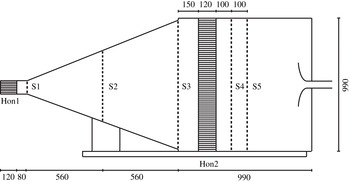
The experimental apparatus in the thermo-fluid dynamics laboratory of the University Roma TRE reproduces the free jet facility developed by Chatellier & Fitzpatrick (Reference Chatellier and Fitzpatrick2005) at the Trinity College of Dublin. The layout of the jet facility is shown in figure 1.
Layout of the experimental free jet facility. The measures are in millimetres. The abbreviation Hon# indicates the honeycomb and S# the turbulence screen.

The air is generated by a centrifugal blower which is powered by an asynchronous electric motor of about 550 W and controlled by a variable frequency inverter drive. The velocity of the jet flow is varied adjusting the inverter frequency.
The air is then sent to a wide angle diffuser through a constant section duct, which ends with a honeycomb panel and a turbulence grid (Hon1 and S1 in figure 1). The wide angle diffuser of 1120 mm length and 21° divergence angle is located upstream of the settling chamber. Two fine turbulence screens (S2 and S3 in figure 1) are installed in the middle and outlet sections of the divergent duct in order to avoid flow separation.
The
 $990~\text{mm}\times 990~\text{mm}\times 990~\text{mm}$
settling chamber consists of a straightening section made of a hexagonal honeycomb and two fine screens with the same porosity (Hon2, S4 and S5 in figure 1). The ratio of the stream-wise length to single-cell hydraulic diameter of the honeycomb as well as the porosity of the turbulence screens was designed to obtain the desired flow quality in terms of velocity profiles and turbulence intensity.
Downstream of the settling chamber the flow evolves in a nozzle which increases the flow speed. The length of the convergent duct is 210 mm, the nozzle outlet diameter is
 $D=52~\text{mm}$
and the contraction ratio is
 ${\approx}15$
.
The jet issues in a large room in order to avoid disturbances or recirculations over the jet flow.
The contraction ratio and the power of the motor enable the jet flow to achieve a maximum velocity at the nozzle exhaust (
 $U_{j}$
) of around
 $50~\text{m}~\text{s}^{-1}$
corresponding to a maximum Mach number,
 $M_{j}$
, of
 ${\approx}0.15$
. The velocity at the nozzle exhaust can be varied from
 $U_{j}=3~\text{m}~\text{s}^{-1}$
up to the maximum velocity, spanning a Reynolds number (
 $\mathit{Re}$
) range between
 $\mathit{Re}\approx 10^{4}$
and
 $\mathit{Re}=1.7\times 10^{5}$
, being
 $\mathit{Re}$
based on
 $U_{j}$
and the nozzle diameter
 $D$
.
The measurements campaign presented in the next sections were carried out at
 $U_{j}=42~\text{m}~\text{s}^{-1}$
, corresponding to
 $\mathit{Re}\approx 1.5\times 10^{5}$
, which classifies the jet as a moderate Reynolds number jet (Bogey, Marsden & Bailly Reference Bogey, Marsden and Bailly2012), and a Taylor Reynolds number
 $\mathit{Re}_{T}=\langle u^{\prime 2}\rangle ^{1/2}{\it\lambda}_{T}/{\it\nu}\cong 382$
, where
 ${\it\lambda}_{T}$
is the Taylor microscale and
 $u^{\prime }$
is the turbulent fluctuating velocity.
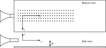
Scheme of the pin-holes distribution on the flat plate and identification of the reference system. The parameter
 $H$
represents the distance between the flat plate and the nozzle axis.

In order to pursue the objectives of the work, a rigid flat plate representing the airframe model was placed parallel to the nozzle axis. A schematic representation of the set-up and the reference frame adopted is provided in figure 2. The flat plate was installed on a rigid traverse structure facilitating the accurate positioning in the direction perpendicular to the flat plate (
 $z$
-axis). Small rotation angles are allowed along the
 $x$
and
 $y$
directions in order to align the surface to the flow direction. The size and material of the flat plate were chosen to avoid border effects and to obtain an optimal stiffness, respectively. The precise radial distance and alignment of the flat plate with respect to the nozzle axis was carefully checked using a laser levelling instrument.
2.2. Instrumentation
Several velocity and pressure measurements have been taken to characterize the jet flow quality, to investigate the aerodynamic interaction between the jet and the plate and to analyse the pressure fluctuations induced on the surface.
Velocity measurements were obtained using a single hot wire probe (DANTEC 55P11) of 1 mm in length and
 $5~{\rm\mu}\text{m}$
in diameter. The hot wire was carefully mounted with the probe stem parallel to the
 $y$
direction and in bi-normal position so as to reduce flow disturbances and provide the accurate measurement of the axial velocity component (parallel to the
 $x$
direction). The movement of the probe in the
 $z$
direction was performed by a micro-metric traversing system. The probe was connected to a constant temperature anemometer system (AN-1003 Lab-System). The velocity signals were acquired by a National Instruments acquisition system (PCI-6221). The sampling frequency was set to 100 kHz, the anti-aliasing low-pass filter frequency cut-off at 20 kHz and the acquisition time to 11 s. The frequency cut-off of the filter was chosen to maximize the resolution of the smallest scales. Anyway, it has to be pointed out that, due to the finite length of the wire, the fine-scale velocity fluctuations are attenuated. It has been estimated that probe length is 15 times larger than the Kolmogorov scale. The lack of resolution on the smallest scales affects the estimation of the local intermittency level, but not significantly the global scaling exponents.
Velocity measurements were taken both in the free jet condition and with the flat plate installed at different radial distances from the nozzle axis. More details are given in the following sections.
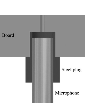
Scheme of the microphone cavity and the pin-hole. The microphone is mounted through a properly designed connector. The pinhole diameter is 1.5 mm.

Pressure fluctuations on the flat plate were measured by Microtech Gefell M360 electret microphones whose full-scale value is 134 dB and whose frequency response is flat up to 20 kHz. Microphones were cavity mounted according to the scheme reported in figure 3. The size of the cavity was designed in order to move the Helmholtz resonant peak out of the measured frequency range. An array of three microphones was used to acquire simultaneously pressure signals in the stream-wise and span-wise directions. They were positioned on the one-diameter spaced grid of points shown in figure 2. The pressure signals were acquired by a National Instruments acquisition system (SCXI-1600) with a sampling frequency set to 40 kHz, an anti-aliasing low-pass filter frequency cut-off at 20 kHz, and for an acquisition time of 10 s.
In order to characterize the overall effect of the jet flow on the wall pressure intensity, mean pressure measurements were conducted as well. The above described pin-holes were connected to a pressure transducer (Kavlico P592) through a transmission line properly designed. Mean wall pressures were acquired for 10 s with a sampling frequency of 1 kHz.
A preliminary test campaign was carried out to assess the uncertainty of all measurements. Acquisition time and sampling frequency rate were chosen to obtain a minimum confidence level of 95 % with a maximum uncertainty
 ${\it\epsilon}=2\,\%$
for all the statistical moments of interest.
2.3. Jet qualification
The jet flow qualification was carried out through hot wire velocity measurements. An in situ calibration of the probe was made before every test. The results provided profiles of the axial velocity along the
 $z$
direction for different axial distances, spanning from
 $x/D=1$
to
 $x/D=20$
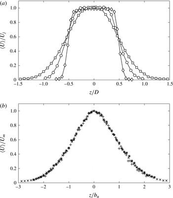
, thus covering both the jet potential core region and the fully developed turbulent region. Examples of mean velocity profiles obtained at different distances from the jet exit are shown in figure 4.
Velocity profiles along the
 $z$
-axis. (a) Velocity profiles in the potential core region normalized by the nozzle exhaust velocity: ♢
 $x/D=1$
; ○
 $x/D=3$
; ▫
 $x/D=5$
. (b) Velocity profiles in the turbulent jet region normalized by the mean velocity along the jet axis and radial distance normalized by the jet half-width:
 $\times ~x/D=10$
;
 $\ast ~x/D=15$
;
 $+~x/D=20$
.

The profiles close to the jet orifice are characterized by the well-known top hat shape, whereas in the turbulent region the typical Gaussian-like shapes are achieved. In the fully developed turbulent region a very good collapse of the self-similar profiles is found by normalizing the mean velocity amplitude (
 $\langle U\rangle$
, where the brackets denote ensemble averages) by its value on the jet axis (
 $U_{m}$
) and the radial distance by the jet half-width denoted as
 $b_{u}$
. The latter is defined as the radial distance from the axis for which the mean velocity amplitude is
 $U=0.5\,U_{m}$
.
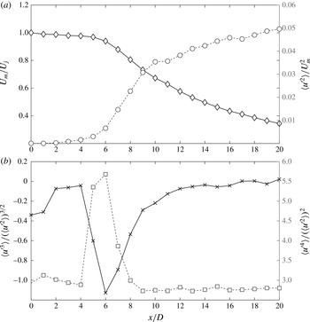
The evolution of the significant statistical quantities along the jet axis is reported in figure 5. The mean axial velocity normalized by
 $U_{j}$
and the square of the turbulence intensity relative to
 $U_{m}$
are given in 5(a). It is shown that the mean velocity remains about constant up to
 $x/D=6$
and correspondingly to this axial position the turbulence intensity starts to increase. This transition region corresponds to the end of the potential core. As pointed out in Grizzi & Camussi (Reference Grizzi and Camussi2012), the potential core length is further determined by the evolution of the skewness and kurtosis factors, which exhibit their peak values at around
 $x/D=6$
, see figure 5(b).
Evolution along the jet axis of the mean axial velocity and velocity statistic moments from the nozzle exhaust to
 $x/D=20$
. (a) Mean axial velocity normalized by the jet velocity and velocity variance normalized by the square mean velocity on the jet axis: ♢ mean velocity; ○ turbulence intensity. (b) Skewness factor and flatness factor trend:
 $\times$
skewness; ▫ flatness.

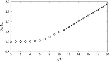
The linear fit of the centreline mean axial velocity in the fully developed flow region, represented in figure 6, provides a decay coefficient
 $K_{1}\approx 7$
, in quite good agreement with recent literature results (Or, Lam & Liu Reference Or, Lam and Liu2011). For what concerns the potential core length, an empirical model was derived by Fischer et al. (Reference Fischer, List, Koh, Imberger and Brooks1979):
 $$\begin{eqnarray}\frac{U_{m}}{U_{j}}=\frac{K_{1}}{\left(x-x_{0}\right)\!/D}=\frac{L-x_{0}}{x-x_{0}}\end{eqnarray}$$
where
 $x$
is the axial distance from the nozzle exhaust,
 $x_{0}$
is the virtual origin, which can be expressed as
 $x_{0}=K_{2}D$
, and
 $L$
is the potential core length, whose expression can be elaborated as follows:
 $$\begin{eqnarray}L=K_{1}D+K_{2}D.\end{eqnarray}$$
Inverse of the ratio between mean axial velocity and jet velocity along axial distance: ♢ potential core region; ○ transition region; ▫ developed flux region.

Antoine, Lemoine & Lebouché (Reference Antoine, Lemoine and Lebouché2001) and Uddin & Pollard (Reference Uddin and Pollard2007) found that the constant
 $K_{2}$
can also assume negative values depending on the inlet turbulence intensity. The potential core length estimated by (2.2) provides
 $L=6.6D$
, in good agreement with the present experimental results.
From the overall aerodynamic characterization the jet spreading angle evaluated by hot wire anemometer measurements was found to be close to 8°.
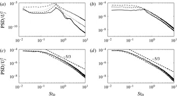
The aerodynamic characterization of the free jet is examined in more detail by calculating spectra of the fluctuating axial velocity. The evolution of the velocity power spectral density (PSD) along the jet axis is reported in figure 7 in dimensionless form. The PSD amplitudes normalized by the square of
 $U_{j}$
are represented as a function of the Strouhal number
 $\mathit{St}_{D}=f\,D/U_{j}$
. It is observed that for axial distances close to the nozzle exhaust (figure 7(a)) an energy peak at
 $\mathit{St}_{D}=0.46$
clearly emerges, this peak being the signature of the Kelvin–Helmholtz instability mode (see e.g. Danaila, Dušek & Anselmet Reference Danaila, Dušek and Anselmet1997). Higher harmonics are found in the velocity spectra for axial distances
 $x\leqslant 4D$
. As the axial distance increases the turbulence level rises as well and, in the fully developed turbulent region, all of the spectra tend to collapse and exhibit the typical Kolmogorov’s
 $f^{-5/3}$
power-law decay (Kolmogorov Reference Kolmogorov1941).
Axial evolution of dimensionless velocity PSD versus Strouhal number. (a) Solid line
 $x/D=3$
, dashed line
 $x/D=4$
, dotted line
 $x/D=5$
, dash-dotted line
 $x/D=6$
. (b) Solid line
 $x/D=7$
, dashed line
 $x/D=8$
, dotted line
 $x/D=9$
, dash-dotted line
 $x/D=10$
. (c) Solid line
 $x/D=12$
, dashed line
 $x/D=13$
, dotted line
 $x/D=14$
, dash-dotted line
 $x/D=15$
. (d) Solid line
 $x/D=17$
, dashed line
 $x/D=18$
, dotted line
 $x/D=19$
, dash-dotted line
 $x/D=20$
.

3. Results
The presence of a flat plate close to a jet flow influences significantly the overall aerodynamics. Furthermore, the impact with the surface and the subsequent near-wall tangential flow induces the generation of considerable wall pressure fluctuations. The present investigation is aimed at characterizing both the aerodynamic behaviour and the wall pressure field.
The main results achieved are reported in this section. Theoretical issues related to the wall pressure spectral modelling are also included with specific reference to classical models adopted for wall pressure fluctuations induced by fully developed turbulent boundary layers (TBLs).
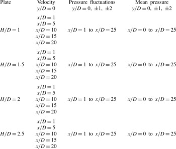
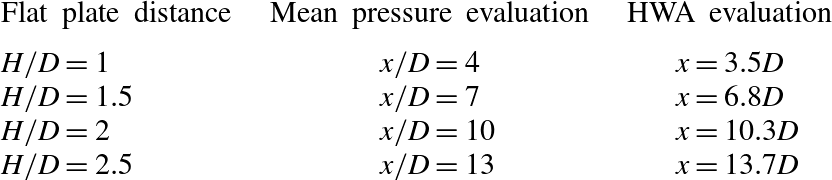
A summary of the configurations analysed and the measurements performed is given in table 1.
Summary of the experimental measurement configurations.

3.1. Velocity measurements
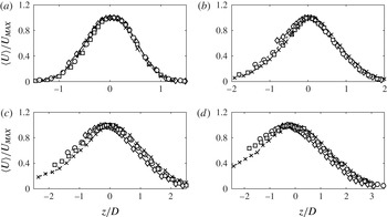
The characterization of the aerodynamic behaviour generated by the interaction of the jet plume with the flat plate is achieved by hot wire velocity measurements. As indicated in table 1, the velocity measurements were performed for four flat plate radial distances (denoted by
 $H$
) by varying the position of the probe along the
 $z$
direction within the range
 $-2.5$
to
 $-1\leqslant z/D\leqslant 4$
and from
 $x/D=1$
up to
 $x/D=20$
in the
 $x$
direction. The profiles of mean axial velocities parametrized in terms of
 $H/D$
and for different
 $x/D$
are presented in figure 8. In order to enhance the variation of the velocity profile shape induced by the presence of the rigid surface, the mean velocity is normalized with respect to its maximum (
 $U_{MAX}$
) measured along the
 $z$
direction at a fixed
 $x/D$
position. It is observed that the interaction with the flat plate influences the axisymmetry of the jet especially at large distances from the nozzle exit. The main effect induced by the plate is an increase of the mean velocity magnitude and a shift of the velocity profiles in the jet region close to the flat plate surface, i.e. for
 $z/D<0$
. It is interesting to note that the mean velocity maximum is found at
 $z/D>0$
for small
 $x/D$
, it reaches
 $z/D=0$
at about
 $x/D=10$
and, further downstream, it moves to
 $z/D<0$
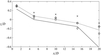
. This behaviour can be clearly observed in figure 9 where the
 $z/D$
coordinate of the velocity maximum is reported as a function of
 $x/D$
. It is shown that the
 $z$
-position where the maximum mean velocity is reached changes significantly as the axial distance increases. This means that the jet axis moves from positive radial positions to negative ones and as the plate distance from the nozzle axis increases, the transition becomes less sharp but still detectable. Furthermore, for small axial distances, i.e. very close to the nozzle exhaust, as in the case
 $x/D=1$
, the jet axis location is about constant for any distance
 $H/D$
whereas it varies significantly for larger
 $x/D$
. Such a behaviour can be associated with the jet flow evolution since the jet-plate interaction appears to be weaker in the initial part of the jet flow, close to the nozzle exhaust, and becomes more significant when the jet reaches a fully developed condition.
Velocity profiles normalized by
 $U_{MAX}$
as a function of
 $z/D$
at axial distances: (a)
 $x/D=5$
; (b)
 $x/D=10$
; (c)
 $x/D=15$
; (d)
 $x/D=20$
. Markers indicate the radial position of the flat plate with respect to the nozzle axis: ♢
 $H/D=1$
; ○
 $H/D=1.5$
; ▫
 $H/D=2$
;
 $\times ~H/D=2.5$
.

Jet axis location at different axial positions from the nozzle exhaust for different plate distances. Markers correspond to experimental results: ♢
 $H/D=1$
;○
 $H/D=1.5$
; ▫
 $H/D=2$
;
 $\times ~H/D=2.5$
. Lines correspond to the numerical trend obtained by CFD RANS: solid line
 $H/D=1.5$
, dashed line
 $H/D=2.5$
.

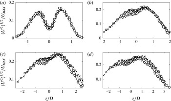
The relative turbulence intensity as a function of the radial position is represented in figure 10. The velocity standard deviation is divided by
 $U_{MAX}$
and parametrized as in figure 8. In all cases, the presence of the rigid surface induces an asymmetry of the turbulence profiles, the maximum being moved towards the side of the jet opposite to the plate position. Unlike the mean aerodynamic field, the effects on the fluctuating velocity field observed in the experiments were compared with numerical data found in the literature. The results achieved in the present work are in good agreement with the turbulence evolution provided by Smith & Miller (Reference Smith and Miller2013).
Turbulence intensity profiles as a function of
 $z/D$
at axial distances: (a)
 $x/D=5$
; (b)
 $x/D=10$
; (c)
 $x/D=15$
; (d)
 $x/D=20$
. Markers indicate the radial position of the flat plate with respect to the nozzle axis: ♢
 $H/D=1$
; ○
 $H/D=1.5$
; ▫
 $H/D=2$
;
 $\times ~H/D=2.5$
.

Neither experimental nor numerical data can be found in literature to compare the effects due to jet–surface interaction on the mean velocity field. Hence, in order to verify qualitatively the trend found in the experiments, a numerical three-dimensional simulation has been carried out through a standard RANS approach. The latest generation of RANS models is able to accurately predict aerodynamic changes in the mean field variables.
The simulations reproduce the same geometric set-up, flow conditions and ambient conditions of the present experiment, but the plate was positioned at only two radial distances from the nozzle axis:
 $H/D=1.5$
and
 $H/D=2.5$
.
The simulation was performed using the software Fluent
© and adopting a standard
 $k{-}{\it\epsilon}$
turbulence model. Several meshes have been tested through a mesh sensitivity analysis. The adopted one consisted of 3 million cells non-uniformly distributed in order to reasonably well resolve the region close to the flat plate surface overflown by the jet flow.
For the sake of conciseness the numerical results are not presented herein, except for the estimation of the maximum velocity location that is reported in figure 9 together with the experimental outcomes. Even though qualitatively, the numerical results confirm the shift of the jet axis location as a function of the axial distance from the nozzle exhaust; it is also confirmed that for the plate position closer to the jet, the transition is faster and sharper. It can be observed that the trend of the jet axis shift along the axial distance is qualitatively the same between the experimental and numerical results.
3.2. Pressure measurements
As pointed out in 2.2, a well-detailed description of the fluctuating pressure field on the flat plate surface for different radial positions is provided. Wall pressure measurements were performed with an array of three one-diameter spaced microphones. The pressure evolution was studied both in the stream-wise direction, from
 $x/D=0$
to
 $x/D=25$
, and in the span-wise direction, from
 $y/D=-2$
to
 $y/D=2$
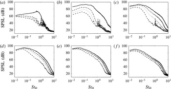
. Figure 11 shows the sound pressure spectrum level (SPSL) defined, according to Pierce (Reference Pierce1989), as follows:
 $$\begin{eqnarray}\text{SPSL}=10\hspace{2.22198pt}\log _{10}\left(\frac{{p_{f}}^{2}(\,f)\left({\rm\Delta}f\right)_{ref}}{p_{ref}^{2}}\right)\end{eqnarray}$$
where
 ${p_{f}}^{2}(\,f)$
is the PSD function,
 $f$
is the frequency,
 ${\rm\Delta}f_{ref}$
is the reference bandwidth (1 Hz) and
 $p_{ref}$
the reference pressure (
 $20~{\rm\mu}\text{Pa}$
). The SPSLs are plotted as a function of the Strouhal number
 $\mathit{St}_{D}$
for each plate distance and for a set of axial positions along the nozzle axis ranging from
 $x=1D$
to
 $25D$
.
SPSL versus Strouhal number at axial distances: (a)
 $x/D=1$
; (b)
 $x/D=5$
; (c)
 $x/D=10$
; (d)
 $x/D=15$
; (e)
 $x/D=20$
; (f)
 $x/D=25$
. For flat plate positions: solid line
 $H/D=1$
; dashed line
 $H/D=1.5$
; dotted line
 $H/D=2$
; dash-dotted line
 $H/D=2.5$
.

The pressure fluctuation intensity and the spectral shape in figure 11 change significantly as the jet–flat plate separation distance decreases. Such a behaviour is particularly detectable for small axial distances where the spectra show a higher energy content over the whole frequency range. It has to be pointed out that the peaks emerging in the spectra for
 $\mathit{St}_{D}>1$
for the large
 $H/D$
are related to the background noise and have no physical meaning.
As the axial distance increases, the energy of the fluctuating pressure increases and the shape of the spectra changes accordingly. This is due to the relationship between the radial position of the plate and the axial location where the jet hits the surface. Also the wall pressure statistics changes significantly if the impact occurs correspondingly to the potential core region, the transition region or the fully developed region. A quasi-equilibrium TBL on the surface can be established only at large distances from the impact region, this behaviour being again related to the radial position of the flat plate.
An overall picture of the wall pressure evolution is given in figure 12, where the time-averaged pressure coefficient and the root-mean-square pressure coefficient along the jet axis are reported. The pressure coefficients are respectively defined as follows:
 $$\begin{eqnarray}\displaystyle & \displaystyle c_{p}=\frac{\langle p\rangle -p_{amb}}{{\textstyle \frac{1}{2}}{\it\rho}\,U_{j}^{2}} & \displaystyle\end{eqnarray}$$
 $$\begin{eqnarray}\displaystyle & \displaystyle c_{p_{rms}}=\frac{p_{rms}}{{\textstyle \frac{1}{2}}{\it\rho}\,U_{j}^{2}} & \displaystyle\end{eqnarray}$$
 $\langle p\rangle$
and
 $p_{rms}$
are the ensemble average of the transducer pressure signals and the root mean square of the microphone pressure signals, respectively. Here,
 $p_{amb}$
and
 ${\it\rho}$
are respectively the ambient pressure and density. It has to be pointed out that the
 $p_{rms}$
coincides with standard deviation of the pressure as the microphone signal has zero mean.
(a) Mean pressure coefficient on the flat plate along the jet axis; (b) root-mean-square pressure coefficient on the surface along the jet axis. For flat plate positions: ♢
 $H/D=1$
; ○
 $H/D=1.5$
; ▫
 $H/D=2$
;
 $\times ~H/D=2.5$
.

The trend is different depending on jet–flat plate separation distances, but some analogies are found.
Except for the largest
 $H/D$
, three regions can be identified.
-
(i) First region: the mean pressure coefficient remains about constant and the
 $c_{p_{rms}}$
increases.
-
(ii) Second region: the mean pressure coefficient increases reaching its maximum and the
$c_{p_{rms}}$
remains about constant. -
(iii) Third region: the mean pressure coefficient and the
$c_{p_{rms}}$
both decay slowly. The mean pressure recovers almost the initial amplitude, whereas the pressure fluctuations remain larger as an effect of the development of a boundary layer.


The different behaviour observed for the largest
 $H/D$
can be ascribed to the fact that in this configuration the plate is quite far from the jet and the jet impact occurs far from the nozzle exhaust, approximately around
 $x/D=13$
. At such a distance, the jet can be considered fully turbulent, as its mean kinetic energy is much lower than that in the region closer to the jet orifice. It is reasonable to suppose that the beginning of the second region corresponds approximately to the point where the jet flow impacts the plate. This idea is supported by the results reported in table 2. Here, the position of the impact estimated by the measured spreading angle of the jet is compared with the positions where the mean pressure coefficient starts to rise. As it can be observed, a very good agreement between the two estimations is found.
Summary of the jet impact axial positions on the flat plate surface.

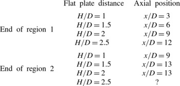
Table 3 clarifies and summarizes the distinction between the three regions described above. Except for the case
 $H/D=2.5$
, where it is not possible to clearly detect the end of region 2, the separation between the three regions appears reasonable.
Axial locations of the jet–flat plate surface interaction regions.

The SPSLs obtained in the span-wise direction for axial distances
 $x/D=15$
and
 $x/D=25$
and for each flat plate separation distance are presented in figures 13 and 14. The transverse positions
 $y/D=0,1,2$
are considered. For
 $x/D=15$
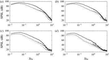
the difference between each transverse location is more significant: the spectra for
 $y/D=0$
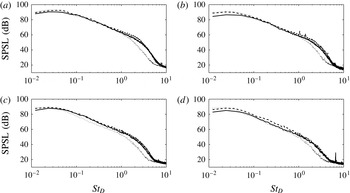
show a higher amplitude especially in the middle-frequency range. As the span-wise distance increases the spectral energy decreases and the peaks related to the background noise emerge. For large axial distances, i.e. in the fully turbulent jet region, the spectra collapse in the low- and mid-frequency range and exhibit a steeper energy decay in the high-frequency range as the transverse distance increases.
SPSL versus Strouhal number along the span-wise direction for
 $x/D=15$
. Flat plate positions: (a)
 $H/D=1$
; (b)
 $H/D=1.5$
; (c)
 $H/D=2$
; (d)
 $H/D=2.5$
. Transversal locations: solid line
 $y/D=0$
; dashed line
 $y/D=1$
; dotted line
 $y/D=2$
.

SPSL versus Strouhal number along the span-wise direction for
 $x/D=25$
. Flat plate positions: (a)
 $H/D=1$
; (b)
 $H/D=1.5$
; (c)
 $H/D=2$
; (d)
 $H/D=2.5$
. Transversal locations: solid line
 $y/D=0$
; dashed line
 $y/D=1$
; dotted line
 $y/D=2$
.

In order to have a global picture of the fluctuating pressure field, the overall sound pressure level (OASPL) has been computed in each axial and transverse location and for each
 $H/D$
. The OASPL is defined as follows:
 $$\begin{eqnarray}\text{OASPL}=20\log _{10}\frac{{\it\sigma}_{p}}{p_{ref}}\end{eqnarray}$$
where
 ${\it\sigma}_{p}$
is the pressure standard deviation.
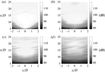
The OASPL contour maps are reported in figure 15. It can be noticed that the closer is the position of the flat plate the higher is the OASPL over the whole surface. The pressure footprint is clearly observed closely downstream of the nozzle exit for
 $H/D=1$
. As the flat plate separation distance increases, the pressure footprint becomes weaker and the axial position where the maximum noise level is found moves further downstream. In the region of the surface corresponding to the fully turbulent jet the OASPL variation along the transverse direction reduces significantly.
OASPL map on the flat plate at distances: (a)
 $H/D=1$
; (b)
 $H/D=1.5$
;(c)
 $H/D=2$
; (d)
 $H/D=2.5$
.

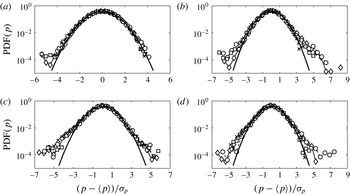
The wall pressure statistics are also studied in terms of probability density function (PDF) distributions. The comparisons of the PDF distributions are presented in figure 16 for different
 $H/D$
and axial distances. The pressure variable is expressed in reduced form, i.e. normalized in order to have zero mean value and unit standard deviation. PDFs achieved from the experiments are compared with the normal Gaussian distribution. All of the pressure distributions deviate from the Gaussian one, such discrepancy becoming more significant as the axial distance increases. The positive skewness observed for
 $x/D=10$
at
 $H/D=1$
,
 $H/D=1.5$
and
 $H/D=2$
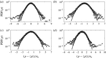
can be ascribed to the intermittent large-amplitude velocity fluctuations induced by the jet flow structures that impact on the flat plate surface and evolve over it. Additional experiments with flow visualization techniques are planned to confirm this hypothesis. Another aspect which has to be pointed out is that for increasing axial distances, the PDF tails become higher than the Gaussian distribution. This behaviour is more evident in figure 17, where the axial evolution of the PDFs is given in terms of
 $x/D$
and for all of the
 $H/D$
considered. The PDF tails follow an exponential evolution as the
 $x/D$
position increases, a typical behaviour in fully developed turbulence (Tsuji et al.
Reference Tsuji, Fransson, Alfredsson and Johansson2007).
Pressure PDF at axial positions: (a)
 $x/D=3$
; (b)
 $x/D=10$
; (c)
 $x/D=17$
; (d)
 $x/D=24$
. Flat plate positions: ♢
 $H/D=1$
; ○
 $H/D=1.5$
; ▫
 $H/D=2$
;
 $\times ~H=2.5D$
.

Axial evolution of the pressure PDF at plate positions: (a)
 $H/D=1$
;(b)
 $H/D=1.5$
; (c)
 $H/D=2$
; (d)
 $H/D=2.5$
. Axial locations: ♢
 $x/D=2$
; ○
 $x/D=6$
; ▫
 $x/D=10$
;
 $\times ~x/D=14$
;
 $+~x/D=18$
;
 $\unicode[STIX]{x2B21}$
 $x/D=23$
.

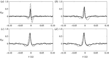
Wall pressure statistics are investigated in the time domain through the cross-correlation function computed between two contiguous microphones. The cross-correlation is defined as
 $$\begin{eqnarray}R_{pp}\left({\it\xi},{\it\tau}\right)=\langle p\left(x,t\right),\,p\left(x+{\it\xi},t+{\it\tau}\right)\rangle\end{eqnarray}$$
where
 ${\it\xi}$
is the distance between microphones (in the present study
 ${\it\xi}=1D$
),
 ${\it\tau}$
is the time lag and the symbol
 $\langle \,\rangle$
denotes ensemble averages. The cross-correlation coefficient
 ${\it\rho}_{pp}$
, obtained normalizing the cross-correlation function by the pressure covariance, is plotted in figure 18 for different
 $H/D$
and axial positions. For axial distances close to the nozzle exhaust
 ${\it\rho}_{pp}$
is always asymmetric. On the other hand, as the jet becomes completely turbulent, the cross-correlation shape becomes symmetric. Furthermore, flow structures of larger size convected through the flow cause the cross-correlation coefficient to become wider as
 $H/D$
increases. Thus, the jet–flat plate interaction has the effect to break the large turbulent structures as the plate approaches to the jet. This result is in agreement with the turbulence intensity profiles reported in figure 10, in which a decrease of turbulence occurs in the jet region close to the flat plate.
Wall pressure cross-correlation coefficient on the jet axis at axial positions: (a)
 $x/D=8$
; (b)
 $x/D=14$
; (c)
 $x/D=20$
; (d)
 $x/D=24$
. Flat plate positions: solid line
 $H/D=1$
; dashed line
 $H/D=1.5$
; dotted line
 $H/D=2$
; dash-dotted line
 $H/D=2.5$
.

Cross-correlations were exploited to evaluate the convection velocity (
 $U_{c}$
) along the jet axis.
 $U_{c}$
is determined as the ratio between the microphone distance
 ${\it\xi}$
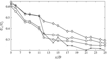
and the time lag at which the cross-correlation maximum is detected. The convection velocity as a function of the stream-wise position along the jet axis is reported in figure 19. The value found in the potential core region is in good agreement with the literature results i.e.
 $U_{c}\approx 0.6\,U_{j}$
(Picard & Delville Reference Picard and Delville2000). As the axial distance increases, and the jet mean velocity decreases, the convection velocity decreases as well, reaching
 $U_{c}/U_{j}\approx 0.25$
for very large
 $x/D$
. A significant dependence of
 $U_{c}$
upon
 $H$
is observed for large
 $x/D$
, whereas at small distances from the jet a more universal behaviour is detected.
Convection velocity along the stream-wise direction on the jet axis at positions: ♢
 $H/D=1$
; ○
 $H/D=1.5$
; ▫
 $H/D=2$
;
 $\times ~H/D=2.5$
.

3.2.1. Spectral modelling
As was shown in figure 11, the amplitude and shape of the wall pressure auto-spectra depend significantly upon the flat plate distance and the axial position of the microphone with respect to the jet exit. For large
 $x/D$
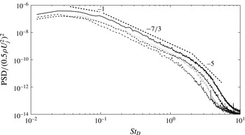
, where the jet has completely developed on the flat plate, a more universal trend can be found as an effect of the development of a TBL over the wall (Hwang, Bonness & Hambric Reference Hwang, Bonness and Hambric2009). Figure 20 shows the spectra for all
 $H/D$
determined at an axial distance of
 $x/D=25$
. A slope
 $\propto f^{-1}$
is found in the frequency range immediately after the spectrum peak, according to the energy decay law commonly observed in the overlap region for fully developed TBL wall pressure spectra. In the mid-frequency range an energy decay power law
 $\propto f^{-7/3}$
, typical of fully turbulent flows, is observed. In the high-frequency range, the spectral shape is affected by viscosity and a power law decay close to
 $f^{-5}$
is found.
Dimensionless PSDs of wall pressure signals at axial distance
 $x/D=25$
. For flat plate positions: solid line
 $H/D=1$
; dashed line
 $H/D=1.5$
; dotted line
 $H/D=2$
; dash-dotted line
 $H/D=2.5$
.

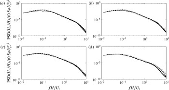
A unique scaling criterion able to lead all of the spectra to collapse cannot be found due to the spectra shape dependence on the different geometrical configurations considered. For positions far from the jet exit a scaling criterion is proposed using external aerodynamic variables,
 $H$
and
 $U_{j}$
, as reference length and velocity scales, respectively. The typical time scale to be used is related to the time occurring to a fluid particle advected by the mean flow to reach the flat plate. Therefore, it is estimated by the ratio
 $H/U_{c}$
being
 $U_{c}$
the convection velocity determined in § 3.2. Accordingly, the PSDs and the frequency are normalized as follows:
 $$\begin{eqnarray}\displaystyle & \displaystyle \text{PSD}_{scaled}=\frac{\text{PSD}}{\left(0.5{\it\rho}\,U_{c}^{2}\right)^{2}\,{\displaystyle \frac{H}{U_{c}}}} & \displaystyle\end{eqnarray}$$
 $$\begin{eqnarray}\displaystyle & \displaystyle \mathit{St}_{H}=\frac{f\,H}{U_{j}}. & \displaystyle\end{eqnarray}$$
The normalization was applied to auto-spectra at different axial locations and flat plate distances, but, as pointed out above, a satisfactory collapse of the spectra is achieved only far from the nozzle exhaust.
As shown in figure 21, according to the definitions given in table 3, a satisfactory collapse was found for spectra corresponding to positions at the end of region 2 and in different axial positions in the region 3. The results of figure 21 suggest that once the jet flow has impacted the wall, the wall pressure auto-spectra become universal, this behaviour occurring before a fully developed TBL is reached.
Scaled wall pressure spectra at different axial positions and flat plate distances depending on the region of table 3. Solid lines
 $H/D=1$
: (a)
 $x/D=8$
;(b)
 $x/D=12$
; (c)
 $x/D=14$
; (d)
 $x/D=18$
. Dashed lines
 $H/D=1.5$
: (a)
 $x/D=12$
;(b)
 $x/D=14$
; (c)
 $x/D=18$
; (d)
 $x/D=24$
. Dash-dotted lines
 $H/D=2$
: (a)
 $x/D=13$
; (b)
 $x/D=15$
; (c)
 $x/D=18$
; (d)
 $x/D=24$
. Dotted lines
 $H/D=2.5$
: (a)
 $x/D=18$
;(b)
 $x/D=22$
; (c)
 $x/D=24$
; (d)
 $x/D=25$
.

Similar conclusions can be addressed by the analysis of the coherence function determined along the jet axis and evaluated as follows (Di Marco et al. Reference Di Marco, Camussi, Bernardini and Pirozzoli2013):
 $$\begin{eqnarray}{\it\gamma}\left({\it\xi},{\it\omega}\right)=\frac{|{\it\Phi}_{p_{1}p_{2}}\left({\it\xi},{\it\omega}\right)\!|}{\left[{\it\Phi}_{p_{1}}\left({\it\omega}\right){\it\Phi}_{p_{2}}\left({\it\omega}\right)\right]^{1/2}}\end{eqnarray}$$
where
 ${\it\omega}$
is the angular frequency,
 ${\it\Phi}_{p_{1}p_{2}}$
the cross-spectrum,
 ${\it\Phi}_{p_{1}}$
and
 ${\it\Phi}_{p_{2}}$
the auto-spectra of two consecutive microphones separated in the streamwise direction by
 ${\it\xi}=1D$
. Based on the results summarized in table 2, the coherence function was calculated beyond the axial positions where the jet impacts the flat plate. Experimental results were compared with the Corcos’ model formulation (Finnveden et al.
Reference Finnveden, Birgersson, Ross and Kremer2005) providing a prediction of the coherence function that is defined as follows:
 $$\begin{eqnarray}{\it\gamma}\left({\it\xi},{\it\omega}\right)=\exp \left(-{\it\alpha}\frac{{\it\omega}\,{\it\xi}}{U_{c}}\right)\end{eqnarray}$$
where the constant
 ${\it\alpha}$
was empirically determined by a least mean square optimization algorithm.
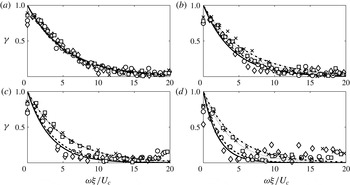
The coherence spectra versus the normalized angular frequency
 ${\it\omega}\,{\it\xi}/U_{c}$
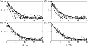
(Farabee & Casarella Reference Farabee and Casarella1991) are shown in figure 22 for all
 $H/D$
and at axial distances
 $x/D\geqslant 14$
. The exponential decay along the normalized frequency typical of the Corcos’ formulation is well reproduced by the experiments. For small axial distances a small discrepancy of the experimental data with respect to the Corcos’ model is found as the distance
 $H/D$
increases. Moving downstream in the jet and thus approaching a developed TBL, the experimental points become less scattered for all of the flat plate distances. This behaviour is confirmed by figure 23, which shows the axial evolution along the nozzle axis of the coherence function for all
 $H/D$
. It can be observed that the exponential decay is well reproduced, but the decay coefficient decreases for increasing distances
 $x/D$
.
Coherence function parametrized by the flat plate distance for axial positions: (a)
 $x/D=14{-}15$
; (b)
 $x/D=17{-}18$
; (c)
 $x/D=21{-}22$
; (d)
 $x/D=24{-}25$
. Markers are for experimental data and lines for Corcos’ model fits: diamonds and solid line
 $H/D=1$
; circles and dashed line
 $H/D=1.5$
; squares and dotted line
 $H/D=2$
; crosses and dash-dotted line
 $H/D=2.5$
.

Stream-wise evolution of the coherence function for flat plate distances: (a)
 $H/D=1$
; (b)
 $H/D=1.5$
; (c)
 $H/D=2$
; (d)
 $H/D=2.5$
. Markers are for experimental data and lines for Corcos’ model fits: diamonds and solid line
 $x/D=14{-}15$
; circles and dashed line
 $x/D=17{-}18$
; squares and dotted line
 $x/D=21{-}22$
; crosses and dash-dotted line
 $x/D=24{-}25$
.

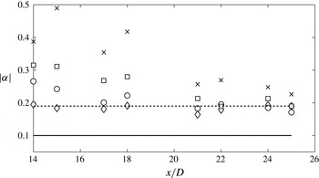
Figure 24 summarizes the axial evolution of the Corcos’ coefficient
 ${\it\alpha}$
for all
 $H/D$
. Values of
 ${\it\alpha}$
ranging from 0.1 to 0.19, found in literature (see, e.g., Bull Reference Bull1967; Brooks & Hodgson Reference Brooks and Hodgson1981) are also reported. For the smallest
 $H/D$
it is found
 $|{\it\alpha}|\simeq 0.2$
for all of the considered axial positions, which is surprisingly in very good agreement with the amplitude reported in the literature for equilibrium TBLs. At larger
 $H/D$
, the measured Corcos’ coefficients are higher than those found in literature. The larger is
 $H/D$
the larger is the coefficient, but for increasing
 $x/D$
the amplitude of
 $|{\it\alpha}|$
decreases and the tendency is to reproduce again the amplitude 0.2, expected for equilibrium TBL.
Axial evolution of the Corcos’ model stream-wise coefficient from
 $x/D=14$
to
 $x/D=25$
for flat plate distances: ♢
 $H/D=1$
; ○
 $H/D=1.5$
; ▫
 $H/D=2$
;
 $\times ~H/D=2.5$
. Solid line and dashed line refer respectively to the lower and upper limit values of the Corcos’ model coefficient.

4. Conclusions
The interaction between an incompressible moderate Reynolds number jet and a flat plate parallel to the nozzle axis has been investigated experimentally through velocity and wall pressure measurements carried out for different radial distances of the rigid surface from the nozzle axis. The core of the work is focused on the analysis of the wall pressure fluctuations induced by the tangential jet flow, an issue that has never been studied before neither experimentally nor numerically.
The values of the mean and fluctuating velocity field, needed to characterize the free jet aerodynamics, were first obtained as a function of the downstream position (
 $x/D$
) and transverse position (
 $z/D$
) of a hot wire probe.
The next step was to investigate the effect of a parallel flat plate at various radial distances (
 $H/D$
) on the aerodynamic fields through velocity measurements. Results show that both the mean and the fluctuating aerodynamic field are affected by the presence of the flat plate, which induces a positive or negative shift in
 $z$
direction of the velocity and turbulence intensity profiles. Positive shifts of the mean velocity profiles are found at downstream positions close to the nozzle exit; as the axial distance increases, the velocity profiles moved towards the plate (negative shift). Such a behaviour results in a change of the jet axis position which was defined by the radial location where the maximum velocity value was measured. It depends both on the considered axial position and the flat plate distance. For what concern turbulence intensities the profiles are shifted in the positive direction. Velocity fluctuations lower than the ones corresponding to the free jet configuration are found in the region close to the flat plate (
 $z/D<0$
). The effect of the flat plate was to break the large structures impacting on the surface.
Pressure fluctuation signals on the flat plate were acquired by an array of three cavity mounted microphones moved over a grid of points which spans 25
 $D$
in the stream-wise direction and 5
 $D$
in the span-wise direction. Pressure measurement results show that the energy content and the spectral shape changes significantly for different stream-wise locations. Moreover, for a given axial position, the auto-spectra are very different depending on the flat plate distance. As the axial distance increases and the jet impact on the flat plate has occurred, spectra show higher energy contents. Far downstream of the jet nozzle exhaust, the pressure spectra show a self-similar shape and energy decay laws typical of TBL wall pressure can be applied.
In the span-wise direction, large differences in terms of amplitude and spectral shape are found at axial positions close to the nozzle exhaust. As the transverse distance from the nozzle axis increases the energy content decreases. In the fully developed jet region, the spectra in the span-wise direction become very similar and collapse. A global description of the fluctuating pressure field on the flat plate is given by the OASPL contour map on the surface. The OASPL map confirms the development in the stream-wise and span-wise direction illustrated above.
For what concerns the axial evolution of the wall pressure field, three regions are detected based on the mean and root mean square pressure distribution over the flat plate surface. (i) The first region: the jet has not yet impacted on the flat plate surface and the spectra energy content is weak. (ii) The second region: the jet has impacted on the flat plate surface. The mean pressure increases, although the root-mean-square pressure is almost constant. The axial position of the jet impact derived from the mean pressure distribution is confirmed by the impact point obtained from the jet spreading angle evaluated by hot wire measurements. (iii) The third region: the mean pressure decreases with oscillations which could be related to the large structures convected by the jet flow over the flat plate surface after the impact region. This region represents a transition to a quasi-equilibrium TBL. This thesis is confirmed by the energy decay laws of the pressure spectra, typical of TBL wall pressure spectra, found at large axial positions and for all the flat-plate distances from the nozzle axis.
Basic issues useful for the wall pressure spectral modelling have also been addressed. A scaling criterion for pressure auto-spectra based on global aerodynamic quantities is derived for region 2 and region 3. The scaling law is based on the convection velocity, the flat plate distance from the nozzle axis and the mean jet velocity at the nozzle exhaust. The collapse of the normalized spectra is quite satisfactory.
The coherence function along the stream-wise direction is computed for axial locations beyond the impact zone over the surface and for all of the flat plate distances. Experimental results are compared with the Corcos’ model prediction. The experimental data satisfy the exponential decay within the frequency range typical of the Corcos’ formulation. For the smallest
 $H/D$
the value of the empirical Corcos’ coefficient
 $|{\it\alpha}|$
of the exponential fit is within the range found in the literature for all of the axial positions analysed. At larger flat plate distances and for small axial positions,
 $|{\it\alpha}|$
is slightly larger than the expected one. In any case, for increasing distances from the nozzle exhaust, the wall flow develops towards a fully developed TBL and the coefficient value tends to that formulated by Corcos.
Acknowledgements
The authors acknowledge the partial support of the EU Collaborative project JERONIMO (ACP2-GA-2012-314692), funded under the 7th Framework Program. G. Lior is acknowledged for his help during the measurement campaign.