1 Introduction
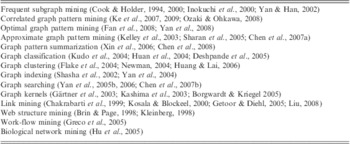
The primary goal of data mining is to extract statistically significant and useful knowledge from data (Chen et al., Reference Chen, Han and Yu1996; Han & Kamber, 2006). The data of interest can take many forms: vectors, tables, texts, images, and so on. Data can also be represented by various means. Structured data and semi-structured data are naturally suited to graph representations. To give one example, if we consider protein–protein interaction networks (a common application area for graph mining), these can be represented in a graph format such that the vertexes indicate genes, and the directed or undirected edges indicate physical interactions or functional associations (Alm & Arkin, Reference Alm and Arkin2003). Because of the ease with which structured and semi-structured data can be represented in graph formats, there has been much interest in the mining of graph data (often referred to as graph-based data mining or graph mining). A number of popular research sub-domains of graph mining are listed in Table 1.
Popular graph mining research sub-domains

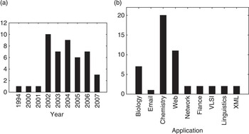
Frequent subgraph mining (FSM) is the essence of graph mining. The objective of FSM is to extract all the frequent subgraphs, in a given data set, whose occurrence counts are above a specified threshold. Figure 1 presents an overview of the domain of FSM in terms of the number of significant FSM algorithms that have been proposed over the period 1994 to the present. From the figure, we can see periods of activity in the early 90s (coinciding with the introduction of the concept of data mining), followed by another period of activity from 2002 to 2007. No ‘new’ algorithms have been introduced over the past few years, indicating that the field is reaching maturity, although there has been much work focused on variations of existing algorithms.
The distribution of the most significant FSM algorithms with respect to the year of introduction and application domain

Other than the research activity associated with FSM, the importance of FSM is also reflected in its many areas of its application. Figure 1b presents an overview of the application domain of FSM in terms of the number of FSM algorithms reported in the literature and the specific application domain at which they have been directed. From the figure, it can be seen that three application domains (chemistry, web, and biology) dominated the usage of FSM algorithms.
The straightforward idea behind FSM is to ‘grow’ candidate subgraphs, in either a breadth-first or depth-first manner (candidate generation), and then determine whether the identified candidate subgraphs occur frequently enough in the graph data set for them to be considered interesting (support counting). Thus, the two main research issues in FSM are how to efficiently and effectively (i) generate the candidate frequent subgraphs and (ii) determine the frequency of occurrence of the generated subgraphs. Effective candidate subgraph generation requires that the generation of duplicate or superfluous candidates is avoided. Occurrence counting requires repeated comparison of candidate subgraphs with subgraphs in the input data, a process known as isomorphism checking. FSM, in many respects, can be viewed as an extension of Frequent Itemset Mining (FIM) popularized in the context of Association Rule Mining (ARM; see e.g. Agrawal & Srikant, Reference Agrawal and Srikant1994). Consequently, many of the proposed solutions to addressing the main research issues effecting FSM are based on similar techniques found in the domain of FIM. For example, the downward closure property (DCP) associated with itemsets has been widely adopted with respect to candidate subgraph generation.
In this paper, the authors present a survey of the current ‘state of the art’ of FSM. With reference to the literature, we can identify many different types of mining strategies, with respect to many different types of graph, to produce many different kinds of patterns. So as to impose some form of order to the domain of FSM, we have focused on the nature of FSM algorithms, categorizing such algorithms according to: (i) candidate generation strategy, (ii) the mechanism for traversing the search space, and (iii) the occurrence counting process. To further facilitate understanding of the field of FSM, we distinguish between frequent subtree mining and the much general domain of FSM. The rest of this paper is organized as follows. We begin in Section 2 by introducing some formal definitions and terminology, followed in Section 3 with a generic overview of the FSM process. In Sections 4 and 5, we then consider current frequent subtree and subgraph mining algorithms, respectively. A brief summary is provided at the end of both the sections. Finally, Section 6 presents some conclusions and future directions.
2 Formalism
There are two separate problem formulations for FSM: (i) graph transaction-based FSM and (ii) single graph-based FSM. In graph transaction-based FSM, the input data comprise a collection of medium-size graphs called transactions. Note that the term ‘transaction’ is borrowed from the field of ARM (Agrawal & Srikant, Reference Agrawal and Srikant1994). In single graph-based FSM the input data, as the name implies, comprise one very large graph.
A subgraph g is considered to be frequent if its occurrence count is greater than some predefined threshold value. The occurrence count for a subgraph is usually referred to as its support, and consequently the threshold is referred to as the support threshold. The support of g may be computed using either transaction-based counting or occurrence-based counting. Transaction-based counting is only applicable to graph transaction-based FSM, while occurrence-based counting may be applied to either transaction-based FSM or single graph-based FSM. However, occurrence-based counting is typically used with single graph-based FSM.
In transaction-based counting the support is defined by the number of graph transactions that g occurs in, one count per transaction regardless of whether g occurs once or more than once in a particular graph transaction. Thus, given a database  $$\[--><$> {\scr G}\, = \,{\rm{\{ }}{{G}_1},{{G}_2},\, \ldots, \,{{G}_T}{\rm{\} }} <$><!--$$ consisting of a collection of graph transactions, and a support threshold σ (0 < σ ⩽ 1); then the set of graph transactions where a subgraph g occurs is defined by
 $$\[--><$> {{\delta }_{\scr G}}{\rm{(}}g{\rm{)}}\, = \,{\rm{\{ }}{{G}_i}|g\, \subseteq \,{{G}_i}{\rm{\} }} <$><!--$$. Thus, the support of g is defined as
 $$su{{p}_{\scr G}}{\rm{(}}g{\rm{)}}\, = \,|{{\delta }_{\scr G}}{\rm{(}}g{\rm{)}}|/T$$
where  $$\[--><$> |{{\delta }_{\scr G}}{\rm{(}}g{\rm{)}}| <$><!--$$ denotes the cardinality of
 $$\[--><$> {{\delta }_{\scr G}}{\rm{(}}g{\rm{)}} <$><!--$$, and T the number of graphs (transactions) in G. Therefore, g is frequent if and only if
 $$\[--><$> su{{p}_{\scr G}}{\rm{(}}g{\rm{)}}\,{\geqslant}\,\sigma <$><!--$$. In occurrence-based counting, we simply count up the number of occurrences of g in the input set.
Transaction-based counting offers the advantage that the well-known DCP Footnote 1 can be employed to significantly reduce the computation overhead associated with candidate generation in FSM. In the case of occurrence-based counting, either an alternative frequency measure, which maintains the DC property, must be established or some heuristics adopted to keep the computation as inexpensive as possible. There are a variety of support measures (Vanetik, Reference Vanetik2002; Kuramochi & Karypis, Reference Kuramochi and Karypis2004c, Reference Kuramochi and Karypis2005; Vanetik et al., Reference Vanetik, Shimony and Gudes2006) that may be adopted for single graph-based FSM, these will be discussed further in Subsection 5.1.2.
2.1 Preliminary definitions
Generally speaking, a graph is defined to be a set of vertexes (nodes), which are interconnected by a set of edges (links) (Gibbons, Reference Gibbons1985). The graphs used in FSM are assumed to be labelled simple graphs Footnote 2. In the following paragraphs, a number of widely used definitions, used later in this paper, are introduced.
Labelled graph: A labelled graph can be represented as G(V, E, LV, LE, ϕ), where V is a set of vertexes, E ⊆ V × V is a set of edges; LV and LE are sets of vertex and edge labels, respectively; and ϕ is a label function that defines the mappings V → LV and E → LE. G is (un)directed if ∀e ∈ E, e is an (un)ordered pair of vertexes. A path in G is a sequence of vertexes that can be ordered such that two vertexes form an edge if and only if they are consecutive in the list (West, Reference West2000). G is connected, if it contains a path for every pair of vertexes in it and disconnected otherwise. G is complete if each pair of vertexes is joined by an edge, and G is acyclic if it contains no cycle.
Subgraph: Given two graphs
 $$\[--><$> {{G}_1}{\rm{(}}{{V}_1},{{E}_1},{{L}_{{{V}_1}}},{{L}_{{{E}_1}}},{{\varphi }_1}{\rm{)}} <$><!--$$ and $$\[--><$> {{G}_2}{\rm{(}}{{V}_2},{{E}_2},{{L}_{{{V}_2}}},{{L}_{{{E}_2}}},{{\varphi }_2}{\rm{)}} <$><!--$$, G 1 is a subgraph of G 2, if G 1 satisfies: (i) $$\[--><$> {{V}_1}\, \subseteq \,{{V}_2}\,\,{\rm{and}}\,\,\forall v\, \in \,{{V}_1},{{\varphi }_1}{\rm{(}}v{\rm{)}}\, = \,{{\varphi }_2}{\rm{(}}v{\rm{)}} <$><!--$$ and (ii) $$\[--><$> {{E}_1}\, \subseteq \,{{E}_2}\,{\rm{and}}\,\forall {\rm{(}}u,v{\rm{)}}\, \in \,{{E}_1},{{\varphi }_1}{\rm{(}}u,v{\rm{)}}\, = \,{{\varphi }_2}{\rm{(}}u,v{\rm{)}} <$><!--$$. G 1 is an induced subgraph of G 2, if G 1 further satisfies: $$\[--><$> \forall u,v\, \in \,{{V}_1},{\rm{(}}u,v{\rm{)}}\, \in \,{{E}_1}\, \Leftrightarrow \,{\rm{(}}u,v{\rm{)}}\, \in \,{{E}_2} <$><!--$$, in addition to the above conditions. G 2 is also a supergraph of G 1 (Inokuchi et al., Reference Inokuchi, Washio, Nishimura and Motoda2002; Huan et al., Reference Huan, Wang and Prins2003).
Graph isomorphism: A graph
$$\[--><$> {{G}_1}{\rm{(}}{{V}_1},{{E}_1},{{L}_{{{V}_1}}},{{L}_{{{E}_1}}},{{\varphi }_1}{\rm{)}} <$><!--$$ is isomorphic to another graph $$\[--><$>{{G}_2}{\rm{(}}{{V}_2},{{E}_2},{{L}_{{{V}_2}}},{{L}_{{{E}_2}}},{{\varphi }_2}{\rm{)}}<$><!--$$, if and only if a bijection f : V 1 → V 2 exists such that: (i) $$\[--><$> \forall u\, \in \,{{V}_1},\,{{\varphi }_1}{\rm{(}}u{\rm{)}}\, = \,{{\varphi }_2}{\rm{(}}f{\rm{(}}u{\rm{))}} <$><!--$$, (ii) $$\[--><$> \forall {\rm{(}}u,v{\rm{)}}\, \in \,{{E}_1}\, \Leftrightarrow \,{\rm{(}}f{\rm{(}}u{\rm{)}},f{\rm{(}}v{\rm{))}}\, \in \,{{E}_2} <$><!--$$, and (iii) $$\[--><$> \forall {\rm{(}}u,v{\rm{)}}\, \in \,{{E}_1},<$><$>{{\varphi }_1}{\rm{(}}u,v{\rm{)}}\, = \,{{\varphi }_2}{\rm{(}}f{\rm{(}}u{\rm{)}},f{\rm{(}}v{\rm{))}} <$><!--$$. The bijection f is an isomorphism between G 1 and G 2. A graph G 1 is subgraph isomorphic to a graph G 2, if and only if there exists a subgraph g ⊆ G 2 such that G 1 is isomorphic to g (Huan et al., Reference Huan, Wang and Prins2003). In this case g is called an embedding of G 1 in G 2.Lattice: Given a database
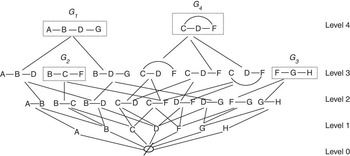
$$\[--><$> {\scr G} <$><!--$$, a lattice is a structural form used to model the search space for finding frequent subgraphs, where each vertex represents a connected subgraph of the graph in $$\[--><$> {\scr G} <$><!--$$ (Thomas et al., Reference Thomas, Valluri and Karlapalem2006). The lowest vertex depicts the empty subgraph and the vertexes at the highest level depict the graphs in $$\[--><$> {\scr G} <$><!--$$. A vertex p is a parent of the vertex q in the lattice, if q is a subgraph of p, and q is different from p by exactly one edge. The vertex q is a child of p. All the subgraphs of each graph $$\[--><$> {{G}_i}\, \in \,{\scr G} <$><!--$$ that occur in the database are present in the lattice, and every subgraph occurs only once in it.Example: given a graph data set
$$\[--><$> {\scr G}\, = \,{\rm{\{ }}{{G}_1},{{G}_2},{{G}_3},{{G}_4}{\rm{\} }} <$><!--$$, the corresponding $$\[--><$> Lattice{\rm{(}}{\scr G}{\rm{)}} <$><!--$$ is given in Figure 2. In the figure, the lowest vertex φ represents the empty subgraph, and the vertexes at the highest level correspond to G 1, G 2, G 3, and G 4. The parents of the subgraph B–D are subgraphs A–B–D (joining the edge A–B) and B–D–G (joining the edge D–G). Similarly, subgraphs B–C and C–F are the children of the subgraph B–C–F.Figure 2$$\[--><$>Lattice{\rm{(}}{\scr G}{\rm{)}}<$><!--$$(Figure based on a similar figure presented in Thomas et al., Reference Thomas, Valluri and Karlapalem2006)Free tree: An undirected graph that is connected and acyclic (Chi et al., Reference Chi, Nijssen, Muntz and Kok2004, Reference Chi, Yang, Xia and Muntz2004a).
Labelled unordered tree: A labelled unordered tree (an unordered tree, for short) is a directed acyclic graph (DAG) denoted as T(V, φ, E, vr), where V is a set of vertexes of T; φ is a labelling function, such that ∀vi ∈ V, φ(vi)→vi; E ⊆ V × V is a set of edges of T; and vr is a distinguished vertex called root of T. For ∀vi ∈ V, there is a unique path (vr, v 1, v 2, … ,vi) from the root vr to vi (Asai et al., Reference Asai, Abe, Kawasoe, Arimura, Satamoto and Arikawa2002, Reference Asai, Arimura, Uno and Nakano2003). If a vertex vi is on the path from the root to the vertex vj, then vi is an ancestor of vj, and vj is a descendant of vi. For each edge (vi, vj) ∈ E, vi is the parent of vj, and vj is a child of vi. Vertexes that share the same parent are siblings. The size of T is defined to be the number of vertexes in T. A vertex without any child is a leaf vertex; otherwise it is an intermediate vertex. The right-most path of T is the path from the root vertex to the right-most leaf. The depth (level) of a vertex is the length of the path Footnote 3 from the root to that vertex. The degree of a vertex v, denoted by degree (v), is the number of edges incident to it (West, Reference West2000; Chi et al., Reference Chi, Nijssen, Muntz and Kok2004, Reference Chi, Yang, Xia and Muntz2004a; Tan et al., Reference Tan, Dillon, Feng, Chang and Hadzic2005).
Labelled ordered tree: A labelled ordered treeFootnote 4 (an ordered tree, for short) is a labelled unordered tree but with a left-to-right ordering imposed among the children of each vertex (Asai et al., Reference Asai, Abe, Kawasoe, Arimura, Satamoto and Arikawa2002, Reference Asai, Arimura, Uno and Nakano2003; Chi et al., Reference Chi, Nijssen, Muntz and Kok2004).
Bottom-up subtree: Given a rooted tree T(V, φ, E, vr) (ordered or unordered),
$$\[--><$> \vec {T}{\rm{(}}\vec {V},\vec {\phi },\vec {E},{{\vec {v}}_r}{\rm{)}} <$><!--$$ is a bottom-up subtree of T, if and only if: (i) $$\[--><$> \vec {V}\, \subseteq \,V <$><!--$$, (ii) $$\[--><$> \vec {E}\, \subseteq \,E <$><!--$$, (iii) the labelling of $$\[--><$> \vec {V} <$><!--$$ and $$\[--><$> \vec {E} <$><!--$$ in T is preserved in $$\[--><$> \vec {T} <$><!--$$, (iv) ∀v ∈ V, if $$\[--><$> v\, \in \,\vec {V} <$><!--$$ then all descendants of v must also be in $$\[--><$> \vec {V} <$><!--$$, and (v) if T is ordered, then the left-to-right ordering among the siblings in T should be preserved in $$\[--><$> \vec {T} <$><!--$$ (Valiente, Reference Valiente2002; Chi et al., Reference Chi, Nijssen, Muntz and Kok2004).Induced subtree: Given a labelled tree T(V, φ, E, vr) (free tree or unordered tree or ordered tree),
$$\[--><$> \vec {T}{\rm{(}}\vec {V},\vec {\phi },\vec {E},{{\vec {v}}_r}{\rm{)}} <$><!--$$ is an induced subtree of T, if and only if: (i) $$\[--><$> \vec {V}\, \subseteq \,V <$><!--$$, (ii) $$\[--><$> \vec {E}\, \subseteq \,E <$><!--$$, (iii) the labelling of $$\[--><$> \vec {V} <$><!--$$ and $$\[--><$> \vec {E} <$><!--$$ in T is preserved in $$\[--><$> \vec {T} <$><!--$$, and ( iv) if defined for ordered trees, the left-to-right ordering among the siblings in $$\[--><$> \vec {T} <$><!--$$ should be a sub-ordering of the corresponding vertexes in T (Chi et al., Reference Chi, Nijssen, Muntz and Kok2004; Tan et al., Reference Tan, Dillon, Hadzic, Chang and Feng2006).Embedded subtree: Given a labelled tree T(V, φ, E, vr),
$$\[--><$> \vec {T}{\rm{(}}\vec {V},\vec {\phi },\vec {E},{{\vec {v}}_r}{\rm{)}} <$><!--$$ is an embedded subtree of T, if and only if: (i) $$\[--><$> \vec {V}\, \subseteq \,V <$><!--$$, (ii)$$\[--><$> \forall v\, \in \,\vec {V},\vec {\phi }{\rm{(}}v{\rm{)}}\, = \,\phi {\rm{(}}v{\rm{)}} <$><!--$$, (iii) $$\[--><$> \forall {\rm{(}}u,v{\rm{)}}\, \in \,\vec {E} <$><!--$$, such that u is the parent of v, u is an ancestor of v in T, and (iv) in the case of ordered trees, $$\[--><$> \forall {\rm{(}}u,v{\rm{)}}\, \in \,\vec {V},preorder{\rm{(}}u{\rm{)}}\, \less \,preorder{\rm{(}}v{\rm{)}} <$><!--$$ in $$\[--><$> \vec {T} <$><!--$$ if and only if preorder (u) < preorder (v) in T, where the pre-order of a vertex is its index in the tree, according to the pre-order traversalFootnote 5.



















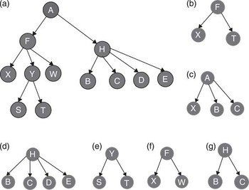
To summarize the above, Figure 3 gives some examples of bottom-up subtrees, induced subtrees, and embedded subtrees. In the figure: tree (a) on the left represents a data tree, trees (d) and (e) are two bottom-up subtrees of (a), trees (f) and (g) are two induced subtrees of (a), and trees (b) and (c) are two embedded subtrees of (a). The relationship among these three types of subtrees can be denoted as: bottom-up subtree ⊆ induce subtree ⊆ embedded subtree.
Different types of trees

2.2 Graph isomorphism detection
The kernel of FSM is (sub)graph isomorphism detection. Graph isomorphism is neither known to be solvable in polynomial time nor NP-complete, while subgraph isomorphism, where we wish to establish whether a subgraph is wholly contained within a supergraph, is known to be NP-complete (Garey & Johnson, Reference Garey and Johnson1979). When restricting the graphs to trees, (sub)graph isomorphism detection becomes (sub)tree isomorphism detection. Tree isomorphism detection can be solved in a linear time (see algorithm proposed in Hopcroft & Tarjan, Reference Hopcroft and Tarjan1972). Faster subtree isomorphism detection algorithms, with worst case time complexity of  $$\[--><$> {\scr O}{\rm{(}}{{k}^{{\rm{1}}{\rm{.5}}}} n{\rm{)}} <$><!--$$, were proposed by Matula (Reference Matula1978) and Chung (Reference Chung1987), and further improved upon by Shamir and Tsur (Reference Shamir and Tsur1999) in
 $$\[--><$> {\scr O}\left( {\frac{{{{k}^{{\rm{1}}{\rm{.5}}}} }}{{log\,k}}n} \right) <$><!--$$ time (k and n are the sizes of the subtree and the tree to be searched in terms of the number of vertexes).
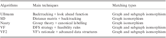
Subgraph isomorphism detection is fundamental to FSM. A significant number of ‘efficient’ techniques have been proposed, all directed at reducing, as far as possible, the computational overhead associated with subgraph isomorphism detection. Subgraph isomorphism detection techniques can be roughly categorized as being either: exact matching (Schmidt & Druffel, Reference Schmidt and Druffel1976; Ullmann, Reference Ullmann1976; McKay, Reference McKay1981; Cordella et al., Reference Cordella, Foggia, Sansone, Tortorella and Vento1998, Reference Cordella, Foggia, Sansone and Vento2001) or error tolerant matching (Shapiro & Haralick, Reference Shapiro and Haralick1981; Bunke & Allerman, Reference Bunke and Allerman1983; Christmas et al., Reference Christmas, Kittler and Petrou1995; Messmer & Bunke, Reference Messmer and Bunke1998). Most FSM algorithms adopt exact matching. A categorization of the main exact matching subgraph isomorphism detection algorithms is presented in Table 2. In Table 2, column two indicates the main methods employed to carry out the isomorphism detection, and column three indicates whether the isomorphism detection algorithm applies to graph isomorphism or subgraph isomorphism.
Categorization of exact matching (sub)graph isomorphism testing algorithms
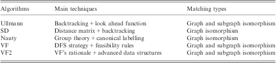
DFS = Depth First Search; SD = Schmidt and Druffel.
With reference to Table 2, Ullmann's algorithm employs a backtracking procedure with a look-ahead function to reduce the size of the search space (Ullmann, Reference Ullmann1976). The SD (Schmidt and Druffel) algorithm, in turn, utilizes a distance matrix representation of a graph with a backtracking procedure to reduce the search (Schmidt & Druffel, Reference Schmidt and Druffel1976). The Nauty algorithm (McKay, Reference McKay1981) uses group theory to transform graphs to be matched into a canonical form so as to provide for more efficient and effective graph isomorphism checking. However, it has been noted (Conte et al., Reference Conte, Foggia, Sansone and Vento2004) that the construction of the canonical forms can lead to exponential complexity in the worst case. Although Nauty was regarded as the fastest graph isomorphism algorithm by Conte et al. (Reference Conte, Foggia, Sansone and Vento2004), Miyazaki (Reference Miyazaki1997) demonstrated that there exists some categories of graphs, which required exponential time to generate the canonical labelling. The VF (Cordella et al., Reference Cordella, Foggia, Sansone, Tortorella and Vento1998) and VF2 (Cordella et al., Reference Cordella, Foggia, Sansone and Vento2001) algorithms use a Depth First Search (DFS) strategy, assisted by a set of feasibility rules to prune the search tree. VF2 is an improved version of VF that explores the search space more effectively so that the matching time and the memory consumption are significantly reduced. In Foggia et al. (Reference Foggia, Genna and Vento2001), a detailed experimental analysis of these five algorithms is provided to indicate that none of the existing algorithms is completely superior to the others. In general, VF2 was found to give the best performance with respect to the size and the type of graphs to be matched.
3 Overview of frequent subgraph mining
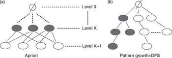
This section provides a generic overview of the process of FSM. It is widely accepted that FSM techniques can be divided into two categories: (i) Apriori-based approaches and (ii) pattern growth-based approaches. These two categories are similar in spirit to counterparts found in ARM, namely the Apriori algorithm (Agrawal & Srikant, Reference Agrawal and Srikant1994) and Frequent Pattern (FP)-growth algorithm (Han et al., Reference Han, Pei and Yin2000), respectively. The Apriori-based approach proceeds in a generate-and-test manner using a Breadth First Search (BFS) strategy to explore the subgraph lattice of the given database. Therefore, before considering (k + 1) subgraphs, this approach has to first consider all k subgraphs. The pattern growth-based adopts a DFS strategy is depicted where, for each discovered subgraph g, the subgraph is extended recursively until all frequent supergraphs of g are discovered (Han & Kamber, Reference Han and Kamber2006). The distinction between the two approaches is illustrated in Figure 4.
Two types of search space. Note that the subgraph lattice is shown ‘upside-down’. Vertexes corresponding to graphs with fewer edges are displayed at the top of the picture in each case

Apriori-based approach

The basic Apriori-based algorithm is presented in 3.1. In line 5, all frequent (k − 1) subgraphs are used to generate k subgraph candidates. If any of the k − 1 candidate subgraphs are not frequent, then the DCP (see Section 2) can be used to safely prune the candidates. Most existing FSM approaches adopt an iterative pattern mining strategy, where each iteration can be divided into two phases: (i) candidate generation (line 5 in Algorithm 3.1) and (ii) support computation (lines 6–12 in Algorithm 3.1). Generally, research on FSM focuses on these two phases using a variety of techniques. Since it is harder to address subgraph isomorphism detection, more research effort is directed at how to efficiently generate subgraph candidates. Because subtree isomorphism detection can be solved in  $$\[--><$> {\scr O}\left( {\frac{{{{k}^{{\rm{1}}{\rm{.5}}}} }}{{log\,k}}n} \right) <$><!--$$ time, the computational complexity is reduced within the context of FSM. Therefore, the survey presented in this paper makes a distinction between FSM and frequent subtree mining. In the rest of this paper, we will continue to use the acronym FSM to mean both frequent subgraph and subtree mining; and the acronyms FGM and FTM to indicate frequent subgraph and subtree mining, respectively, where a distinction is required.
Before considering specific subgraph and subtree mining algorithms in detail (Sections 4 and 5), techniques used to represent graphs and trees will first be considered. The aim here is to represent graphs and trees in such a manner that subgraphs can be enumerated efficiently so as to facilitate the desired FSM.
3.1 Canonical representations
The simplest mechanism whereby a graph structure can be represented is by employing an adjacency matrix or adjacency list. Using an adjacency matrix, the rows and columns represent vertexes, and the intersection of row i and column j represents a potential edge, connecting the vertexes vi and vj. The value held at intersection <i, j> typically indicates the number of links from vi to vj. However, the use of adjacency matrices, although straightforward, does not lend itself to isomorphism detection, because a graph can be represented in many different ways depending on how the vertexes (and edges) are enumerated (Washo & Motoda, Reference Washo and Motoda2003). With respect to isomorphism testing, it is therefore desirable to adopt a consistent labelling strategy that ensures that any two identical graphs are labelled in the same way regardless of the order in which vertexes and edges are presented (i.e. a canonical labelling strategy).
A canonical labelling strategy defines a unique code for a given graph (Read & Corneil, Reference Read and Corneil1977; Fortin, Reference Fortin1996). Canonical labelling facilitates isomorphism checking because it ensures that if a pair of graphs are isomorphic, then their canonical labellings will be identical (Kuramochi & Karypis, Reference Kuramochi and Karypis2001). One simple way of generating a canonical labelling is to flatten the associated adjacency matrix by concatenating rows or columns to produce a code comprising a list of integers with a minimum (or maximum) lexicographical ordering imposed. To further reduce the computation resulting from the permutations of the matrix, canonical labellings are usually compressed, using what is known as a vertex invariant scheme (Read & Corneil, Reference Read and Corneil1977), that allows the content of an adjacency matrix to be partitioned according to the vertex labels. Various canonical labelling schemes have been proposed, some of the more significant are described in this subsection.
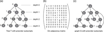
Minimum depth first search code (M-DFSC): There are a number of variants of DFS encodings, but essentially each vertex is given a unique identifier (ID) generated from a DFS traversal of a graph (DFS subscripting). Each constituent edge of the graph in the DFS code is then represented by a 5-tuple: (i, j, li, le, lj), where i and i are the vertex IDs, li and lj are the labels for the corresponding vertexes, and le is the label for the edge connecting the vertexes. On the basis of the DFS lexicographic order, the M-DFSC of a graph g can be defined as the canonical labelling of g (Yan & Han, Reference Yan and Han2002). The DFS codes for the left-most branch and the right-most branch of the example graph in Figure 5c are {(0, 1, a, 1, b), (1, 2, b, 1, e), (2, 3, e, 1, f), (3, 4, f, 1, c), (4, 2, c, 1, e)} and {(0, 9, a, 1, d), (9, 10, d, 1, f), (10, 11, f, 1, g), (11, 9, g, 1, d)}, respectively.
Figure 5Graph examples to illustrate the canonical representations discussed in Subsection 3.1 (for ease of illustration, all edge labels are assumed to be the same and represented by ‘1’)
Canonical adjacency matrix (CAM): Given an adjacency matrix M of a graph g, an encoding of M can be obtained by the sequence obtained from concatenating the lower (or upper) triangular entries of M, including entries on the diagonal. Since different permutations of the set of vertexes correspond to different adjacency matrices, the canonical (CAM) form of g is defined as the maximal (or minimal) encoding. The adjacency matrix from which the canonical form is generated defines the Canonical Adjacency Matrix or CAM (Inokuchi et al., Reference Inokuchi, Washio and Motoda2000, Reference Inokuchi, Washio, Nishimura and Motoda2002; Kuramochi & Karypis, Reference Kuramochi and Karypis2001; Huan et al., Reference Huan, Wang and Prins2003). The encoding for the example graph given in Figure 5c, represented by the matrix in Figure 5b, is thus {a1b00c100d0110e00111f000101g1000010h00000001k000001000w}.

The above two schemes are applicable to any simple undirected graph. However, it is easier to define a canonical labelling for trees than graphs, because trees have an inherent structure associated with them. There also exist more specific schemes that are uniquely focused on trees. Among these, DFS-LS and DLS are directed at rooted ordered trees, BFCS and DFCS are used for rooted unordered trees. Each of these will be briefly described below.
DFS label sequence (DFS-LS): Given a labelled ordered tree T, the labels of ∀vi ∈ V are added to a string S, during a DFS traversal of T. Whenever backtracking occurs, a unique symbol, such as ‘−1’ or ‘$’ or ‘/’, is added to S (Zaki, Reference Zaki2002, Reference Zaki2005a; Tan et al., Reference Tan, Dillon, Hadzic, Chang and Feng2006). The DFS-LS code for the example tree given in Figure 5a is thus {abea$$$cfb$d$$a$$dfc$$$}.
Depth-label sequence (DLS): Given a labelled ordered tree T, depth-label pairs comprising the depth and label ∀vi ∈ V, (d(vi), l(vi)), are added to a string S during a DFS traversal of T. The DLS of T is defined as S = {(d(v 1), l(v 1)), …, (d(vk), l(vk))} (Asai et al., Reference Asai, Abe, Kawasoe, Arimura, Satamoto and Arikawa2002; Wang et al., Reference Wang, Hong, Pei, Zhou, Wang and Shi2004a). The DLS code for the example tree given in Figure 5a is {(0,a), (1,b), (2,e), (3,a), (1,c), (2,f), (3,b), (3,d), (2,a), (1,d), (2,f), (3,c)}.
Breadth-first canonical string (BFCS): For a labelled ordered tree, every vertex label is added to a string S, by traversing the tree in a BFS manner. In addition, a ‘$’ symbol is used to partition the families of siblings, and a ‘#’ symbol is used to indicate the end of the string encoding. ‘$’ is considered to be lexicographically before ‘#’ and both of them order greater than any other vertex and edge labels. Given an unordered tree T, different ordered trees with corresponding BFS string encodings can be produced by imposing different orderings on the children of the intermediate vertexes. The BFCS of T is the lexicographically minimal of these encodings, and the corresponding rooted ordered tree defines the breadth-first canonical form (BFCF) of T (Chi et al., Reference Chi, Yang, Xia and Muntz2005). BFCS's variants can be found in Chi et al. (Reference Chi, Yang, Xia and Muntz2003, Reference Chi, Yang, Xia and Muntz2004a). Thus, the BFS string encoding of the example tree given in Figure 5a is a$bcd$e$fa$f$a$bd$$c#.
Depth-first canonical string (DFCS): Similar to the BFCS but using DFS, the depth-first string encoding, for a labelled ordered tree, labels each vertex by traversing the tree in a DFS manner. The DFCS of a unordered tree T is then the minimal of all the possible DFS encodings, according to the lexicographical ordering. The corresponding rooted ordered tree defines the depth-first canonical form (DFCF) of T (Chi et al., Reference Chi, Yang, Xia and Muntz2005). DFCS's variants can also be found in Chi et al. (Reference Chi, Yang, Xia and Muntz2003, Reference Chi, Yang, Xia and Muntz2004b). The DFS string encoding of the example tree given in Figure 5a is abea$$$$cfb$d$$a$$dfc$$$#.
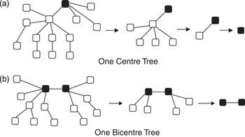
Canonical representation of free trees: Free trees do not have roots. In this case, a unique representation for a free tree is usually constructed by selecting one vertex or a pair of vertexes as the root(s). The procedure starts with removing all leaf vertexes and their incident edges recursively until a single vertex or two adjacent vertexes are left. In the first case, the remaining vertex is called the centre, and a rooted unordered tree is obtained with the centre as the root. The procedure is displayed in Figure 6a. In the second case, the pair of remaining vertexes are called the bi-centre; a pair of rooted unordered trees are obtained with the bi-centre as the roots (along with an edge connecting the two roots). The procedure is illustrated in Figure 6b. Thus, a pair of trees is ordered so that the root of the smaller one is chosen as the root of the whole tree (Chi et al., Reference Chi, Yang, Xia and Muntz2003; Rückert & Kramer, Reference Rückert and Kramer2004). After obtaining rooted unordered trees, any canonical representations for rooted unordered trees (see above) can be employed to represent the free trees.
Figure 6An example of two types of free trees

3.2 Candidate generation
As noted earlier, candidate generation is an essential phase in FSM. How to systematically generate candidate subgraphs without redundancy (i.e. each subgraph should be generated only once) is a key issue. Many FSM algorithms can be characterized by the strategy adopted for candidate generation. A number of the most significant are briefly described below. Since a significant proportion of strategies employed in FTM is interwoven with those employed in FGM, no clear distinction can be made between candidate generation strategies in terms of FTM and FGM, that is, strategies initially proposed for (say) FGM are equally applicable to FTM and vice versa.
3.2.1 Level-wise join
The level-wise join strategy was introduced by Kuramochi and Karypis (Reference Kuramochi and Karypis2001). Basically, a (k + 1) subgraphFootnote 6 candidate is generated by combining two frequent k subgraphs that share the same (k − 1) subgraph. This common (k − 1) subgraph is referred to as a core for these two frequent k subgraphs. The main issue concerning this strategy is that one k subgraph can have at most k different (k − 1) subgraphs and the joining operation may generate many redundant candidates. In Kuramochi and Karypis (Reference Kuramochi and Karypis2004a), this issue was addressed by limiting the (k − 1) subgraphs to the two (k − 1) subgraphs with the smallest and the second smallest canonical labels. By carrying out this adapted join operation, the number of duplicate candidates generated was significantly reduced. Other algorithms that adopted this strategy, and its variants, are AGM (Inokuchi et al., Reference Inokuchi, Washio and Motoda2000), DPMine (Vanetik et al., Reference Vanetik, Gudes and Shimony2002; Gudes et al., Reference Gudes, Shimony and Vanetik2006), and HSIGRAM (Kuramochi & Karypis, Reference Kuramochi and Karypis2005), which will be discussed later.
3.2.2 Right-most path expansion
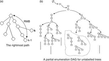
Right-most path expansion is the most common candidate generation strategy, which generates (k + 1)-subtrees from frequent k-subtrees by adding vertexes only to the right-most path of the tree (Asai et al., Reference Asai, Abe, Kawasoe, Arimura, Satamoto and Arikawa2002, Reference Asai, Arimura, Uno and Nakano2003; Zaki, Reference Zaki2002; Nijssen & Kok, Reference Nijssen and Kok2003). In Figure 7a, ‘RMB’ denotes the right-most branch, which is the path from the root to the right-most leaf (k − 1), and a new vertex k is added by attaching it to any vertexes along the RMB. An enumeration DAG using right-most expansion is a tree with a root φ, where each node is a subtree pattern. A node S is linked by another node T if and only if T is a right-most expansion of S. Every 1-subtree is a right-most expansion of the root φ and every (k + 1)-subtree is a right-most expansion of the k-subtree. Hence, all subtree patterns can be enumerated by traversing in either BFS or DFS manner (Asai et al., Reference Asai, Abe, Kawasoe, Arimura, Satamoto and Arikawa2002). Figure 7b shows a part of an enumeration DAG grown by right-most path expansion. Each square in the figure represents a vertex in the tree. An enumeration DAG (sometimes also simplified as an enumeration tree) is used to illustrate how a set of patterns is completely enumerated in a search problem. Enumeration DAGs have been used extensively in ARM (Bayardo, Reference Bayardo1998; Agrawal et al., Reference Agrawal, Aggarwal and Prasad2001); and subsequently, in a variety of ways, by many subtree mining algorithms (Asai et al., Reference Asai, Abe, Kawasoe, Arimura, Satamoto and Arikawa2002, Reference Asai, Arimura, Uno and Nakano2003; Nijssen & Kok, Reference Nijssen and Kok2003; Chi et al., Reference Chi, Yang, Xia and Muntz2004a, Reference Chi, Yang, Xia and Muntz2005).
An illustration of right-most path expansion

3.2.3 Extension and join
The extension and join strategy was first proposed by Huan et al. (Reference Huan, Wang and Prins2003), and later used by Chi et al. (Reference Chi, Yang, Xia and Muntz2004a). It employed a BFCS representation, whereby a leaf at the bottom level of a BFCF tree is defined as a ‘leg’. For a node ‘Vn’ in an enumeration tree, if the height of the BFCF tree corresponding to ‘Vn’ is assumed to be h, all children of ‘Vn’ can be obtained by either of the following two operations:
(a) Extension operation: Adding a new leg at the bottom level of the BFCF tree yields a new BFCF with height h + 1.
(b) Join operation: joining ‘Vn’ and one of its sibling yields a new BFCF with height h.
3.2.4 Equivalence class-based extension
Equivalence class-based extension (Zaki, Reference Zaki2002, Reference Zaki2005b) is founded on a DFS-LS representation for trees. Basically, a (k + 1)-subtree is generated by joining two frequent k-subtrees. The two k-subtrees must be in the same equivalence class [C]Footnote 7. An equivalence class consists of the class prefix encoding and a list of members. Each member of the class can be represented as a (l, p) pair, where l is the k-th vertex label and p is the depth-first position of the k-th vertex's parent. It is verified, in Zaki (Reference Zaki2002), that all potential (k + 1)-subtrees with the prefix [C] of size (k − 1) can be generated by joining each pair of members of the same equivalent class [C].
3.2.5 Right-and-left tree join
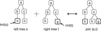
The right-and-left tree join strategy was proposed by Hido and Kawano (Reference Hido and Kawano2005). It essentially uses the right-most leaf (see 2) and left-most leafFootnote 8 of the tree to generate candidates in a BFS manner. Let lml(T) denote the left-most leaf of T and Right(T) the right-most tree obtained by removing lml(T); and let rml(T) denote the right-most leaf and left(T) the left tree obtained by removing rml(T). Given two trees s and t, where Right(s) = Left(t), their right-and-left tree join is defined as: join(s, t) = s ∪ rml(t) = lml(s) ∪ t A diagram depicting this join operation is given in Figure 8.
An illustration of right-and-left tree join

Among these candidate generation strategies, the level-wise join and the extension and join are directed at FGM, and all others at FTM.
4 Frequent subtree mining algorithms
The previous section considered the joint issues of representation (canonical forms) and candidate generation, in terms of both trees and graphs. In this section, a number of prominent FTM algorithms are reviewed. FTM has attracted a great deal of research interest in areas such as: network IP multicastFootnote 9 routing (Cui et al., Reference Cui, Kim, Maggiorini, Boussetta and Gerla2005), web usage mining (Zaki, Reference Zaki2005b), computer vision (Liu & Geiger, Reference Liu and Geiger1999), XML mining (Zaki & Aggarwal, Reference Zaki and Aggarwal2003; Tan et al., Reference Tan, Dillon, Feng, Chang and Hadzic2005), bio-informatics (Hein et al., Reference Hein, Jiang, Wang and Zhang1996; Rückert & Kramer, Reference Rückert and Kramer2004; Zhang & Wang, Reference Zhang and Wang2006), and so on. The attraction of frequent subtree mining is that subgraph isomorphism detection becomes subtree isomorphism detection, which can be solved in  $$\[--><$> {\scr O}\left( {\frac{{{{k}^{{\rm{1}}{\rm{.5}}}} }}{{log\,k}}n} \right) <$><!--$$ time (Shamir & Tsur, Reference Shamir and Tsur1999). In addition, the structure of trees may be usefully employed to simplify the overall mining process.
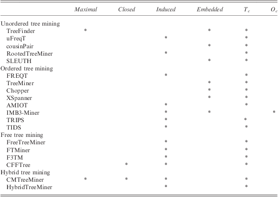
The FTM algorithms discussed in this section have been categorized as in Table 3, according to the nature of the trees that the FTM algorithm is directed at: (i) unordered trees, (ii) ordered trees, (iii) free trees, or (iv) hybrid trees (any combinations of (i), (ii), and (iii)). The algorithms are also categorizations according to the nature of the subtrees to be output (maximal subtrees, closed subtrees, induced subtrees, or embedded subtrees), and the nature of the support metrics employed (transaction-based counting, denoted by Tc; or occurrence-based counting, denoted by Oc). For an alternative review of FTM algorithms, readers may like to refer to Chi et al. (Reference Chi, Nijssen, Muntz and Kok2004), who provide a theoretical foundation and performance study of a representative collection of FTM algorithms proposed prior to 2004.
Categorization of common frequent subtree mining algorithms

4.1 Unordered tree mining
Labelled unordered trees are often used to model structural data, two popular areas of application are the analysis of chemical compounds and the hyper-link structure of the web (Asai et al., Reference Asai, Arimura, Uno and Nakano2003).
Unordered tree FTM tends to use DLS-LS, DLS, or BFCS to represent the trees (as described in Subsection 3.1). An often cited, example of a DLS-DS-based algorithm is the SLEUTH Algorithm (Zaki, Reference Zaki2005a). SLEUTH is founded on earlier work directed at the FTM of other types of trees. This algorithm uses scope-lists to compute the support. Zaki et al. (2005a) considered two extension mechanisms for candidate generation: (i) class-based extension and (ii) canonical extension. Using class-based extension, not all candidates generated by this mechanism necessarily adhere to the desired canonical form, consequently it is necessary to check each candidate subtree to ensure that it is in canonical form. Alternatively, canonical extension can be applied only to canonical frequent subtrees that have a known frequent edge; however, this results in many infrequent but canonical candidates. As noted by Zaki (Reference Zaki2005a), there is a trade-off between using the two extension mechanisms. Experiments conducted by Zaki (Reference Zaki2005a) demonstrated that using class-based extension is more efficient than canonical extension.
An established example of an unordered tree FTM algorithm that uses the DLS representation is uFreqT (Nijssen & Kok, Reference Nijssen and Kok2003). At the candidate generate phase, uFreqT uses the right-most path expansion technique to generate candidates. At the support counting phase, a tree mapping algorithm, to determine the frequency of the current pattern, is translated into a more computationally efficient maximum bipartite-matching algorithm. In order to facilitate this support counting, uFreqT maintains a data structure in which to store all potential mappings for the vertexes on the right-most path and pointers to the parent mappings.
Chi et al. (Reference Chi, Yang, Xia and Muntz2005) presented an algorithm, RootedTreeMiner, founded on a BFCS encoding. Unlike SLEUTH or uFreqT, RootedTreeMiner is directed at finding only frequent induced subtrees. Thus, at the candidate generation phase, the range of allowable vertexes at a given position can be computed beforehand. At the support counting phase, an occurrence list is first built for each discovered subtree t. This list records the ID of each graph transaction in the tree data set that contains t, along with the mapping between the vertex indexes in t and those in the transaction. Using this occurrence list, the support of t equates to the number of elements in the list that have distinct IDs.
The above all employ exact matching techniques. An example of an unordered tree FTM that employs inexact matching is TreeFinder (Termier et al., Reference Termier, Rousset and Sebag2002). Treefinder employs an Apriori-based approach, using an ancestor–descendant relationship, to mine embedded subtrees. Algorithms that employ inexact matching are, of course, not guaranteed to discover the complete set of frequent subtrees; however, they tend to be very efficient.
Some unordered tree FTM algorithms are directed at specific applications and can use features of these applications to enhance the efficiency of the operation of the algorithm. For example, Shasha et al. (Reference Shasha, Wang and Zhang2004) presented an unordered tree FTM algorithm, cousinPair, for application to phylogeny. They defined an interesting pattern as being a ‘cousin pair’, a pair of vertexes satisfying some cousin distance and minimum occurrence threshold. By using such constraints, interesting patterns were mined from a tree database. The objective here was to get a better understanding of the evolutionary history of species. The obvious disadvantage of algorithms such as cousinPair is that they are not generally applicable.
4.2 Ordered tree mining
In contrast to unordered tree mining, the ordering inherent in ordered trees can be used to introduce efficiencies with respect to subtree generation and subtree isomorphism testing. Candidate subtrees are typically grown using right-most path extension or equivalence class-based extension. For example, Asai et al. (Reference Asai, Abe, Kawasoe, Arimura, Satamoto and Arikawa2002) used right-most expansion with respect to their FREQT algorithm. In addition, only the right-most leaf occurrences of the patterns are saved so as to make the support counting more efficient. Asai et al. modelled semi-structured data (namely Web pages), using a labelled ordered tree to evaluate FREQT.
The advantage of right-most expansion with respect to ordered trees is that the generation of duplicate candidate sets can be avoided. Hido and Kawano (Reference Hido and Kawano2005) noted that enumeration using right-most path expansion, as adopted by FREQT and other FSM algorithms, tends to generate many non-frequent candidates, thus resulting in unnecessary support counting. Consequently, Hido and Kawano introduced an algorithm, AMIOT, to utilize a new enumeration scheme to reduce the number of non-frequent candidates while maintaining the advantage offered by right-most expansion. This scheme, right-and-left tree join, guaranteed that the set of subtree candidates was always a subset of that achieved by the enumeration using right-most path expansion. The performance of AMIOT, with respect to both synthetic data and XML data, demonstrated that it was scalable and performed faster than FREQT. However, the memory usage of AMIOT is larger than that of FREQT, due to the nature of the BFS strategy used by AMIOT.
Zaki (Reference Zaki2002) proposed a FTM algorithm, TreeMiner, that uses equivalence class-based extension (coupled with a DFS-LS representation). The notion of scope-lists, later also employed in SLEUTH (see above) was also developed to facilitate fast support counting. Unlike FREQT and AMIOT, TreeMiner is directed at discovering frequent embedded subtrees. The performance of the algorithm was compared with a base algorithm, PatternMatcher, which employed a BFS strategy. The experimental results demonstrated that TreeMiner outperformed PatternMatcher when applied to real data. However, the pruning technique adopted by TreeMiner is not as efficient as that used by PatternMatcher, given a low support threshold. TreeMiner is a frequently referenced FTM algorithm.
Wang et al. (Reference Wang, Hong, Pei, Zhou, Wang and Shi2004a) also proposed an algorithm, Chopper, to mine frequent embedded subtrees from tree data sets, but used a DLS representation. Chopper first uses a revised PrefixSpan (Pei et al., Reference Pei, Han, Mortazavi-Asl, Pinto, Chen, Dayal and Hsu2001) to mine frequent sequential patterns. Then the tree database is again scanned, with reference to the discovered sequential patterns, to generate candidate patterns and support counts. The two processes of sequential pattern mining and subtree pattern verification are separated in Chopper, and thus an additional computational overhead is incurred. In order to improve the efficiency of Chopper, the XSpanner algorithm was subsequently produced to integrate the sequential pattern mining into the process of subtree pattern verification. Using projected database techniques, XSpanner grew larger frequent subtrees from smaller ones starting from one vertex. Both Chopper and XSpanner outperform TreeMiner when the support threshold is below 5%. However, XSpanner was found to be more stable than Chopper when the support threshold was further reduced.
IMB3-Miner (Tan et al., Reference Tan, Dillon, Hadzic, Chang and Feng2006) is also directed at frequent embedded subtree mining (from ordered tree data sets), but uses a parameter with which to control the level of embedding Footnote 10. When the level of embedding is equal to 1, the discovered frequent subtrees are induced subtrees. Thus, by adjusting the embedding level, the algorithm can be used to mine both induced and embedded subtrees. By combining an Embedding List data structure with the TMG enumeration strategy (a specialized right-most path expansion strategy), IMB3-Miner guarantees that candidate subtrees are generated without duplication. Furthermore, an occurrence list is stored for each generated subtree to speed-up support counting. Unlike the foregoing, instead of using Tc, O c is employed to calculate the support of patterns. It has been experimentally demonstrated that IMB3-Miner achieves higher performance and scalability than TreeMiner and FREQT. The usage of Oc, instead of Tc, is typically adopted where the repetition and order of the patterns are important.
Tatikonda et al. (Reference Tatikonda, Parthasarathy and Kurc2006) proposed the TRIPS and TIDS algorithms to mining induced or embedded subtrees in a database of rooted ordered trees. TRIPS uses prüfer sequencingFootnote 11 and the left-most pathFootnote 12 of the pattern as the extension position. TIDS uses DFS sequencing and right-most path extension. The support computation for both algorithms employs an embedding list, an array-based structure, to facilitate the recursive generation of the patterns. There is a trade-off between the cost of maintaining the embedding lists and the efficiency of the support computation, when the number of distinct vertex labels is low compared with the total number of vertexes in the data set. Experiments demonstrated that both TRIPS and TIDS performed better than TreeMiner in terms of execution time and memory usage on both synthetic and real data sets. Both TRIPS and TIDS were found to be scalable when the database size increased and able to mine large databases even when using low support threshold values.
4.3 Free tree mining
Free tree mining algorithms, as the name suggests, are directed at the discovery frequent subtrees in collections of free trees. An early example is FreeTreeMiner (Chi et al., Reference Chi, Yang, Xia and Muntz2003) where a self-join operation was used for candidate subtree generation and a subtree isomorphism algorithm or support computation (Chung, Reference Chung1987). Experiments demonstrated that FreeTreeMiner can handle large real data well with a large range of support values; however, it was not found to be scalable when the size of the maximal frequent subtrees was increased, due to the exponential growth of the subtrees.
Similar work conducted by Rückert and Kramer (Reference Rückert and Kramer2004) defined a canonical representation for labelled free trees. This was embedded in a free tree mining algorithm, FTMiner. The algorithm extended more than one vertex at each recursive step during the candidate generation phase. It also adopted the concept of an extension table, which is a data structure for storing all the extensions for a subtree pattern along with the set of graph transactions containing the pattern. Utilizing this extension table, the algorithm not only kept track of the frequency of each subtree pattern, but also gathered information required for the extension of the current pattern, thus reducing significantly the number of database scans. Experiments on a large scale database suggest that the algorithm is able to mine frequent patterns among a collection of more than 37 330 chemical compounds using support threshold of 2%.
With the focus mainly on reducing the cost of candidate generation, Zhao and Yu (Reference Zhao and Yu2006) presented the F3TM free tree mining algorithm. The algorithm introduced the idea of an extension frontier to define the positions (vertexes) for growing frequent subtrees in the candidate generation phase, and uses automorphism-based pruning and canonical pruning techniques to enhance the efficiency of candidate generation. Compared with other free tree mining algorithms, performance studies indicated that F3TM was more efficient than FTMiner and FreeTreeMiner with respect to a chemical database of 42 390 compounds. CFFTree (Zhao & Yu, Reference Zhao and Yu2007) is an extension of F3TM directed at closed FTM. CFFTree employs a mechanism called safe position pruning to grow subtrees only on safe positions, thus introducing efficiencies when deciding which branch of the enumeration tree to prune. In addition, CFFTree employs safe label pruning to grow subtrees only on the vertexes with labels lexicographically less than the new ‘adding vertex’; this then serves to remove some unnecessary enumeration. The reported evaluation of CFFTree demonstrated that it outperformed its base algorithm, F3TM, using post-processing when finding closed patterns.
4.4 Hybrid tree mining
Hybrid tree mining algorithms are directed at more generic tree formats. As such they can be categorized as being directed at either: (i) unordered or free trees or (ii) ordered or unordered trees. An example of the first is HybridTreeMiner and an example of the second is CMTreeMiner.
HybridTreeMiner (Chi et al., Reference Chi, Yang, Xia and Muntz2004a) uses a BFCS representation. In the enumeration tree, each node represents an unordered tree in BFCF. For a node v in the enumeration tree, all the children of v may be generated using either an extension or a join operation. The join operation is applied to pairs of sibling nodes with a height (depth) of h, resulting in a BFCF tree with the same height. The extension operation is applied by extending a new leaf at the bottom level of the BFCF tree with a height of h, resulting in a BFCF tree with a height of (h + 1). This hybrid enumeration strategy was further extended to handle the free tree case. Reported experimental results demonstrated that HybridTreeMIner was faster than FreeTreeMiner, and that its memory usage was also much less than that required by FreeTreeMiner.
CMTreeMiner was introduced to mine both closed and maximal frequent subtrees in collections of labelled ordered or unordered trees (Chi et al., Reference Chi, Yang, Xia and Muntz2004b). By using pruning and heuristic techniques, the enumeration tree was grown only on the branches that can potentially produce closed or maximal frequent subtrees, thus avoiding the computational overhead associated with finding all frequent subtrees. The advantage offered by CMTreeMiner is that it directly mines closed and maximal frequent subtrees without first generating all frequent subtrees. Experimental results showed that: (i) for an ordered tree, database CMTreeMiner outperformed FREQT and (ii) for an unordered tree, database CMTreeMiner ran faster than HybridTreeMiner.
4.5 Summary of frequent subtree mining algorithms
From the foregoing it can be seen that many different methods, techniques, and strategies have been proposed to achieve FTM. From the perspective of applications, these algorithms can be divided into three main domains:
(a) Web access analysis: Examples are SLEUTH, RootedTreeMiner, TreeMiner, IMB3-Miner, Chopper, XSpanner, TRIPS, TIDS, CMTreeMiner, and HybridTreeMiner.
(b) IP multicast analysis: Examples are FreeTreeMiner and CMTreeMiner.
(c) Chemical compound analysis: Examples are FreeTreeMiner, FTMiner, F3TM, CFFTree, and HybridTreeMiner.
From the perspective of the traversing strategy employed in the search space, FTM algorithms can be categorized into two groups:
(a) BFS strategy: The BFS strategy has the advantage of performing full pruning, which, however, requires significant memory usage. Examples are RootedTreeMiner, AMIOT, FreeTreeMiner, and HybridTreeMiner.
(b) DFS strategy: The DFS strategy has the disadvantage of weak pruning. However, the memory usage is smaller than that required for BFS. Examples are uFreqT, SLEUTH, FREQT, TreeMiner, IMB3-Miner, TIDS, FTMiner, and CMTreeMiner.
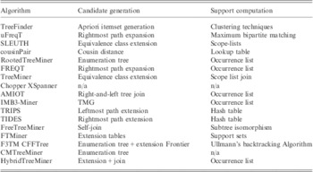
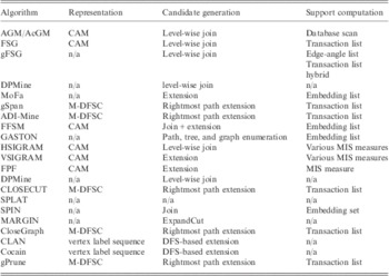
Table 4 lists the main techniques used for candidate generation and support counting with respect to the algorithms described in this section. Generally, each frequent subtree mining algorithm has its strengths and weaknesses. There is no universally applicable frequent subtree mining algorithm. In terms of FTM efficiency, the following techniques are considered to offer the best performance:
Summary of popular FTM algorithms and their candidate generation and support computation mechanisms

FTM = Frequent subtree mining; TMG = Tree Model Guided.
• DFS sequence and its variants for tree representation.
• DFS strategy for traversing the search space.
• Enumeration tree growth with right-most path expansion in candidate generation phase.
• Occurrence list for support counting.
Examples of algorithms containing at least three of these techniques are SLEUTH, FREQT, TreeMiner, and IMB3-Miner. Among these, FREQT and TreeMiner are usually chosen as base algorithms for comparison with others. TreeMiner is an Apriori-like FTM algorithm, while FREQT is a right-most path expansion style algorithm. These two styles represent two streams within the realm of FTM. Although subtree isomorphism can be solved in  $$\[--><$> {\scr O}\left( {\frac{{{{k}^{{\rm{1}}{\rm{.5}}}} }}{{log\,k}}n} \right) <$><!--$$ time, very few frequent subtree mining algorithms adopted it directly for support counting; occurrence lists are more frequently adopted. The main reason for this is that occurrence list counting is much more straightforward to implement.
5 Frequent subgraph mining algorithms
As was indicated in Figure 1b, FGM algorithms find substantial application in chemical informatics and biological network analysis. There are a variety of FGM algorithms reported in the literature. As in the case of FTM, candidate generation and support counting are key issues. Since subgraph isomorphism detection is known to be NP-complete, a significant amount of research work has been directed at various approaches for effective candidate generation. The mechanism employed for candidate generate is the most significant distinguishing feature of such algorithms. An exploration of current well-known FSM algorithms is provided in this section. Interested readers should note that a good review of the theoretical foundation of FGM, prior to 2003, can be found in Washo and Motoda (Reference Washo and Motoda2003). A more recent review of mining frequent patterns, including itemsets, subsequence, and subgraphs, appears in Han et al. (Reference Han, Cheng, Xin and Yan2007).
For discussion purposes, the FGM algorithms examined in this section are categorized into ‘general purpose’ and ‘pattern dependent’ FGM. The distinction is that in the latter case the nature of the patterns to be discovered is in some way specialized or limited because of the nature of the application domain (e.g. we are only interested in subgraphs satisfying some specific constraints). Consequently, knowledge of the nature of these special patterns allows for a reduction of the search space.
5.1 General purpose frequent subgraph mining
In this subsection a number of general purpose FGM algorithms are considered. To aid the discussion the algorithms are categorized according to three criteria: (i) the completeness of the search (exact search or inexact search), (ii) the type of input (transactions graphs or one single graph), and (iii) the search strategy (BFS or DFS).
5.1.1 Inexact frequent subgraphs mining
Inexact search-based FGM algorithms use an approximate measure to compare the similarity of two graphs, that is, any two subgraphs are not required to be entirely identical to contribute to the support count, instead a subgraph may contribute to the support count for a candidate subgraph if it is in some sense similar to the candidate. Inexact search is of course not guaranteed to find all frequent subgraphs, but the nature of the approximate graph comparison often leads to computational efficiency gains. There are only a few examples of inexact FSM algorithms in the literature. However, one frequently quoted example is the SUBDUE algorithm (Cook & Holder, Reference Cook and Holder1994, Reference Cook and Holder2000). SUBDUE uses the minimum description length principle to compress the graph data; and a heuristic beam search method, that makes use of background knowledge, to narrow down the search space. Although the application of SUBDUE shows some promising results in domains such as image analysis and CAD circuit analysis, the scalability of the algorithm is an issue, that is, the run time does not increase linearly with the size of the input graph. Furthermore, SUBDUE tends to discover only a small number of patterns.
Another inexact search-based FGM algorithm is GREW (Kuramochi & Karypis, Reference Kuramochi and Karypis2004b). However, GREW is directed at finding connected subgraphs, which have many vertex-disjoint embeddingsFootnote 13 in single large graphs. GREW uses a heuristic-based approach that is claimed to be scalable, because it employs ideas of edge contraction and graph rewriting. GREW deliberately underestimates the frequency of each discovered subgraph in an attempt to reduce the search space. Experiments on four benchmark data sets showed that GREW significantly outperformed SUBDUE with respect to: run time, number of patterns found, and size of patterns found.
To the best knowledge of the authors, the two most recent inexact search-based FGM algorithms are gApprox (Chen et al., Reference Chen, Yan, Zhu and Han2007a) and RAM (Zhang & Yang, Reference Zhang and Yang2008). The gApprox algorithm uses the notion of an upper-bound for support counting, and an approximation measure to discover frequent approximately connected subgraphs in very large networks. Empirical studies based on protein–protein interaction networks indicated that gApprox is efficient and that the discovered patterns were biological meaningful. RAM is founded on a formal definition of frequent approximate patterns in the context of biological data represented as graphs, where the edge information tended to be inaccurate. Reported experiments showed that RAM can discover some important patterns that cannot be found by exact search-based mining algorithms.
5.1.2 Exact frequent subgraphs mining
Exact FGM algorithms are much more common than inexact search-based FGM algorithms. They can be applied in the context of graph transaction-based mining or single graph-based mining. A fundamental feature for exact search-based algorithms is that the mining is complete, that is, the mining algorithms are guaranteed to find all frequent subgraphs in the input data. As noted in Kuramochi and Karypis (Reference Kuramochi and Karypis2004b), such complete mining algorithms perform efficiently only on sparse graphs, with a large amount of labels for vertexes and edges. Due to this completeness restriction, these algorithms undertake extensive subgraph isomorphism comparison, either explicitly or implicitly, resulting in a significant computational overhead.
We will commence the discussion of exact FGM algorithms by considering graph transaction-based FGM, the mining of collections of relatively small graphs; single graph-based FGM will be considered at the end of this subsection. With respect to graph transaction mining, the algorithms can be divided into two groups: BFS and DFS, according to the traversing strategy adopted. BFS tends to be more efficient in that it allows for the pruning of infrequent subgraphs (at the cost of high I/O and memory usage) at an early stage in the FGM process, whereas DFS requires less memory usage (in exchange for less efficient pruning). We will consider the BFS algorithms first.
As in the case of ARM algorithms, such as Apriori (Agrawal & Srikant, Reference Agrawal and Srikant1994), BFS-based FGM algorithms utilize the DCP, that is, a (k + 1) subgraph cannot be frequent if its immediate parent k subgraph is not frequent. Using BFS, the complete set of k candidates is processed before moving on to the (k + 1) candidates, where k refers to the expansion unit for growing the candidates, which can be expressed in terms of vertexes, edges, or disjoint paths. Four well-established exact FGM algorithms are itemized below:
• AGM (Inokuchi et al., Reference Inokuchi, Washio and Motoda2000) is a well-established algorithm used to identify frequent induced subgraphs. AGM uses an adjacency matrix to represent graphs and a level-wise search to discover frequent subgraphs. AGM assumes that all vertexes in a graph are distinct. The evaluation of AGM on chemical carcinogenesis data demonstrated that it was more efficient than an inductive logic programming-based approach combined with a level-wise search. AGM discovers not only connected subgraphs, but also unconnected subgraphs with several isolated graph components. A more efficient version of AGM, called AcGM, has also been developed to mine only frequent connected subgraphs (Inokuchi et al., Reference Inokuchi, Washio, Nishimura and Motoda2002). AcGM uses the same principles and graph representation as AGM. Experimental results indicate that AcGM is significantly faster than AGM and FSG (see below). Inokuchi et al. have further extended their original work to mine frequent induced subgraphs from general graph databases that can contain directed (or undirected), labelled (or unlabelled) graphs and even loops (Inokuchi et al., Reference Inokuchi, Washio and Motoda2003).
• FSG (Kuramochi & Karypis, Reference Kuramochi and Karypis2001, Reference Kuramochi and Karypis2004a) is directed at finding all frequent connected subgraphs. FSG uses the BFS strategy to grow candidates, whereby pairs of identified frequent k subgraphs are joined to generate (k + 1) subgraphs. FSG uses a canonical labelling method for graph comparison and computes the support of the patterns using a vertical transaction list data representation, which has been used extensively in FTM. Experiments show that FSG does not perform well when graphs contain many vertexes and edges that have identical labels because the join operation used by FSG allows multiple automorphismFootnote 14 of single or multiple coresFootnote 15.
• The FSG algorithm is directed at graph databases consisting of a two-dimensional arrangement of vertexes and edges in each graph (sometimes referred to as topological graphs). However, in chemical compound analysis, users are often interested in graphs that have coordinates associated with the vertexes in two- or three-dimensional space (sometimes referred to as geometric graphs). gFSG (Kuramochi & Karypis, Reference Kuramochi and Karypis2002) extends the FSG algorithm to discover frequent geometric subgraphs with some degree of tolerance among geometric graph transactions. The extracted geometric subgraphs are rotation, scaling, and translation invariant. gFSG shares the approach of candidate generation with FSG. In order to speed up the computation of geometric isomorphism, a number of topological properties and geometric transform invariants are used in the matching process. In the process of support counting, geometric transform invariants (such as an edge-angle list)Footnote 16 and transaction lists are used to facilitate the computation. Experimental evaluation was performed using a chemical database with more than 20 000 chemical compounds to show that gFSG operated well, with low support values and scaled linearly with respect to data size.
• DPMine (Vanetik et al., Reference Vanetik, Gudes and Shimony2002; Gudes et al., Reference Gudes, Shimony and Vanetik2006) uses edge-disjoint paths as the expansion units for candidate generation. Use of a large expansion unit reduces the number of candidates that are generated. First, DPMine identifies all frequent paths; second, it finds all subgraphs with two paths; and third, it merges pairs of frequent subgraphs with (k − 1) paths, which have (k − 2) paths in common, in order to obtain subgraphs with k paths. Experimental results indicated that the support computation was the most significant contributor to the overall computation time. Gudes et al. (Reference Gudes, Shimony and Vanetik2006) also suggested that reducing the support computation overhead is more important than reducing the candidate generation computation overhead. (DPMine can operate on both graph transaction-based and single graph-based data.)
FGM algorithms that adopt a DFS strategy tend to need less memory because they traverse the lattice of all possible frequent subgraphs in a DFS manner. Five well-known example algorithms are listed below:
• MoFa (Borgelt & Berthold, Reference Borgelt and Berthold2002) is directed at mining frequent connected subgraphs describing molecules. The algorithm stores the embedding list of previously found subgraphs, and the extension operation is restricted only to these embeddings. MoFa also uses structural pruning and background knowledge to reduce support computation. However, MoFa still generates many duplicates, resulting in unnecessary support computation.
• gSpan (Yan & Han, Reference Yan and Han2002) uses a canonical representation, M-DFSC, to uniquely represent each subgraph. The algorithm uses DFS lexicographic ordering to construct a tree-like lattice over all possible patterns, resulting in a hierarchical search space called a DFS code tree. Each node of this search tree represents a DFS code. The (k + 1)-th level of the tree has nodes which contain DFS codes for k subgraphs. The k subgraphs are generated by one edge expansion from the k-th level of the tree. This search tree is traversed in a DFS manner, and all subgraphs with non-minimal DFS codes are pruned so that redundant candidate generations are avoided. Instead of keeping the embedding list, gSpan only preserves the transaction list for each discovered pattern; subgraph isomorphism detection only operates on the graphs within the list. In comparison with embedding list-based algorithms, the gSpan algorithm saves on memory usage. Experiments show that gSpan outperforms FSG by an order of magnitude. gSpan is arguably the most frequently cited FSM algorithm.
• ADI-Mine (Wang et al.,, Reference Wang, Wang, Pei, Zhu and Shi2004b) addresses the issue of mining large disk-based graph data sets. ADI-Mine uses a general index structure, ADI. Experiments have indicated that ADI-Mine can mine graph data sets with one million graphs, while gSpan could only mine databases with 300 000 graphs.
• FFSM (Huan et al., Reference Huan, Wang and Prins2003) is directed at graphs that are large and dense with a small number of labels. For example, protein structure mining. FFSM adopted the CAM representation. Thus, a tree-like structure, a suboptimal CAM tree, was constructed to include all possible patterns. Each node in this suboptimal CAM tree can be enumerated by either a join or an extension operation. FFSM records embedding lists for each discovered pattern to avoid explicit subgraph isomorphism testing in the support counting phase. Performance evaluation, using several chemical data sets, indicated that FFSM outperformed gSpan.
• GASTON integrates frequent path, subtree, and subgraph mining into one algorithm, due to the observation that most frequent sub-structures in molecular databases are free trees (by Nijssen & Kok, Reference Nijssen and Kok2004). The algorithm provided a solution by splitting up the FSM process into path mining, then subtree mining, and finally subgraph mining. Consequently, the subgraph mining is only invoked when needed. Thus, GASTON operates best when the graphs are mainly paths or trees, because the more expensive subgraph isomorphism testing is only encountered in the subgraph mining phase. GASTON records the embedding list so as to grow only patterns that actually appear, thus saving on unnecessary isomorphism detection. Experiments show that GASTON is at a competitive level with a wide range of other FGM algorithms.
Because of the diversity of FGM algorithms, it is difficult to enumerate the strong and weak points of the various algorithms. However, Wörlein et al. (Reference Wörlein, Meinl, Fischer and Philippsen2005) presented a detailed comparison of four DFS-based miners: MoFa, gSpan, FFSM, and GASTON, with respect to their performance on various chemical data sets. In the experiments, they found that the use of embedding lists did not offer significant gains at the expense of memory usage. They also confirmed that using canonical representations for duplicate detection required less computation than explicit subgraph isomorphism detection. By utilizing the two main distinguishing features of molecular data, ‘symmetries in molecules’ and ‘non-uniform frequency distribution of atom and bond types’, Jahn and Kramer (Reference Jahn and Kramer2005) optimized the performance of gSpan with respect to the mining molecular databases.
We complete this subsection by considering Single graph-based exact FGM algorithms, where the frequency of a pattern is determined by occurrence-based counting (we have already noted that DPMine can operate on both graph transaction-based and single graph-based data). A fundamental issue regarding single graph-based mining is how to define the support of the pattern. The DCP, often used to prune the search space when using transaction-based counting, does not hold in the case of occurrence-based counting. Thus, occurrence-based support measures that satisfy the DCP are desirable. One well-established type of occurrence-based support measure that maintains the DCP is founded on the concept of overlap graphs Footnote 17. By building a overlap graph for each pattern, the occurrence-based support measure is defined as the size of the Maximum Independent Set (MIS) of vertexes in the overlap graph. The MIS measure was first introduced in Vanetik (Reference Vanetik2002) and Kuramochi and Karypis (Reference Kuramochi and Karypis2004c, Reference Kuramochi and Karypis2005). In Vanetik et al. (Reference Vanetik, Shimony and Gudes2006), the formal definitions were provided together with proofs for the sufficient and necessary conditions required for occurrence-based support measures to maintain the DCP. Their work was further extended to introduce a new occurrence-based support measure, which maintained the DCP, and was computable in polynomial time (Calders et al., Reference Calders, Ramon and van Dyck2008).
Kuramochi and Karypis (Reference Kuramochi and Karypis2004c, Reference Kuramochi and Karypis2005) proposed two algorithms: HSIGRAM and VSIGRAM to find all frequent subgraphs in a large sparse graph. These two algorithms used BFS and DFS strategies, respectively, and the support of each pattern was determined by the overlap graph-based MIS measure (Vanetik et al., Reference Vanetik, Shimony and Gudes2006). Several variations of the MIS measures, including exact and approximate MIS measures, were implemented. Experiments demonstrated that both algorithms scaled well when mining large graphs, although VSIGRAM was faster than HISGRAM. The reason for the performance advantage of the VSIGRAM algorithm is that it keeps track of the embeddings of the frequent subgraphs along the DFS path, resulting in less subgraph isomorphism checking. In comparison with SUBDUE, the results indicated that SUBDUE performed worse than both HSIGRAM and VSIGRAM; SUBDUE tends to focus on small subgraphs with high frequency and consequently tends to miss significant patterns. Kuramochi and Karypis’ work was further extended by Schreiber and Schwöbbermeyer (Reference Schreiber and Schwöbbermeyer2005) to mine frequent patterns of a given size, but considering alternative frequency concepts. This frequency-based algorithm, FPF, was applied to two different biological networks to discover network motifsFootnote 18. Surprisingly, a comparison of the number of frequent patterns found using the alternative frequency concepts demonstrated that the frequency of a pattern alone was not sufficient to identify network motifs, and that it was not clear whether frequent patterns could play functional roles in the biological network.
5.2 Pattern dependent frequent subgraph mining
In FSM, users are usually interested in a certain type of pattern, rather than the complete set of patterns, that is, some subset of the set of all frequent subgraphs. Such ‘special patterns’ are diagnosed according to their topology and/or some specific constraint (limitation) on the nature of the patterns. Pattern dependent FGM algorithms can be grouped according to nature of the patterns they are directed at: (i) relational patterns, (ii) maximal and closed pattens, (ii) cliques, and (iv) other constrained patterns. Each is discussed in more detail below.
5.2.1 Relational pattern mining
Relational graphs are suitable for modelling large scale networks such as biological or social networks. Yan et al. (Reference Yan, Zhou and Han2005a) indicated that relational pattern mining has three features, which serve to differentiate it from general purpose FSM: (i) the data have distinct vertex labels, (ii) the data comprise very large graphs, and (iii) a focus on frequent patterns with certain connectivity constraints (e.g. the minimum degreeFootnote 19 of a pattern). Thus, relational graph mining aims to identify all frequent patterns displaying a specified connectivity constraint.
CLOSECUT and SPLAT, both proposed by Yan et al. (Reference Yan, Zhou and Han2005a), are directed at mining (closed) frequent subgraphs with connectivity constraints. CLOSECUT uses a pattern growth approach to integrating connectivity constraints, together with graph condensation and decomposition techniques. The SPLAT algorithm uses a pattern reduction approach to integrating the graph decomposition technique. Experiments indicated that CLOSECUT performed better than SPLAT on patterns with low connectivity when using a high support threshold value; however, SPLAT performed better than CLOSECUT on patterns with high connectivity when using a low support threshold value. The results, with respect to biological data, showed that both algorithms could find interesting patterns with strong biological meanings.
5.2.2 Mining maximal and closed patterns
The number of possible frequent subgraphs increases exponentially with the size of the graph, that is, for a frequent k-graph, the number of its frequent subgraphs can be as large as 2k. In Yan and Han (Reference Yan and Han2003), it was observed that about 1 000 000 frequent graph patterns were generated from 422 chemical compounds (using a support threshold of 5%); among these many were found to structurally repetitive. Therefore, both closed and maximal FGM approaches have been proposed as mechanisms to limit the number of frequent subgraphs generated. These approaches are discussed further in this subsection. The following notation is used: MFS denotes the set of maximal frequent subgraphs, CFS denotes the set of closed frequent subgraphs, and FS denotes the set of all frequent subgraphs in the graph database. Thus, MFS ⊆ CFS ⊆ FS.
Let  $$\[--><$> MFS\, = \,{\rm{\{ }}g|g\, \in \,FS\, \wedge \,\neg {\rm{(}}\exists h\, \in \,FS\, \wedge \,g\, \subset \,h{\rm{)\} }} <$><!--$$. The task of maximal FSM is to find all graphic patterns that belong to MFS. Maximal frequent subgraphs encode the maximal common structures; in the case of biological networks, these are deemed to be the most interesting patterns (e.g. Koyutürk et al., Reference Koyutürk, Grama and Szpankowski2004). However, the frequency of non-maximal subgraphs is not produced. Two example maximal FGM algorithms are SPIN and MARGIN.
SPIN (Huan et al., Reference Huan, Wang, Prins and Yang2004) is a spanning tree-based FSM algorithm designed to discover only maximal frequent subgraphs with the intention of reducing the overall computation cost. The concept of tree-based equivalence classes is introduced by the notion of a canonical spanning tree Footnote 20. In SPIN, the graph partitioning method utilizes such tree-based equivalence classes together with three pruning techniques. The algorithm has two main phases: (i) identification of all frequent subtrees within the input data using an appropriate frequent subtree mining algorithms and (ii) the detection of all frequent subgraphs whose canonical spanning tree is isomorphic to each discovered frequent subtree. The desired maximal frequent subgraphs are generated by optimized post-processing. The performance of SPIN has been compared with gSpan and FFSM. Results demonstrated that SPIN displayed significantly better performance than gSpan and FFSM, with respect to both synthetic and chemical data.
MARGIN (Thomas et al., Reference Thomas, Valluri and Karlapalem2006) was founded on the observation that the set of potential maximally frequent subgraphs is included in the set of frequent k subgraphs that have infrequent (k + 1) supergraphs. Consequently, the search space of MARGIN is significantly reduced by pruning the lattice around the set of potential maximally frequent subgraphs. The set of candidates is recursively discovered by the core algorithm, ExpandCut, and the maximal frequent subgraphs are then found by the post-processing operation. Experimental results showed that MARGIN was computationally faster than gSpan when applied to some databases. However, the efficiency of MARGIN largely relies on the initial cut Footnote 21.
Let  $$\[--><$> CFS\, = \,{\rm{\{ }}g|g\, \in \,FS\, \wedge \,\neg {\rm{(}}\exists h\, \in \,FS\, \wedge \,g\, \subset \,h\, \wedge \,sup{\rm{(}}g{\rm{)}}\, = \,sup(h{\rm{))\} }} <$><!--$$. The task of closed FSM is to find all patterns that belong to CFS. These closed patterns have some biological meaning, because generally, a biochemist is only interested in the largest structures with certain properties (Fischer & Meinl, Reference Fischer and Meinl2004). CLOSECUT and SPLAT are two example closed FGM algorithms that have already been considered (see Subsection 5.2.1). Another example is CloseGraph (Yan & Han, Reference Yan and Han2003), which is founded on gSpan. CloseGraph uses an equivalent occurrence-based early termination to prune the search space. For the case where the early termination fails and cannot be applied, the detection of the failure of early termination is implemented. Experimental results demonstrated that CloseGraph performed better than gSpan and FSG.
5.2.3 Mining cliques
A clique (or quasi-clique) is a subset of one subgraph with a fixed topology. The first algorithm directed at detecting cliques was proposed by Harary and Ross (Reference Harary and Ross1957). Since then, many more algorithms have been devised directed at a variety of the clique detection problems (Bomze et al., Reference Bomze, Budinich, Pardalos and Pelillo1999; Gutin, Reference Gutin2004). More recently, it has been found that discovering frequent cliques from a set of graph transactions is useful in domains such as communication, finance, and bio-informatics. Example applications where the mining of cliques, or quasi-cliques, has been applied includes: community mining (Abello et al., Reference Abello, Resende and Sundarsky2002), gene expression mining (Pei et al., Reference Pei, Jiang and Zhang2005), and the discovery of highly correlated stocks from stock market graphs (Wang et al., Reference Wang, Zeng and Zhou2006). General purpose FGM algorithms can be used to discover such ‘special patterns’; however, the computation can be made more efficient if the special properties of cliques is taken into account. Two example clique mining algorithms, CLAN and Cocain, are discussed in the following paragraphs.
CLAN (Wang et al., Reference Wang, Zeng and Zhou2006) is directed at mining frequent closed cliquesFootnote 22 from large dense graph databases. The algorithm utilized the properties of the clique structure to facilitate clique or sub-clique isomorphism testing by introducing a canonical representation of a clique. Wang et al. also devised several pruning techniques to effectively reduce the search space. The experimental results showed that CLAN can efficiently mine large and dense graph data sets. However, the reported evaluation only used high support threshold values, and scalability was demonstrated using only a small and sparse graph data set.
Extending the work of CLAN, Zeng et al. (Reference Zeng, Wang, Zhou and Karypis2006) introduced a general form of clique mining algorithm, Cocain, to mine closed γ-quasi-cliquesFootnote 23 from large and dense graph data sets. In Cocain, cliques are required to satisfy a user-specified parameter, γ. Cocain utilized the properties of quasi-cliques to prune the search space, combined with a closure checking scheme to speed up the discovery process. However, the reported evaluation of Cocain was only directed at US stock market data.
5.2.4 Constrained pattern mining
The main idea of user constraint-based frequent pattern mining is to integrate constraints into the mining process in order to prune the search space. Zhu et al. (Reference Zhu, Yan, Han and Yu2007) presented a framework, called gPrune, to incorporate various constraints into the FSM process. In gPrune, the search spaces of both data and patterns were examined and a new concept, pattern-inseparable-data-anti-monotonicity (D-anti-monotonicity), introduced to support effective pruning of the search space. However, an empirical study showed that the benefit of such D-anti-monotonicity pruning was coupled tightly with the speed of the corresponding constraint measure function. Furthermore, experiments indicated that the effectiveness of integrating constraints into the FSM process is influenced by many aspects, including the properties of the data and the pruning cost. Therefore, constraint-based mining algorithms need to take into account the trade-off between the pruning cost and any potential benefit.
5.3 Summary
Table 5 summarizes the approaches to canonical representation, candidate generation, and support counting used by the FGM algorithms described in this section. With respect to the FGM algorithms listed in the Table, SUBDUE, AGM, FSG, MoFa, gSpan, FFSM, and GASTON are the most frequently cited. Among these algorithms, SUBDUE is used more widely than others. However, one frequently quoted disadvantage of SUBDUE is that the algorithm tends to find only small-size patterns, consequently it may miss interesting larger patterns. AGM and FSG are two representative BFS-based miners. MoFa is a specialized miner for molecular data and is able to mine directed graphs. FFSM and GASTON cannot be used in the context of directed graphs, while gSpan, with some minor changes, can accommodate directed graphs.
Summary of popular FGM algorithms and their candidate generation and support computation mechanisms

FGM = frequent subgraph mining; CAM = canonical adjacency matrix; M-DFSC = minimum DFS code; DFS = depth first search; MIS = maximum independent set.
One common feature for the majority of algorithms in the table is that the search space is usually modelled as a tree-like lattice over all possible patterns, which are ordered lexicographically. Each node in the lattice represents a pattern, and the relationship between patterns at levels (k + 1) and k will only differ by one vertex or edge (i.e. there is a ‘parent–child’ relation). Therefore, search strategies comprise a traversal of the lattice and storing all patterns that satisfy some threshold. Either a BFS or DFS strategy can be used to traverse the lattice. BFS strategy-based miners offer the advantage over DFS strategy-based miners that they can obtain a much ‘tighter’ upper bound for the support of k subgraphs from the support associated with the complete set of identified (k − 1) subgraphs. Knowledge of this upper bound can be employed to limit the number of candidate subgraphs that are generated. DFS strategy-based miners typically derive an upper bound for K candidates based only on a single k − 1 parent frequent subgraph.
As indicated in Wörlein et al. (Reference Wörlein, Meinl, Fischer and Philippsen2005), an efficient FGM algorithm usually displays three distinct features:
• Restrictive extension: The extension of a subgraph is valid only when the extension exists in the graphs within the subgraph's occurrence list. Examples of such operations are right-most path expansion as used by gSpan, and right-most path extension as used by MoFa.
• Efficient candidate generation: This operation is achieved by using a canonical graph representation. Such representation can facilitate the filtering out of candidate duplicates before performing graph isomorphism testing. The two main canonical representations are: (i) CAM, used by AGM, FSG, and FFSM; and (ii) M-DFSC, used by gSpan.
• Essential subgraph isomorphism: When computing the support of a pattern, a trade-off needs to be sought between using explicitly subgraph isomorphism and keeping embeddings of the pattern. Examples of keeping embeddings are FFSM and GASTON, and instances of using subgraph isomorphism are FSG and gSpan.
Although distributed algorithms can offer a distinct advantage with respect to excessively large databases, very few researchers have used such algorithms for FGM. One example, proposed by Fatta and Berthold (Reference Fatta and Berthold2005), is an extension of MoFa to accommodate the distributed computation of mining frequent patterns with respect to data sets representing large molecular compounds.
6 Discussion and conclusion
A view of the ‘state of the art’ of current FSM, referencing especially those algorithms most frequently referred to in the literature, has been presented. The most computationally expensive aspects of FSM algorithms are candidate generation and support computation, with the latter being the most computationally expensive. Broadly, the distinguishing feature of the mining algorithms considered in this survey is how they efficiently address candidate generation and support counting.
With reference to the literature, many different mining strategies have been proposed with respect to many different types of graph, to produce many different kinds of patterns. So as to impose some structure on the wide range of FSM algorithms featured in the literature, we have adopted a categorization whereby FSM algorithms are considered according to: (i) candidate generation strategy, (ii) search strategy, and (iii) approach to frequency counting. Generally, FTM algorithms cannot be directly applied to graphs, while FGM algorithms can be applied to both graphs and trees. FTM and FGM algorithms have been developed differently for different purposes. Thus, in this survey, we describe these two types of algorithms separately. For FTM algorithms, common applications are web usage and XML mining, while FGM algorithms tend to be directed at chem- and bio-informatics. Although there are abundant research publications on FGM applications, many important issues remain to be addressed.
First, can we discover a compact and meaningful set of frequent subgraphs instead of a complete set of frequent subgraphs? A lot of research effort has been directed at reducing the resultant set of frequent subgraphs; for example, the use of maximal frequent subgraphs, closed frequent subgraphs, approximate frequent subgraphs, and discriminative frequent subgraphs. However, there is no clear understanding of what kind of frequent subgraphs are the most compact and representative for any given application. In many cases, the resultant set of frequent subgraphs are too large to be analyzed individually and many of the identified frequent subgraphs are often found to be structurally repetitive. Research work focusing on how to significantly reduce the size of the resultant set of frequent subgraphs is much in demand.
Second, can we achieve better classification using frequent subgraph-based classifiers than other approaches? Can we integrate feature selection techniques deeply into the FSM process and directly identify the most discriminative subgraphs which are effective for classification? There is still much room for researchers to utilize classic data mining techniques and integrate them into the FSM process.
Third, as many researchers have noted, exact frequent subgraphs are not very helpful with respect to many real application. Can we therefore devise more efficient algorithms to generate approximate frequent subgraphs? Little work has been conducted in the context of approximate frequent subgraphs mining with the notable exception of the well-known SUBDUE algorithm.
Finally, in domains like: document image classification, work-flow mining, social network mining, single graph-based mining, and so on, there is still a lot of work that can be done to improve the mining task. There is always a trade-off between the combinatorial complexity of FSM algorithms and the utility of the frequent subgraphs discovered by them. Much work is needed to circumvent this issue. Is the frequency of a subgraph really a good measure for discovering interesting subgraphs? Can we devise other interestingness metrics for subgraph discovery, rather than adopting those from the domain of ARM?