I. Introduction
Conveying the sensory impressions of a wine to another person is difficult. In the words of Émile Peynaud, the renowned Bordelais wine scholar, “we tasters feel to some extent betrayed by language.” Yet thousands of wine enthusiasts share their wine notes every day, seemingly undaunted by the limitations of language. Once the domain of the professional wine writer and journalist, wine note publishing has become a mass phenomenon. For example, CellarTracker—a Web-based cellar tracking software service which hosts a community of more than 230,000 wine aficionados—boasts a database of more than 2.8 million wine notes, with some of its users writing up to 30 notes a day.Footnote 1
For most wine enthusiasts, reading a wine note may be the only way to gain impressions of an expensive or rare wine. It is therefore only natural for readers of wine notes to be interested in the question of whether they are meaningful. How much information does a wine note contain?
Most previous work on analyzing wine notes and wine ratings focuses on blind tasting competitions. The evaluation of wine ratings began after the 1976 “Judgment of Paris” pitted French against Californian wines in a legendary blind tasting. Nine judges rated wines on a scale from 1 to 20, after which the organizer Stephen Spurrier arrived at the final ranking by, in his own words: “adding the judges' marks and dividing this by nine (which I was told later was statistically meaningless).” Motivated by the flawed nature of this ranking procedure, economists Richard Quandt and Orley Ashenfelter showed how to use a variety of statistical techniques to arrive at a more reasoned ranking of the wines (Ashenfelter and Quandt, Reference Ashenfelter and Quandt1999). Indeed, a software program called “Winetaster,” developed by Quandt, codifies the underlying statistical methods. These have since been applied successfully in other high-profile blind tastings, most recently in the “Judgment of Princeton” in 2012 (Ashenfelter and Storchmann, Reference Ashenfelter and Storchmann2012; Quandt, Reference Quandt2012).
In blind tastings conducted to rate quality, a group of tasters assesses wines without knowing their identity. They may be told nothing about the wines being evaluated, or they may be told the names of the wines under assessment, but not which wine they are tasting at any one time. Tasters may be seen to fulfill the role of an analytical tool: gathering information about a wine sample (input) before producing an assessment (output). Naturally, any information that is available to an analytical tool can influence its output.Footnote 2 The output that is reported typically takes the form of a rating on a number scale. However, it is common practice for expert tasters to record tasting notes in longhand for future reference. As a way of ensuring consistency and reliability of tasting output, several rounds of tasting might take place, during which the order of the wines is varied. The output is then aggregated using standard statistical techniques to produce a final relative ranking of the wines. The challenges associated with this process stem from two obvious facts: (1) no expert is a perfectly consistent analytical machine, and (2) experts may differ wildly in their assessment of a single wine.
In this article, we are not interested in wine ratings per se but in the prose of the longhand tasting notes that back them up. The only way to record the experience of tasting wine, and indeed the only way to justify a number rating in retrospect, is to produce a written record of the tasting. We may view the tasting note as a transcript of sensory experience. Indeed, if we are willing to proceed with the view of a human taster as an analytical machine, then the tasting note is the “log file” produced while calculating the output.
The object of this article is to offer, for the first time, a framework for analyzing the quality of tasting notes. In the same way that Aschenfelter and Quandt used statistical tools to analyze blind tasting competitions, we develop a systematic approach to the analysis of individual wine note quality. The challenges are similar. One reason experts may not agree on the quality of a wine is, their criteria differ. In the same way that expert scores may diverge widely, two tasting notes for the same wine may differ to such an extent, it is not clear they are both about the same wine. The effect may be particularly pronounced for tasting notes written by “amateur tasters.” As Émile Peynaud noted, “occasional tasters and informed amateurs speak in metaphors and allusions, and not always in the best of taste … inventiveness of their vocabulary conceals its vagueness” (Peynaud in Bruce, Reference Bruce1999).
Questionable metaphors and allusions are not, however, confined to the amateur tasting literature. In an article for Slate magazine,Footnote 3 Krumme takes Robert Parker's Wine Buyers' Guide to task for its “witches’ brew of fragrant notions” before arguing that “critics have gone too far, leaving us with a bag of adjectives that say a lot about price, and almost nothing about flavor.” Indeed, as Ramirez has shown for Napa wines, wine note characteristics do predict wine prices (see Ramirez, Reference Ramirez2010). More philosophically, Richard Quandt (Reference Quandt2007) discusses the “bullshit factor”Footnote 4 in wine writing. In particular, Quandt demonstrates to great effect that a wine note generated randomly from a lexicon of standard wine descriptors may be indistinguishable from a wine-note written by an “expert.” We refer to Storchmann (Reference Storchmann2012) for a comprehensive overview of the literature on “experts and wine words.”
We present a way of calculating a summary (bullshit-factor) statistic for wine notes with respect to a benchmark lexicon of categorized wine descriptors and we argue that the summary statistic can be used as a quality control mechanism leading to better and more meaningful wine notes. To test our method, we calculate the summary statistics for the randomly generated and real wine tasting notes featured in Quandt (Reference Quandt2007).
II. An Information Theory for Wine Notes
What does information in a wine note look like? At one extreme, a wine tasting note may appear to have no meaningful information—that is, we would be hard-pressed to distinguish it from a note generated from a random selection of wine jargon. We would justifiably describe such a note as “wine bullshit.” But at the other end of the information spectrum, some wine notes are written with reference to recognized systems of tasting vocabulary which may give vivid, recognizable impressions of a wine. Such a note might transmit real information about recognizable qualities of a particular wine. Its “bullshit factor” is low.
Naive Attempts: Lexical Analysis and Descriptive Complexity
Given the task of developing a metric for the quality of a wine note, our first instinct might be to count the number of words in the description. This would give us some indication about an upper limit to the information contained in a wine note. In fact, wine-word counting has proven fruitful in the literature: in Ramirez (Reference Ramirez2010), “tasting note length,” “analytical words length,” and “nonanalytical words length” are factors in a regression model to explain Napa wine prices through tasting note characteristics. For the purpose of evaluating information content, however, word-counting seems unsatisfactory. A two-word note “vinegar, undrinkable” is highly informative while a long list of random adjectives is not.
To tweak a naive counting approach, we might consider imposing lower and upper limits on word count, rejecting both two-word notes and page-long lists of adjectives as inadmissible. Then, to arrive at a summary-statistic, take the ratio of total word count to the number of adjectives multiplied by 0, if the wine note is inadmissible, or by 1, if the note conforms to our rules. Indeed, given a wine note, we could think of many naive but plausible ways of coming up with numbers. Yet any metric derived from lexical analysis of, for example, sentence length, word count, or parts of speech seems arbitrary. And, apart from the difficulty in deciding on a reasonable combination of meaningful measurements, there may be no good answers to questions such as: How (directly) does a lexical statistic correlate to wine-note quality? How robust is the metric to differences in style or to the choice of language?
In an attempt to avoid the problems associated with lexical analysis, let us consider introducing a degree of abstraction between the wine note and the assessment of its quality. A candidate for a first step in this direction is to design an algorithm that translates wine note characteristics into language-independent symbols. Consider an algorithm of the following type: Translate a wine note into a sequence of 0s and 1s, with each position in the sequence corresponding to a particular quality of a wine. The first three positions might correspond to high, medium, or low tannin levels. Thus a string beginning with 100 would correspond to a wine with a high level of tannins. The next three digits might signify acidity, then body, alcohol, and so on, until all the wine qualities which can be measured on a scale from low to high are exhausted. We would then move on to other descriptors. The twentieth digit might be reserved for the adjective “black cherry” —a value of 1 in the twentieth position in the sequence of binary digits would indicate that the wine note includes the words “black cherry.”
Suppose that we have decided on such an algorithm to translate a wine note into a sequence of binary digits to produce a digitized note. Consider the following digitized wine notes: (a) 10101010101010101010 and (b) 1000011001000001001111. Without knowing the translation mechanism, which of the two wine notes is likely to have a higher “bullshit factor”?
Digitized note (a) is immediately suspicious. It can be described as “a 20-bit note with a 1 in position i, if, and only if, i is odd.” By contrast, note (b) does not appear to admit such a simple description. The easiest way of describing it is to reproduce it digit by digit. Using the vocabulary of information theory, we would say that note (a) has lower descriptive complexity than note (b). Roughly speaking, the descriptive complexity of a digitized wine note can be thought of as the length of the shortest rule or algorithm that can reproduce it. Only a very short algorithm is needed to produce the sequence of alternating digits in (a), while the length of note (b) may turn out to be as long as the note itself.
Can the (lack of) descriptive complexity of a wine note be used to draw conclusions about its “bullshit factor? We might justifiably suppose that note (a) is bullshit and that (b) contains some real information. But what can we say about levels of descriptiveness and detail? Again, a highly detailed note of flowery language might have a high descriptive complexity even though the descriptive terms are contradictory.
An important flaw in the approaches above is the lack of reference point. Against which quality system is the tasting note being measured? What does it mean to have so-and-so many adjectives or a descriptive complexity that is high or low?
III. Information and Conditional Entropy
In this article, we present a benchmarked approach to wine note assessment where the reference point is implicit. Our approach is based on a mathematical formalization of information content. Such a formalization of information content goes back to an article by Shannon: “A Mathematical Theory of Communication” (1948). In laying the foundations for the new discipline of information theory, Shannon introduced a mathematical measure for the amount of information transmitted by a source. In the following sections, we adopt and translate the framework of Shannon to the setting of wine writing: in our setting, information sources are wine notes.
A. Shannon's Questions
Shannon's aim was to create a mathematical framework for communication, the process by which information passes from an information source to a receiver. A simple example of such a process occurring is, for example, a telephone conversation. One of the questions that Shannon asked is,
“Can we define a quantity that will measure, in some sense, how much information is produced by such a process?”
To illustrate Shannon's answer to this question, imagine a wine quizFootnote 5 in which the contestant must guess which of 20 possible wines the quiz master has imbibed before the quiz. The contestant may ask any number of questions, as long as they are mutually exclusive and exhaustive—that is, the answer to one question may not have an answer that overlaps with the answer to a different question, and all the questions together must lead to the correct answer.
In the context of the quiz, the problem that Shannon poses is the following: How much information do we obtain from each answer to one of our questions, and what is the value of each question? The approach that Shannon's theory provides us with is simply as follows. Suppose that an answer to a question that we ask eliminates all but a fraction f of the wines. Then we will say that the information value of this answer is –log(f), the natural logarithm of f (multiplied by –1 because we would like the information value to be positive).
An intuitively desirable feature of this definition is additivity. The information value of eliminating, for instance, all but 1/2 and then all but 1/4 of the wines is equal to the value of eliminating all but 1/8 of the wines at one time; – log(1/2) – log(1/4)=–log(1/8). It is immediately apparent that if we are to assign values to quiz answers, then the value of two answers, which together eliminate all but a proportion f of possible wines, should be assigned the same value as a single answer eliminating the same proportion of wines.
More important than the value of an answer is the value of a question. Suppose that there are n possible answers to a question and that an answer to question i eliminates all but a fraction f i of the possible wines that the quiz master may have imbibed. Then the value of the question is the expected information value,
 $ - \sum _{i = 1}^n f_i \log\,(\,f_i )$.
B. Shannon Information in Wine Notes
Suppose that we take all the aroma and taste descriptors in a wine note and categorize them. Consider the following example.
Example 3.1 We are given the wine note of a master taster in which the descriptors can be characterized as “fruit,” “vegetal,” “oak,” and “unusual”.” Within each of these categories are subcategories. For example, within “fruit,” some descriptors fall into the category “black fruit,” and others into “red fruit” or “unusual fruit.” We count the number of descriptors in the tasting note that falls into each category and find seven descriptors in total, including three fruit-driven adjectives, of which two refer to black fruit and one to an “unusual fruit.” The other four descriptors fall into the category “vegetal” and the subcategory “root vegetable.”
Now imagine that a fellow taster is interested in the wine note that you have deconstructed in this way. Suppose that your friend asks you to reveal the number of attributes in a primary category. In our example, suppose that we reveal the number of fruit descriptors, which eliminates all but three of the seven descriptors. The answer will have an information value of –log(3/7). If, instead, we had revealed the number of vegetal descriptors, the information value would have been –log(4/7). The expected information value of revealing information in the primary category is the weighted average of these two information values,  $ - {\textstyle{3 \over 7}}\log(3/7) - {\textstyle{4 \over 7}}\log(4/7)$. In our context, the expected information value of a question is the Shannon information.
Definition 3.2 If there are n possible answers to a question and the fraction of possibilities remaining after answer i is fi, then the value of question Q is the Shannon information,  $I(Q) = - \sum _{i = 1}^n f_i \log(\,f_i )$.
C. Conditional Information
Suppose that, conditional on having obtained information about the number of fruit descriptors, your friend asks you to reveal the number of attributes in a subcategory, for example, “black fruit.” Suppose you then reveal the number of “unusual fruit” descriptors. This eliminates all but one of the remaining three fruit descriptors, hence the information value of this question given knowledge of the number of fruit descriptors is –log(1/3). However, revealing the number of “black fruit” descriptors eliminates only one of the three descriptors, so the information value of this answer is –log(2/3).
More generally, suppose that we asked a question  $\hat Q$ and received an answer Â, which eliminated all but m out of the n alternatives. Suppose that the next question Q has k possible answers, each of which eliminates all but a fraction f i (1≤i≤ k) of the m answers that remain after the answer is provided to question $\hat Q$.
Definition 3.3 The conditional Shannon information of question Q given  is denoted I(Q| Â) and is given by  $I(Q|\hat A) = - \sum\nolimits_{i = 1}^k f_i \log(\,f_i )$.
Now suppose we have not yet received the answer to question $\hat Q$ and that there are j possible answers  i, 1 ≤ i ≤ k. Let p i be the probability of receiving answer  i.
Definition 3.4 The conditional Shannon information of question Q given question $\hat Q$is denoted  $I(Q|\hat Q)$and is given by
 $I(Q|\hat Q) = \sum\nolimits_{i = 1}^j p_i I(Q|\hat A_i )$.
It is easy to verify mathematically that I(Q 2) ≥ I(Q 2|Q 1). It is also intuitively plausible: the value of asking a question is higher if we have not asked previous questions.
D. The Uncertainty Coefficient
Our wine note summary statistic is based on how much information is left to discover about a wine note, given previous information about the number of descriptors in a category. For instance, how much information is left for us to find out given that we have been told there are seven descriptors, of which two are “black fruit.” The crux of the matter is to compare information value with conditional information value. How does the information value in the “black fruit” category compare to the conditional information value, after the number of “fruit” descriptors is known? A comparison of these quantities leads us to form a summary statistic for the level of information in a tasting note.
A superficial tasting note may list a number of primary descriptors such as “fruit” or “vegetal” but will not specify these further. Thus, the primary category may contain a high level of information, but the information is conditional on knowing that the number of primary category descriptions may be very low. However, a flowery note may have few primary descriptors but list a gamut of stone fruits and kiwi varieties, which do not help in conveying a full, rounded picture of the wine.
We now recall the definition of Theil's uncertainty coefficient, which we use later to define a wine note redundancy statistic that is sensitive to both the superficial and the flowery, but incomplete note.
Definition 3.5 The fraction of information value that remains in question Q, given that the answer to question $\hat Q$is already known, is the uncertainty coefficient Footnote 6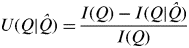 $U(Q|\hat Q) = \displaystyle{{I(Q) - I(Q|\hat Q)} \over {I(Q)}}$.
IV. Quality Against a Benchmark Lexicon
We previously supposed that we had deconstructed the wine note in some way, categorizing the wine descriptors into various levels of detail. To develop a consistent and meaningful wine note metric, we must fix our method of deconstruction. To do this, we require a standard system of categorized wine descriptors. Well-known systems of descriptors include the “Aroma Wheel” (Noble et al., Reference Noble, Arnold, Buechsenstein, Leach, Schmidt and Stern1987) and the WSET Diploma Wine Lexicon (Wine & Spirit Education Trust, 2012). Here we adopt the detailed list of tasting vocabulary in the WSET Diploma Wine Lexicon. However, the methods are entirely adaptable to any system of descriptors, as long as it categorizes the vocabulary according to common attributes. For instance, Ramirez (Reference Ramirez2010) counts the number of wine words from the Wine Spectator's wine word glossary that appear in Napa wine-tasting notes. As an uncategorized list, this glossary is unsuitable for our analysis. However, it should be feasible to build a categorized version of the list. For instance, “delicate” may function as a primary category, which might include the descriptors “subtle,” “floral,” and “perfumed.” We argue that the process of creating a categorized list out of an uncategorized glossary leads to a crystallization of tasting terms and to tasting notes that are more informative.
A. Wine Note Deconstruction
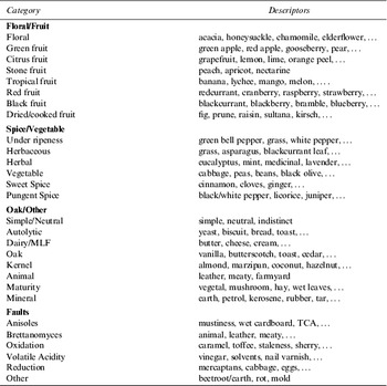
The WSET Diploma Wine Lexicon for aroma and taste characteristics divides descriptors into four main categories each of which then splits into various subcategories, as shown in Table 1. See the WSET website (Wine & Spirit Education Trust, 2012) for full details.
Abbreviated Version of the WSET Diploma Wine Lexicon

Source: Wine & Spirit Education Trust, 2012.
B. The Counting Algorithm
We now introduce the algorithm that breaks down a wine note into its relevant information-theoretic content.
1. Count the number of taste descriptors in each primary category.
2. Count the number of taste descriptors in each secondary category.
(a) If a term in one of the main categories is used but is not further backed up by a detailed descriptor, then the term is counted both as an element of its category and as a descriptor. For instance, a tasting note that includes the term “black fruit” and does not reference any specific examples of black fruit receives one count for the floral/fruit category and one count for the black fruit category. However, if “black fruit” is backed up by “bramble” and “black cherry,” then there is a contribution of two counts to the floral/fruit category and a contribution of two counts to the “black fruit” category.
(b) When a descriptor is used that does not fit into the wine lexicon, we rely on experience as to whether to count the word in one of the categories or to disregard it. Discretion is also required if a descriptor can fall into two different categories. For instance, “animal” could be counted in “Oak/Other” or in “Faults,” depending on the context.
3. List the individual descriptors individually under their respective headings in the secondary category.
Let us deconstruct one of the “randomly generated” tasting in Quandt (Reference Quandt2007) as an example.
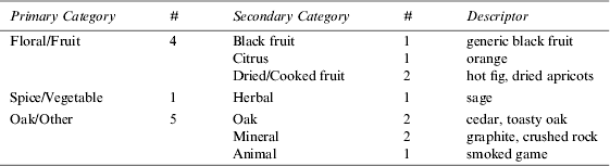
Example 4.1 Château La Merde, 1995Packed and tight, with oily, smoked game and petrol, yet with refined fruit, a hint of black fruit and olive flavors and aromas, and supported by meaty fruit, undergrowth and lush tannins running through the lengthy finish. Best from 2007 through 2025, inky, with olive-tinged black currants, blackberries, tobacco and delicious vegetable flavors.”
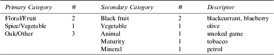
Note that we have not counted “meaty fruit,” as it falls into the main category Floral/Fruit but not into any of the subcategories. If there were no other instances of fruit descriptors, then we could count “meaty fruit” as one instance of “Floral/Fruit” and one instance of one of the subcategories (we would have to use our discretion as to which one). We have not counted “delicious vegetable flavors” because vegetable has been further specified by the term “olive.” We do not double-count, and therefore “olive” contributes only once.
Given a deconstructed tasting note as in the example above, the next task is to calculate a summary statistic based on the Shannon entropy.
V. Calculating the Benchmark Statistic
Let us calculate Shannon information, conditional Shannon information, and uncertainty coefficients for the Château La Merde, 1995, tasting note. We describe the calculations in some detail.
A. Calculations for Château La Merde, 1995
We begin by calculating the quantities I(2) and I(3), respectively defined as the information value of the second and third category of detail in the wine note. The way to understand this in terms of the quiz analogy is as follows: Suppose that your task is to pick a specific wine descriptor from the deconstructed note (which is unknown to you). If you pick the “Vegetable” category, you are done—there is only “olive” left to pick. Thus the information value of “Vegetable” is –log(1/6). But picking “black fruit” gives you an information value of only –log(1/3), because two of the six descriptors are still available, and you must still pick either “blackcurrant” or “blueberry” to end up with a single descriptor. Now, the informational value of the secondary category, I(2), is simply the expected information value in this category. In the language of Definition 3.2, it is the value of asking the omniscient taster (who can see the tasting note) to “reveal the number of descriptors in a secondary category.” To highlight this point of view, we sometimes write I(Q 2) instead of I(2).
Now for the purpose of calculating I(3) (or I(Q 3)), note that if you correctly pick any specific descriptor like “petrol,” you are done immediately; the information value of an isolated descriptor is –log(1/6). Thus, in the terminology of Section 3, all “answers” at this level of detail have the same information content.
Apart from the unconditional information, we need to calculate conditional information in order to produce a statistic based on the uncertainty coefficient. The only difference now is that we calculate information value, given previous information. For instance, given the number of “Oak/Other” descriptors (there are three), what is the remaining information value of picking a descriptor in the secondary category? The calculations are as follows.
Unconditional information: To calculate the unconditional information, we must first calculate the fraction of descriptors that remains after each “answer.”
Let f 1(i) denote the fraction of descriptors in primary category i. In this tasting note, there are three main categories: (1) Floral/Fruit, (2) Spice/Vegetable, and (3) is Oak/Other. We have f 1(1)=1/3, f 1(2)=1/6, and f 1(3)=1/2.
Let f 2(i) denote the fraction of descriptors in secondary category i, where we count from top to bottom in Table 1. First, we have “black fruit,” which contains two descriptors of the total six—that is, a fraction of a third, so f 2(1)=1/3. In the next row, “vegetable” features a single descriptor, so f 2(2)=1/6. Finally, in the “Oak/Other” primary category we have the secondary categories “animal,” “maturity,” and “mineral,” each of which contains a single descriptor compared to the total of six and thus a fraction of 1/6 of the notes” relevant tasting vocabulary. Thus f 2(3)=f 2(4)=f 2(5)=1/6.
Now let f 2(i) be the information associated with revealing one of the descriptors directly. We think again in terms of a quiz, where we are trying to eliminate all but one of the descriptors featured in the tasting notes. It is clear that revealing a descriptor directly eliminates all other remaining options. For instance, finding out that “petrol” is in the tasting note eliminates all but one (petrol) of the six descriptors. Thus, f 3(i)=1/6 for all i.
Next, let I(Q 2), be the Shannon information in asking the omniscient taster to reveal the number of descriptors in a secondary category. Five answers are possible, each with an informational value of –log(f 2(i)), 1 ≤ i ≤5. The probability of answer i is f 2(i), that is the number of descriptors in secondary category i divided by six. The value I(Q 2) of secondary information is, by our earlier definition, simply the expected value of information—that is, the informational value of each answer multiplied by its probability. Thus we have
 $$ I(Q_2 ) = - \sum\limits_{1 \le i \le 5} f_2 (i)\log(\,f_2 (i)) = 1.56.$$
Similarly, let I 3(Q) be the Shannon information of revealing a descriptor. There are six descriptors and we have
 $$.2pt I(Q_3 ) = - \sum\limits_{1 \le i \le 6} f_3 (i)\log(\,f_3 (i)) = 1.79.$$
Conditional Information: Recall Definitions 3.3 and 3.4. To calculate the conditional information, we first calculate I(Q 2|A 1), the conditional information available in the list of secondary descriptors (e.g. black fruit), given knowledge about a primary descriptor (e.g. floral fruit).
Let f 2(i|j) denote the fraction of descriptors remaining with secondary characteristic i (in the primary category j), given knowledge of the number of descriptors in category j. For “black fruit” have f 2(1|1)=1, as all the fruit is black fruit. Similarly, we have f 2(2|2)=1, as all spice/vegetable characteristics are vegetable. Next, f 2(3|3)=f 2(4|3)=f 2(5|3)=1/3 (given the number of Oak/Other characteristics, three different characteristics are left.)
Finally, let f 3(i|j) denote the fraction of descriptors remaining with descriptor i given knowledge of secondary characteristic j. First, given the information that there are two “black fruit” descriptors, we have f 3(1|1)=f 3(2|1)=1/2. Next, there is only one descriptor (olive) in the vegetable category and hence f 3(3|2)=1. Similarly, there is a unique descriptor in each secondary category within “Oak/Other,” whence f 3(4|3)=f 3(5|3)=f 3(6|3)=1.
Now let I(2|1) denote the conditional Shannon information in the second category, given information in the primary category. Note that we have already calculated the probabilities p i in Definition 3.4, which are simply the proportions of descriptors in the three main categories, f 1(1), f 1(2), and f 1(3). Thus we calculate
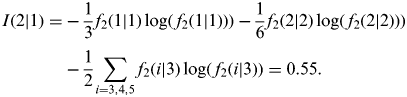 $$\eqalign{ I(2|1) = & - \displaystyle{1 \over 3}f_2 (1|1)\log(\,f_2 (1|1))) - \displaystyle{1 \over 6}f_2 (2|2)\log(\,f_2 (2|2))) \cr & - \displaystyle{1 \over 2}\sum\limits_{i = 3,4,5} f_2 (i|3)\log(\,f_2 (i|3)) = 0.55.} $$
Similarly let I(3|2) denote the conditional Shannon information in the third category, given information in the secondary category. Then we have
 $$\eqalign{I(3|2) = & - \displaystyle{1 \over 3}\sum\limits_{i = 1,2} f_3 (i|1)\log(\,f\,(i|1)) - \displaystyle{1 \over 6}f_3 (3|2)\log(\,f_3 (3|2)) \cr & - \displaystyle{1 \over 6}\sum\limits_{i = 4,5,6} f_3 (i|3)\log(\,f_3 (i|3)) = 0.23.} $$
Remark 5.1For the purpose of developing intuition, we have worked directly from the definition to derive the quantities I (2|1) and I(3|2). In fact, in our wine note setup, it is easy to show that I (2|1)=I(2) – I(1) and I(3|2)=I(3) – I(2) (see Appendix). Thus the calculations are significantly simplified in practice.
B. The Summary Statistic
Definition 5.2The Wine Note Redundancy Statistic (WNRS) is (U(2|1), U(3|2)), where 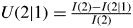 $U(2|1) = {\textstyle{{I(2) - I(2|1)} \over {I(2)}}}$and
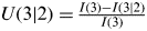 $U(3|2) = {\textstyle{{I(3) - I(3|2)} \over {I(3)}}}$.
In Example 4.1, the WNRS is (0.65, 0.87), since  ${\textstyle{{I(2) - I(2|1)} \over {I(2)}}} = {\textstyle{{1.56 - 0.55} \over {1.56}}} = 0.65$ and
 ${\textstyle{{I(3) - I(3|2)} \over {I(3)}}} = {\textstyle{{1.79 - 0.23} \over {1.79}}} = 0.87$. The WNRS indicates the amount of information that remains to be discovered in Category 2 (resp. Category 3), given knowledge of Category 1 (resp. Category 2). A small redundancy value of U (2|1) indicates that the wine note backs up its primary descriptions with more detailed information at the second level. Similarly, a low value of U (3|1) indicates that second-level information is backed up by a list of detailed attributes. High values (closer to 1) indicate that the writer has not written at a high level of detail. However, extremely low values may indicate that the writer is going into excessive detail in at least one of the categories.
We will now test the relevance of these statistics using the remaining wine notes given by Quandt (Reference Quandt2007). There are three real wine notes and three randomly generated notes, the first of which we have already analyzed.
VI. Real Versus Fake: An Analysis of Wine Notes
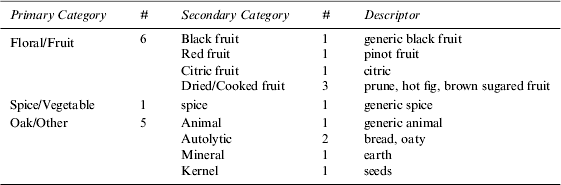
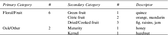
Quandt lists three real tasting notes (1) 1959 A. Ligeret Santenay Gravières, (2) 1995 d'Yquem, Sauternes, (3) 2003 Châteauneuf du Pape Clos du Mont Olivet “Cuvée des Papes,” and three fake tasting notes (4) Château La Merde, 1995, (5) Château Grand-Cul Poilu Coteneuve, 1998, and (6) Château l'Ordure Pomerol, 2004. The summary statistics for each of these are as follows.
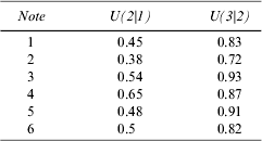
Observe that the genuine notes 1, 2, and 3 tend to perform better than the fake notes. In particular, note 2 for 1995 d'Yquem, Sauternes, has the lowest levels of redundancy and can therefore be considered the best note according to our benchmarked metric. Note 1 also performs relatively well. For instance, while it has a similar level of redundancy in the secondary category as note 5, its level of redundancy at the third level is lower.
However, note 3 does not score any better than note 5, with a higher redundancy in the secondary category and a similar level of redundancy in the third category. The fact that the worst genuine note is number 3, reflects the fact that this note contains a great number of descriptors, each of which corresponds to unique secondary categories. In terms of information content, it is thus hardly distinguishable from number 5, which contains a similar list of adjectives that generally do not back each other up.
Worst in terms of redundancy at the secondary level is the note for Château La Merde. We do not gain information by being told that both fruit descriptors are “black fruit” descriptors or that there is a single “vegetable” descriptor. At the secondary level, there is information only in the “Oak/Other” category, since the three descriptors all fall into different secondary categories.
VII. Concluding Remarks
We have shown that it is possible to develop a wine note metric benchmarked against a categorized list of wine descriptors. Any glossary of wine words can be categorized into levels of increasing specificity. Given a categorized list of descriptors, we have shown how to calculate a Wine Note Redundancy Statistic (WNRS) based on Theil's uncertainty coefficient. What distinguishes a good note is that descriptors back one another up within categories. This reflects the common sense notion that it is not enough for a note to mention characteristics of “dried fruit,” say. Instead, the wine writer should aim to evoke the nature of the “dried fruit” by listing relevant associations falling within the “dried fruit” category in her tasting system. If there is citrus, is it really enough to say “lemon” or is there perhaps also a hint of “orange”? The more internally consistent detail, the lower the redundancy scores, the better the WNRS score.
Wine writers may find it useful to categorize their wine descriptors and make these available alongside their tasting notes. Categorization of tasting terms is a prerequisite for the calculation of redundancy statistics, such as the one presented here. Categorization of wine jargon leads to informative tasting notes.
Appendix
A. Proof that I(2|1)=I(2) – I(1)
In the language of information theory, this statement means that mutual information is zero (see, e.g., Press et al. [2007]), as all information the first category is explained by the information in the second category.
Note that  $I(2|1) = - \sum _i p_i (\sum _j p_{ij} \log(\,p_{ij} ))$, where p i is the probability of receiving answer  i to the first question, and p ij is the probability of receiving answer A j to the second question given the first answer. It follows that
 $I(2) = - \sum _{ij} p_i p_{ij} \log(\,p_i p_{ij} )$ and hence
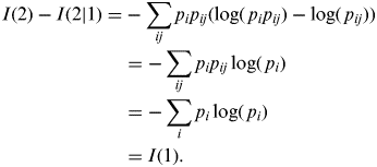 $$\eqalign{I(2) - I(2|1) = & - \sum\limits_{ij} p_i p_{ij} (\log(\,p_i p_{ij} ) - \log(\,p_{ij} )) \cr & = - \sum\limits_{ij} p_i p_{ij} \log(\,p_i ) \cr & = - \sum\limits_i p_i \log(\,p_i ) \cr & = I(1).} $$
The same argument shows that I(3|2)=I(3) – I(2).
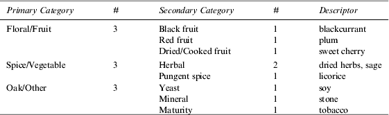
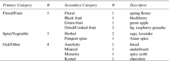
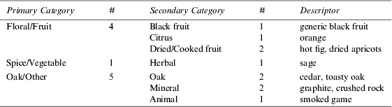
B. Breakdown of the Wine Notes in Quandt (Reference Quandt2007)
1959 A. Ligeret Santenay Gravières
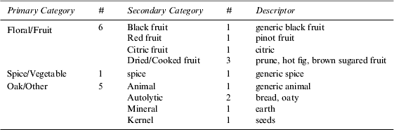
1995 Château d'Yquem, Sauternes
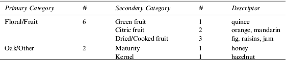
2003 Châteauneuf du Pape Clos du Mont Olivet “Cuvée des Papes”
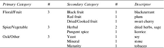
Château Grand-Cul Poilu Coteneuve, 1998
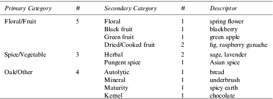
Château l'Ordure Pomerol, 2004