1. Introduction
Turbulent flows, driven by thermal convection and affected by rotation, are ubiquitous phenomena in geo- and astrophysics. Examples are the convection in stars, in the interior of gaseous planets and in the Earth’s atmosphere and oceans, to mention only a few. Even though these phenomena are also shaped by other processes, such as magnetic fields, stratification or liquid–gas phase transition, convection under the influence of the Coriolis force is crucial to their description. Thus to increase our fundamental understanding of the physics behind such flows, we study rotating Rayleigh–Bénard convection, i.e. a fluid rotated about its vertical axis which is heated from below and cooled from above.
The commonly used control parameters of rotating Rayleigh–Bénard convection are the Rayleigh number
 $\mathit{Ra}$
, the Prandtl number
 $\mathit{Pr}$
and the convective Rossby number
 $\mathit{Ro}$
, defined by
 $$\begin{eqnarray}\mathit{Ra}=\frac{{\it\alpha}gH^{3}{\it\Delta}}{{\it\kappa}{\it\nu}},\quad \mathit{Pr}=\frac{{\it\nu}}{{\it\kappa}},\quad \mathit{Ro}=\frac{\sqrt{{\it\alpha}g{\rm\Delta}H}}{2{\it\Omega}H},\end{eqnarray}$$
where
 ${\it\alpha}$
is the isobaric expansion coefficient,
 $g$
the acceleration due to gravity,
 $H$
the vertical distance between the top and bottom plate,
 ${\it\Delta}$
the imposed adverse temperature difference,
 ${\it\kappa}$
the thermal diffusivity,
 ${\it\nu}$
the viscosity and
 ${\it\Omega}$
the angular speed. Instead of
 $\mathit{Ro}$
, occasionally also the Taylor number
 $\mathit{Ta}$
and the Ekman number
 $\mathit{Ek}$
are used to characterise the importance of rotation, which are given by
 $$\begin{eqnarray}\displaystyle & \displaystyle \mathit{Ta}=\left(\frac{2{\it\Omega}H^{2}}{{\it\nu}}\right)^{2}=\frac{\mathit{Ra}}{\mathit{Pr }\mathit{ Ro }^{2}}, & \displaystyle\end{eqnarray}$$
 $$\begin{eqnarray}\displaystyle & \displaystyle \mathit{Ek}=\frac{{\it\nu}}{2{\it\Omega}H^{2}}=\mathit{Ro}\mathit{Pr}^{1/2}\mathit{Ra}^{-1/2}=\mathit{Ta}^{-1/2}. & \displaystyle\end{eqnarray}$$
 ${\it\Gamma}=D/H$
. From the numerical viewpoint an infinite extent can be realised by periodic boundary conditions. This geometry continues to be actively studied (e.g. Hartlep, Tilgner & Busse Reference Hartlep, Tilgner and Busse2003; Sprague et al.
Reference Sprague, Julien, Knobloch and Werne2006; Kunnen, Geurts & Clercx Reference Kunnen, Geurts and Clercx2009; King, Stellmach & Aurnou Reference King, Stellmach and Aurnou2012; Ostilla-Mónico et al.
Reference Ostilla-Mónico, van der Poel, Kunnen, Verzicco and Lohse2014). However, there is also a more recent development in numerical and experimental studies towards smaller and smaller
 ${\it\Gamma}$
of 0.5 (Ahlers et al.
Reference Ahlers, He, Funfschilling and Bodenschatz2012; He et al.
Reference He, Funfschilling, Nobach, Bodenschatz and Ahlers2012) or even 0.23 (Stevens, Lohse & Verzicco Reference Stevens, Lohse and Verzicco2011) with the aim of studying highly turbulent thermal convection, including the transition to the so-called ‘ultimate state’ (Grossmann & Lohse Reference Grossmann and Lohse2011). Thus, the aim is to achieve high
 $\mathit{Ra}$
and, hence, practical considerations demand a small
 ${\it\Gamma}$
. The development to smaller
 ${\it\Gamma}$
also includes rotating convection (Oresta, Stringano & Verzicco Reference Oresta, Stringano and Verzicco2007; Stevens, Clercx & Lohse Reference Stevens, Clercx and Lohse2012; Ecke & Niemela Reference Ecke and Niemela2014). Yet, the finite size has serious implications for rotating Rayleigh–Bénard convection. Not only does the destabilising effect of the lateral wall yield a lower critical
 $\mathit{Ra}$
for the onset of convection at fast rotation rates (Buell & Catton Reference Buell and Catton1983) because of drifting wall modes (Zhong, Ecke & Steinberg Reference Zhong, Ecke and Steinberg1991; Ecke, Zhong & Knobloch Reference Ecke, Zhong and Knobloch1992; Goldstein et al.
Reference Goldstein, Knobloch, Mercader and Net1993, Reference Goldstein, Knobloch, Mercader and Net1994; Herrmann & Busse Reference Herrmann and Busse1993; Kuo & Cross Reference Kuo and Cross1993), but
 ${\it\Gamma}$
also determines the bifurcation point
 $\mathit{Ro}_{b}$
, at which, for
 $\mathit{Pr}\gtrsim 1$
and higher
 $\mathit{Ra}$
, heat transfer enhancement sets in (Weiss et al.
Reference Weiss, Stevens, Zhong, Clercx, Lohse and Ahlers2010; Weiss & Ahlers Reference Weiss and Ahlers2011a
).
The increased heat transport, expressed in terms of the Nusselt number
 $\mathit{Nu}$
, is usually used as an indicator for the different turbulent states occurring in rotating turbulent thermal convection, suggesting a division into three regimes (Kunnen et al.
Reference Kunnen, Stevens, Overkamp, Sun, van Heijst and Clercx2011). In the weak rotation regime,
 $\mathit{Nu}$
remains nearly constant, but as soon as
 $1/\mathit{Ro}$
is increased to values above
 $1/\mathit{Ro}_{b}$
, after a sharp onset, a continuous increase of
 $\mathit{Nu}$
is observed for moderate rotation rotates, which coincides with the generation of columnar vortex structures (Weiss et al.
Reference Weiss, Stevens, Zhong, Clercx, Lohse and Ahlers2010; Stevens et al.
Reference Stevens, Lohse and Verzicco2011). After
 $\mathit{Nu}$
has reached a peak, which marks the transition to the regime of strong rotation, it drops rapidly with the rotation rate due to the suppression of vertical velocity fluctuations (cf. also the recent review by Stevens, Clercx & Lohse Reference Stevens, Clercx and Lohse2013). However, this classification of regimes is only valid for fluids with
 $\mathit{Pr}\gtrsim 1$
; for
 $\mathit{Pr}\lesssim 1$
no heat transfer enhancement is expected (Stevens, Clercx & Lohse Reference Stevens, Clercx and Lohse2010b
).
As the change of
 $\mathit{Nu}$
is closely connected to the columnar vortices, the number of vortices serves as another criterion to determine the point where rotation prevails over. However, extracting these vortices is relatively cumbersome, and involves a certain arbitrariness in choosing what constitutes a vortex. Furthermore, for
 $\mathit{Pr}<1$
the larger diffusivity results in only short vortices that dissipate quickly when they reach the bulk, which complicates matters. Alternatively, one can also look at the large-scale circulation (LSC) or more specifically at the rotation rate when it breaks down (Kunnen, Clercx & Geurts Reference Kunnen, Clercx and Geurts2008; Weiss & Ahlers Reference Weiss and Ahlers2011b
; Stevens et al.
Reference Stevens, Clercx and Lohse2012). In experiments, this information is frequently obtained by analysing the temperature signal at the sidewall. However, one has to be careful with two-vortex states or multiple-roll states occurring in Rayleigh–Bénard cells with small aspect ratios. Evidently, also the crossover of the boundary layer thicknesses (Rossby Reference Rossby1969; King et al.
Reference King, Stellmach, Noir, Hansen and Aurnou2009, Reference King, Stellmach and Aurnou2012) cannot be applied to fluids with
 $\mathit{Pr}<1$
, where the thermal boundary layer is thicker than the viscous one even without rotation.
Here, we offer an alternative method for the characterisation of the different regimes in rotating Rayleigh–Bénard convection. Motivated by the work by Breuer et al. (Reference Breuer, Wessling, Schmalzl and Hansen2004), who have shown that the toroidal and poloidal energy are characteristic for the distinctive types of dynamics in low- and high-Prandtl-number flows in non-rotating convection, namely that the toroidal energy is highest for fluids with
 $\mathit{Pr}\lesssim 1$
(Breuer et al.
Reference Breuer, Wessling, Schmalzl and Hansen2004), and vanishes for
 $\mathit{Pr}=\infty$
(Busse Reference Busse1967), we analyse the contribution of the toroidal and poloidal energy in rotating convection. This is a very natural approach. The poloidal energy is the energy contained in cellular or roll motion, such as the LSC or double-roll states, i.e. the dominant motion without rotation. The toroidal energy, on the other hand, is contained in swirling motion in the horizontal plane, i.e. with a vertical vorticity (Olson & Bercovici Reference Olson and Bercovici1991), which is the dominant motion in rotating convection. This means that we are able to distinguish different regimes of rotating convection based on global quantities, namely the time- and volume-averaged toroidal and poloidal energy, without a restriction to certain Prandtl numbers or aspect ratios.
2. Numerical method
We study rotating Rayleigh–Bénard convection by means of direct numerical simulations (DNS) using a fourth-order finite volume code for cylindrical domains. Details about the code can be found in Shishkina & Wagner (Reference Shishkina and Wagner2005) and Horn, Shishkina & Wagner (Reference Horn, Shishkina and Wagner2013). Additionally, we implemented a term describing the Coriolis force, whereas the centrifugal potential can be incorporated in the reduced pressure and, hence, does not need to be considered explicitly.
We neglect any effects due to centrifugal buoyancy whose importance can be estimated by calculating the Froude number
 $$\begin{eqnarray}\mathit{Fr}=\frac{{\it\Omega}^{2}D}{2g}=\frac{\mathit{Ra}{\it\Gamma}}{8\mathit{Ro}^{2}}\frac{{\it\kappa}{\it\nu}}{gH^{3}}.\end{eqnarray}$$
Since numerically dimensionless equations are solved, we use the parameters of the high-pressure convection facility (HPCF) at the Max Planck Institute for Dynamics and Self-Organization in Göttingen, Germany, to evaluate
 $\mathit{Fr}$
. It is a cylindrical cell, with a height of
 $H=2.24\ \text{m}$
and a diameter of
 $D=1.12\ \text{m}$
, i.e.
 ${\it\Gamma}=1/2$
, filled with sulphur hexafluoride (
 $\text{SF}_{6}$
) at pressures between 2 and 19 bar (Ahlers et al.
Reference Ahlers, He, Funfschilling and Bodenschatz2012; He et al.
Reference He, Funfschilling, Nobach, Bodenschatz and Ahlers2012). At a pressure of 2 bar, the viscosity of
 $\text{SF}_{6}$
is given by
 ${\it\nu}=1.2\times 10^{-6}\ \text{m}^{2}\ \text{s}^{-1}$
and its thermal diffusivity by
 ${\it\kappa}=1.6\times 10^{-6}\ \text{m}^{2}\ \text{s}^{-1}$
, i.e.
 $\mathit{Pr}\approx 0.8$
. The gravitational acceleration in Göttingen is approximately
 $9.81\ \text{m}\ \text{s}^{-2}$
. Thus, for the highest
 $\mathit{Ra}$
and
 $1/\mathit{Ro}$
, namely
 $10^{9}$
and 20, the Froude number is as low as
 $\mathit{Fr}=4.4\times 10^{-4}$
. Hence, since
 $\mathit{Fr}\ll 1$
it is justifiable to set
 $\mathit{Fr}\equiv 0$
(Zhong et al.
Reference Zhong, Stevens, Clercx, Verzicco, Lohse and Ahlers2009). It should be noted that, although the Rayleigh numbers in the HPFC are typically much larger than the ones we can attain in our DNS, an overlap is indeed possible.
The governing equations of the problem are the continuity equation for incompressible flows, the Navier–Stokes equations in Oberbeck–Boussinesq approximation and the energy equation,
 $$\begin{eqnarray}\displaystyle & \boldsymbol{{\rm\nabla}}\boldsymbol{\cdot }\tilde{\boldsymbol{u}}=0, & \displaystyle\end{eqnarray}$$
 $$\begin{eqnarray}\displaystyle & D_{\tilde{t}}\tilde{\boldsymbol{u}}=-\tilde{{\it\rho}}^{-1}\boldsymbol{{\rm\nabla}}\tilde{p}+\tilde{{\it\nu}}{\rm\nabla}^{2}\tilde{\boldsymbol{u}}+2\tilde{{\it\bf\Omega}}\times \tilde{\boldsymbol{u}}+\tilde{g}\tilde{{\it\alpha}}\tilde{T}\hat{\boldsymbol{e}}_{z}, & \displaystyle\end{eqnarray}$$
 $$\begin{eqnarray}\displaystyle & D_{\tilde{t}}\tilde{T}=\tilde{{\it\kappa}}{\rm\nabla}^{2}\tilde{T}, & \displaystyle\end{eqnarray}$$
 $D_{t}$
denotes the substantial derivative,
 $\hat{\boldsymbol{e}}_{z}$
the unit vector in the vertical direction,
 $\boldsymbol{u}$
the velocity,
 $T$
the temperature,
 $p$
the reduced pressure,
 ${\it\bf\Omega}={\it\Omega}\hat{\boldsymbol{e}}_{z}$
the angular velocity and
 ${\it\rho}$
the density. The tilde denotes that the quantity is given in its dimensional representation. However, numerically we solve dimensionless equations in cylindrical coordinates
 $(r,\,{\it\phi},\,z)$
. All variables are replaced by their scaled counterparts, using the radius
 $\hat{R}$
, the buoyancy velocity
 $({\hat{g}}\hat{{\it\alpha}}\hat{R}\hat{{\it\Delta}})^{1/2}$
, the temperature difference
 $\hat{{\it\Delta}}$
and the material properties at the mean temperature as reference scales. The reference time is then given by
 $\hat{R}/({\hat{g}}\hat{{\it\alpha}}\hat{R}\hat{{\it\Delta}})^{1/2}$
and the reference pressure by
 $\hat{{\it\rho}}{\hat{g}}\hat{{\it\alpha}}\hat{R}\hat{{\it\Delta}}$
. In vector notation, the dimensionless governing equations read
 $$\begin{eqnarray}\displaystyle & \boldsymbol{{\rm\nabla}}\boldsymbol{\cdot }\boldsymbol{u}=0, & \displaystyle\end{eqnarray}$$
 $$\begin{eqnarray}\displaystyle & D_{t}\boldsymbol{u}=-\boldsymbol{{\rm\nabla}}p+\mathit{Ra}^{-1/2}\mathit{Pr}^{1/2}{\it\gamma}^{-3/2}{\rm\nabla}^{2}\boldsymbol{u}+\mathit{Ro}^{-1}{\it\gamma}^{1/2}\hat{\boldsymbol{e}}_{z}\times \boldsymbol{u}+T\hat{\boldsymbol{e}}_{z}, & \displaystyle\end{eqnarray}$$
 $$\begin{eqnarray}\displaystyle & D_{t}T=\mathit{Ra}^{-1/2}\mathit{Pr}^{-1/2}{\it\gamma}^{-3/2}{\rm\nabla}^{2}T, & \displaystyle\end{eqnarray}$$
 ${\it\gamma}$
. The sidewall is assumed to be adiabatic and the top and bottom plates are isothermal with
 $T|_{z=H}=T_{t}=-0.5$
and
 $T|_{z=0}=T_{b}=0.5$
. The boundary conditions for the velocity are no-slip at all walls.
All simulations were performed for a fluid with
 $\mathit{Pr}=0.8$
, corresponding to
 $\text{SF}_{6}$
or air, in a slender cylinder with
 ${\it\Gamma}=1/2$
for
 $\mathit{Ra}\in [10^{5},10^{9}]$
and rotation rates
 $1/\mathit{Ro}\in [0,20]$
. The resolution is chosen to fulfil the requirements of Shishkina et al. (Reference Shishkina, Stevens, Grossmann and Lohse2010). The meshes are non-equidistant in the radial and vertical direction, with a clustering of grid points close to the walls. To guarantee enough points in the boundary layers, the grid points were more densely clustered for smaller
 $\mathit{Ro}$
, as it is well-known that the viscous boundary layer becomes thinner as the rotation rate increases (e.g. Kunnen et al.
Reference Kunnen, Clercx and Geurts2008; Stevens, Clercx & Lohse Reference Stevens, Clercx and Lohse2010a
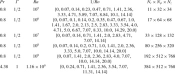
). This means that in the Ekman-type viscous boundary layer in the rotating case the same criterion for the number of grid points was applied as in the non-rotating case. The details of all simulation parameters and the numerical resolution can be found in table 1.
Parameters used in the DNS presented here, including the computational mesh size
 $N_{r}\times N_{{\it\phi}}\times N_{z}$
.

3. Decomposition of the velocity field
In our DNS the Navier–Stokes equations (2.5)–(2.7) are solved in primitive variables, hence in order to obtain the toroidal and poloidal energy we analyse the instantaneous velocity fields every half dimensionless time unit. That means that we decompose the solenoidal velocity field
 $\boldsymbol{u}$
into a poloidal field
 ${\bf\pi}$
and a toroidal field
 ${\bf\tau}$
with the defining scalars
 ${\it\xi}$
and
 ${\it\psi}$
, respectively (Chandrasekhar Reference Chandrasekhar1961; Breuer et al.
Reference Breuer, Wessling, Schmalzl and Hansen2004):
 $$\begin{eqnarray}\boldsymbol{u}={\bf\pi}+{\bf\tau}=\boldsymbol{{\rm\nabla}}\times \boldsymbol{{\rm\nabla}}\times ({\it\xi}\hat{\boldsymbol{e}}_{z})+\boldsymbol{{\rm\nabla}}\times ({\it\psi}\hat{\boldsymbol{e}}_{z}).\end{eqnarray}$$
This decomposition is also called Mie decomposition or Mie representation of the vector field
 $\boldsymbol{u}$
(Backus Reference Backus1986). In cylindrical component notation, (3.1) reads
 $$\begin{eqnarray}\displaystyle & \displaystyle u_{r}={\it\pi}_{r}+{\it\tau}_{r}=\partial _{r}\partial _{z}{\it\xi}+\frac{1}{r}\partial _{{\it\phi}}{\it\psi}, & \displaystyle\end{eqnarray}$$
 $$\begin{eqnarray}\displaystyle & \displaystyle u_{{\it\phi}}={\it\pi}_{{\it\phi}}+{\it\tau}_{{\it\phi}}=\frac{1}{r}\partial _{{\it\phi}}\partial _{z}{\it\xi}-\partial _{r}{\it\psi}, & \displaystyle\end{eqnarray}$$
 $$\begin{eqnarray}\displaystyle & \displaystyle u_{z}={\it\pi}_{z}+{\it\tau}_{z}=-\frac{1}{r}\partial _{r}(r\partial _{r}{\it\xi})-\frac{1}{r^{2}}\partial _{{\it\phi}}\partial _{{\it\phi}}{\it\xi}. & \displaystyle\end{eqnarray}$$
 ${\bf\omega}=\boldsymbol{{\rm\nabla}}\times \boldsymbol{u}$
,
 $$\begin{eqnarray}{\it\omega}_{z}=-\frac{1}{r}\left(\partial _{r}\left(ru_{{\it\phi}}\right)-\partial _{{\it\phi}}u_{r}\right)=-\frac{1}{r}\partial _{r}(r\partial _{r}{\it\psi})-\frac{1}{r^{2}}\partial _{{\it\phi}}\partial _{{\it\phi}}{\it\psi}.\end{eqnarray}$$
The operator
 $-(1/r)\partial _{r}(r\partial _{r})-(1/r^{2})\partial _{{\it\phi}}\partial _{{\it\phi}}\equiv {\it\Delta}_{r{\it\phi}}$
is the horizontal Laplacian. Equations (3.4) and (3.5) are thus two-dimensional Poisson equations
 $$\begin{eqnarray}\displaystyle & {\it\Delta}_{r{\it\phi}}{\it\xi}+u_{z}=0, & \displaystyle\end{eqnarray}$$
 $$\begin{eqnarray}\displaystyle & {\it\Delta}_{r{\it\phi}}{\it\psi}+{\it\omega}_{z}=0. & \displaystyle\end{eqnarray}$$
 ${\it\xi}$
and
 ${\it\psi}$
are not uniquely defined. In fact, to the toroidal potential
 ${\it\psi}$
an arbitrary horizontal harmonic function, i.e. any solution of the corresponding Laplace equation, can be added. The poloidal potential
 ${\it\xi}$
is only determined up to an arbitrary function of
 $z$
(see e.g. Marques et al.
Reference Marques, Net, Massaguer and Mercader1993). Thus, there is a gauge freedom for the boundary conditions. The most simple and commonly used gauge condition for
 ${\it\xi}$
is
 $$\begin{eqnarray}{\it\xi}|_{r=R}=0\end{eqnarray}$$
(Marques et al.
Reference Marques, Net, Massaguer and Mercader1993; Boronski & Tuckerman Reference Boronski and Tuckerman2007). This gauge, in combination with (3.2) and the no-slip condition on the velocity,
 $u_{r}|_{r=R}=0$
, yields
 $$\begin{eqnarray}\partial _{{\it\phi}}{\it\psi}=0.\end{eqnarray}$$
Hence,
 ${\it\psi}$
needs to be constant along the contour
 $r=R$
for a constant
 $z$
and we can also set consistently
 $$\begin{eqnarray}{\it\psi}|_{r=R}=0.\end{eqnarray}$$
Furthermore, we have
 $$\begin{eqnarray}{\it\xi}|_{z=0}={\it\xi}|_{z=H}=0\quad \text{and}\quad {\it\psi}|_{z=0}={\it\psi}|_{z=H}=0\end{eqnarray}$$
(Marques et al.
Reference Marques, Net, Massaguer and Mercader1993). This choice of gauge is the most convenient one, because it implies Dirichlet boundary conditions on
 $r=R$
on the two equations (3.6) and (3.7). Hence, the problem of solving these two Poisson equations becomes well-posed, and the unique solutions for the poloidal and toroidal scalar field are given by
 $$\begin{eqnarray}\displaystyle & \displaystyle {\it\xi}(r,{\it\phi},z)=\int _{0}^{2{\rm\pi}}\int _{0}^{R}u_{z}({\it\zeta},{\it\eta},z)G(r,{\it\phi},{\it\zeta},{\it\eta}){\it\zeta}\text{d}{\it\zeta}\text{d}{\it\eta}, & \displaystyle\end{eqnarray}$$
 $$\begin{eqnarray}\displaystyle & \displaystyle {\it\psi}(r,{\it\phi},z)=\int _{0}^{2{\rm\pi}}\int _{0}^{R}{\it\omega}_{z}({\it\zeta},{\it\eta},z)G(r,{\it\phi},{\it\zeta},{\it\eta}){\it\zeta}\text{d}{\it\zeta}\text{d}{\it\eta}, & \displaystyle\end{eqnarray}$$
 ${\it\zeta}$
and
 ${\it\eta}$
are integration variables and
 $G(r,{\it\phi},{\it\zeta},{\it\eta})$
is the Green’s function
 $$\begin{eqnarray}G(r,{\it\phi},{\it\zeta},{\it\eta})=\frac{1}{4{\rm\pi}}\ln \left(\frac{r^{2}{\it\zeta}^{2}-2R^{2}r{\it\zeta}\cos ({\it\phi}-{\it\eta})+R^{4}}{R^{2}(r^{2}-2r{\it\zeta}\cos ({\it\phi}-{\it\eta})+{\it\zeta}^{2})}\right).\end{eqnarray}$$
Despite the fact that this solution is analytically exact, the large mesh size of the numerically obtained flow fields makes the solving of it computationally expensive and for higher
 $\mathit{Ra}$
, i.e.
 $\mathit{Ra}\gtrsim 10^{8}$
, infeasible. Numerically, it is more efficient to solve the Poisson equations directly. This was done by adapting the well-tested fishpack90 (Swarztrauber & Sweet Reference Swarztrauber and Sweet1975) solver to double precision and our non-equidistant meshes. The solver is based on the generalised Buneman algorithm. Special care is also required at the cylinder axis where in cylindrical coordinates one always faces the problem of the mathematical, but not physical, singularity caused by terms involving
 $1/r$
. But this can be elegantly overcome by calculating (3.12) and (3.13) at
 $r=0$
directly, utilising that the Green’s function in this case simplifies to
 $$\begin{eqnarray}G(0,{\it\phi},{\it\zeta},{\it\eta})=\frac{1}{2{\rm\pi}}\ln \left(\frac{R}{{\it\zeta}}\right).\end{eqnarray}$$
Thus, by prescribing the analytical solution at
 $r=0$
as a numerical boundary condition, a smooth scalar field is guaranteed. It is worth noting that this does not impose any additional physical boundary or gauge condition, but is a direct consequence of the Dirichlet boundary conditions (3.8) and (3.10) and is, hence, merely a numerical trick. Eventually, we are able to calculate the total kinetic energy
 $e_{kin}$
, the poloidal energy
 $e_{pol}$
and the toroidal energy
 $e_{tor}$
, defined by
 $$\begin{eqnarray}\displaystyle & e_{kin}=\langle u_{r}^{2}+u_{{\it\phi}}^{2}+u_{z}^{2}\rangle _{V,t}, & \displaystyle\end{eqnarray}$$
 $$\begin{eqnarray}\displaystyle & e_{pol}=\langle {\it\pi}_{r}^{2}+{\it\pi}_{{\it\phi}}^{2}+{\it\pi}_{z}^{2}\rangle _{V,t}, & \displaystyle\end{eqnarray}$$
 $$\begin{eqnarray}\displaystyle & e_{tor}=\langle {\it\tau}_{r}^{2}+{\it\tau}_{{\it\phi}}^{2}+{\it\tau}_{z}^{2}\rangle _{V,t}, & \displaystyle\end{eqnarray}$$
 $\langle \cdot \rangle _{V,t}$
denotes averaging in time
 $t$
and over the whole volume
 $V$
.
4. Identifying transitions in
 $\text{SF}_{6}$
in a
${\it\Gamma}=1/2$
cell


We propose that the toroidal and poloidal energy can be used to universally capture transitions in rotating Rayleigh–Bénard convection. We present how this method can be applied to thermal convection of a fluid with
 $\mathit{Pr}=0.8$
, corresponding to
 $\text{SF}_{6}$
, that is confined in a slender cylindrical cell with
 ${\it\Gamma}=1/2$
.
4.1. Nusselt number and characteristic flow properties
Most of the recent experiments and numerical simulations on rotating Rayleigh–Bénard convection were conducted in water with
 $3\lesssim \mathit{Pr}\lesssim 7$
(King et al.
Reference King, Stellmach, Noir, Hansen and Aurnou2009; Stevens et al.
Reference Stevens, Zhong, Clercx, Ahlers and Lohse2009; Kunnen, Geurts & Clercx Reference Kunnen, Geurts and Clercx2010; Zhong & Ahlers Reference Zhong and Ahlers2010; Weiss & Ahlers Reference Weiss and Ahlers2011b
). One of the reasons for this might be that only for fluids with
 $\mathit{Pr}>1$
do columnar vortex structures, sometimes called Ekman vortices (Stevens et al.
Reference Stevens, Clercx and Lohse2010b
; Weiss et al.
Reference Weiss, Stevens, Zhong, Clercx, Lohse and Ahlers2010), occur that extend from one horizontal wall to the other (Horn, Shishkina & Wagner Reference Horn, Shishkina and Wagner2011). Via Ekman pumping, the vortices are able to significantly enhance the heat transport compared to the non-rotating case, where the heat flux is usually expressed in terms of the Nusselt number,
 $$\begin{eqnarray}\mathit{Nu}=\left(\mathit{Ra}\mathit{Pr}{\it\gamma}\right)^{1/2}\langle u_{z}T\rangle -{\it\gamma}^{-1}\left\langle \partial _{z}T\right\rangle .\end{eqnarray}$$
But for fluids with
 $\mathit{Pr}<1$
, these vortices are much shorter, and do not form a regular grid. The reason is that the thermal diffusivity is larger than the kinematic viscosity, thus heat can spread in the bulk, making Ekman pumping less effective (Stevens et al.
Reference Stevens, Clercx and Lohse2010b
). Stevens et al. (Reference Stevens, Clercx and Lohse2010b
) found no heat transfer enhancement at all for
 $\mathit{Pr}=0.7$
,
 $\mathit{Ra}=10^{8}$
,
 $0.1\leqslant 1/\mathit{Ro}\leqslant 10.0$
and
 ${\it\Gamma}=1.0$
; however, Oresta et al. (Reference Oresta, Stringano and Verzicco2007) found a slightly higher
 $\mathit{Nu}$
for very similar simulation parameters,
 $\mathit{Pr}=0.7$
,
 $\mathit{Ra}=2\times 10^{8}$
,
 $0.1\leqslant 1/\mathit{Ro}\leqslant 33.3$
but
 ${\it\Gamma}=0.5$
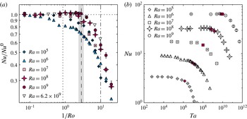
, which they attributed to Ekman pumping. Figure 1(a) shows the Nusselt number for the rotating case normalised by that in the non-rotating case,
 $\mathit{Nu}/\mathit{Nu}^{0}$
, for our DNS for
 $10^{5}\leqslant \mathit{Ra}\leqslant 10^{9}$
and
 $0.07\leqslant 1/\mathit{Ro}\leqslant 20.0$
. In addition, experimental results by Ecke & Niemela (Reference Ecke and Niemela2014) for
 $\mathit{Ra}=6.2\times 10^{9}$
in a cylindrical convection cell with
 ${\it\Gamma}=0.5$
and helium with
 $\mathit{Pr}=0.7$
are shown for comparison. The Nusselt number
 $\mathit{Nu}$
is also presented in figure 1(b), but as function of the Taylor number.
(a) Nusselt number for the rotating case normalised by that for the non-rotating case
 $\mathit{Nu}/\mathit{Nu}^{0}$
as a function of the inverse Rossby number
 $1/\mathit{Ro}$
for
 $\mathit{Ra}\in \{10^{5},10^{6},10^{7},10^{8},10^{9}\}$
obtained by DNS; experimental data by Ecke & Niemela (Reference Ecke and Niemela2014) for
 $\mathit{Ra}=6.2\times 10^{9}$
and
 $\mathit{Pr}=0.7$
are shown for comparison. The vertical dotted line shows the prediction by Weiss et al. (Reference Weiss, Stevens, Zhong, Clercx, Lohse and Ahlers2010) and Weiss & Ahlers (Reference Weiss and Ahlers2011a
),
 $1/\mathit{Ro}_{b}=0.86$
; the vertical long-dashed and dashed-dotted lines mark the transitions proposed by Ecke & Niemela (Reference Ecke and Niemela2014) at
 $1/\mathit{Ro}_{1}\approx 2.86$
and
 $1/\mathit{Ro}_{2}\approx 10.0$
, respectively. The grey shaded area shows where
 $e_{pol}\approx e_{tor}$
at
 $2.36\lesssim 1/\mathit{Ro}_{cr}\lesssim 3.33$
. See also table 2 in § 6 for the definitions of the
 $1/\mathit{Ro}$
marking the regime borders. (b) Nusselt number
 $\mathit{Nu}$
as function of the Taylor number
 $\mathit{Ta}$
. The filled (pink online) symbols show where
 $e_{pol}\approx e_{tor}$
and are the same as marked by the grey shaded area in (a).

For
 $\mathit{Ra}=10^{5}$
, we have steady convection for all Rossby numbers considered, except for
 $1/\mathit{Ro}=14.1$
, where convection is completely suppressed due to rotation and heat is transported by conduction alone. For
 $\mathit{Ra}=10^{6}$
, convection is chaotic and unsteady for
 $1/\mathit{Ro}\lesssim 1.67$
, while for
 $1.67\gtrsim 1/\mathit{Ro}\gtrsim 2.5$
we found oscillatory convection and for even faster rotation rates, i.e.
 $1/\mathit{Ro}\gtrsim 2.5$
, convection is steady. For
 $\mathit{Ra}=10^{7}$
, we have turbulent convection for low rotation rates, but again, however, for even faster rotation rates, i.e.
 $1/\mathit{Ro}=14.1$
, we observed steady convection. Finally, for
 $\mathit{Ra}=10^{8}$
and
 $\mathit{Ra}=10^{9}$
our applied rotation was never rapid enough to completely suppress turbulent fluctuations.
The general behaviour of
 $\mathit{Nu}$
with increasing rotation rate is very similar for all
 $\mathit{Ra}$
, i.e. it is almost constant for slow rotation and then drops rapidly at a certain rotation rate. There is also a very slightly increased
 $\mathit{Nu}$
for
 $1/\mathit{Ro}\lesssim 2$
, which is due to the stabilising effect of rotation, which suppresses reversals and changes from a one-roll state to a double-roll state, that occur more frequently for
 ${\it\Gamma}=0.5$
than for
 ${\it\Gamma}=1.0$
. For
 $\mathit{Ra}=10^{6}$
there is more switching between these different states than for the other
 $\mathit{Ra}$
, which is a possible explanation for the evident deviation of the behaviour of the Nusselt number for that particular Rayleigh number. This was also found by Oresta et al. (Reference Oresta, Stringano and Verzicco2007), in numerical simulations with parameters very similar to ours at
 $\mathit{Ra}=9\times 10^{5}$
and
 $\mathit{Pr}=0.7$
. The continuous decrease of
 $\mathit{Nu}$
with increasingly high rotation rate is expected from the Taylor–Proudman theorem (Proudman Reference Proudman1916; Taylor Reference Taylor1921), which predicts the suppression of flow variations along the axis of rotation. Although strictly speaking the Taylor–Proudman theorem is not applicable to the highly nonlinear and time-dependent case of rotating Rayleigh–Bénard convection, the reduced heat transport can be understood in terms of it.
In figure 1(a) the prediction by Weiss et al. (Reference Weiss, Stevens, Zhong, Clercx, Lohse and Ahlers2010) and Weiss & Ahlers (Reference Weiss and Ahlers2011a
) based on a phenomenological Ginzburg–Landau model is also shown. They have shown that for fluids with
 $\mathit{Pr}\gtrsim 1$
, at
 $$\begin{eqnarray}\frac{1}{\mathit{Ro}_{b}}=\frac{a}{{\it\Gamma}}\left(1+\frac{b}{{\it\Gamma}}\right),\quad a=0.381,b=0.061\end{eqnarray}$$
a bifurcation corresponding to the onset of Ekman vortex formation and Nusselt number enhancement occurs. This bifurcation is a finite-size effect, and gives
 $1/\mathit{Ro}_{b}=0.86$
for
 ${\it\Gamma}=0.5$
.
For
 $\mathit{Pr}=0.8$
and
 $\mathit{Ra}=10^{5}$
and
 $\mathit{Ra}=10^{7}$
the Nusselt number starts to decrease at the point
 $1/\mathit{Ro}_{b}$
, but no columnar vortices were observed. However, for
 $\mathit{Ra}=10^{8}$
and
 $\mathit{Ra}=10^{9}$
, we found short columnar vortices and the Nusselt number also appears to increase slightly and then drops at a critical inverse Rossby number
 $2.36\lesssim 1/\mathit{Ro}_{cr}\lesssim 3.33$
. In figure 1(a) this rotation rate is indicated by a grey shaded area, while in figure 1(b), where
 $\mathit{Nu}$
is plotted against
 $\mathit{Ta}$
, it corresponds to the filled symbols. The transition at
 $1/\mathit{Ro}_{cr}$
is consistent with the one found empirically by Ecke & Niemela (Reference Ecke and Niemela2014) at
 $1/\mathit{Ro}_{1}\approx 2.86$
. Furthermore, Ecke & Niemela (Reference Ecke and Niemela2014) suggested that after this initial decrease a more rapid decrease occurs after
 $1/\mathit{Ro}_{2}\approx 10.0$
. An accurate identification of
 $\mathit{Ro}_{cr}$
solely based on the Nusselt number is nonetheless difficult.
That a transition in the flow occurs is also visible in other important flow characteristics such as the radial velocity component
 $u_{r}$
, the temperature
 $T$
, the r.m.s. temperature
 $T_{rms}$
or the skewness of the temperature
 $S_{T}$
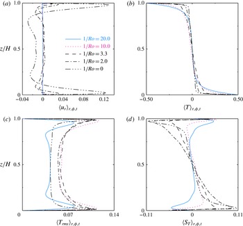
. The temporally, radially and azimuthally averaged profiles of these quantities are presented in figure 2 for five representative rotation rates,
 $1/\mathit{Ro}\in \{0,2.0,3.3,10.0,20.0\}$
. To rule out the sidewall effects (Kunnen, Clercx & van Heijst Reference Kunnen, Clercx and van Heijst2013), the radial averaging was performed for
 $0\leqslant r\leqslant 0.9R$
(Stevens et al.
Reference Stevens, Clercx and Lohse2010a
). All of them, but in particular the radial velocity and the skewness of the temperature, reveal a significant flow change for
 $1/\mathit{Ro}\gtrsim 3.3$
.
Temporally, radially and azimuthally averaged profiles of (a) the radial velocity component
 $u_{r}$
, (b) the temperature
 $T$
, (c) the r.m.s. temperature
 $T_{rms}$
and (d) the skewness of the temperature
 $S_{T}$
for
 $\mathit{Ra}=10^{8}$
. The radial averaging was performed for
 $0\leqslant r\leqslant 0.9R$
.

The radial velocity
 $u_{r}$
as function of the vertical coordinate
 $z$
, figure 2(a), nicely demonstrates the Taylor–Proudman effect. Variations of the flow in the vertical direction are inhibited and as a consequence roll-like structures such as the LSC are not permitted. Hence, while the
 $u_{r}$
mean profiles at low rotation rates still show the typical shape reflecting these structures, they no longer show any variation in the bulk as soon as these structures break down. The first three moments of the temperature, presented in figure 2(b–d), reflect the impact of the generated columnar vortices. The mean temperature profiles exhibit a non-zero gradient in the bulk increasing with
 $1/\mathit{Ro}$
and strongest close to the plates. This is usually attributed to vortex merger (Julien et al.
Reference Julien, Legg, McWilliams and Werne1996). However, even without rotation a small non-vanishing temperature gradient is present that we assume to be due to the small aspect ratio. The r.m.s. temperature also varies significantly with the rotation rate. It is almost constant without rotation, showing a crescent-shaped profile up to
 $1/\mathit{Ro}\approx 10.0$
. For
 $1/\mathit{Ro}=20.0$
, the crescent-shape is dented in the midplane and bent in the opposite direction. The skewness of the temperature also exhibits signs of a fundamental change in the flow, in particular close to the vicinity of the top and bottom plates: with increasing
 $1/\mathit{Ro}$
,
 $S_{T}$
abruptly changes sign at
 $1/\mathit{Ro}\approx 10.0$
. A similar change of behaviour was also reported by Kunnen, Clercx & Geurts (Reference Kunnen, Clercx and Geurts2006) and Kunnen et al. (Reference Kunnen, Geurts and Clercx2009) for the skewness of the vertical velocity
 $S_{u_{z}}$
and of the r.m.s. vorticity
 $S_{{\it\omega}_{z}}$
, obtained by simulations in a periodic domain, for
 $\mathit{Pr}=1$
and
 $\mathit{Ra}=2.5\times 10^{6}$
.
4.2. Toroidal and poloidal potential and energy
In the following we show how to connect the different flow behaviour with the toroidal and poloidal potential and energy. It will allow us to effectively identify the transitions between different regimes in rotating Rayleigh–Bénard based on the global quantities
 $e_{tor}$
and
 $e_{pol}$
.
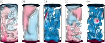
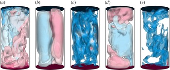
In figures 3–7 we present instantaneous flow quantities for the same representative rotation rates
 $1/\mathit{Ro}\in \{0,2.0,3.3,10.0,20.0\}$
at
 $\mathit{Ra}=10^{8}$
as before. We refrain from showing averaged flow fields, since the precession motion of the flow might distort their interpretation.
Instantaneous flow structures for
 $\mathit{Ra}=10^{8}$
and
 $1/\mathit{Ro}=0$
, i.e. without rotation. Shown are twelve isosurfaces that are equidistantly distributed between the interval boundaries. Colour scale ranges from blue (the smallest value) through white to pink (the largest value): (a) temperature
 $T\in [-0.5,0.5]$
; (b) poloidal potential
 ${\it\xi}\in [-0.04,0.04]$
; (c) poloidal energy
 $e_{pol}\in [0,0.76]$
; (d) toroidal potential
 ${\it\psi}\in [-0.13,0.13]$
; (e) toroidal energy
 $e_{tor}\in [0,0.27]$
.

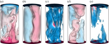
As in figure 3, but for
 $1/\mathit{Ro}=2.0$
: (a) temperature
 $T\in [-0.5,0.5]$
; (b) poloidal potential
 ${\it\xi}\in [-0.03,0.03]$
; (c) poloidal energy
 $e_{pol}\in [0,0.70]$
; (d) toroidal potential
 ${\it\psi}\in [-0.16,0.16]$
; (e) toroidal energy
 $e_{tor}\in [0,0.74]$
.

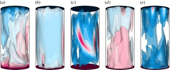
As in figure 3, but for
 $1/\mathit{Ro}=3.3$
: (a) temperature
 $T\in [-0.5,0.5]$
; (b) poloidal potential
 ${\it\xi}\in [-0.02,0.02]$
; (c) poloidal energy
 $e_{pol}\in [0,0.27]$
; (d) toroidal potential
 ${\it\psi}\in [-0.21,0.21]$
; (e) toroidal energy
 $e_{tor}\in [0,0.77]$
.

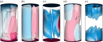
As in figure 3, but for
 $1/\mathit{Ro}=10.0$
: (a) temperature
 $T\in [-0.5,0.5]$
; (b) poloidal potential
 ${\it\xi}\in [-0.003,0.003]$
; (c) poloidal energy
 $e_{pol}\in [0,0.12]$
; (d) toroidal potential
 ${\it\psi}\in [-0.11,0.11]$
; (e) toroidal energy
 $e_{tor}\in [0,0.22]$
.

As in figure 3, but for
 $1/\mathit{Ro}=20.0$
: (a) temperature
 $T\in [-0.5,0.5]$
; (b) poloidal potential
 ${\it\xi}\in [-0.001,0.001]$
; (c) poloidal energy
 $e_{pol}\in [0,0.05]$
; (d) toroidal potential
 ${\it\psi}\in [-0.03,0.03]$
; (e) toroidal energy
 $e_{tor}\in [0,0.09]$
.

In the non-rotating case,
 $1/\mathit{Ro}=0$
(figure 3), the flow is most of the time organised as an LSC. This structure is not only visible in the temperature field
 $T$
but also in the poloidal potential
 ${\it\xi}$
and energy
 $e_{pol}$
. The toroidal potential
 ${\it\psi}$
shows a rather chaotic structure and the toroidal energy
 $e_{tor}$
is concentrated in the bulk and of lower magnitude than
 $e_{pol}$
. If the flow were two-dimensional and independent of one horizontal direction then it would be completely poloidal. However, since the toroidal energy is associated with the vortices in the flow, the toroidal field acts in a destabilising way on the flow and tears the plumes apart. On the other hand, when the convection cell is rotated, the toroidal field has a stabilising effect. With increasing rotation rate, as seen in figures 4–7, the flow resembles a horizontally two-dimensional flow, but a two-dimensional flow independent of the vertical direction is fully toroidal. This means that with increasing
 $1/\mathit{Ro}$
the toroidal energy increases and the poloidal energy decreases. Instead of an LSC, there are elongated flow structures emerging from the edge of the boundary layers, that are visible in the temperature field and in the toroidal potential
 ${\it\psi}$
and energy
 $e_{tor}$
. The highest toroidal energy is contained in these short columnar-like vortices seen in figures 5 and 6. For even more rapid rotation, at
 $1/\mathit{Ro}=20.0$
(figure 7), which is close to the onset of convection, wall modes dominate and both the poloidal and toroidal energy are highest close to the sidewall. Hence, the toroidal and poloidal energy can be used to characterise the different types of dynamics in rotating Rayleigh–Bénard convection.
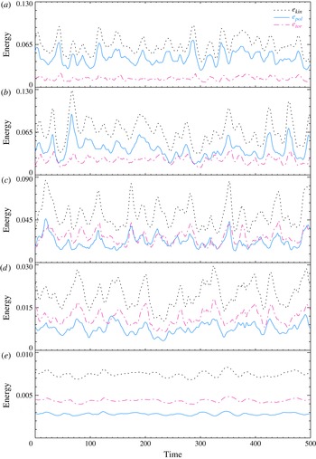
In figure 8 we show the temporal evolution of
 $e_{kin}$
,
 $e_{pol}$
and
 $e_{tor}$
. For
 $1/\mathit{Ro}=0$
and
 $1/\mathit{Ro}=2.0$
it is indeed the case that
 $e_{pol}>e_{tor}$
for all instances of time, while for
 $1/\mathit{Ro}=10.0$
and
 $1/\mathit{Ro}=20.0$
,
 $e_{pol}<e_{tor}$
. For
 $1/\mathit{Ro}=3.3$
,
 $e_{pol}$
and
 $e_{tor}$
are of the same order. Furthermore, the oscillation frequency tends to decrease with increasing
 $1/\mathit{Ro}$
.
Times series of the volume-averaged kinetic energy
 $e_{kin}$
(black dotted line), the poloidal energy
 $e_{pol}$
(solid line, blue online) and the toroidal energy
 $e_{tor}$
(dash-dotted line, pink online) for
 $\mathit{Ra}=10^{8}$
and (a)
 $1/\mathit{Ro}=0$
, (b)
 $1/\mathit{Ro}=2.0$
, (c)
 $1/\mathit{Ro}=3.3$
, (d)
 $1/\mathit{Ro}=10.0$
, (e)
 $1/\mathit{Ro}=20.0$
. The time is measured in dimensionless time units (see main text), and all time series were deliberately set to zero at a point when statistical equilibrium was reached.

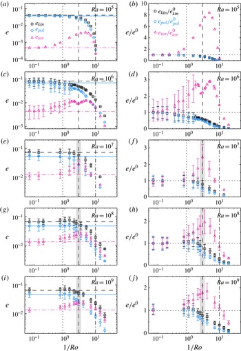
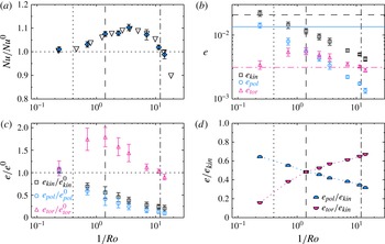
To analyse these observations quantitatively, the volume- and time-averaged energies are shown in figure 9 for all simulations conducted. Similar to figure 1(a), we also compare them with
 $1/\mathit{Ro}_{b}$
suggested by Weiss et al. (Reference Weiss, Stevens, Zhong, Clercx, Lohse and Ahlers2010) and Weiss & Ahlers (Reference Weiss and Ahlers2011a
) and the empirically found
 $1/\mathit{Ro}_{1}$
and
 $1/\mathit{Ro}_{2}$
by Ecke & Niemela (Reference Ecke and Niemela2014).
(a,c,e,g,i) Volume- and time-averaged kinetic energy
 $e_{kin}$
(black squares and dashed line), poloidal energy
 $e_{pol}$
(circles and solid line, blue online) and toroidal energy
 $e_{tor}$
(triangles and dash-dotted line, pink online) as function of
 $1/\mathit{Ro}$
. The horizontal lines indicate the value in the non-rotating case. (b,d,f,h,j) Volume- and time-averaged kinetic energies normalised by their value in the non-rotating case. The vertical dotted lines shows prediction by Weiss et al. (Reference Weiss, Stevens, Zhong, Clercx, Lohse and Ahlers2010) and Weiss & Ahlers (Reference Weiss and Ahlers2011a
),
 $1/\mathit{Ro}_{b}=0.86$
, the vertical long-dashed and dashed-dotted lines mark the transitions proposed by Ecke & Niemela (Reference Ecke and Niemela2014) at
 $1/\mathit{Ro}_{1}\approx 2.86$
and
 $1/\mathit{Ro}_{2}\approx 10.0$
, respectively. The grey shaded areas indicate where
 $e_{pol}\approx e_{tor}$
at
 $2.36\lesssim 1/\mathit{Ro}_{cr}\lesssim 3.33$
. The error bars show the standard deviation
 ${\it\sigma}$
of the averaged values. See also table 2 in § 6.

The DNS data share some common features for all Rayleigh numbers. All energies
 $e_{kin}$
,
 $e_{pol}$
and
 $e_{tor}$
are independent of
 $1/\mathit{Ro}$
up to approximately
 $1/\mathit{Ro}_{b}=0.86$
. At this point,
 $e_{kin}$
and
 $e_{pol}$
decrease monotonically. On the contrary,
 $e_{tor}$
increases at this point, then reaches a maximum and after that drops with increasing
 $1/\mathit{Ro}$
. It reaches the same value as in the non-rotating case at
 $1/\mathit{Ro}_{2}\approx 8.33$
.
For the relatively low Rayleigh numbers
 $\mathit{Ra}=10^{5}$
and
 $\mathit{Ra}=10^{6}$
, the toroidal energy is always lower than the poloidal energy, despite the fact that the toroidal energy can be up to about eight and three times higher, respectively, than in the non-rotating case, as can be seen in figure 9(a–d). As a consequence, the poloidal field is, for all rotation rates, able to sustain cellular-like flow structures. Since for
 $\mathit{Ra}=10^{5}$
convection is steady for all
 $1/\mathit{Ro}$
, the standard deviation
 ${\it\sigma}$
is zero. For
 $\mathit{Ra}=10^{6}$
, convection is unsteady for
 $0\leqslant 1/\mathit{Ro}\lesssim 1.67$
and due to the small computational mesh, DNS could be performed for several thousands of time units. Hence, the large error bars in figure 9(c,d) indicate physical variations and not a lack of statistics. In the range
 $1.67\lesssim 1/\mathit{Ro}\lesssim 2.5$
, when the convective heat transport is oscillatory,
 ${\it\sigma}$
decreases with increasing
 $1/\mathit{Ro}$
. The oscillatory behaviour is naturally present in the time series of
 $e_{kin}$
,
 $e_{pol}$
and
 $e_{tor}$
. For even larger
 $1/\mathit{Ro}$
, we found steady convection, in the sense that the Nusselt number does not change in time. Interestingly, at the transition between oscillatory and steady convection, there is a minimum in the toroidal energy and this point also coincides with
 $1/\mathit{Ro}_{1}$
.
For
 $\mathit{Ra}=10^{7}$
we observed turbulent convection for all
 $1/\mathit{Ro}$
considered, except for the highest rotation rate
 $1/\mathit{Ro}=14.1$
, where convection is steady. But in this case, presented in 9(e, f), the toroidal energy is higher than the poloidal energy for
 $1/\mathit{Ro}$
greater than a critical inverse Rossby number
 $1/\mathit{Ro}_{cr}$
. This critical inverse Rossby number is hence determined by the condition
 $$\begin{eqnarray}\frac{1}{\mathit{Ro}_{cr}}=\left.\frac{1}{\mathit{Ro}}\right|_{e_{pol}=e_{tor}}.\end{eqnarray}$$
We argue that only if toroidal motions are prevailing, i.e.
 $e_{tor}>e_{pol}$
, one can speak of rotation-dominated convection. If, on the other hand, poloidal motions are predominant, i.e.
 $e_{tor}<e_{pol}$
, then buoyancy is more important. If
 $e_{tor}>e_{pol}$
, the LSC or other roll-like structures cease to exist and instead columnar vortices become apparent. Thus, this clarifies the change of behaviour observed in the global flow properties presented in figure 2 and discussed in the previous section. Furthermore, these findings are also in agreement with those by other authors (Kunnen et al.
Reference Kunnen, Clercx and Geurts2008; Stevens et al.
Reference Stevens, Clercx and Lohse2012, Reference Stevens, Clercx and Lohse2013) that relate the breakdown of the LSC to the regime of rotation dominance. They also shed some more light on the fact that not only the inverse Rossby number but also the Rayleigh number has to be sufficiently high to reach a rotation-dominated regime (Julien et al.
Reference Julien, Knobloch, Rubio and Vasil2012; Ecke & Niemela Reference Ecke and Niemela2014). The behaviour of
 $e_{kin}$
,
 $e_{pol}$
and
 $e_{tor}$
with
 $1/\mathit{Ro}$
at
 $\mathit{Ra}=10^{8}$
and
 $\mathit{Ra}=10^{9}$
, displayed in figure 9(g–j), is very similar to that at
 $\mathit{Ra}=10^{7}$
, but the maximum relative enhancement of the toroidal energy compared to the non-rotating case is diminished with higher
 $\mathit{Ra}$
. Nonetheless, in these cases the crossover of the poloidal and toroidal energy is more pronounced, in the sense that the difference between
 $e_{tor}$
and
 $e_{pol}$
is larger at rapid rotation.
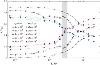
To determine the transition point more accurately, the ratios of the toroidal to the total kinetic energy
 $e_{tor}/e_{kin}$
and of the poloidal to the total kinetic energy
 $e_{pol}/e_{kin}$
are shown in figure 10. The ratios
 $e_{tor}/e_{kin}$
and
 $e_{pol}/e_{kin}$
are known to be properties of the flow characterising the different types of dynamics in non-rotating Rayleigh–Bénard convection (Breuer et al.
Reference Breuer, Wessling, Schmalzl and Hansen2004) and we argue that the same is true for rotating Rayleigh–Bénard convection.
Poloidal and toroidal energy as a fraction of the total kinetic energy versus
 $1/\mathit{Ro}$
. The grey shaded area shows the approximate range where
 $e_{pol}=e_{tor}$
at
 $2.4\lesssim 1/\mathit{Ro}_{cr}\lesssim 3.3$
. The open symbols denote the DNS with Rayleigh numbers where
 $e_{tor}$
is always below
 $e_{pol}$
, i.e.
 $\mathit{Ra}=10^{5}$
and
 $10^{5}$
. The filled symbols denote the DNS with Rayleigh numbers where a crossover of
 $e_{tor}$
and
 $e_{pol}$
occurs, i.e.
 $\mathit{Ra}\in \{10^{7},10^{8},10^{9}\}$
.

Figure 10 reveals various pieces of information. First of all, the critical inverse Rossby number is approximately
 $1/\mathit{Ro}_{cr}\approx 3.0$
or more accurately it lies in the range
 $2.36\lesssim 1/\mathit{Ro}_{cr}\lesssim 3.33$
. At this point, both the poloidal and the toroidal energy are approximately 50 % of the total kinetic energy. From equations (3.2)–(3.4) and (3.16)–(3.18) it is obvious that not all of the kinetic energy is contained in the toroidal and poloidal parts, since
 $$\begin{eqnarray}e_{kin}\neq e_{pol}+e_{tor}.\end{eqnarray}$$
However, as can be readily seen from figure 10, the sum of
 $e_{tor}$
and
 $e_{pol}$
is, for all cases, approximately 90 % of the total kinetic energy, indicating that the single components of the toroidal and poloidal field are almost uncorrelated.
At small inverse Rossby numbers,
 $1/\mathit{Ro}\lesssim 1$
, and also in non-rotating convection, the poloidal energy decreases, and the toroidal energy increases with the Rayleigh number. Without rotation, at
 $\mathit{Ra}=10^{5}$
approximately 90 % of the kinetic energy is contained in the poloidal energy and only approximately 1 % in the toroidal energy. At
 $\mathit{Ra}=10^{9}$
only approximately 70 % of the kinetic energy is contained in the poloidal motion and 20 % in the toroidal energy. This is not surprising, because the higher
 $\mathit{Ra}$
the greater the number of plumes. Hence, there is an increased shearing and swirling in the flow that is associated with a vertical vorticity and a higher
 $e_{tor}$
. Consequently,
 $e_{pol}$
has to decrease. This is also related to the picture of a less strong LSC at higher
 $\mathit{Ra}$
. With increasing
 $1/\mathit{Ro}$
one has to distinguish between the steady cases
 $\mathit{Ra}=10^{5}$
and
 $10^{6}$
and the turbulent cases
 $10^{7}\leqslant \mathit{Ra}\leqslant 10^{9}$
. At intermediate inverse Rossby numbers,
 $1\lesssim 1/\mathit{Ro}\lesssim 5$
,
 $e_{tor}/e_{kin}$
and
 $e_{pol}/e_{kin}$
collapse onto approximately the same value for
 $10^{7}\leqslant \mathit{Ra}\leqslant 10^{9}$
, unlike for
 $10^{5}$
and
 $10^{6}$
. Between
 $7\lesssim 1/\mathit{Ro}\lesssim 10$
the two data sets for
 $\mathit{Ra}=10^{6}$
and
 $10^{7}$
touch each other; however, for
 $\mathit{Ra}=10^{6}$
,
 $e_{tor}/e_{kin}$
subsequently drops to a value of approximately 0.4 at
 $1/\mathit{Ro}=20.0$
and
 $e_{pol}/e_{kin}$
rises again to a value of approximately 0.55. On the contrary, for
 $\mathit{Ra}=10^{7}$
,
 $e_{tor}/e_{kin}$
increases further to 0.53 and
 $e_{pol}/e_{kin}$
decreases to 0.42 at
 $1/\mathit{Ro}=14.1$
. Thus, there is a clear distinction between non-turbulent and turbulent rotating Rayleigh–Bénard convection. Similarly, at large inverse Rossby numbers,
 $1/\mathit{Ro}\gtrsim 5$
, the data show a larger spread depending on the Rayleigh number. At
 $1/\mathit{Ro}\gtrsim 14$
,
 $\mathit{Ra}=10^{5}$
is in the conducting state, hence
 $e_{tor}$
,
 $e_{pol}$
and
 $e_{kin}$
are zero. The relative toroidal energy is highest for
 $\mathit{Ra}=10^{9}$
, being approximately 70 % of the kinetic energy and the poloidal energy is lowest for the same
 $\mathit{Ra}$
, being approximately 29 % at
 $1/\mathit{Ro}=20.0$
.
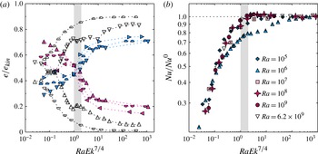
Another way of collapsing the data has been suggested by Ecke & Niemela (Reference Ecke and Niemela2014): choosing the quantity
 $\mathit{Ra}\mathit{Ek}^{7/4}=\mathit{Ra}^{1/8}\mathit{Pr}^{7/8}\mathit{Ro}^{7/4}$
instead of
 $1/\mathit{Ro}$
. This implies a dependence on
 $\mathit{Ra}$
and
 $\mathit{Pr}$
, and indeed figure 11(a) reveals that the collapse onto the critical point where the toroidal and poloidal energy are equal is even better. The crossover determined in this way happens in the range
 $1\leqslant \mathit{Ra}\mathit{Ek}^{7/4}\leqslant 2$
or at
 $\mathit{Ra}\mathit{Ek}^{7/4}\approx 1.5$
, respectively. This quantity was also found to be a suitable scaling variable in water with
 $\mathit{Pr}=7$
(King et al.
Reference King, Stellmach, Noir, Hansen and Aurnou2009), although it was corrected to
 $\mathit{Ra}\mathit{Ek}^{3/2}$
later on (King et al.
Reference King, Stellmach and Aurnou2012). However, the latter does not fit to our data. A better agreement of the
 $\mathit{Nu}$
behaviour for all
 $\mathit{Ra}$
(except for the particularities occurring at
 $\mathit{Ra}=10^{6}$
) when plotted against
 $\mathit{Ra}\mathit{Ek}^{7/4}$
is also obtained and had already been found by Ecke & Niemela (Reference Ecke and Niemela2014). It is presented in figure 11(b).
(a) Poloidal and toroidal energy as a fraction of the total kinetic energy versus
 $\mathit{Ra}\mathit{Ek}^{7/4}$
. Similar to figure 10, and with the same meanings for the symbols. The grey shaded area shows the approximate range where
 $e_{pol}=e_{tor}$
at
 $1.0\lesssim \mathit{Ra}\mathit{Ek}_{cr}^{7/4}\lesssim 2.0$
. (b) Nusselt number for the rotating case normalised by that for the non-rotating case
 $\mathit{Nu}/\mathit{Nu}^{0}$
as function of
 $\mathit{Ra}\mathit{Ek}^{7/4}$
. Similar to figure 1(a).

5. Identifying transitions in water in a
${\it\Gamma}=1$
cell

It is evident from the mathematical formulation that the proposed method works independently of the Prandtl number and the aspect ratio. We corroborate this by applying the analysis to a fluid with
 $\mathit{Pr}=4.38$
, corresponding to water, confined in a cylindrical cell with an aspect ratio of
 ${\it\Gamma}=1$
. The Rayleigh number is
 $\mathit{Ra}=1.16\times 10^{9}$
allowing a direct comparison to the experimental data by Kunnen et al. (Reference Kunnen, Stevens, Overkamp, Sun, van Heijst and Clercx2011). Kunnen et al. (Reference Kunnen, Stevens, Overkamp, Sun, van Heijst and Clercx2011) have also shown that their data are in agreement with the measurements by Zhong & Ahlers (Reference Zhong and Ahlers2010) at almost the same Rayleigh number of
 $\mathit{Ra}=1.2\times 10^{9}$
. Here we only briefly discuss the relevant results. More details about the water simulations are reported in Horn & Shishkina (Reference Horn and Shishkina2014).
In the case of water also, the first emergence of columnar vortex structures and the increase of the toroidal energy coincide. But in addition a pronounced heat transfer enhancement is found that sets in at the same point. This can be readily seen in figure 12(a–c) where the normalised Nusselt number
 $\mathit{Nu}/\mathit{Nu}^{0}$
, the absolute value of
 $e_{kin}$
,
 $e_{pol}$
and
 $e_{tor}$
, and the normalised energies
 $e_{kin}/e_{kin}^{0}$
,
 $e_{pol}/e_{pol}^{0}$
and
 $e_{tor}/e_{tor}^{0}$
are presented. The inverse Rossby number for this point can again be determined by (4.2) yielding
 $1/\mathit{Ro}=0.40$
for the case of
 ${\it\Gamma}=1$
. Figure 12 also reveals that the rotation rate
 $1/Ro$
where the heat transfer
 $\mathit{Nu}$
and where the toroidal energy
 $e_{tor}$
drop below their respective reference values obtained without rotation match identically. It is determined to be
 $1/\mathit{Ro}_{2}\approx 12.0$
. This agreement is expected since it is known that for larger Prandtl numbers the heat transfer enhancement scales with the number of columnar vortex structures at the height of the boundary layer (Liu & Ecke Reference Liu and Ecke2009) and these again correlate with the toroidal energy.
Additional data showing the applicability of the method to higher Prandtl numbers and aspect ratios for the example of a fluid with
 $\mathit{Pr}=4.38$
; the Rayleigh number is
 $\mathit{Ra}=1.16\times 10^{9}$
and
 ${\it\Gamma}=1$
. The vertical dotted lines show the prediction by Weiss et al. (Reference Weiss, Stevens, Zhong, Clercx, Lohse and Ahlers2010) and Weiss & Ahlers (Reference Weiss and Ahlers2011a
),
 $1/\mathit{Ro}_{b}=0.4$
; the vertical long-dashed lines correspond to the equipartition of toroidal and poloidal energy,
 $1/\mathit{Ro}_{cr}\approx 1.4$
; the vertical dashed-dotted lines indicate where
 $e_{tor}$
and
 $\mathit{Nu}$
start to drop below the respective reference value
 $e_{tor}^{0}$
and
 $\mathit{Nu}^{0}$
,
 $1/\mathit{Ro}_{2}\approx 12.0$
. (a) Nusselt number for the rotating case normalised by that for the non-rotating case
 $\mathit{Nu}/\mathit{Nu}^{0}$
as a function of the inverse Rossby number
 $1/\mathit{Ro}$
. The filled diamonds (blue online) denote our DNS data. The open triangles are experimental data taken from Kunnen et al. (Reference Kunnen, Stevens, Overkamp, Sun, van Heijst and Clercx2011) and shown for comparison. (b) Volume- and time-averaged kinetic energy
 $e_{kin}$
(black squares and dashed line), poloidal energy
 $e_{pol}$
(circles and solid line, blue online) and toroidal energy
 $e_{tor}$
(triangles and dash-dotted line, pink online) as function of
 $1/\mathit{Ro}$
. The horizontal lines indicate the value in the non-rotating case. (c) Volume- and time-averaged energies normalised by their value in the non-rotating case. The error bars show the standard deviation
 ${\it\sigma}$
of the averaged values. Lines and symbols as in (b). (d) Poloidal and toroidal energy as a fraction of the total kinetic energy versus
 $1/\mathit{Ro}$
.

But what is the meaning of the equipartition of toroidal and poloidal energy in this case? As pictured in figure 12(d), the critical inverse Rossby number (4.3) where
 $e_{tor}=e_{pol}$
is
 $1/\mathit{Ro}_{cr}\approx 1.4$
. Clearly it does not reflect the maximum of the Nusselt number. However, it marks exactly the point where the first Fourier mode is no longer the most energetic mode, as seen by a close inspection of figure 4 of Kunnen et al. (Reference Kunnen, Stevens, Overkamp, Sun, van Heijst and Clercx2011). According to Kunnen et al. (Reference Kunnen, Clercx and Geurts2008) this is the criterion to quantify the existence of an LSC. Thus, in other words,
 $1/\mathit{Ro}_{cr}$
marks the point where the LSC breaks down. Furthermore,
 $1/\mathit{Ro}_{cr}$
is also the rotation rate at which for a constant
 $\mathit{Pr}$
the Nusselt number curves for varying
 $\mathit{Ra}$
no longer collapse, as seen in figure 13 of Horn & Shishkina (Reference Horn and Shishkina2014) and figure 3 of Kunnen et al. (Reference Kunnen, Stevens, Overkamp, Sun, van Heijst and Clercx2011) (showing also the data by Zhong & Ahlers Reference Zhong and Ahlers2010). They collapse again for
 $1/\mathit{Ro}>1/\mathit{Ro}_{2}$
.
Hence, also in the case of a fluid with
 $\mathit{Pr}\gtrsim 1$
four distinctive regimes can be identified by means of the method of velocity potentials proposed here. This is a slightly more detailed division into regimes than discussed in the introduction, § 1. However, the border between the second and third regimes previously introduced by other authors is located between
 $1/\mathit{Ro}_{cr}$
and
 $1/\mathit{Ro}_{2}$
. While it might be a matter of personal preference, we consider that this is a more appropriate way of classification since it accounts for the most significant differences in the various regimes of rotating convection.
6. Concluding remarks
Rotating Rayleigh–Bénard convection of a fluid with a Prandtl number of
 $\mathit{Pr}=0.8$
in a slender cylinder with an aspect ratio of
 ${\it\Gamma}=0.5$
was studied in the Rayleigh number range
 $10^{5}\leqslant \mathit{Ra}\leqslant 10^{9}$
. The rotation rate was varied between the inverse Rossby numbers 0 and 20. Depending on the rotation rate, the general flow phenomenology changes, and with it certain flow characteristics, such as the temperature, the radial velocity, the r.m.s. temperature and the skewness of the temperature. These changes are not clearly present in the behaviour of the Nusselt number
 $\mathit{Nu}$
even though also for that different scalings depending on
 $1/\mathit{Ro}$
are observed (Ecke & Niemela Reference Ecke and Niemela2014). To identify these regime transitions, we decomposed the velocity field into its toroidal and poloidal scalar fields, and analysed the contribution of
 $e_{tor}$
and
 $e_{pol}$
to the total kinetic energy
 $e_{kin}$
. Evaluating regime transitions by means of
 $e_{tor}$
and
 $e_{pol}$
has the advantage that it is based on global quantities which are characteristic for the flow in rotating and in non-rotating turbulent thermal convection. The poloidal energy is associated with all cellular-like structures, such as the LSC or multiple-roll state, i.e. the flow typically observed in non-rotating convection. The toroidal energy is associated with the vertical vorticity and hence with columnar vortices, typical in rotating convection.
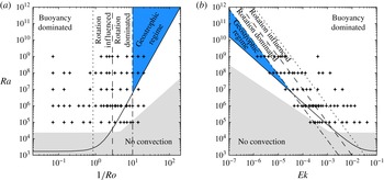
In the present DNS we can identify four different regimes with the proposed method. A summarising diagram with the proposed regime borders for
 $\mathit{Pr}=0.8$
and
 ${\it\Gamma}=1/2$
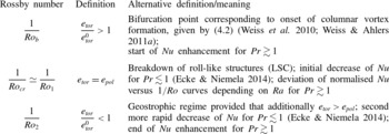
, i.e. the case primarily discussed here, is presented in figure 13. Naturally, the indicated borders may not be sharp and are susceptible to a change of the Prandtl number and the aspect ratio. Further, the characteristic inverse Rossby numbers defining these borders are given in table 2. Table 2 includes their definition based on the toroidal–poloidal energy decomposition and also alternative interpretations differing for fluids with
 $\mathit{Pr}\gtrsim 1$
and
 $\mathit{Pr}\lesssim 1$
.
Regime diagrams for rotating convection of a fluid with
 $\mathit{Pr}=0.8$
in a cylindrical cell with
 ${\it\Gamma}=1/2$
. The stars denote the DNS data presented here. The dark shaded area (blue online) indicates the geostrophic regime. The solid black line shows the prediction for the onset of convection by Chandrasekhar (Reference Chandrasekhar1961) for an infinite lateral extent. The grey shaded area corresponds to the range where there is indeed no convection for the
 ${\it\Gamma}=1/2$
cell considered here, based on the predictions by Buell & Catton (Reference Buell and Catton1983) and Herrmann & Busse (Reference Herrmann and Busse1993). (a) The dotted line corresponds to
 $1/\mathit{Ro}_{b}=0.86$
, the long-dashed line to
 $1/\mathit{Ro}_{cr}=1/\mathit{Ro}_{1}=2.86$
and dashed-dotted line to
 $1/\mathit{Ro}_{2}=10.0$
; see also table 2. (b) Similar to (a), but the rotation rate is expressed in terms of the Ekman number
 $\mathit{Ek}$
.

Definitions of the characteristic inverse Rossby numbers
 $1/\mathit{Ro}$
; always considered with respect to an increase of the rotation rate.

As long as
 $e_{tor}$
has the same value as in the non-rotating case, i.e.
 $e_{tor}/e_{tor}^{0}=1$
, the flow is completely dominated by buoyancy. As soon as the toroidal energy relative to the non-rotating case increases,
 $e_{tor}/e_{tor}^{0}>1$
, Rayleigh–Bénard convection is considered to be rotation influenced. This agrees well with the bifurcation point found by Weiss et al. (Reference Weiss, Stevens, Zhong, Clercx, Lohse and Ahlers2010) and Weiss & Ahlers (Reference Weiss and Ahlers2011a
), which gives
 $1/\mathit{Ro}_{b}=0.86$
for a cylindrical
 ${\it\Gamma}=0.5$
cell. At a rotation rate where the toroidal energy is greater than the poloidal one, convection is rotation dominated and large-scale roll structures, such as the LSC, are expected to cease to exist and instead columnar vortex structures dominate the flow. To reach this regime, however, the Rayleigh number has to be at least approximately
 $10^{7}$
. The critical inverse Rossby number is thus determined by the condition
 $e_{pol}=e_{tor}$
which gives
 $1/\mathit{Ro}_{cr}=1/\mathit{Ro}|_{e_{pol}=e_{tor}}\approx 3$
(
 $2.36\lesssim 1/\mathit{Ro}_{cr}\lesssim 3.33$
) for the cases considered. The transition determined in this way agrees very well with the one found by Ecke & Niemela (Reference Ecke and Niemela2014), who identify this point by a different scaling behaviour of
 $\mathit{Nu}$
, finding
 $1/\mathit{Ro}_{1}\approx 2.86$
. Ecke & Niemela (Reference Ecke and Niemela2014) also recognised a second transition where the scaling of
 $\mathit{Nu}$
changes once more at
 $1/\mathit{Ro}_{2}\approx 10.0$
. They argue that this can be related to the transition to the geostrophic regime. This Rossby number corresponds to the point at which the toroidal energy drops below the value for the non-rotating case,
 $e_{tor}/e_{tor}^{0}<1$
provided that
 $e_{tor}>e_{pol}$
. As can also be seen in figure 13, the lower bound for this regime would be given by the theoretical prediction by Chandrasekhar (Reference Chandrasekhar1961) for the onset of convection. Even though there is convection below this line because of the destabilising effect of the lateral wall, this form of convection is characterised by travelling-wave wall states.
An even better collapse of data for the Nusselt number and the toroidal and poloidal energy for all
 $\mathit{Ra}$
considered can be obtained by using
 $\mathit{Ra}\mathit{Ek}^{7/4}$
instead of
 $1/\mathit{Ro}$
as scaling variable, yielding
 $1.0\lesssim \mathit{Ra}\mathit{Ek}_{cr}^{7/4}\lesssim 2.0$
for the critical rotation rate where
 $e_{pol}\approx e_{tor}$
.
As a further example we also studied a fluid with
 $\mathit{Pr}=4.38$
in a
 ${\it\Gamma}=1$
cell. We again identified four different regimes and showed that they can be directly linked to the conventional criteria used for fluids with
 $\mathit{Pr}\gtrsim 1$
.
Hence, this method to classify regimes in rotating Rayleigh–Bénard convection based on velocity potentials is expected to work independently of the aspect ratio and of the Prandtl number.
Acknowledgements
S.H. wishes to thank K. Weinman and K. Petschel for helpful discussions about the numerical solution of Poisson equations and the interpretation of toroidal/poloidal energies, respectively. The authors are grateful to their referees for very constructive comments and suggestions. Further, the authors would like to express gratitude to the editor, E. Bodenschatz, S. Dreizler, G. Lube and D. Schleicher. The authors acknowledge financial support by the Deutsche Forschungsgemeinschaft (DFG) in the framework of SFB 963/1, project A6, and Heisenberg fellowship SH405/4 and also thank the Leibniz–Rechenzentrum (LRZ) in Garching for providing computational resources on SuperMUC.