1. Introduction
Combustion or thermoacoustic instability is the occurrence of large amplitude pressure oscillations in combustion chambers of rockets (Culick Reference Culick2006), aero and land-based gas turbine engines (Lieuwen & Yang Reference Lieuwen and Yang2005). It leads to catastrophic and premature engine damage. Catastrophic damage usually occurs in rockets. For example, the Apollo F-1 liquid rocket engine encountered an amplitude of more than 70 % of the mean combustion chamber pressure
 ${\sim}70\,{\textrm{bar}}$
, leading to immediate damage due to excessive fatigue load and heat transfer to the structure (Oefelein & Yang Reference Oefelein and Yang1993). However, gas turbine engine combustors, though, experiencing lower amplitudes
 ${\sim}20\,\%$
of mean pressure
 ${\sim}30\,{\textrm{bar}}$
, can still contribute to sustained fatigue loads to downstream components such as the turbine blades (Lieuwen Reference Lieuwen2002). A gradual deterioration leading to premature damage arises.
A positive feedback coupling between the combustion chamber acoustic field and flame leads to thermoacoustic instability. Despite significant progress in its prediction (Han, Li & Morgans Reference Han, Li and Morgans2015), control (Mcmanus, Poinsot & Candel Reference Mcmanus, Poinsot and Candel1993; Poinsot Reference Poinsot2017) and prognosis (Nair & Sujith Reference Nair and Sujith2014), tackling thermoacoustic instability is still a challenging problem. The challenge is posed due to the coupled actions of acoustic, hydrodynamic modes, turbulent flow, and upstream and downstream acoustic impedances in real engines (Poinsot Reference Poinsot2017). Their coupling is not fully understood.
In this large arena, our paper addresses one of the challenges of acoustic and hydrodynamic mode coupling in turbulent flow. Specifically, we focus on the phenomenon of vortex–acoustic lock-in. Modern combustors, afterburners, scramjets, etc., employ swirlers, bluff bodies or their combinations to anchor the flame (Zukoski & Oates Reference Zukoski and Oates1985; Mathur et al. Reference Mathur, Lin, Kennedy, Gruber, Donbar, Jackson and Billig2000; Bagheri, Hosseini & Wahid Reference Bagheri, Hosseini and Wahid2014). Vortex shedding occurs in such systems and disturbs the flame (Schadow & Gutmark Reference Schadow and Gutmark1992), which is a potent source of acoustic waves. The acoustic field of the combustion chamber, in turn, affects the vortex shedding, completing the formation of a coupled system. Both phenomena possess characteristic frequencies. Two important observations are made during lock-in. (i) The coupled system oscillates at a common frequency over a range of flow parameters. The common frequency can be close to the vortex shedding (Chakravarthy, Sivakumar & Shreenivasan Reference Chakravarthy, Sivakumar and Shreenivasan2007) or the acoustic frequency (Poinsot et al. Reference Poinsot, Trouve, Veynante, Candel and Esposito1987). (ii) Lock-in is observed both during large amplitude combustion instability (Poinsot et al. Reference Poinsot, Trouve, Veynante, Candel and Esposito1987) and its suppression (Emerson & Lieuwen Reference Emerson and Lieuwen2015). Our previous experiments (Singh & Mariappan Reference Singh and Mariappan2021) and theoretical analysis (Britto & Mariappan Reference Britto and Mariappan2023) show the above-mentioned two features.
One encounters the background stochastic turbulent fluctuations while understanding the lock-in in practical combustors. Such stochastic environments lead to: (i) masking the underlying or creating new dynamical features (Waugh & Juniper Reference Waugh and Juniper2011b ; Jegadeesan & Sujith Reference Jegadeesan and Sujith2013; Faure-Beaulieu et al. Reference Faure-Beaulieu, Indlekofer, Dawson and Noiray2021) and (ii) creating non-trivial phenomena such as stochastic/coherence resonance (Kabiraj et al. Reference Kabiraj, Steinert, Saurabh and Paschereit2015; Li & Zhao Reference Li and Zhao2017; Guk, Seo & Lee Reference Guk, Seo and Lee2024). On the bright side, the stochastic fluctuations have information for: (i) system identification (Lee et al. Reference Lee, Kim, Gupta and Li2021) and (ii) prognosis of an impending instability (Sengupta, Rasmussen & Juniper Reference Sengupta, Rasmussen and Juniper2021).
Initial studies on system identification approximated the stochastic fluctuations by incorporating a Gaussian white noise term in the low-order model (for example, Noiray & Schuermans Reference Noiray and Schuermans2013). The resulting stochastic differential equations were converted to the corresponding Fokker–Planck equation for the probability of the pressure fluctuations (or any other measurable quantity). Experimentally measured probabilities are then fitted to identify the model parameters. Later, Bonciolini, Boujo & Noiray (Reference Bonciolini, Boujo and Noiray2017) showed that the above-mentioned procedure leads to incorrect system identification for large correlation time of the stochastic fluctuations. In real systems, turbulent fluctuations are coloured noise (Majda et al. Reference Majda, Timofeyev and Vanden Eijnden1999). Ornstein–Uhlenbeck (OU) noise was proposed to approximate the coloured noise. Furthermore, OU noise was shown to spectrally reproduce the combustion noise of turbulent flames (Bonciolini, Boujo & Noiray Reference Bonciolini, Boujo and Noiray2016). Recent papers use OU noise in their system identification (Lee et al. Reference Lee, Kim, Gupta and Li2021; Vishnoi et al. Reference Vishnoi, Gupta, Saurabh and Kabiraj2022).
Similar to system identification, various measures, such as the Hurst exponent (Nair & Sujith Reference Nair and Sujith2014), coherence factor (Kabiraj et al. Reference Kabiraj, Steinert, Saurabh and Paschereit2015; Guk et al. Reference Guk, Seo and Lee2024) and machine learning methods (Kobayashi et al. Reference Kobayashi, Murayama, Hachijo and Gotoda2019; Sengupta et al. Reference Sengupta, Rasmussen and Juniper2021; Lyu, Fang & Wang Reference Lyu, Fang and Wang2023) for instability prognosis (early warning indicators), strongly depend on the underlying noise type. A recent paper (Vishnoi & Kabiraj Reference Vishnoi and Kabiraj2024) systematically re-emphasised the strong effect of noise correlation type on the performance of the early warning indicators.
Overall, the noise type (correlation time, power-spectrum distribution, etc.) strongly affects the basic understanding, system identification and prognosis of combustion instability. Therefore, performing a theoretical analysis of vortex–acoustic lock-in with stochastic fluctuations having non-zero correlation times is vital. In our previous investigation (Mariappan Reference Mariappan2022), we studied the effects of an additive Gaussian white noise on vortex–acoustic lock-in in the parlance of combustion instability. The added noise was assumed to represent the effects of turbulence in the combustor. The major conclusions of the paper are the following. (i) The addition of noise reduces the extent of lock-in. (ii) Lock-in can lead to the occurrence of both instability and amplitude suppression. (iii) Of the various orders of stochastic lock-in (shortened as s-lock-in), 1 : 1 lock-in serves as the most favourable condition for instability. (iv) Stochastic resonance (SR) is too weak to be the leading cause of instability. A proposition for its weakness is as follows. SR is measured by a quantity signal-to-noise ratio (SNR). SNR is defined as the ratio of spectral powers in the system response (vortex shedding circulation, refer to Mariappan Reference Mariappan2022) to the noise at the forcing frequency. The maximum SNR is approximately 1.6. Other similar noise-induced phenomena, such as coherence resonance, have SNR (based on coherence factor) above 4.0 (Kabiraj et al. Reference Kabiraj, Steinert, Saurabh and Paschereit2015).
2. Motivation
In practical combustors, the turbulent fluctuations are coloured and multiplicative (Majda et al. Reference Majda, Timofeyev and Vanden Eijnden1999; Gottwald & Harlim Reference Gottwald and Harlim2013). Therefore, it is imperative to re-perform the investigation of Mariappan (Reference Mariappan2022), with a multiplicative noise generated by an OU process. It forms the motivation of the paper. Multiplicative noise changes the location and stability of the fixed points (Graham & Schenzle Reference Graham and Schenzle1982). It leads to non-trivial behaviour, such as stochastic lock-in (Löcher et al. Reference Löcher, Cigna and Hunt1998) and resonance (Zaikin & Schimansky-Geier Reference Zaikin and Schimansky-Geier1998). The book by Anishchenko et al. (Reference Anishchenko, Astakhov, Neiman, Vadivasova and Schimansky-Geier2007) provides a good reference for studying noise-induced phenomena in dynamical systems. The OU process is a surrogate for the coloured noise. Previous studies (Bonciolini et al. Reference Bonciolini, Faure-Beaulieu, Bourquard and Noiray2021; Vishnoi & Kabiraj Reference Vishnoi and Kabiraj2024) indicate that such a surrogate models the statistics of pressure oscillations in a turbulent combustor.
The rest of the paper is arranged as follows. Section 3 describes the model formulation and its rationale. We then briefly discuss the solution procedure in § 4. The model parameter range relevant to the lab and industry scale combustors is identified in § 5. The simulation results and their interpretations in relation to combustion instability are presented in §§ 6–8. Finally, § 11 briefs on the salient conclusions from the paper.
3. Formulation and governing equations
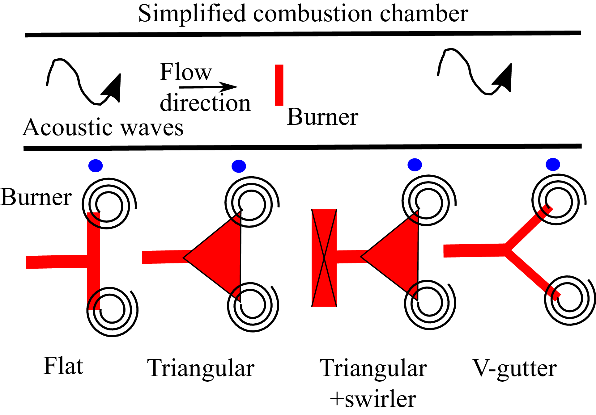
Figure 1 represents a combustion chamber schematic, where the flame is anchored by a bluff body or combined with other means (for example, swirler). Vortices are shed from the sharp corners of the bluff body. Although they are shed alternatively between the top and bottom ends, only their shedding locations are represented graphically (spirals).
Top of the figure shows a schematic of a sector combustion chamber, where a bluff body anchors the flame. The red line represents the bluff body burner containing the flame. Acoustic waves perturb the flame and vice versa, leading to the thermoacoustic feedback. The lower part of the figure indicates some commonly used bluff body burners for flame anchoring. Vortices (represented as spirals) are shed from the sharp corners of the bluff body. Blue dots indicate the reference location for the instantaneous velocity
 $1+u$
. The location is outside the boundary layer.

The vortex shedding process is described by the well-established and amply used low-order of Matveev & Culick (Reference Matveev and Culick2003) to study combustion instability (for example, Pawar et al. Reference Pawar, Seshadri, Unni and Sujith2017, Boulal et al. Reference Boulal, Genot, Klein, Fabignon, Vincent-Randonnier and Sabelnikov2023). The model originates from the numerical computations performed to capture vortex shedding (Clements Reference Clements1973). Although the model appears to be phenomenological, it is quantitatively accurate with the experiments of Fage & Johansen (Reference Fage and Johansen1927) in predicting: (i) the temporal accumulation of circulation
 $\varGamma$
at the sharp corner and (ii) the shedding frequency for a hydrodynamic system.
The model applies to flow over two-dimensional bluff body geometries (figure 1). It may not yield good results when applied to practical swirl-stabilised combustors, where vortex shedding occurs from multiple locations and contains three-dimensional effects. Despite the model limitations, it reproduced fairly well the: (i) uni-directionally forced lock-in boundary (Britto & Mariappan Reference Britto and Mariappan2019) observed in hydrodynamically self-excited flames (Li & Juniper Reference Li and Juniper2013) and (ii) spectral distribution of bi-directionally coupled thermoacoustic oscillation (Britto & Mariappan Reference Britto and Mariappan2023) in a vortex shedding combustor. Moreover, the stochastic version of the model coupled with combustor acoustic field equations captures the intermittent thermoacoustic oscillations of the experiments (Nair & Sujith Reference Nair and Sujith2015). All the experiments have three-dimensional effects. Therefore, we believe that the model predictions are reasonably accurate, perhaps quantitatively.
The total circulation near the sharp corner
 $\varGamma$
evolves according to the following equation. Here,
 $\xi (t)$
is the stochastic noise added in this paper (to be discussed shortly). The Matveev & Culick (Reference Matveev and Culick2003) model is purely deterministic. The equations are non-dimensionalised (refer to Britto & Mariappan Reference Britto and Mariappan2019 for details).
 \begin{align} &\frac {{\textrm{d}}\varGamma }{{\textrm{d}}t}=\frac {\left [1+u(t)\right ]^2}{2}+ \xi (t),\quad u(t)=A\sin (\omega t+\phi _0),\quad \omega =2\pi f, \end{align}
 \begin{align} &\frac {{\textrm{d}}\xi }{{\textrm{d}}t}=-\frac {\xi }{\epsilon _n}+\frac {A_n}{\sqrt {\epsilon _n/2}}\eta (t),\quad A^2_n=A^2_{n0}(1+\zeta \varGamma ^2), \end{align}
 \begin{align} &\varGamma _{\textit{sep}}=\frac {1+u(t)}{2}, \end{align}
 \begin{align} &\varGamma (t=t_{m-1})=0\quad \textrm {Initial condition}, \end{align}
 \begin{align} &t_m=\inf \left [t\gt t_{m-1}:\varGamma (t)=\varGamma _{\textit{sep}}(t)\right ]\quad \textrm {Reset condition}, \end{align}
where
 $\inf$
stands for the greatest lower bound of the set. Time instants
 $t_{m-1}$
and
 $t_m$
correspond to
 $(m-1)$
th and
 $m$
th vortex shedding, respectively. Here,
 $\varGamma$
begins from zero at the end of the
 $(m-1)$
th shedding (3.4). It evolves stochastically according to (3.1), until it reaches a critical value,
 $\varGamma =\varGamma _{\textit{sep}}$
. The
 $m$
th vortex is shed at
 $t_m$
(3.5).
The instantaneous velocity along the separation edge outside the boundary layer (marked as blue dots in figure 1),
 $1+u$
(1 and
 $u$
represent steady-state and fluctuating velocity, respectively), serves as the source for
 $\varGamma$
. External harmonic velocity excitation,
 $u=A\sin (\omega t+\phi _0)$
, is imposed with
 $A$
,
 $\omega$
,
 $f$
and
 $\phi _0$
representing the amplitude, circular frequency, oscillation frequency and initial phase of the excitation, respectively. Here,
 $u$
acts as a surrogate for the acoustic field during combustion instability. The surrogate considerably simplifies the mathematical amenability, instead of operating with the fully coupled system in the presence of noise. It allows one to make a better physical interpretation of the simulation results.
An OU noise
 $\xi$
is added to the evolution equation of
 $\varGamma$
(3.1). Equation set (3.1)–(3.5) falls in the broad category of stochastic integrate-and-fire models. Accumulation of circulation
 $\varGamma$
, followed by the subsequent shedding, form the integrate and fire components, respectively. Apart from modelling vortex shedding, it is employed and studied in a wide variety of fields: biology (Plesser & Tanaka Reference Plesser and Tanaka1997; Tateno & Jimbo Reference Tateno and Jimbo2000), electronics (Goldberg, Cauwenberghs & Andreou Reference Goldberg, Cauwenberghs and Andreou2001), biophysics (Ramlow, Falcke & Lindner Reference Ramlow, Falcke and Lindner2023), etc.
As a side note, the factor 1/2 in the evolution of
 $\varGamma$
(3.1) is an assumption from the original model by Clements (Reference Clements1973). The numerical value is reasonably close to the experimental observation of Fage & Johansen (Reference Fage and Johansen1927). In the present work, the equation set (3.1)–(3.5) is non-dimensionalised, such that the natural (absence of external excitation
 $u=0$
and noise
 $\xi =0$
) vortex shedding period equals 1. The same 1/2 factor is incorporated in (3.3) for this purpose.
In principle,
 $\xi$
can be appended anywhere in the model. However, it is added to the evolution equation of circulation
 $\varGamma$
(3.1), in favour of other locations, such as to the acoustic velocity, threshold circulation
 $\varGamma _{\textit{ref}}$
(3.3) or their combinations. The first option of incorporating
 $\xi$
in the governing equation allows one to write a corresponding Fokker–Planck equation. To the best of the author’s knowledge, all the stochastic integrate-and-fire models used in various fields and employing the Fokker–Planck framework have chosen the above-mentioned option (for example, Plesser & Geisel Reference Plesser and Geisel1999 in biology, Goldberg et al. Reference Goldberg, Cauwenberghs and Andreou2001 in electronics). Experimental evidence in biology (Burkitt Reference Burkitt2006) does point to the above-mentioned choice. In general, a physical interpretation of the choice is unclear in other fields. In spite of the opacity, the above-mentioned model captures the firing (vortex shedding instances) statistics of the neurons observed in biological experiments (Burkitt Reference Burkitt2006). For fluid flow systems, Zare, Jovanović & Georgiou (Reference Zare, Jovanović and Georgiou2017) have shown that adding a noise term in the governing equation (Navier–Stokes equation in their case) captures the second-order turbulence statistics. It is still unclear whether the same approach would work for the present low-order stochastic integrate-and-fire model. At this point, we believe a similar conclusion to that in biological neurons is expected for the choice of the model for the current system, rather than a rigorous physical explanation.
The OU noise variable,
 $\xi$
, follows (3.2), with
 $\eta (t)$
representing a Gaussian white noise of unit amplitude. The
 $\xi$
provides a coloured noise of amplitude
 $A_n$
. Additionally,
 $\xi$
is exponentially auto-correlated,
 $\langle \xi (t)\xi (t^{\prime})\rangle =A_n^2 \exp (-|t-t^{\prime}|/\epsilon _n)$
(
 $\langle \,\rangle$
indicating the ensemble average), where
 $\epsilon _n$
is the correlation time. The subscript
 $n$
represents noise parameters. Note that the coefficient of
 $\eta (t)$
in (3.2) can either be chosen as
 $A_n/\sqrt {\epsilon _n/2}$
(for example, Middleton et al. Reference Middleton, Chacron, Lindner and Longtin2003) or
 $\eta (t)/\epsilon _n$
(for example, Bonciolini et al. Reference Bonciolini, Faure-Beaulieu, Bourquard and Noiray2021; Vishnoi et al. Reference Vishnoi, Gupta, Saurabh and Kabiraj2022). Choosing the former renders the amplitude of the coloured noise
 $\xi (t)$
to be
 $A_n$
irrespective of the value of
 $\epsilon _n$
. However, preference for the latter leaves the noise amplitude
 $A_n/\sqrt {\epsilon _n}$
: a quantity varying with
 $\epsilon _n$
. We prefer the former case in this paper, as one can vary
 $A_n$
and
 $\epsilon _n$
independently without requiring adjustments in the effective noise amplitude. The downside of our approach is that the correlation
 $\langle \xi (t)\xi (t^{\prime})\rangle \rightarrow A_n^2 \epsilon _n \delta (|t-t^{\prime}|)$
as
 $\epsilon _n \rightarrow 0$
(
 $\delta (x)$
is the Dirac-delta function). The correlation contains the
 $\epsilon _n$
term and, therefore,
 $\xi$
does not represent strictly a Gaussian noise in the limit of
 $\epsilon _n\rightarrow 0$
. However, for non-zero
 $\epsilon _n$
, the correlation time of
 $\xi$
does drop. Since the present paper discusses the variation with non-zero
 $\epsilon _n$
considering the lab-scale and practical combustors (§ 5), we believe that the above-mentioned functional choice for the coefficient of
 $\eta (t)$
is appropriate.
To incorporate multiplicative noise,
 $A_n$
is made a function of
 $\varGamma$
. The rationale for the functional form of
 $A_n$
is discussed as follows. Turbulence causes non-Gaussian probability density functions (p.d.f.s) of vorticity (Wilczek, Daitche & Friedrich Reference Wilczek, Daitche and Friedrich2011). The diffusion term in the corresponding Fokker–Planck equation, governing the evolution of vorticity p.d.f., shows a strong dependence on vorticity (multiplicative noise). Numerical simulations by Wilczek & Friedrich (Reference Wilczek and Friedrich2009) indicate that the dependence is quadratic in vorticity. Motivated by the above-mentioned simulations, we choose the diffusion term in (4.7) as
 $(A_n/A_{n0})^2=1+\zeta \varGamma ^2$
, where
 $\zeta$
is the coefficient defining the strength. Both
 $A_{n0}$
and
 $\zeta$
are constants.
4. Solution procedure
The solution procedure for (3.1)–(3.5) is as follows. Considering the arguments of Mariappan (Reference Mariappan2022), it is convenient to replace
 $t$
by elapsed time
 $t^{\prime}$
, the time passed since the shedding of the previous vortex. In this way, (3.1)–(3.5) are solved for the shedding time period
 $\tau _m=t_m-t_{m-1}$
and phase
 $\phi _m=(\omega \tau _m + \phi _{m-1})\,{\textrm{modulo}}\,2\pi$
for the
 $m$
th vortex. Later, the Fokker–Planck equation (4.1) requires knowledge of the phase of the previous vortex shedding
 $\phi _{m-1}$
(4.6) to calculate the probability of the current (
 $m$
th) shedding time period (the subscript
 $m-1$
is dropped). Equation set (4.1)–(4.6) is solved for discrete (100 in the present paper) values of
 $0\leqslant \phi \lt 2\pi$
to obtain the shedding period probability. Since the current shedding (
 $m$
th vortex) period
 $\tau _m$
depends on the previous (
 $m-1$
th vortex) shedding phase, the shedding process is Markovian and non-stationary. Detailed discussion on the requirement to use
 $\phi _m$
space is made in § 2.1 of our previous work (Mariappan Reference Mariappan2022). The non-stationarity is a characteristic feature of integrate-and-fire models.
Since the process is Markovian, the vortex-shedding events form a connected series of spike trains (spikes occurring at
 $t_m$
s). The long-term statistics (as
 $t\rightarrow \infty$
) of the train provide information about the stochastic shedding process. It can then be used to determine stochastic lock-in and resonance. The statistics are obtained in two steps (details from Mariappan Reference Mariappan2022).
-
(i) Determination of the conditional probability distribution
 $\rho (\tau |\phi )$
of vortex shedding time period
$\tau$
, given the shedding phase
$\phi$
at the end of the previous shedding.
-
(ii) Assembly of the vortex shedding events to obtain the stationary (
$t,\,m\rightarrow \infty$
) probability distribution for shedding time period
$\rho _s$
and phase
$\phi _s$
(subscript
$s$
indicates stationary variables)


The Fokker–Planck equation to be solved in the first step differs from that of Mariappan (Reference Mariappan2022), owing to the presence of OU multiplicative noise. However, the solution procedure associated with the second step remains the same.
4.1. Step 1: Determination of conditional probability vortex shedding time period
The evolution of the joint probability density function,
 ${\mathscr{f}}$
, for
 $\varGamma$
and
 $\xi$
in the elapsed time
 $t^{\prime}$
is given by the following Fokker–Planck equation (corresponding to (3.1)–(3.5)):
 \begin{align} \frac {\partial {\mathscr{f}}}{\partial t^{\prime}}+\left (\frac {(1+u)^2}{2}+\xi \right ) \frac {\partial {\mathscr{f}}} {\partial \varGamma }&=\frac {1}{\epsilon _n}\frac {\partial \left (\xi {\mathscr{f}}\right )} {\partial \xi }+\frac {1}{\epsilon _n} \frac {\partial ^2 \left (A_n^2 {\mathscr{f}}\right )} {\partial \xi ^2}, \end{align}
 \begin{align} {\mathscr{f}}(\varGamma ,\xi ,t^{\prime}=0)&=\delta (\varGamma )\frac {e^{-\left ({\xi }^2/2{A_{n0}^2}\right )}}{\sqrt {2\pi } A_{n0}}\quad \textrm {initial condition}, \end{align}
 \begin{align} {\mathscr{f}}(\varGamma =\varGamma _{\textit{sep}},\xi ,t^{\prime})&=0\quad \textrm {boundary condition}, \end{align}
 \begin{align} {\mathscr{f}}(\varGamma \rightarrow -\infty ,\xi ,t^{\prime})&=0\quad \textrm {boundary condition}, \end{align}
 \begin{align} {\mathscr{f}}(\varGamma ,\xi \rightarrow \pm \infty ,t^{\prime})&=0\quad \textrm {boundary condition}, \end{align}
 \begin{align} \varGamma _{\textit{sep}}=\frac {1+u(t^{\prime})}{2}&=\frac {1+A\sin (\omega t^{\prime}+\phi )}{2}. \\[9pt] \nonumber \end{align}
The joint probability
 ${\mathscr{f}}(\varGamma ,\xi ,t^{\prime})$
is read as the probability that the vortex circulation and noise takes a value between
 $\varGamma \,\&\, {\textrm{d}}\varGamma$
and
 $\xi \,\&\, \xi +{\textrm{d}}\xi$
, respectively at a time
 $t^{\prime}$
, given its initial distribution at time
 $t^{\prime}=0$
. The above-mentioned Fokker–Planck equation is first order in
 $t^{\prime},\,\varGamma$
and second order in
 $\xi$
, requiring one initial, one boundary and two boundary conditions in
 $t^{\prime},\,\varGamma$
and
 $\xi$
, respectively. Here,
 $\varGamma$
takes a deterministic value of zero at the end of an
 $(m-1)$
th vortex shedding event. Therefore, the dependence of
 ${\mathscr{f}}$
on
 $\varGamma$
at
 $t^{\prime}=0$
is a Dirac-delta function placed at the origin,
 $\delta (\varGamma )$
.
At this point, one can choose various functional dependencies of
 ${\mathscr{f}}$
on
 $\xi$
at
 $t^{\prime}=0$
. Since the present investigation requires the stationary statistics of the shedding events, we choose the stationary probability distribution of
 $\xi$
as the initial condition for
 ${\mathscr{f}}$
. The stationary p.d.f. is Gaussian:
 ${e^{-({\xi }/{2A_{n0}})^2}}/{\sqrt {2\pi } A_{n0}}$
(zero mean and standard deviation
 $A_{n0}$
). A similar choice is made by Palleschi & De Rosa (Reference Palleschi and De Rosa1992).
For
 $t^{\prime}\gt 0$
, the circulation of the
 $m$
th vortex increases according to (3.1)–(3.2). It increases until
 $\varGamma =\varGamma _{\textit{sep}}$
, leading to the
 $m$
th shedding. Since
 $\varGamma$
is reset to zero immediately after the
 $m$
th shedding, the corresponding probability,
 ${\mathscr{f}}(\varGamma =\varGamma _{\textit{sep}},\xi ,t^{\prime})=0$
(4.3). Boundary conditions (4.4)–(4.5) emphasise that
 ${\mathscr{f}}$
vanishes at
 $\pm \infty$
in the
 $\varGamma ,\,\xi$
domain, as appropriate.
The boundary condition (4.3) is time-varying due to
 $\varGamma _{\textit{sep}}$
, which poses difficulty in the numerical solution procedure. Since the initial dependence of
 ${\mathscr{f}}$
is Gaussian (4.2), it is possible to obtain a series solution in terms of Hermite polynomials (similar to Frisch & Nowakowski Reference Frisch and Nowakowski1993). The above-mentioned two points prompt us to perform a change of independent variables as follows:
 $\hat t=t,\ \hat \varGamma =1-{\varGamma }/{\varGamma _{\textit{sep}}},\ \hat \xi = {\xi }/A_{n0}$
. The transformation renders (4.1)–(4.5) to become the following:
 \begin{align} \frac {\partial {\mathscr{f}}}{\partial \hat t}+\left (\frac {(1-\hat \varGamma )\,{\textrm{d}}u/{\textrm{d}}\hat t-(1+u)^2}{1+u}-\frac {2A_{n0}\hat \xi }{(1+u)} \right ) \frac {\partial {\mathscr{f}}} {\partial \hat \varGamma }&=\frac {1}{\epsilon _n}\frac {\partial \big(\hat \xi {\mathscr{f}}\big)} {\partial \hat \xi }+\frac {1}{\epsilon _n}\left (\frac {A_n}{A_{n0}}\right )^2\frac {\partial ^2 {\mathscr{f}} } {\partial \hat \xi ^2}, \end{align}
 \begin{align} {\mathscr{f}}(\hat \varGamma ,\hat \xi ,\hat t=0)=\delta (\hat \varGamma -1)\frac {e^{-\big (\hat \xi ^2/2\big )}}{|1+A\sin \phi |\sqrt {\pi /2} A_{n0}}&\quad \textrm {initial condition}, \end{align}
 \begin{align} {\mathscr{f}}(\hat \varGamma =0,\hat \xi ,\hat t)=0&\quad \textrm {boundary condition}, \end{align}
 \begin{align} {\mathscr{f}}(\hat \varGamma \rightarrow \infty ,\hat \xi ,\hat t)=0&\quad \textrm {boundary condition}, \end{align}
 \begin{align} {\mathscr{f}}(\hat \varGamma ,\hat \xi \rightarrow \pm \infty ,\hat t)=0&\quad \textrm {boundary condition}. \\[9pt] \nonumber \end{align}
We use Galerkin method to solve (4.7). Orthonormal Hermite functions
 $(\varphi _p,\,\psi _p$
of
 $p$
th degree) in both
 $\hat \varGamma$
and
 $\hat \xi$
are used as basis functions. They satisfy the boundary conditions, (4.9)–(4.11). The solution is expanded in the following form:
 \begin{align} {\mathscr{f}}\big (\hat \varGamma , \hat \xi , \hat t \big )=\sum _{\substack {r=0,1,2,\ldots R\\p=1,3,5,\ldots P}}a_{rp}\left (t\right )\varphi _r\big (\hat \xi \big ) \psi _p\big (\hat \varGamma \big ), \quad t\geqslant 0,-\infty \lt \hat \xi \lt \infty ,\,0\leqslant \hat \varGamma \lt \infty, \end{align}
where
 $\varphi _p (\hat \xi )=H_p (\hat \xi )e^{-\hat \xi ^2/2}/\sqrt { (\sqrt \pi 2^pp!) )},\,\psi _p (\hat \varGamma )=H_p (\hat \varGamma )e^{-\hat \varGamma ^2/2}/\sqrt { (\sqrt \pi 2^{p-1}p!) )}$
, with
 $\int _{-\infty }^{\infty }\varphi _r(x) \varphi _s(x)\,{\textrm{d}}x=\delta ^k_{rs},\,\int _{0}^{\infty }\psi _p(x) \psi _q(x)\,{\textrm{d}}x=\delta ^k_{pq}$
. Here,
 $\delta ^k_{rs}$
is the Kronecker-delta function (superscript
 $k$
is to differentiate the symbol from the Dirac-delta function used earlier). Additionally,
 $H_r$
is the
 $r$
th degree physicist’s Hermite polynomials. The Galerkin expansion satisfies the boundary conditions (4.9)–(4.11). Here,
 $R,\,P$
indicate the total number of Galerkin modes. Applying Galerkin projection on (4.7)–(4.8), we obtain a first-order ordinary differential equation for the time evolution of
 $a_{sq}$
, along with its initial condition,
 \begin{align} \frac {{\textrm{d}} a_{sq}}{{\textrm{d}}\hat t} \!=\! \sum _{\substack {r,p\\}}a_{rp} \! \left [\! I^{\alpha }\frac {\left (1+u\right )^2-{\textrm{d}}u/{\textrm{d}}\hat t}{1+u}+I^{\beta }\frac {{\textrm{d}}u/{\textrm{d}}\hat t}{1+u}+I^{\gamma }\frac {2A_{n0}}{(1+u)}+\frac {I^{\delta }+\zeta (1+u)^2I^{\varUpsilon }/4}{\epsilon _n}\! \right ]\!, \\[-28pt] \nonumber \end{align}
 \begin{align} a_{sq}(\hat t=0)=\frac {\sqrt {2}H_q(1)e^{-1/2}\delta ^k_{s0}}{|1+A\sin \phi |A_{n0}\pi 2^{s+q-1}s!q!} ,\end{align}
where
 $I^{\alpha },\,I^{\beta },\ldots, I^{\varUpsilon }$
are the Galerkin integrals, which are functions of the Hermite functions of degrees
 $p,q,r,s$
. Their functional forms are given in Appendix A. They are evaluated a priori to the simulations.
Equation (4.13) is time-marched to obtain the joint probability
 ${\mathscr{f}}$
. The conditional probability
 ${\mathscr{p}}$
for the circulation is then evaluated as
 ${\mathscr{p}}(\varGamma ,t)=\int _{\xi =-\infty }^{\infty }{\mathscr{f}}\,{\textrm{d}}\xi$
. Determination of the conditional probability of vortex shedding time period
 $\rho (\tau /\phi )$
is posed as a first passage time problem, when
 $\varGamma$
reaches
 $\varGamma _{\textit{sep}}$
for the first time. An expression is as follows:
 $\rho (\tau /\phi )=- (\textrm{d}/{{\textrm{d}}t})(\int _{-\infty }^{\varGamma _{\textit{sep}}(t)}{\mathscr{p}}\, {\textrm{d}}\varGamma )_{t=\tau }$
(details from Mariappan Reference Mariappan2022). After applying the coordinate transformation and Galerkin ansatz, the following expression for
 $\rho$
is obtained in terms of the Galerkin coefficients:
 \begin{equation} \rho (\tau /\phi )=-\frac {A_{n0}}{2}\sum _{\substack {r,p}}\left [(1+u)\frac {{\textrm{d}}a_{rp}}{{\textrm{d}}t}+\frac {{\textrm{d}}u}{{\textrm{d}}t}a_{rp}\right ]I^{\nu }_rI^{\varsigma }_p .\end{equation}
The dependence on
 $\phi$
occurs through the initial condition (4.8). In the next step, we assemble the shedding events to obtain a spike train and its corresponding long-time statistics.
4.2. Step 2: Assembly of vortex shedding events and identification of stochastic lock-in
The conditional probability
 $(\rho )$
of the
 $m$
th vortex shedding time is determined solely by the
 $m-1$
th shedding phase
 $\phi$
. Therefore, given a probability distribution
 $(\chi^{\boldsymbol{0}})$
of the first vortex shedding phase, one can evolve the probability distribution of the subsequent shedding phases
 $( \chi^{\boldsymbol{1}},\,\chi ^{\boldsymbol{2}},\,\chi^{\boldsymbol{3}},\ldots )$
. The successive probability distributions are related by
 $\chi^{\boldsymbol{m+1}} = \boldsymbol{T}\chi ^{\boldsymbol{m}}$
, where
 $\boldsymbol{T}$
is the transition probability matrix. The matrix acts as a dynamical operator, which transitions the shedding phase probability distribution from one (
 $m$
th) to the next (
 $m+1$
th), shedding instance. An expression of the matrix requires the introduction of additional variables. Therefore, readers are directed to refer to § 2.2 of Mariappan (Reference Mariappan2022). In long time
 $t\rightarrow \infty$
, the shedding phase probability,
 $\chi ^{\boldsymbol{s}}=\chi ^{\boldsymbol{m\rightarrow \infty}}$
, reaches a stationary distribution,
 $\chi^{\boldsymbol{s}}$
. Here,
 $\chi^{\boldsymbol{s}}$
is the first eigenvector of
 $\boldsymbol{T}$
, having an eigenvalue of 1 (Plesser & Geisel Reference Plesser and Geisel1999). The corresponding probability of the stationary vortex shedding time period,
 $\rho _s(\tau )=\int _0^{2\pi }\rho (\tau /\phi )\,{\textrm{d}}\phi$
, is calculated. The second and subsequent eigenvalues of
 $\boldsymbol{T}$
decide the route taken by the system on its way to
 $\chi^{\boldsymbol{s}}$
. Their qualitative change from complex to real values determines the onset of stochastic lock-in (s-lock-in). We restrict ourselves to 1 : 1 s-lock-in in this paper as our previous investigation (Mariappan Reference Mariappan2022) indicated that it favours combustion instability. Therefore, the region of the phase of the second eigenvalue equal to zero indicates the s-lock-in (Tateno & Jimbo Reference Tateno and Jimbo2000).
Having discussed the solution procedure, the next step would be to identify the parameters and their numerical ranges, which are of interest to academic and industrial combustor configurations. There are five parameters in the model (3.1)–(3.2): (i) amplitude
 $A$
; (ii) frequency
 $f$
of the harmonic excitation; (iii) amplitude
 $A_{n0}$
; (iv) correlation time
 $\epsilon _n$
and (v) multiplicative noise factor
 $\zeta$
of the OU noise. Their ranges are determined in the following section.
5. Identification of noise parameters
Extensive experimental results (Shivashankara, Strahle & Handley Reference Shivashankara, Strahle and Handley1973; Rajaram & Lieuwen Reference Rajaram and Lieuwen2009) indicate that (direct) combustion noise (acoustic pressure fluctuations) due to radiation from a turbulent flame: (i) is broadband and (ii) contains a non-monotonic distribution of spectral power, with a peak occurring at a certain frequency
 $\varpi _{peak}$
. The underlying flame heat release rate fluctuations
 $Q$
have a power spectral density (PSD), which is almost flat at low frequencies until
 $\varpi _{peak}$
, followed by a power law decay with an exponent in the range
 $(-2.1,-3.2)$
(Rajaram & Lieuwen Reference Rajaram and Lieuwen2009). Compared with the above-mentioned features, we observe the following with the input noise from the OU process
 $\xi$
. The PSD of
 $\xi$
generated by the OU process, at a frequency
 $\varpi$
, equals
 $A_{n0}^2\epsilon _n/2\pi (1+(2\pi \varpi \epsilon _n)^2)$
(in the absence of multiplicative noise
 $\zeta =0$
). Therefore, the PSD of
 $\xi$
stays flat at low frequencies until
 $\varpi \approx 1/\epsilon _n$
. It follows a power-law decay: PSD of
 $\xi \sim \varpi ^{-2}$
for large
 $\varpi$
. The spectral behaviour of
 $\xi$
is qualitatively the same as that of
 $Q$
, and the power law decay exponent is also close to the range observed from the experiments. Therefore, imitating the heat release rate of combustion noise by the OU process is a good approximation, at least in the spectral domain.
In the temporal domain, intermittent oscillations (quiet zones with bursts of large amplitudes) are observed in thermoacoustic interactions (for example, Nair & Suijith Reference Nair and Suijith2013; Bonciolini et al. Reference Bonciolini, Faure-Beaulieu, Bourquard and Noiray2021). However, the Fokker–Planck framework describes the evolution of the p.d.f. rather than time series, and intermittent oscillations appear to be missed in the analysis. However, temporal and p.d.f. domain analysis by Reuther & Kähler (Reference Reuther and Kähler2020) in a turbulent boundary layer does indicate that intermittency is captured by the non-Gaussian nature in the p.d.f. We do observe a similar feature (figure 2 b,c and figure 3 b,c,e,f). Therefore, the Fokker–Planck framework does capture intermittency, albeit indirectly.
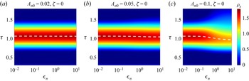
Variation of p.d.f. of shedding time period,
 $\rho _s$
with the correlation time
 $\epsilon _n$
for additive (
 $\zeta =0$
) noise at various noise amplitudes (
 $A_{n0}=0.02,\,0.05,\,0.1$
) in the absence of harmonic excitation. The dashed white curve represents the mode of
 $\rho _s$
distribution.

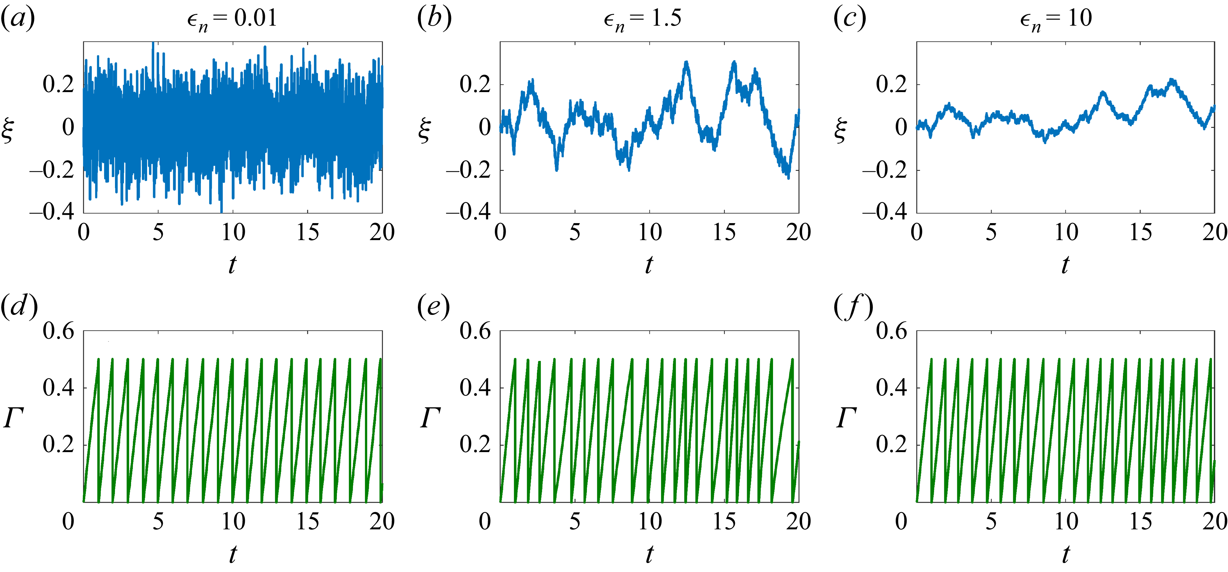
Time domain simulations of (a–
c)
 $\xi$
, (d–f)
 $\varGamma$
at three increasing
 $\epsilon _n=0.01,\,1.5,\,10$
.
 $A_{n0}=0.1, \zeta =0$
is used for all the simulations. The same initial condition
 $\xi _0=0$
and seed for
 $\eta _s$
are used for illustration purposes.

The Matveev & Culick (Reference Matveev and Culick2003) model suggests that the heat release rate transported by the vortex is proportional to its circulation
 $\varGamma$
. Therefore,
 $\xi$
is added to the evolution of
 $\varGamma$
in (3.1) of this paper to model the effect of heat release rate fluctuations due to combustion noise. A similar approach of using OU noise to model turbulent combustion had been undertaken in the past (Bonciolini et al. Reference Bonciolini, Boujo and Noiray2016). Having illustrated the relevance of the OU model to represent combustion noise, we move ahead to identify the numerical range for the five parameters. We begin with the noise parameters
 $(A_{n0},\,\epsilon _n,\,\zeta )$
, followed by the harmonic excitation parameters
 $(A,\,f)$
.
Turbulent root-mean-square velocity fluctuation is measured to be 10 %–15 % (Goldstein, Lau & Leung Reference Goldstein, Lau and Leung1983) and up to 20 % (Hosseinalipour et al. Reference Hosseinalipour, Fattahi, Khalili, Tootoonchian and Karimi2020) of the mean velocity in practical and lab-scale combustors, respectively. Therefore, the noise amplitude
 $A_{n0}$
is varied in the range
 $2\times 10^{-2}{-}0.4$
. The correlation time of OU noise
 $\epsilon _n$
is related to
 $\varpi _{peak}$
. An empirical relation expression,
 $\varpi _{peak}=25.3U^{0.19} D^{-0.08}S_L^{0.53}F^{-0.69}$
Hz is given by Shivashankara et al. (Reference Shivashankara, Strahle and Handley1973), where
 $U,\,D,\,S_L$
and
 $F$
represent average inlet flow velocity, diameter of the burner, laminar flame speed and fuel mass fraction, respectively. The fit shows that
 $\varpi _{peak}$
is altered strongly by
 $S_L,\,F$
, while weakly by
 $D,\,U$
. Typical values of the flow variables to calculate
 $\varpi _{peak}$
are taken from Hill & Peterson (Reference Hill and Peterson1992). Laminar flame speeds of hydrocarbon fuels lie in the range
 $S_L=0.2{-}0.9$
m s−1. Further, normal operation of most of the practical/lab scale gas turbine (primary) combustors work in an equivalence ratio range of
 $0.8{-}1.2$
. For hydrocarbon fuels, the air–fuel ratio lies in the range of 14–18. Fuel mass fraction
 $F$
, therefore, falls between
 $4.5\times 10^{-2}\,{\textrm{and}}\,8.5\times 10^{-2}$
. Assuming the diameter and average flow velocity to be
 $D=0.5$
m and
 $U=25$
m s−1, we arrive at
 $\varpi _{peak}=120{-}400$
Hz. For this paper,
 $\varpi _{peak}$
is non-dimensionalised by the steady-state vortex shedding frequency to calculate
 $\epsilon _n$
. The Strouhal number of the Bernard–von Karman vortex shedding behind bluff bodies stays almost constant for high-Reynolds-number flows (Achenbach & Heinecke Reference Achenbach and Heinecke1981) encountered in turbulent combustors. Therefore, shedding frequency to a good approximation scales linearly with the flow rate and inversely with the combustor diameter. The frequency varies from 10 Hz (for large combustors/solid rockets described by Culick Reference Culick2006) to 400 Hz (for small lab-scale combustors, such as Schadow & Gutmark Reference Schadow and Gutmark1992). Consequently,
 $\epsilon _n$
is calculated to lie in the range 0.025–3.33. In turn, we explore the range of correlation time,
 $\epsilon _n=10^{-2}{-}10^1$
. Multiplicative noise factor
 $\zeta$
is found to be 0.1 from a direct numerical simulation of flow in a three-dimensional periodic box, having a Reynolds number based on the integral length scale equal to 1800 (Wilczek & Friedrich Reference Wilczek and Friedrich2009). The paper connected that the non-Gaussian probability distribution of concentrated (single-point) vorticity created by turbulence can be realised as a multiplicative noise. Since the shedding from bluff body deals with concentrated vorticity, it is imperative to study the multiplicative nature of the noise in the present paper. In the absence of existing literature (to the best of author’s knowledge), future experiments and detailed simulations are required to confirm the actual effect and modelling of the multiplicative noise for the present scenario.
At this point, the author acknowledges that flow geometries and Reynolds numbers encountered in practical combustors are significantly different from those of Wilczek & Friedrich (Reference Wilczek and Friedrich2009). Nevertheless, to the best of the author’s knowledge, Wilczek & Friedrich (Reference Wilczek and Friedrich2009) is the closest reference available in the literature providing an estimate for
 $\zeta$
. It is therefore imperative to vary
 $\zeta$
in the vicinity of the value reported by Wilczek & Friedrich (Reference Wilczek and Friedrich2009), as a first step. Hence, we vary
 $\zeta$
in the range 0–0.2 to understand the effects of multiplicative noise in the lock-in.
The amplitude of the acoustic velocity fluctuations during thermoacoustic instability can be of the order of the steady state (unperturbed flow velocity) (Lieuwen & Yang Reference Lieuwen and Yang2005). Therefore, ideally, one needs to choose the range
 $A=0{-}1$
. However, our previous works (Mariappan Reference Mariappan2022; Britto & Mariappan Reference Britto and Mariappan2023) suggest that 1 : 1 lock-in is the most favourable for combustion instability. The 1 : 1 stochastic lock-in occurs between
 $A=0.2\;{\textrm{and}}\;0.4$
(Mariappan Reference Mariappan2022). Given the additional parameters
 $\epsilon _n,\,\zeta$
in the OU noise, whose effects on lock-in are the focus of the present paper, we restrict our numerical range for
 $A=0{-}0.4$
. Furthermore, the frequency ratio
 $f$
is varied between 0.8 and 1.2 to observe and closely study the occurrence of 1 : 1 lock-in.
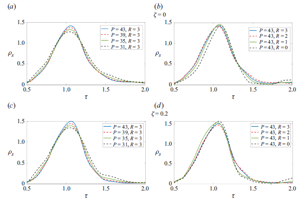
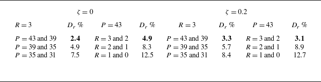
Galerkin expansion (4.12) up to mode numbers
 $P=43$
and
 $R=3$
is chosen. The above-mentioned simulation parameters ensured a convergence to less than 5 % variation in
 $\rho _{s}$
. A convergence study is given in Appendix B. Time domain simulations of (3.1)–(3.5) is performed using the Euler–Maruyama method with
 $\Delta \hat t=1\times 10^{-4}$
for
 $10^4$
non-dimensional time. The duration allows approximately
 $10^4$
vortex sheddings, leading to a converged statistics.
6. Results and discussion
The investigations on the vortex shedding dynamics are presented in two broad sections: (i) lock-in characteristics due to the variation of the five parameters (§ 7) and (ii) relevance of lock-in for combustion instability (§ 8). Our earlier paper (Mariappan Reference Mariappan2022) detailed the shedding dynamics for a range of harmonic excitation amplitudes
 $A$
and frequencies
 $f$
. Therefore, our discussion chiefly focuses on the effects of OU correlation time
 $\epsilon _n$
, amplitude
 $A_n$
and the multiplicative noise factor
 $\zeta$
.
7. Lock-in characteristics
The following subsections discuss the characteristic variation of the lock-in region for the parametric variations. First, we discuss the outcome of only the additive OU noise. The features of the shedding probability
 $\rho _s$
are discussed (§ 7.1). It is followed by the discussion on including multiplicative OU noise in § 7.2. Towards the end, the harmonic excitation is turned on and the occurrence of s-lock-in is discussed (§§ 7.3–7.4). An effort is made to link the s-lock-in region to only the OU noise excitation features.
7.1. Effects of additive OU noise
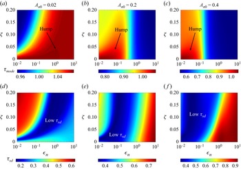
Figure 2 shows the p.d.f. (
 $\rho _s$
) of the shedding period
 $\tau$
for pure additive noise. Results for increasing noise amplitude
 $A_{n0}$
are depicted along the columns. We make three observations. The first one is broadening the
 $\rho _s$
p.d.f. with the increase in
 $A_{n0}$
for a given
 $\epsilon _n$
: an expected behaviour.
The second observation is the spreading of the p.d.f. (standard deviation) for increasing
 $\epsilon _n$
, for a given noise amplitude
 $A_{n0}$
(individual panels). It is nicely visible in the simulation for large noise amplitude (panel
 $c$
). The reason can be explained with the time domain simulation, shown in figure 3. Time evolution of the noise
 $\xi$
(panels a–c) and
 $\varGamma$
(panels d–f) for three different
 $\epsilon _n$
at
 $A_{n0}=0.1$
are plotted. The sudden drop in
 $\varGamma$
marks the shedding instances. At the lowest
 $\epsilon _n=0.01$
(panels a,d), there is almost no relaxation time for
 $\xi$
. Therefore,
 $\xi$
switches between positive and negative values quickly in comparison to the natural vortex shedding period. Therefore, the peak in
 $\rho _s$
is close to 1.0. At an intermediate
 $\epsilon _n=1.5$
(panels b,e), the larger relaxation time allows
 $\xi$
to stay on the positive or negative value side for longer. It allows quicker or slower, respectively, shedding sequences, leading to the spread in
 $\rho _s$
. The sequence appears to have intermittent fluctuations in the shedding frequency. It occurs when the natural shedding frequency is close to
 $\epsilon _n$
:
 $\epsilon _n\approx 1$
. The
 $\xi$
relaxes even slower for the largest
 $\epsilon _n=10$
(panels c,f), leading to a rise in the spread of
 $\rho _s$
(figure 3).
The third observation (related to the second one) is that the spread is skewed towards a lower shedding period for increasing
 $\epsilon _n$
and
 $A_{n0}$
. The skewed spread makes the p.d.f. non-Gaussian. Such p.d.f.s indicate the presence of intermittent fluctuations (Reuther & Kähler Reference Reuther and Kähler2020). The tail regions on either side of the p.d.f.
 $\rho _s$
captures the occasional events with either small or large vortex shedding period. Such intermittent fluctuations in the shedding period are observed in the time domain simulation of the circulation
 $\varGamma$
(figure 3
e). Therefore, the information regarding the transient dynamics (such as intermittent fluctuations) indeed appears in the p.d.f.
The mode (maximum probability of the shedding time period) of
 $\rho _s$
(white dashed curve in figure 2) indicates the gradual drop. It is observed even at
 $\zeta =0$
, indicating its cause is
 $\epsilon _n$
. An explanation in this regard is provided for the coloured OU noise. A formal solution in the absence of multiplicative noise (
 $\zeta =0$
) for (3.2) is as follows:
 \begin{equation} \xi (\tau )=\xi _0e^{-\tau /\epsilon _n}+\frac {A_{n0}}{\sqrt {2\epsilon _n}}e^{-\tau /\epsilon _n}\int _0^{\tau } e^{s/\epsilon _n}\eta _s\, {\textrm{d}}s, \end{equation}
where
 $\eta _s$
is the Gaussian white noise in the independent variable
 $s$
. Here,
 $\xi _0$
is the initial condition sampled from a Gaussian distribution of zero mean and
 $A_{n0}$
(noise amplitude of
 $\xi$
) standard deviation for each realisation. Inserting (7.1) in (3.1) and performing a formal integration leads to the time evolution of
 $\varGamma$
. The expression is valid between the shedding instances,
 \begin{align} \varGamma (\tau ) = &\int _0^\tau \frac {(1+u(\tau ^*))^2}{2}\,{\textrm{d}} \tau ^* +\xi _0 \epsilon _n\left (1-e^{-\tau /\epsilon _n}\right ) \nonumber\\&+\, \frac {A_{n0}}{\sqrt {\epsilon _n/2}}\int _0^\tau e^{-\tau ^*/\epsilon _n}\left (\int _0^{\tau ^*}e^{s/\epsilon _n}\eta _s \,{\textrm{d}}s \right )\,{\textrm{d}}\tau ^* .\end{align}
Using (7.2), an analytical expression for the ensemble average (angular brackets) of
 $\varGamma ^2$
can be written as
 \begin{equation} \big \langle \varGamma ^2(\tau )\big \rangle =\left [\int _0^\tau \frac {(1+u(\tau ^*))^2}{2}\,{\textrm{d}} \tau ^*\right ]^2+ 2A_{n0}^2\epsilon _n\left (\epsilon _n e^{-\tau /\epsilon _n}-\epsilon _n+\tau \right)\!,\quad \tau \gt 0. \end{equation}
The following inputs are used in the derivation of the above-mentioned expression:
 $\langle \xi _0\rangle =0,\,\langle \eta _s\eta _r\rangle =\delta (s-r)$
. Deterministic and stochastic (
 $S_c$
) contributions form the first and second terms in the
 $\langle \varGamma ^2\rangle$
expression. Additive noise appears as an additive correction
 $(S_c)$
to
 $\langle \varGamma ^2\rangle$
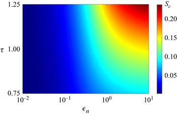
. A contour plot of
 $S_c$
with the shedding period
 $\tau$
for the range of
 $\epsilon _n$
is shown in figure 4 for a given noise amplitude
 $A_{n0}$
. Here,
 $S_c$
increases with
 $\epsilon _n$
. Therefore,
 $S_c$
quickens the circulation
 $\varGamma$
to reach the critical value
 $\varGamma _{\textit{sep}}$
. It results in a reduction in the maximum probability of the shedding time period (in an ensemble average sense). Therefore, the mode of
 $\rho _s$
shows a decreasing trend with
 $\epsilon _n$
. The trend becomes stronger, as
 $S_c \propto A_{n0}^2$
. The decrease in the mode of
 $\rho _s$
plays a crucial factor in the shape of the lock-in boundary, when excited with the harmonic signal (§ 7.3).
Contours of the stochastic term
 $S_c$
in the
 $\tau {-}\epsilon _n$
plane. The parameters are
 $A_{n0}=0.4,\,\zeta =0$
).

Variation of statistical measures of
 $\rho _s$
: mode (
 $\tau _{mode}$
) and standard deviation (
 $\tau _{\textit{sd}}$
) for various
 $\epsilon _n$
and
 $\zeta$
. Three noise amplitudes
 $A_{n0}=0.02,\,0.2$
and 0.4 are considered.

Note that the mode
 $\tau _{mode}$
in figures 2 and 5 is above 1 (natural shedding frequency) by
 ${\sim} 6\,\%$
for low
 $A_{n0}$
and
 $\epsilon _n$
. We expect it to be close to 1. We believe that the discrepancy is due to the 5 % variation cutoff in
 $\rho _s$
as the convergence criteria to decide the number of Galerkin modes
 $R,\,P$
(Appendix B).
7.2. Effects of multiplicative OU noise
The influence of the multiplicative noise in the shedding period statistics is presented in figure 5. Three representative noise amplitudes in the small (
 $A_{n0}$
= 0.02, panels a,d), medium (
 $A_{n0}$
= 0.2, panels b,e), and large (
 $A_{n0}$
= 0.4, panels c,f) values are chosen for illustration. Mode (
 $\tau _{mode}$
) and standard deviation of the probability density
 $\rho _s$
are plotted in panels (c) and (f), respectively. The varied parameters are the correlation time (
 $\epsilon _n$
) and the multiplicative noise factor (
 $\zeta$
).
Generally, the mode,
 $\tau _{mode}$
(panels
 $a{-}c$
) hovers around the natural vortex shedding frequency (1.0). A qualitative similarity in the features of
 $\tau _{mode}$
and
 $\tau _{\textit{sd}}$
distribution is observed for various
 $A_{n0}$
. For instance: (i) the presence of a hump in
 $\tau _{mode}$
(panels a–c) and (ii) the increase of low
 $\tau _{\textit{sd}}$
regions with
 $\epsilon _n$
and
 $\zeta$
. It indicates the underlying role of noise is the same for all
 $A_{n0}$
. Nevertheless, we notice quantitative differences. (i) In general, the mode
 $\tau _{mode}$
decreases with
 $A_{n0}$
, indicating the ensemble shedding period is quickened. A plausible reason is the factor
 $A_{n0}^2$
hastening
 $\langle \varGamma ^2\rangle$
(7.3) to reach the shedding circulation. (ii) Similarly, the standard deviation
 $\tau _{\textit{sd}}$
increases with higher noise levels (
 $A_{n0}$
values).
In the low-
 $\zeta$
case, the noise amplitude
 $A_n$
is almost constant (
 $\approx A_{n0}$
), leaving the effect of
 $\epsilon _n$
dominant. As briefed earlier, the monotonic decrease in the
 $\tau _{mode}$
results from the stochastic contribution
 $S_c$
. As one increases
 $\zeta$
, the noise intensity
 $A_n$
fluctuates according to the circulation
 $\varGamma$
. Since the dependence of
 $A_n^2$
with
 $\varGamma$
is quadratic (3.2), there is always an increase in the noise amplitude. As per the expression for
 $S_c$
, one expects a reduction in the shedding period with
 $\zeta$
for a given
 $\epsilon _n$
. Although we observe the above-mentioned trend for low noise level
 $A_{n0}=0.02$
(panel
 $a$
) at small
 $\epsilon _n$
, we observe a hump (non-monotonic behaviour, marked in panels a–c). We hypothesise that the hump is created due to the multiplicative nature of noise.
A rigorous mathematical explanation is not possible for the following reasons. (a) Since
 $A_n$
is a function of the circulation
 $\varGamma$
, (3.1)–(3.2) become coupled. Therefore, a formal solution for the noise
 $\xi$
similar to (7.2) for pure additive noise is not possible. (b) Equation (3.2) becomes nonlinear in
 $\varGamma$
through the term
 $A_n$
. The above-mentioned reasons prevent us from obtaining an equation similar to (7.3), where the effect of noise on the mode of
 $\rho _s$
is discernible through
 $S_c$
. For multiplicative noise, a plausible heuristic argument is as follows. As mentioned in reason (a), both
 $\xi$
and
 $\varGamma$
evolve simultaneously, leading to a feedback loop (similar to heat release rate and acoustics in thermoacoustic interaction). The loop either accelerates or decelerates the vortex-shedding process, depending on
 $\epsilon _n$
. The noise correlation time
 $\epsilon _n$
(can be compared with the time delay in thermoacoustics) acts as a memory effect of the past noise value
 $\xi$
. Similar to thermoacoustic interaction, the acceleration (low-
 $\tau _{mode}$
regions) or deceleration (high-
 $\tau _{mode}$
regions) depends on
 $\epsilon _n$
non-monotonically, leading to the observed hump in
 $\tau _{mode}$
. The location of the hump occurs around a particular
 $\epsilon _n$
and it strongly depends on
 $A_{n0}$
. High noise levels dominate the effect of
 $\epsilon _n$
. Therefore, the region (figure 5
a−c) of accelerated vortex shedding (low
 $\tau _{mode}$
) expands, pushing the hump towards the low
 $\epsilon _n$
values.
Panels (d–f) show the standard deviation (
 $\tau _{\textit{sd}}$
) of
 $\rho _s$
. As in the previous paragraph, one expects a monotonic rise in
 $\tau _{\textit{sd}}$
with
 $\zeta$
due to the quadratic nature of the multiplicative noise amplitude. However, the multiplicative noise affects the vortex dynamics non-trivially, leading to non-monotonic variation of
 $\tau _{\textit{sd}}$
too. In particular, we observe regions of low
 $\tau _{\textit{sd}}$
(blue region). The combination of the low
 $\tau _{\textit{sd}}$
region, along with the region of
 $\tau _{mode}$
(figure 2) close to the harmonic excitation time period, aids in determining the stochastic-lock-in region, described in the following subsection.
7.3. Effects of simultaneous OU noise and harmonic excitation
A deterministic version of the vortex-shedding model (
 $A_{n0}=0$
) represents a self-sustained oscillator with frequency 1, also termed a period-1 solution in the parlance of a dynamical system. When excited with a harmonic external forcing, the shedding frequency and its dynamical pattern change (from the period-1 solution). At appropriate excitation amplitudes and frequencies, the period-1 solution reappears (dynamic bifurcation occurs). This time, the shedding frequency is the exciting frequency. The phase difference between the shedding and the excitation signals is also maintained. The phenomenon is termed a 1 : 1 phase lock-in. In general, the shedding and excitation frequency ratio can be rational
 $q/p$
(
 $p,q$
are integers). It is defined as
 $p:q$
lock-in. Detailed theoretical investigation in relation to thermoacoustics is given by Britto & Mariappan (Reference Britto and Mariappan2019, Reference Britto and Mariappan2021).
In the stochastic counterpart, lock-in is identified by the phase of the eigenvalues of the transition probability matrix
 $\boldsymbol{T}$
. The eigenvalues are ordered in descending order of their absolute values. The largest (first) eigenvalue of
 $\boldsymbol{T}$
always equals 1, leading to a stationary probability distribution
 $\rho _s$
of the vortex-shedding time period. The 1 : 1 stochastic lock-in occurs when the phase of the second eigenvalue becomes zero. The phase of the higher eigenvalues determines higher-order s-lock-in. Our earlier result (Mariappan Reference Mariappan2022) shows that 1 : 1 s-lock-in provides the most favourable condition for combustion instability in the presence of Gaussian white noise. It is also found to be true when re-interpreted with our previous experiments (Britto & Mariappan Reference Britto and Mariappan2023). Furthermore, since the present paper is focused on studying the effects of colour and multiplicative noise, we restrict our attention to 1 : 1 s-lock-in, for limiting the range of harmonic excitation parameters,
 $f,\,A$
. We discuss the shape of the s-lock-in boundary in the harmonic excitation parameters plane,
 $A{-}f$
, followed by the noise parameters space,
 $A_{n0},\,\epsilon _n,\,\zeta$
.
7.3.1. Lock-in boundary in the harmonic excitation parameters
$(A,\,f)$
plane

Figure 6 shows the contours of the second eigenvalue phase
 $(\theta _2)$
in the harmonic excitation parameter space for three different noise amplitudes
 $A_{n0}$
(rows) and correlation times
 $\epsilon _n$
(columns). Additive noise is considered,
 $\zeta =0$
. The white curve indicates the s-lock-in boundary, inside which
 $\theta _2=0$
. At the noise amplitude
 $A_{n0}=0.02$
, the lock-in boundary remains almost the same for all the correlation times
 $\epsilon _n$
. The feature is due to the low noise level.
Contour plots detailing the variation of the phase
 $\theta _2$
of the second eigenvalue of the transition probability matrix
 $\boldsymbol{T}$
for various
 $A,\,f$
parameter combinations at
 $\zeta =0$
. Continuous white and dashed green curves represent the 1 : 1 s-lock-in boundary for
 $\zeta =0$
and 0.2, respectively.

At the intermediate
 $A_{n0}=0.2$
(panels b,e,h) and high
 $A_{n0}=0.4$
(panels c,f,i) noise levels, the boundary shape strongly depends on
 $\epsilon _n$
. Notably, the boundary is shifted to the higher excitation frequency (mostly
 $f\gt 1$
) for
 $A_{n0}=0.2$
. A reasonable connection between the lock-in boundary shape and the harmonically unexcited
 $\tau _{mode},\,\tau _{\textit{sd}}$
(figure 5) contours can be made as follows. The maximum probability of the shedding time period,
 $\tau _{mode}$
(frequency) decreases (increases) for higher values of
 $\epsilon _n$
. In this region, the excitation frequency
 $f$
coincides more often with
 $1/\tau _{mode}$
. Furthermore, the
 $\tau _{\textit{sd}}$
has lower values in the higher
 $\epsilon _n$
region (refer to
 $\zeta =0$
in figure 5). A combination of the above-mentioned two factors leads to a shift and change in the lock-in boundary shape for intermediate noise amplitudes,
 $A_{n0}=0.2$
.
The lock-in region almost ceases to exist (
 $\epsilon _n=0.77$
, panel
 $h$
in figure 6) and reappears (
 $\epsilon _n=10$
, panel
 $i$
) for the highest noise amplitude
 $A_{n0}=0.4$
. The cessation at
 $\epsilon _n=0.77$
can be attributed to the non-proximity between the values of
 $1/\tau _{mode}$
(figure 5
b) and
 $f$
. It is further fuelled by high values of
 $\tau _{\textit{sd}}$
at the regions where the above-mentioned proximity occurs. The reappearance of the lock-in region at
 $\epsilon _n=10$
(figure 6
i) is due to the low
 $\tau _{\textit{sd}}$
and proximity between
 $1/\tau _{mode}$
and
 $f$
.
Green dashed curves in figure 6 represent the lock-in boundary in the presence of multiplicative noise
 $\zeta =0.2$
. Since
 $\zeta$
has a substantial impact on
 $\tau _{mode}$
and
 $\tau _{\textit{sd}}$
(figure 5), we expect a significant difference in the lock-in boundary due to the multiplicative noise. Since the difference in
 $\tau _{mode}$
and
 $\tau _{\textit{sd}}$
between
 $\zeta =0$
and
 $0.2$
is significant for the lowest
 $\epsilon _n=0.01$
(figure 5), we observe a noteworthy difference in the lock-in boundaries in figure 6 (panels a,d,g). Furthermore, the same difference decreases with an increase in
 $\epsilon _n$
(figure 5), the lock-in boundary with multiplicative noise appears closer to the pure additive noise case for intermediate and high
 $\epsilon _n$
(last two columns of figure 6).
A practical observation from the above-mentioned exercise is that the s-lock-in location in the parameter space during harmonic excitation can be approximately identified from the (i) closeness of the mode of the shedding period to the harmonic excitation period and (ii) standard deviation of the shedding period, in the presence of only background turbulent fluctuations. The above-mentioned outcome is found to be common to both additive and multiplicative noise. Similar outcomes were used to detect an impending combustion instability (for example, Nair & Sujith Reference Nair and Sujith2014) and system identification (for example, Lee et al. Reference Lee, Kim, Gupta and Li2021) from the response of the system to turbulent fluctuations.
7.3.2. Lock-in boundary in the OU noise parameters
$(A_{n0},\,\epsilon _n)$
plane

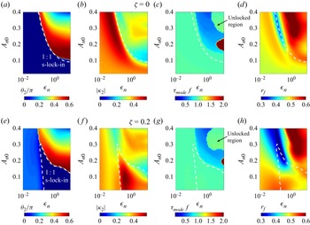
Figure 7 shows the occurrence of s-lock-in for various
 $\epsilon _n$
and
 $A_{n0}$
considering an additive noise
 $(\zeta =0)$
(panels a–d) and including a multiplicative noise (panels e–h). The exciting amplitude and frequency are the same:
 $A=0.25$
and
 $f=0.9$
. Lock-in is observed in the corresponding deterministic (
 $A_{n0}=0$
) case (refer to figure 6b of Britto & Mariappan Reference Britto and Mariappan2019).
Contour plots detailing the variation of the phase
 $\theta _2$
(panels a,e) and the absolute value
 $|\kappa _2|$
(panels b, f) of the second eigenvalue of the transition probability matrix
 $\boldsymbol{T}$
. The next two columns represent the scaled mode
 $\tau _{mode} f$
of the p.d.f.s
 $\rho _s$
and the relative fluctuations
 $r_f$
. The harmonic excitation frequency and amplitude are
 $f=0.9$
and
 $A=0.25$
, respectively. The white dashed curve in all the panels represents the 1 : 1 s-lock-in boundary. The top and bottom row panels represent additive
 $\zeta =0$
and multiplicative noise
 $\zeta =0.2$
, respectively.

Considering the case of additive noise first (panels a–d), contours of
 $\theta _2$
are plotted. The dashed white curve indicates the s-lock-in boundary. At low noise amplitudes
 $A_{n0}\lt 0.09$
, s-lock-in continues to exist for all
 $\epsilon _n$
. It ceases to occur for large
 $\epsilon _n$
at higher noise amplitudes, due to the spread in the unforced shedding period distribution (figure 5). The cessation region widens with the rise in
 $A_{n0}$
. The white dashed curve (s-lock-in boundary) represents a stochastic bifurcation. It is defined as a transition point where the phase
 $\theta _2$
of the second eigenvalue of the transition probability matrix
 $\boldsymbol{T}$
becomes zero, as a parameter is varied. The transition of
 $\theta _2$
equalling zero is to identify 1 : 1 s-lock-in only, which is studied exclusively in this paper. Other orders of s-lock-in are identified when
 $\theta _2$
takes specific rational multiples of
 $\pi$
(Plesser & Tanaka Reference Plesser and Tanaka1997). Across a stochastic bifurcation, there is a qualitative change in the shedding period distribution
 $\rho _s$
(discussed in § 7.3.2 and shown in figure 8).
P.d.f. of the shedding time period
 $\rho _s$
at a
 $\epsilon _n$
and
 $A_{n0}$
are shown in the first two columns:
 $\epsilon _n=0.77$
and
 $A_{n0}=0.15$
respectively. Vertical dashed lines locate the boundary of 1 : 1 s-lock-in. External excitation amplitude and frequency are the same as in figure 7.

Figure 7
 $(b)$
shows the absolute value
 $(|\kappa _2|)$
contours of the second eigenvalue. Its value indicates the strength of the s-lock-in. Near the boundary (white dashed curve),
 $|\kappa _2|$
smoothly reduces between the s-lock-in and unlocked region. Panel (
 $c$
) provides a similar insight regarding the shedding period. The contour of the product of mode
 $(\tau _{mode})$
of
 $\rho _s$
and the excitation frequency
 $f$
equals 1 (green shade) in the s-lock-in region. Furthermore, the relative fluctuation
 $r_f$
(ratio of standard deviation
 $\tau _{\textit{sd}}$
and mean of
 $\rho _s$
) is lower in the s-lock-in region and rises across the lock-in boundary. Large
 $r_f$
(panel d) leads to the unlocked state, although
 $\tau _{mode}f$
equals to 1 in a patch (marked in panel
 $c$
) at high values of
 $A_{n0},\,\epsilon _n$
.
The presence of multiplicative noise (panels e–h) shrinks the s-lock-in region further (panel
 $a$
). The phase
 $\theta _2$
takes values close to 0 (but not 0) at low
 $\epsilon _n$
. Hence, the system is close to s-lock-in:
 $\tau _{mode}f=1$
(panel g). Other than the above-mentioned differences, the qualitative features of
 $|\kappa _2|,\,\tau _{mode}f,\,r_f$
remain the same as those of the additive noise case.
The shrink in the s-lock-in region (at high
 $A_{n0}$
) is observed at the location of a combination of low
 $\tau _{mode}$
with respect to the harmonic excitation time period
 $1/f=1.1$
and high standard deviation
 $\tau _{\textit{sd}}$
observed at
 $\zeta =0.2$
for zero harmonic excitation (figure 5). Therefore, we expect that multiplicative noise does not bring a new mechanism (dynamics), at least for s-lock-in. Intermittency or skewed
 $\rho _s$
distribution is observed for pure additive noise too, § 7.1.
Figure 8 shows the path the system takes as it crosses the s-lock-in boundary. It is illustrated through the contours of the p.d.f.
 $\rho _s$
for a given
 $\epsilon _n=0.77$
(panel a) and
 $A_{n0}=0.15$
(panel b). The other variables
 $A_{n0}$
and
 $\epsilon _n$
are varied respectively in the two panels. The product
 $\tau f$
is plotted for the p.d.f. random variable. For low noise amplitudes (panel a), where s-lock-in occurs, the
 $\rho _s$
distribution is narrow, peaking close to
 $\tau f=1$
(white horizontal line). The spread in
 $\rho _s$
increases as one approaches the s-lock-in boundary (vertical dashed line). Crossing the boundary leads to the peak shifting away from the excitation frequency. A similar situation occurs when
 $\epsilon _n$
(panel b) increases and for the case of multiplicative noise (not shown for brevity).
7.4. Effects of harmonic excitation frequency
The previous subsection dealt with considering a particular harmonic excitation frequency
 $f=0.9$
. The vortex shedding or acoustic frequency (essentially
 $f$
) is often altered to keep the combustor in the unlocked state (Lieuwen Reference Lieuwen2012), thereby avoiding combustion instability. Therefore, we study the effects of noise parameters at various harmonic excitation frequencies
 $f$
.
Figure 9 shows the extent and strength of 1 : 1 s-lock-in in the
 $\zeta {-}\epsilon _n$
plane. Harmonic excitation frequency,
 $f$
, increases from the left to right panels. Panels (a)–(d) show the phase
 $\theta _2$
contours. The white curve in each panel indicates the boundary inside which
 $\theta _2=0$
and 1 : 1 s-lock-in occurs. In panels (a) and (b), where
 $f\lt 1$
, the size of the s-lock-in region increases as
 $f$
approaches 1. The genesis of the s-lock-in region occurs, where
 $\epsilon _n \sim 0.1$
(panel
 $a$
). However, for
 $f\gt 1$
(panels
 $c,\,d$
), it is pushed towards higher values of
 $\epsilon _n$
. The lock-in region also decreases as
 $f$
moves away from 1.
Top and bottom row panels show the variation of the phase
 $\theta _2$
(normalised with
 $\pi$
) and absolute
 $|\kappa _2|$
of the second eigenvalue of
 $\boldsymbol{T}$
in the
 $\zeta {-}\epsilon _n$
plane. The continuous white curve in each panel marks the boundary of the 1 : 1 s-lock-in region. Each panel represents the harmonic external excitation frequencies on either side of the natural vortex shedding frequency. Harmonic excitation and noise amplitudes are kept constant at
 $A=0.25$
and
 $A_{n0}=0.15$
, respectively. Four different harmonic excitation frequencies
 $f=0.8,\,0.9,\,1.1$
and 1.2 are considered.

The above-mentioned observation can be connected with the mode
 $(\tau _{mode})$
contours of the shedding frequency without harmonic forcing (figure 5
a), discussed previously in § 7.1. For
 $f\lt 1$
in figure 9(a, b), lock-in is observed in the region where
 $\tau _{mode}\gt 1$
in figure 5(a) (at
 $\epsilon _n \sim 0.1$
). It indicates that lock-in occurs in the region where the maximum probability of the shedding period is close to the external harmonic excitation period. Using the same reasoning, one anticipates lock-in for
 $f\gt 1$
(figure 9
c, d) would occur for large and small (at least for
 $\zeta \gt 0.05$
) values of
 $\epsilon _n$
. However, we observe lock-in only at large
 $\epsilon _n$
in figure 9(c, d). At small
 $\epsilon _n$
, the standard deviation
 $\tau _{\textit{sd}}$
(figure 5
b) is large leading to the disappearance of lock-in.
Figure 9(e–h) displays the
 $|\kappa _2|$
contours. The value of
 $|\kappa _2|$
denotes the strength of the s-lock-in. At
 $f=0.8$
(panel e),
 $|\kappa _2|$
takes relatively high values in the s-lock-in region. Its value further increases for
 $f=0.9$
and strengthens the s-lock-in region. However, in the
 $f\gt 1$
region, low values of
 $|\kappa _2|$
represent a weak s-lock-in. The analysis in the section concludes that the s-lock-in region is intense for
 $f\lt 1$
(excitation frequency is lower than the natural vortex shedding frequency) and it appears near
 $\epsilon _n \sim 0.1$
.
Figures 6–9 represent the s-lock-in region in various parameter space:
 $A,\,f,\,A_{n0},\,\epsilon _n$
and
 $\zeta$
. Lock-in is accompanied by combustion instability in many combustors (for example, Poinsot et al. Reference Poinsot, Trouve, Veynante, Candel and Esposito1987, Lieuwen Reference Lieuwen2012, Singh & Mariappan Reference Singh and Mariappan2021). Therefore, excluding the lock-in region from the above-mentioned figures serves as a safe operating map in the parameter space. Subsequently, it can also aid as a design guideline in the parameter selection of new combustors.
8. Relevance to combustion instability
Section 7 described the s-lock-in characteristics and the reasoning for the same. The present section discusses its implications on combustion instability.
The unsteady heat release rate feedback during combustion caused by vortex shedding depends on two factors: (i) shedding period
 $\tau$
and (ii) strength of the vortex
 $\varGamma _{\textit{sep}}$
. Considering the first factor, parameter regions of 1 : 1 s-lock-in are favourable for combustion instability (Britto & Mariappan Reference Britto and Mariappan2023). Moving on to the second factor,
 $\varGamma _{\textit{sep}}$
is a random variable taking values between
 $(1\pm A)/2$
(since
 $|u|=A$
). Here,
 $\varGamma _{\textit{sep}}=0.5$
without external harmonic forcing. Inclusion of the forcing changes
 $\varGamma _{\textit{sep}}$
according to the shedding phase instance of
 $u$
. Here,
 $\varGamma _{\textit{sep}}\gt 0.5$
is favourable for combustion instability, as its value is more than the unforced state.
The two above-mentioned combinations for favouring combustion instability are explored in the light of s-lock-in (combined role of harmonic excitation and OU noise) and stochastic resonance. As stated towards the end of the previous section, the s-lock-in region should be avoided to prevent combustion instability. Since detailed s-lock-in maps have already been discussed, we focus our attention on stochastic resonance. However, the s-lock-in boundary is used to understand the combined effects of the two phenomena.
Stochastic resonance is also a noise-induced phenomenon, where noise amplifies the output response to the input harmonic excitation
 $u(t)$
. It is quantified by signal-to-noise ratio (SNR), defined as the ratio of spectral powers in the system response to the noise at the input frequency
 $f$
. The system response is chosen as the vortex circulation (
 $\varGamma _v$
) shed at time
 $t_m$
,
 $\varGamma _v=\sum _{m=0}^{\infty }\delta (t-t_m)\varGamma _{\textit{sep}}$
. The SNR is evaluated from the spectral powers in the response
 $\varGamma _v$
during the presence
 $(S_{\varGamma })$
and absence
 $(S_{\varGamma ,N})$
of the harmonic excitation at the excitation circular frequency
 $\omega =2\pi f$
. The SNR expression is
 $\textrm{SNR}=S_{\varGamma }/S_{\varGamma ,N}-1$
. Subtraction by 1 removes the noise component in the spectral power
 $S_{\varGamma }$
. The spectral power
 $S_{\varGamma }$
is defined in the standard form (Priestley Reference Priestley1981):
 $S_{\varGamma }(\omega ) = ({1}/{\pi T_0})\langle |\int _0^{T_0}\varGamma _ve^{i\omega t}\,{\textrm{d}}t|^2\rangle$
with
 $i=\sqrt {-1}$
, where angular
 $\langle \,\rangle$
and vertical
 $|\,|$
brackets indicate ensemble average and absolute value, respectively. Here,
 $T_0$
is the observation time. It is necessary to set it longer than the natural shedding or excitation periods. We use a value
 $T_0=200$
. An analytical solution is possible to obtain
 $S_{\varGamma }$
at the excitation circular frequency
 $\omega$
. The expression for
 $S_{\varGamma }$
is in Appendix A of Mariappan (Reference Mariappan2022). Matrix multiplication is involved in the expression and, therefore, no numerical methods are required.
The same paper (Mariappan Reference Mariappan2022) also found that the maximum SNR is approximately 1.5 in the presence of additive Gaussian white noise and therefore concluded that stochastic resonance may not be a threat to the occurrence of combustion instability. A re-examination of the above-mentioned conclusion is made for multiplicative colour noise. The current work involves three noise parameters
 $A_{n0},\,\epsilon _n$
and
 $\zeta$
. The SNR is normalised with a factor
 ${\textrm{SNR}}_{G}$
. Here,
 ${\textrm{SNR}}_{G}$
is the SNR at the lowest values of
 $\epsilon _n=0.01$
and
 $\zeta =0$
, which imitates Gaussian white noise. It allows a comparison of stochastic resonance with the previously examined additive Gaussian white noise case. The lowest noise amplitude
 $A_{n0}=0.02$
is chosen.
Variation of the normalised signal-to-noise ratio
 $(\textrm{SNR}/\textrm{SNR}_G)$
with noise amplitude
 $A_{n0}$
and correlation time
 $\epsilon _n$
for additive (panel a) and multiplicative noise (panel e). The white curve represents the s-lock-in boundary. Dashed horizontal lines in panel (a) represent the three amplitudes, described in the subsequent panels. Contours of
 $\varGamma _{\textit{sep}}$
probability (
 $\rho _{\varGamma _{\textit{sep}}}$
) with
 $\epsilon _n$
at three noise amplitudes (increasing in their values) are shown in panels (b−d). The parameters correspond to figure 7(b, f).

8.1. Contribution of stochastic resonance and s-lock-in
The results of stochastic resonance and distribution of
 $\varGamma _{\textit{sep}}$
in relation to combustion instability are shown in figure 10. Additive noise is considered in the first four panels. Panel (a) shows a patch of high normalised SNR in the
 $A_{n0}{-}\epsilon _n$
plane, indicating a strong stochastic resonance. Coloured noise promotes stochastic resonance, as reported by Nozaki, Collins & Yamamoto (Reference Nozaki, Collins and Yamamoto1999) for biological neurons. In the plot, stochastic resonance occurs at
 $A_{n0}=0.25,\,\epsilon _n=0.34$
. Many industrial gas turbine combustors operate in the above-mentioned turbulent noise parameter range (Hosseinalipour et al. Reference Hosseinalipour, Fattahi, Khalili, Tootoonchian and Karimi2020). Therefore, at first sight, stochastic resonance appears favourable for the occurrence of combustion instability in the practical combustors.
However, the 1 : 1 s-lock-in region (boundary shown by the continuous white curve) does not engulf the high stochastic resonance patch. A 1 : 1 s-lock-in is a period-1 dynamical solution for the shedding period
 $\tau$
, superimposed by stochastic fluctuations. The period-1 solution is centred around the excitation frequency (figure 7
c). An essential ingredient of a higher periodic solution begins to appear at the lock-in boundary (Balanov et al. Reference Balanov, Janson, Postnov and Sosnovtseva2008). Stochastic resonance does peak near the lock-in boundary.
8.2. Contribution of shedding circulation
$\varGamma _{\textit{sep}}$

The probability
 $(\rho _{\varGamma _{\textit{sep}}})$
distribution of
 $\varGamma _{\textit{sep}}$
at three locations, low
 $A_{n0}=0.07$
, where s-lock-in occurs for all
 $\epsilon _n$
(panel b), medium
 $A_{n0}=0.25$
passing through the location of maximum stochastic resonance (panel c) and high
 $A_{n0}=0.38$
(panel d), where s-lock-occurs partly are plotted.
At low
 $A_{n0}$
,
 $\varGamma _{\textit{sep}}$
takes high probability (white regions) near
 $(1+A)/2$
for small
 $\epsilon _n\lessapprox 1$
, indicating a favourable condition for combustion instability. However,
 $\varGamma _{\textit{sep}}$
high probability switches to the lower side (near
 $(1-A)/2$
) for
 $\epsilon _n\gtrapprox 1$
. Therefore,
 $\epsilon _n$
strongly influences the occurrence of combustion instability in the lock-in region.
In the medium
 $A_{n0}$
(panel c) case, a similar switch in
 $\varGamma _{\textit{sep}}$
probability occurs. The switch is closer to the location of maximum stochastic resonance. Therefore, stochastic resonance appears to play a favourable role for combustion instability. At the high
 $A_{n0}$
(panel d), high probability regions are both near
 $\varGamma _{\textit{sep}}=(1+A)/2$
and
 $(1-A)/2$
for
 $\epsilon \ll 1$
. Large
 $\epsilon _n$
values lead to high probability close to 0.5: the unperturbed shedding circulation.
Combining the above-mentioned observations on lock-in boundary and vortex circulation probability, we conclude that coloured noise promotes stochastic resonance significantly (approximately 10 times) compared with Gaussian white noise. The circulation (
 $\varGamma _{v}$
) at the time of vortex shedding is proportional to the unsteady heat release produced by the vortex (Matveev & Culick Reference Matveev and Culick2003). Since SNR is calculated based on
 $\varGamma _{v}$
, an approximate tenfold (figure 10
a) increase in the unsteady heat release is observed: a physical observable. Since the rise is significant compared with the Gaussian white noise (Mariappan Reference Mariappan2022), we expect coloured noise may play a crucial role in the occurrence of combustion instability through stochastic resonance. However, the above-mentioned argument is incomplete, as the occurrence of combustion instability also depends on the phase difference between the pressure and heat release rate oscillations (Rayleigh Reference Rayleigh1878). It requires two-way thermoacoustically coupled analysis (beyond the scope of the present paper). In any case, the tenfold rise in the unsteady heat release may still pose a threat to instability in practical combustors (Lieuwen & Yang Reference Lieuwen and Yang2005).
Adding the multiplicative noise (of highest
 $\zeta =0.2$
), the normalised SNR dropped to
 ${\sim}1.5$
(panel
 $e$
). Therefore, multiplicative noise does not promote stochastic resonance and, in turn, combustion instability. Other plots related to
 $\varGamma _{\textit{sep}}$
probability remain qualitatively similar to the additive noise case and therefore are omitted for brevity.
The highest multiplication factor
 $\zeta =0.2$
is chosen based on the simulations of Wilczek & Friedrich (Reference Wilczek and Friedrich2009) (refer to discussion in § 5). From figure 10, it is unclear whether the trend of normalised SNR monotonically decreases with
 $\zeta$
for intermediate values
 $(0\lt \zeta \lt 0.2)$
or completely suppresses the stochastic resonance at values
 $\zeta \gt 0.2$
. Performing simulations in the three-parameter space,
 $A_{n0},\,\epsilon _n$
and
 $\zeta$
, is computationally expensive. However, given the monotonic effects of
 $\zeta$
in the previous figures 5 and 9, we expect the same to hold true in stochastic resonance.
8.3. Possible passive control strategy
Based on the discussions made in §§ 7.3.1–8, it is possible to avoid s-lock-in by passively controlling the parameters
 $f,\,\epsilon _n$
and
 $\zeta$
. Other parameters are as follows. (i) Noise amplitude
 $A_{n0}$
and the correlation time
 $\epsilon _n$
are mostly determined by the incoming flow. They are known parameters. (ii) Acoustic oscillation amplitude
 $A$
is a result of thermoacoustic interaction. Therefore, the three parameters cannot be tuned for a passive control strategy. The author believes that there are two options available for passive control. (a) The easiest choice is to alter the frequency ratio
 $f$
, according to the s-lock-in maps shown in figures 6 and 9. It is achieved, either by tweaking the combustor (natural acoustic frequency, for example, Han et al. Reference Han, Han, Wang and Li2022) or burner (vortex shedding frequency, for example, Griffin Reference Griffin1985) geometries. (b) A second option is to alter the multiplicative noise factor
 $\zeta$
. Combustor liners can be built using acoustic metamaterials. They are inherently nonlinear in sound absorption (Gao et al. Reference Gao, Zhang, Deng, Guo, Cheng and Hou2022). Such nonlinear materials can be engineered to manipulate
 $\zeta$
. Although such materials are yet to be tested in the harsh environment of a combustor, future possibilities do exist.
9. Parallels from the past investigations
The present paper indirectly relates the occurrence of 1 : 1 s-lock-in to thermoacoustic instability in noisy combustors in evolving vortex shedding. Although experimental evidence for the validity of the results is unavailable to the best of the author’s knowledge, it is possible to draw parallels with previous simulations and experimental observations. (i) The earliest work by Waugh & Juniper (Reference Waugh and Juniper2011a
) indicates that additive and multiplicative noise result in qualitatively similar behaviour in thermoacoustic systems. We do observe with increase in
 $\zeta$
, the qualitative behaviour of the plots (figures 5–7, 9, 10) does not change. (ii) Multiplicative noise reduces the extent of the s-lock-in region (figure 7) and, therefore, thermoacoustic instability, corroborating with Li et al. (Reference Li, Xu, Li, Pang, Li and Zhang2023). (iii) S-lock-in features at large noise correlation time
 $\epsilon _n$
(figures 5, last column panels of figures 6, 7, 9) largely remain the same quantitatively, irrespective of the multiplicative noise factor
 $\zeta$
. It indicates lesser effects of the multiplicative nature of noise on the statistical features of thermoacoustic instability at large
 $\epsilon _n$
. In parallel, early warning indicators of thermoacoustic instability, such as the Hurst exponent, coherence factor and variance, do perform almost equally well at large
 $\epsilon _n$
(Vishnoi & Kabiraj Reference Vishnoi and Kabiraj2024). These indicators also depend on the statistical features of the acquired pressure/heat release time series.
10. Limitation of present study and future directions
The above-described results provide vital conclusions regarding vortex–acoustic lock-in and stochastic resonance in a noisy combustor in relation to combustion instability. Nevertheless, the paper has the following limitations. The paper used the low-order model (deterministic part) of Matveev & Culick (Reference Matveev and Culick2003) for vortex shedding behind bluff bodies. Although Fage & Johansen (Reference Fage and Johansen1927) experimentally confirmed the reasonability of the model, it is unclear about its performance for complex geometries as encountered in practical systems (Lieuwen & Yang Reference Lieuwen and Yang2005). Furthermore, the noise follows the OU process with a multiplicative component, having a factor
 $\zeta$
. Apart from clarity in the range of other noise parameters (§ 5), the chosen range for
 $\zeta$
is from the simulation of a canonical configuration (Wilczek & Friedrich Reference Wilczek and Friedrich2009). Again, it may not represent the conditions of practical combustors. Given the above-mentioned limitations, the presented conclusions can be considered as a first design guideline for building stable operating combustors. A future outlook will be to perform high-fidelity simulations or detailed experimental diagnostics to accurately quantify the unknown noise parameters, thereby obtaining a better grip on s-lock-in and stochastic resonance phenomena.
11. Conclusion
The paper investigates the stochastic dynamics of the vortex shedding phenomenon in the presence of external harmonic and multiplicative, coloured noise excitation. The study pertains to understanding combustion instability due to vortex shedding in turbulent practical combustors. External harmonic excitation represents the combustor acoustic field, while the multiplicative coloured noise is a surrogate for the turbulent flow fluctuations. The Ornstein–Uhlenbeck process is used to describe coloured noise. The probability density function of the vortex shedding time period (
 $\rho _s$
) is obtained by numerically simulating a low-order model in the Fokker–Planck framework. Stochastic lock-in is studied extensively for various harmonic and noise excitation parameters.
The following are the salient conclusions. (i) The noise correlation time significantly affects
 $\rho _s$
. The most probable vortex shedding time period (mode of
 $\rho _s, \tau _{mode}$
) and the standard deviation (
 $\tau _{\textit{sd}}$
) of
 $\rho _s$
decrease and increase, respectively, with the correlation time. (ii) Multiplicative noise makes the above-mentioned trend non-trivial. (iii) The proximity of
 $\tau _{mode}$
to the excitation time period, along with low
 $\tau _{\textit{sd}}$
, forms sites of stochastic lock-in (s-lock-in) in the parameter space. The shape and size of the s-lock-in boundary change in a non-trivial manner with noise correlation time and amplitude. (iv) A tenfold rise in the stochastic resonance is observed compared with the Gaussian white noise. Therefore, it may play a crucial role in the occurrence of combustion instability. Multiplicative noise lowers the amount of stochastic resonance. The above-mentioned conclusions can serve as a design guideline to prevent combustion instability through lock-in in practical combustors.
Declaration of interests
The authors report no conflict of interest.
Acknowledgement
The author is grateful to the high-performance computing facility at the Indian Institute of Technology Kanpur for some of the presented simulations.
Funding
The author thanks the partial financial support from the Science & Engineering Research Board (Grant Number CRG/2019/000500) and Aeronautics Research & Development Board (Grant Number ARDB/AE/2021497).
Appendix A. Functional forms of Galerkin integrals
 \begin{align} I^{\alpha }_{pqrs}&=\delta ^k_{rs}\left (\int _{\hat \varGamma =0}^{\infty }\frac {{\textrm{d}}\psi _p}{{\textrm{d}} \hat \varGamma }\psi _q \,{\textrm{d}}\hat \varGamma \right)\!, \end{align}
 \begin{align} I^{\beta }_{pqrs}&=\delta ^k_{rs}\left (\int _{\hat \varGamma =0}^{\infty }\hat \varGamma \frac {{\textrm{d}}\psi _p}{{\textrm{d}} \hat \varGamma }\psi _q {\textrm{d}}\hat \varGamma \right ) \end{align}
 \begin{align} I^{\gamma }_{pqrs}&=\left (\int _{\hat \xi =-\infty }^{\infty }\hat \xi \varphi _r \varphi _s {\textrm{d}}\hat \xi \right )\left (\int _{\hat \varGamma =0}^{\infty }\frac {{\textrm{d}}\psi _p}{{\textrm{d}} \hat \varGamma }\psi _q {\textrm{d}}\hat \varGamma \right ) \end{align}
 \begin{align} I^{\delta }_{pqrs}&=\left (\int _{\hat \xi =-\infty }^{\infty }\frac {d}{{\textrm{d}} \hat \xi }\big (\hat \xi \varphi _r\big )\varphi _s{\textrm{d}}\hat \xi \right )\delta ^k_{pq} \end{align}
 \begin{align} I^{\varUpsilon }_{pqrs}&=\left (\int _{\hat \xi =-\infty }^{\infty }\frac {d^2\varphi _r}{{\textrm{d}} \hat \xi ^2}\varphi _s{\textrm{d}}\hat \xi \right )\left (\int _{\hat \varGamma =0}^{\infty }\big (1-\hat \varGamma \big )^2\psi _p\psi _q{\textrm{d}}\hat \varGamma \right ) \end{align}
 \begin{align} I^{\nu }_r&=\int _{\hat \xi =-\infty }^{\infty }\varphi\, {\textrm{d}}\hat \xi, \end{align}
 \begin{align} I^{\varsigma }_p&=\int _{\hat \varGamma =0}^{\infty }\psi \,{\textrm{d}}\hat \varGamma, \end{align}
where
 $p,q=1,3,5,\ldots$
and
 $r,s=0,1,2,\ldots$
. The subscripts
 $p{-}s$
in
 $I$
are suppressed in (4.13) and (4.15) of the main text for brevity.
P.d.f.
 $\rho _s$
of the shedding time period
 $\tau$
for various combinations of
 $P$
(panels a,c) and
 $R$
(panels b,d). The exercise is performed to finalise the values of
 $P$
and
 $R$
, which meets the 5 % convergence criterion. Other parameters are
 $A=0.1,\,f=0.9,\,A_{n0}=0.1$
and
 $\epsilon _n=0.77$
. The top and bottom row panels correspond to
 $\zeta =0$
and 0.2, respectively.

Appendix B. Convergence study
Equation (4.13) is solved numerically. A convergence study in the total number of Galerkin modes,
 $P,\,R$
, is essential. Figure 11 shows the variations of the p.d.f.
 $\rho _s$
of the shedding period
 $\tau$
for various combinations of
 $P,\,R$
. Left and right columns indicate
 $\rho _s$
for various
 $P$
and
 $R$
values, respectively, keeping the other constant. The exercise is performed for both additive (panels a,b) and multiplicative (panels c,d) noise. We observe that the spacing between the curves for
 $\rho _s$
decreases for successive increases in either
 $P$
or
 $R$
. It indicates convergence in the Galerkin ansatz (4.12). Table 1 is created to measure the spacing between the curves quantitatively. The
 $L_2$
norm of the difference between the two different
 $P$
or
 $R$
, normalised by the
 $L_2$
norm of the larger of the two
 $P$
or
 $R$
for
 $\rho _s$
, is used as the measure (
 $D_r$
). It is expressed in percentage.
Table showing the normalised spacing
 $D_r$
in the p.d.f.
 $\rho _s$
between two values of either
 $P$
or
 $R$
. They correspond to the
 $\rho _s$
in figure 11. Bold values indicate the
 $P,\,R$
combination, satisfying our 5 % criterion.

In exchange for the computational cost, we assume convergence is achieved when
 $D_r$
is less than 5 %. We observe that the combination
 $P=43,\,R=3$
satisfies the criteria. We use them for all our simulations described in the paper.