2.1. Experimental set-up

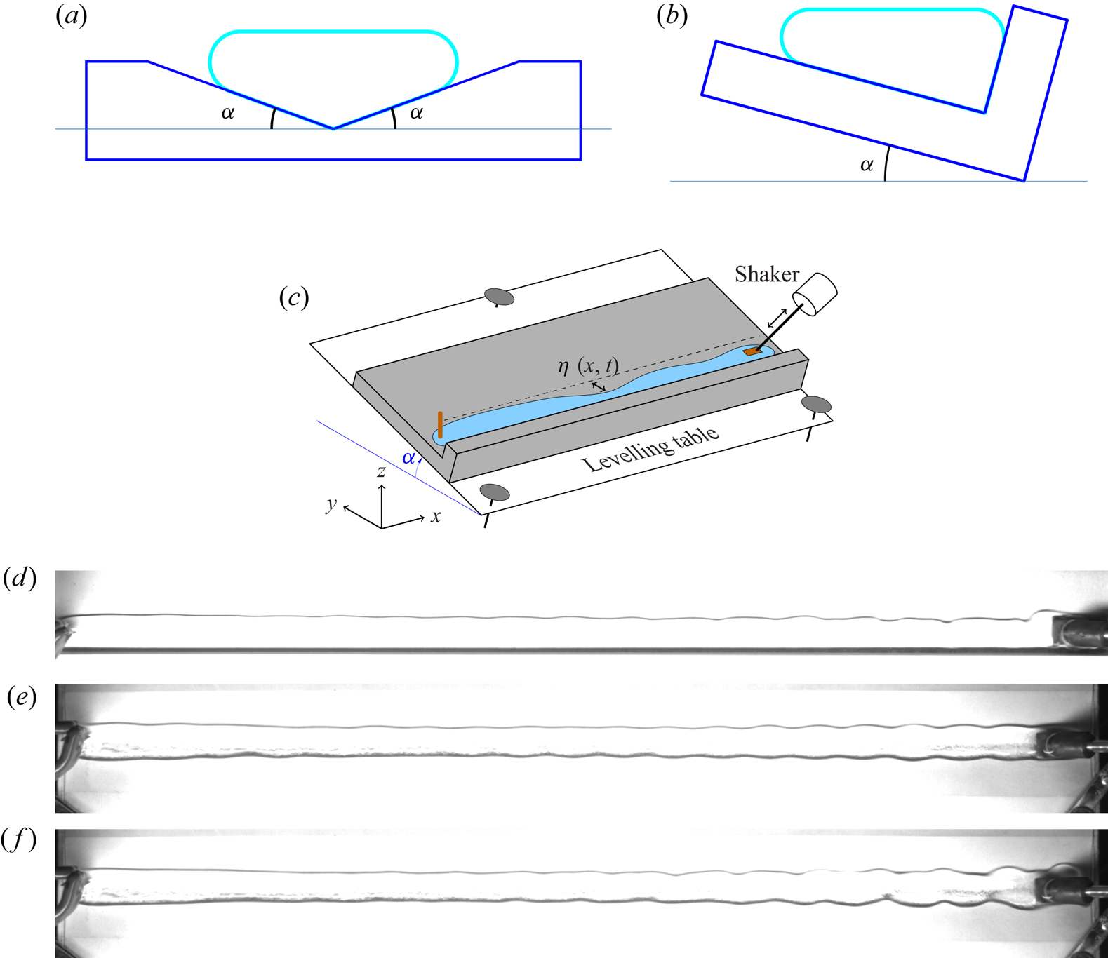
We use the same two different substrates as in Pham et al. (Reference Pham, Perrard and Le Doudic2020). The first one is a symmetrical V-shaped Dural channel with an angle $\alpha =10^{\circ }$. The second one is an L-shaped Dural channel, placed upon a levelling table, so that it can be tilted by an angle $\alpha$, set from $0^{\circ }$ up to $45^{\circ }$ (see the schematics in figure 2a–c). The surface of these substrates is treated using Rust-Oleum NeverWet, so that the wetting conditions can be considered as superhydrophobic (contact angle around $160^{\circ }$; see Gupta, Vaikuntanathan & Siakumar Reference Gupta, Vaikuntanathan and Siakumar2016). Both channels are 50 cm long. On either of them, a controlled volume of distilled water is deposited and stretched from one end to the other end of the channel. If the deposited volume is sufficiently large, such long drops can be pinned at both ends of the channel without breaking up (see Pham et al. Reference Pham, Perrard and Le Doudic2020).

Figure 2.

Geometry of the two different substrate shapes used in our experiments. (a) Cross-section of the V-shaped substrate ($\alpha = 10^{\circ }$). (b) Cross-section of the L-shaped substrate. (c) Schematic of the experimental set-up. Movies are recorded from above. (d–f) Top views of experiments of shaken drops of volume 40 ml. (d) On the non-symmetrical L-shaped substrate tilted by an angle $\alpha =10^{\circ }$. (e) On the symmetrical V-shaped substrate. Varicose modes, i.e. constriction modes, are observed. They are symmetrical in the V-shaped case. In contrast, on the L-shaped substrate, due to the asymmetry, only the constrictions of the interface border located at the gentle sloping side (upper side of the image) are clearly visible. ( f) On the V-shaped symmetrical substrate. The generation of sinuous modes when excited close to their cutoff frequency can be seen.

In order to study the propagation of waves along these drops, we force one end of the drop using a shaker at slowly increasing frequencies from 1 to 20 Hz. Three snapshots are shown as an illustration in figure 2(d–f). The plate connected to the shaker can be seen at the right-hand side of the photographs. The photographs correspond to excited drops of volume equal to 40 ml, deposited on the symmetric V-shaped substrate and the non-symmetrical L-shaped substrate with a tilt angle $\alpha =10^{\circ }$. In the symmetrical case, constriction modes are clearly visible near the shaker; whereas, in the non-symmetrical case, only the deformations of one side of the drop can be captured, as the deformations of the border of the drop at the steepest side of the substrate are too small to be visible. We then naturally focus on the interface located on the smallest slope of the substrate.

The deformation of the interface border is recorded from above using a digital camera (AVT Manta G223) at 50 frames per second. The position of the interface border, $\eta (x,t)$, is numerically reconstructed using an algorithm of contour detection based on the change in the colour gradient, with a 0.03 mm accuracy.

From the camera recordings, we compute the spatio-temporal spectrum $S^{\eta }(k,\omega )$ of the perturbed interface by performing fast Fourier transforms (FFTs) on the difference $\eta(x,t)-\eta_0(x)$, where $\eta_0(x)$ is the shape of the border at rest. The typical spatial resolution is of the order of $0.25$ mm per pixel, and we use a typical image resolution equal to 1700 pixels.

2.2. Experimental results

Several branches can be observed from the obtained spatio-temporal spectra (see figures 3 and 4). We will focus first on the lowest branch, which goes to zero when $k\to 0$ (namely, the varicose branch), then on the other branches (characterised by a low-frequency cutoff at $k=0$), which are related to other modes of wave propagation. The very first upper branch is related to sinuous modes (in the V-shaped case), while the other ones correspond to sloshing modes.

Figure 3.

(a–c) Spatio-temporal spectra $S^{\eta }(k,\omega )$ of the deformation of the border of elongated drops, on a superhydrophobic symmetric V-shaped substrate for three different volumes $V$: (a) $V = 120\ {\rm ml}$, (b) $V = 80$ ml and (c) $V = 35$ ml, at fixed angle $\alpha =10^{\circ }$. The larger the volume, the larger the slope at the origin, that is, the speed of sound. We have superimposed the analytical non-dispersive relation $\omega =c_{{\textit{eff}}}\,k$ (dashed white, with respective values of $c_{{\textit{eff}}}$: (a) $15.9$ cm s$^{-1}$, (b) $13.8$ cm s$^{-1}$ and (c) $9.9$ cm s$^{-1}$) along with the dispersion relation (1.1) with the $\tanh$ function as an ansatz of $\varPsi$ (solid cyan). The agreements are very good. At large volumes (greater than 80 ml), the dispersion relation is not convex; this is the gravity-dominated regime. For smaller volumes (which will correspond to regimes of Bond numbers larger than a critical value), the dispersion relation is purely convex; this is the capillary-dominated regime. The other branches are characterised by a cutoff frequency. They correspond to other modes of propagation (sinuous and sloshing modes). In panel (c) at a volume of water equal to 35 ml, we can clearly distinguish two branches with cutoff frequencies $f_{\textit{sinuous}}\simeq 2.6$ Hz and $f_{\textit{slosh}}\simeq 10$ Hz. (d) Spectrum $S^{W}(k,\omega )$ of $W(x,t)$, the width of the same drop, at $V=35$ ml (see text for its definition), plotted in log–log scale. The sinuous branch with cutoff frequency $f_{\textit{sinuous}}\simeq 2.6$ Hz vanishes; only the varicose mode branch, as well as the upper sloshing branch, remain. For $k\to 0$, $\omega (k)$ scales like $k$ (non-dispersive regime), while for $k\to \infty$, $\omega (k)$ scales like $k^{3/2}$.

Figure 4.

Spatio-temporal spectra of elongated drops, on a superhydrophobic asymmetrical L-shaped substrate for volume equal to 35 ml and four different angles: (a) $\alpha =10^{\circ }$, (b) $\alpha =20^{\circ }$, (c) $\alpha =30^{\circ }$ and (d) $\alpha =40^{\circ }$. We have superimposed the analytical non-dispersive relation $\omega =c_{{\textit{eff}}}\,k$ together with the dispersion relation (1.1) with the $\tanh$ function as an ansatz of $\varPsi$. The larger the angle, the larger the slope, i.e. the greater the propagation speed of long-wavelength varicose modes. We have (a) $c_{{\textit{eff}}} = 12.8$ cm s$^{-1}$, (b) $16.2$ cm s$^{-1}$, (c) $17.9$ cm s$^{-1}$ and (d) $18.7$ cm s$^{-1}$. In this low-volume regime, the varicose branches are convex. No sinuous branch is visible.

We have analytically characterised the long-wave regime ($k\to 0$ limit) of the varicose modes in Pham et al. (Reference Pham, Perrard and Le Doudic2020), with a very good agreement with the experiments. From the value of the deposited volume $V_0$ and the substrate geometry (given by the angle $\alpha$), we were able to deduce the value of the geometric parameter $m$ that sets the section of the drop at rest. Then we deduced the slope at zero of the varicose branch, corresponding to the phase velocity $c_{{\textit{eff}}}$ of the varicose modes. Note that this wedge-shaped geometry corresponds to the ansatz used in Perrard et al. (Reference Perrard, Deike, Duchêne and Pham2015). In this latter work, the authors found a corrective 0.8 factor, because of the curvature of the substrate bottom, which made the actual cross-sectional area lower than that of the ansatz.

We can then deduce the parameter $W_{{\textit{eff}}}=c_{{\textit{eff}}}^{2}/g_{{\textit{eff}}}$ in the dispersion relation (1.1), and we have superimposed the latter onto the spectra using $\varPsi \equiv \tanh$. This functional ansatz will be justified in § 3. Moreover, in order to take into account the short-wave dispersive regime where $\omega ^{2}\sim (\sigma _{{\textit{eff}}}/\rho ) k^{3}$, we have fitted the experimental varicose curve using a fitted value of $\sigma _{{\textit{eff}}}$, typically about $57$ mN m$^{-1}$. As already observed in the case of levitating Leidenfrost cylinders (see Perrard et al. Reference Perrard, Deike, Duchêne and Pham2015), this value is below its expected value ($72$ mN m$^{-1}$ in the superhydrophobic case). This property is due to the non-uniform distribution of curvature of the interface along its section border. This point is thoroughly discussed in § 4 and Appendices A and B. The agreement is very good for both the V-shaped and the L-shaped cases. Note that, in the V-shaped case, the curve loses its convexity, as expected, when the Bond number is below the critical Bond number. This transition between a capillary- and a gravity-dominated regime occurs at a critical volume $V_{{\textit{c}}}\simeq 80$ ml (see discussion in § 4).

Several upper branches $\omega =\omega (k)$, those that do not go to zero at $k\to 0$, are clearly visible in the spectra. In order to characterise the first upper branch, we consider the spectra of the interface border in the V-shaped case. The geometry allows us to capture both the upper $\eta ^{\textit{up}}(x,t)$ and the lower $\eta ^{\textit{lo}}(x,t)$ borders of the interface. The spectrum of $\eta ^{\textit{up}}(x,t)$ is shown in figure 3(c) for a volume $V=35$ ml, whereas we have plotted the spectrum of the difference $W(x,t)=\eta ^{\textit{up}}(x,t)-\eta ^{\textit{lo}}(x,t)$, which corresponds to the spectrum of the drop width (figure 3d). The last is plotted in log–log scale in order to evidence the long-wave regime (for $k\to 0$, where $\omega (k)$ scales like $k$) along with the short-wave regime (for $k\to \infty$, where $\omega (k)$ scales like $k^{3/2}$). The first upper branch has vanished. It corresponds to a motion of the drop of constant section, namely to sinuous modes.

The other upper branches are related to sloshing modes because of the presence of the substrate. The cutoff frequencies of the sinuous and the sloshing modes decrease for increasing values of the deposited volume of liquid. Comparisons with numerical simulations are made in § 3 in the V-shaped case.

In the case of the L-shaped substrate, by inspection of figure 4(a–d), one can tell that, at a fixed volume $V=35$ ml, the cutoff frequencies increase as the angle $\alpha$ increases. A quantitative measurement of these cutoff frequencies along with a comparison with numerical simulations will be discussed in § 3. No sinuous branch is visible.

3.1. Governing equations and classic results

In this section, we present the equations that govern the propagation of surface waves in the $x$-direction, along a channel of given cross-section of water at rest $S_0$, without taking surface tension into account. The flat free interface is denoted $\varGamma _0$ and the solid bottom of the substrate is denoted $\varGamma _1$ (see figure 5a). Let us consider an irrotational, incompressible, inviscid flow. We set $\varPhi (x,y,z)$ as the velocity potential and separate it into $\varPhi (x,y,z,t) = \phi (y,z)\,{\rm e}^{{\rm i}(kx - \omega t)}$. Then the problem to solve is this: Find a non-zero function $\phi (y,z)$ such that there exists $\omega$ that satisfies (see Lamb Reference Lamb1932)

(3.1)\begin{gather} (\varDelta-k^{2}) \phi = 0, \quad \forall (y,z) \in S_0, \end{gather}

(3.2)\begin{gather}\frac{\partial \phi}{\partial n} = 0, \quad \forall (y,z)\in \varGamma_1, \end{gather}

(3.3)\begin{gather}\frac{\partial \phi}{\partial y } = \frac{\omega^{2}}{g} \phi, \quad \forall (y,z)\in \varGamma_0. \end{gather}

This corresponds to a generalised eigenvalue problem. As stated in McIver & McIver (Reference McIver and McIver1993) and Groves (Reference Groves1994), very few analytical solutions of the problem (3.1)–(3.3) can be exhibited. We will present the two standard following ones.

Figure 5.

(a) General notation of the numerical problem. Here $W$ denotes the width of the horizontal free interface $\varGamma _0$; $S_0$ denotes the cross-sectional area of the cylinder at rest; $\varGamma _1$ denotes the solid boundary of the channel; and $H$ denotes the maximum depth of the liquid. (b) Rectangular geometry. (c) Symmetrical square triangle geometry.

3.1.1. Rectangular channel

In the case of a rectangular channel of depth $H$ and width $W$ (see figure 5b), we have a discrete set of dispersion relations, indexed by an integer $N$:

(3.4)\begin{equation} \omega^{2}(k)=g\mu_N(k)\tanh[\mu_N(k)H], \end{equation}

with

(3.5)\begin{equation} \mu_N(k) = \sqrt{\frac{N^{2} {\rm \pi}^{2}}{W^{2}} + k^{2}}. \end{equation}

The case $N=0$ yields the classic dispersion relation

(3.6)\begin{equation} \omega^{2}(k)=gk \tanh kH. \end{equation}

In the limit $kH\to 0$, we have $\omega ^{2}=c_0^{2} k^{2}$ with $c_0^{2}=gH$.

For positive integers $N$, the other branches possess a cutoff frequency $\omega _{{\textit{cut}}}(N)$ that reads

(3.7)\begin{equation} \omega_{{\textit{cut}}}^{2}(N) = g\left[\frac{N{\rm \pi}}{W} \tanh \left(H \frac{N{\rm \pi}}{W}\right)\right]. \end{equation}

For $N=1$ and a depth $H$ much smaller than the width $W$, the first cutoff frequency then reads

(3.8)\begin{equation} \omega_{{\textit{cut}}}(N=1) \underset{H/W\ll 1}{=} \frac{{\rm \pi} \sqrt{gH}}{W}. \end{equation}

3.1.2. Square symmetrical wedge-shaped channel

In the case of a square symmetrical wedge-shaped channel (see figure 5c), exact solutions can be exhibited as well (Lamb Reference Lamb1932; Wehausen & Laitone Reference Wehausen and Laitone1960, p. 551; Groves Reference Groves1994). The first two branches (varicose and first sloshing modes), respectively, satisfy the following dispersion relations:

(3.9)\begin{gather} \omega^{2}=\frac{g}{\sqrt 2} k \tanh \frac{kH}{\sqrt 2}, \end{gather}

(3.10)\begin{gather}\omega^{2}=\frac{g}{\sqrt 2} k \operatorname{cotanh} \frac{kH}{\sqrt 2}. \end{gather}

Rewriting (3.9) as $\omega ^{2}=g_{{\textit{eff}}}\,k \tanh (W_{{\textit{eff}}}\,k)$ yields $g_{{\textit{eff}}}=g\sin \alpha$ with $\alpha = {\rm \pi}/4$. Note that, in the long-wavelength limit, we recover the non-dispersive varicose regime

(3.11)\begin{equation} \omega^{2}\underset{k\to 0}{=}\frac{gH}{2} k^{2}. \end{equation}

Note that (3.11) is valid for any wedge-shaped channel, regardless of the wedge slopes.

The cutoff frequency of the first branch is

(3.12)\begin{equation} \omega_{{\textit{cut}}}(N=1) = \sqrt{\frac{g}{H}}, \end{equation}

and, in order to obtain the upper branches of the dispersion relations, one has to resort to numerical calculations (Groves Reference Groves1994).

3.2. Numerical results

We now turn to the general case of an arbitrary triangular channel section, with angles $\alpha$ and $\beta \geq \alpha$ (see figure 6a). In such a geometry, the substrate is unequivocally characterised by its height $H$ and its angles $\alpha$ and $\beta$. We recall that the relationships between the height $H$, the width $W$ and the cross-sectional area $S$ are given by

(3.13)\begin{gather} W = \frac{\sin(\alpha+\beta)}{\sin\alpha \sin\beta} H, \end{gather}

(3.14)\begin{gather}S = \frac 12 W H = \frac 12 \frac{\sin(\alpha+\beta)}{\sin\alpha \sin\beta} H^{2}=\frac 12 \frac{\sin\alpha \sin\beta}{\sin(\alpha+\beta)}W^{2}, \end{gather}

which yields for our substrates $W = (\cot \alpha )H$ in the V-shaped case and $W = H/{\sin 2\alpha }$ in the L-shaped case. The eigenvalue problem (3.1)–(3.3) depends on six independent quantities: $\alpha ,\ \beta ,\ g,\ \omega ,\ H$ and $k$. The Buckingham ${\rm \pi}$ theorem implies that our system is governed by four independent dimensionless numbers $\alpha ,\ \beta ,\ \varOmega = \omega \sqrt {H/g}$ and $K=kH$. Hence, $H$ sets our length scale and $\sqrt {H/g}$ our time scale.

Figure 6.

(a) Schematic of the geometry: example of a two-dimensional mesh used in numerical simulation (low spatial resolution, here 239 elements). (b,c) Two spectra: (b) V-shaped case and (c) L-shaped case, for an angle $\alpha = 10^{\circ }$. Note that, in the L-shaped case, branches do not converge asymptotically in pairs as in the V-shaped case. (d) Comparison between the classic $\tanh$ function (dashed line) and the actual shape function $\varPsi _{\alpha ,\beta }$ for the V-shaped and the L-shaped cases (solid lines). The two shape functions are almost identical, whereas they differ from the $\tanh$ function at intermediate values of $\xi$.

In order to obtain the dispersion relation of the problem, we resort to numerical computations. To that end, we have discretised the domain into a two-dimensional triangular mesh using the MATLAB/Octave mesh2d mesh generator (Engwirda Reference Engwirda2014). A Lagrange $\mathbb {P}_1$ finite element method is used to solve the problem (3.1)–(3.3), which consists in a generalised eigenvalue problem. The numerical computations yield different branches $\varOmega (K)$. A typical number of 2000–4000 elements is used in order to ensure numerical convergence, depending on the angles $\alpha$ and $\beta$.

The first branch, the one that goes to zero as $k\to 0$, corresponds to the varicose modes. Their dispersion relation reads in physical units

(3.15)\begin{equation} \omega^{2}(k)=(g\sin\alpha) k \varPsi_{\alpha,\beta}\left(\frac{kH}{2\sin\alpha}\right) =(g_{{\textit{eff}}}\,k) \varPsi_{\alpha,\beta}(W_{{\textit{eff}}}\,k),\end{equation}

with the function $\varPsi _{\alpha ,\beta }$, for given angles $\alpha$ and $\beta$, having the following properties:

(3.16)\begin{gather} \varPsi_{\alpha,\beta}(\xi)\underset{\xi\to 0}{\sim} \xi, \end{gather}

(3.17)\begin{gather}\lim_{\xi\to+\infty} \varPsi_{\alpha,\beta}(\xi) = 1, \end{gather}

with $W_{{\textit{eff}}}=H/(2\sin \alpha )$ being the effective width. The boundary conditions (3.16) and (3.17) of the function $\varPsi _{\alpha ,\beta }$ are chosen so that they are the same as those of the $\tanh$ function in the classic cases, as mentioned in § 3.1 (rectangular and square symmetrical triangle), thus allowing direct comparisons. Note that the prefactor $g_{{\textit{eff}}}\,k$ does not depend on $\beta$; it only depends on the smallest angle $\alpha$.

We can deduce the function $\varPsi _{\alpha ,\beta }(\xi )$ by considering the numerical ratio

(3.18)\begin{equation} \varOmega^{2}/[(\sin\alpha)K]=\varPsi_{\alpha,\beta}[K/(2\sin\alpha)]. \end{equation}

This result is depicted in figure 6(d).

From the numerical computations, we obtain the upper branches as well. They are characterised by a cutoff frequency $\omega _{\textit{cut}}(N)$. For different angles $\alpha$ and $\beta$, the first three cutoff frequencies are computed and shown in figure 7(a,b). At fixed angle $\alpha$, the cutoff frequency is an increasing function of the angle $\beta$.

Figure 7.

For a fixed angle $\alpha$ and for different angles $\beta$ (normally $2{\rm \pi} -\alpha >\beta \geq \alpha$, but we will even consider the case $\beta \leq \alpha$) dimensionless values of $\varOmega _{{\textit{cut}}}(N)={\omega _{{\textit{cut}}}(N)}\sqrt {H/g}$, for $N= 1,\ 2$ and $3$, and (a) $\alpha = 15^{\circ }$ and (b) $\alpha = 45^{\circ }$.

More specifically, we have performed the same calculations in the particular cases of V-shaped and L-shaped substrates in order to relate them to our experiments (see figure 8). At fixed depth, for both the V-shaped and L-shaped substrates, the cutoff frequencies $\omega _{\textit{cut}}(N)$ are increasing functions of the angle $\alpha$. In the limit $\alpha \to 0$, the cutoff frequencies decrease linearly towards zero: the less steep the channel, the slower the sloshing motion.

Figure 8.

(a) V-shaped substrate: numerical calculations of the first three dimensionless cutoff frequencies $\varOmega _{{\textit{cut}}}(N) = {\omega _{{\textit{cut}}}(N)} \sqrt {H/g}$ for a given angle $\alpha$. (b) L-shaped substrate: numerical calculations of $\varOmega _{{\textit{cut}}}(N)$ (solid circles), together with a comparison with the experimental measurements of $\omega _{{\textit{cut}}}^{\textit{expe}}(1)$ using different values of $H_{{\textit{eff}}}$ (open squares, see text); in grey, we use $H_{{\textit{eff}}}=2c_{{\textit{eff}}}^{2}/g$, while in red, we use a smaller $H_{{\textit{eff}}}=c_{{\textit{eff}}}^{2}/g$, which yields better agreement.

3.3. Comparison with the experiments

In this section, we compare the cutoff frequencies found in the experimental spectra and the numerical results.

In the case of the V-shaped substrate, the cutoff frequency scales as $\sqrt {g/H}$. The larger the volume, the larger $H$, and therefore the lower the cutoff frequency. For larger volumes of liquid, the measurements of the cutoff frequencies become less accurate. Nevertheless, the larger the volume, the more branches can be distinguished. For instance, four sloshing branches are visible at volume 80 ml in figure 3(a). The value of their cutoff frequencies can be extrapolated at $k=0$: $f_1^{\textit{expe}}\simeq 5.5$ Hz, $f_2^{\textit{expe}}\simeq 9.5$ Hz, $f_3^{\textit{expe}}\simeq 13.3$ Hz and $f_4^{\textit{expe}}\simeq 17.2$ Hz. Their ratios $f_2^{\textit{expe}}/f_1^{\textit{expe}}\simeq 1.73$, $f_3^{\textit{expe}}/f_2^{\textit{expe}}\simeq 1.4$ and $f_4^{\textit{expe}}/f_3^{\textit{expe}}\simeq 1.29$ are in good agreement with the numerical calculations, which yield the following ratios: $f_2^{\textit{num}}/f_1^{\textit{num}}\simeq 1.59$, $f_3^{\textit{num}}/f_2^{\textit{num}} \simeq 1.43$ and $f_4^{\textit{num}}/f_3^{\textit{num}}\simeq 1.26$ (see figure 8a, where the first three frequencies are displayed).

In the case of the L-shaped substrate, we have performed a series of experiments at fixed volume $V=35$ ml with an angle $\alpha$ varying from $5^{\circ }$ to $45^{\circ }$, by $5^{\circ }$ steps. First we must state that, because of the L-shaped geometry, in particular in the low-angle regime, sinuous modes are penalised, for the steepest side of the substrate prevents the border of the interface from moving laterally and keeping its width constant. We have measured the cutoff frequency of the first visible upper branch $\omega ^{\textit{expe}}_{{\textit{cut}}}(1)$.

From the experimental data, the dimensionless quantity $\omega _{{\textit{cut}}}^{\textit{expe}}(1)\sqrt {H_{{\textit{eff}}}/g}$, where $H_{{\textit{eff}}}$ is a length, can be computed and compared to the numerical calculations of $\varOmega _{{\textit{cut}}}(N)$. It is known that, for any triangle of height $H$, we have exactly $c_{{\textit{eff}}}^{2}=gH/2$ (see (3.10) in Pham et al. Reference Pham, Perrard and Le Doudic2020). From the value of $c_{{\textit{eff}}}^{2}$ of our drop, if we consider $H_{{\textit{eff}}}=2 c_{{\textit{eff}}}^{2}/g$, we do not find any agreement between the numerical and the experimental results; the relative error is 40 %. If $H_{{\textit{eff}}}= c_{{\textit{eff}}}^{2}/g$ is chosen instead, the agreement becomes good and the data seem to correspond to the first sloshing branch (see figure 8b). The larger the angle, the larger the cutoff frequency. Determining the exact value of $H_{{\textit{eff}}}$ remains an open question. It can most likely be attributed to the presence of the capillary cap on top of the wedge-shaped volume of water, which has an effect on the experimental value of $\omega ^{\textit{expe}}_{{\textit{cut}}}(1)$, while the sequence of the cutoff frequency ratios may still be described by a sole wedge-shaped cross-section.

4.1. Dispersive effects due to the shape function $\varPsi _{\alpha ,\beta }$

From the numerical calculations presented in § 3, we have evidenced the dispersion relation of the varicose modes propagating along a wedge-shaped channel of angles $\alpha$ and $\beta$. It is given by (3.15) and, because the shape function $\varPsi _{\alpha ,\beta }$ is not a linear function, dispersive effects are intrinsically present. A Taylor expansion of the shape function $\varPsi _{\alpha ,\beta }(\xi )$ at order three in $\xi$ yields the first dispersive correction of the dispersion relation at small wavenumbers$~k$, which reads

(4.2)\begin{equation} \omega^{2} \underset{k\to 0}= g_{{\textit{eff}}}\,k ( W_{{\textit{eff}}}\,k + \tfrac 1 6 \varPsi_{\alpha,\beta}'''(0) W_{{\textit{eff}}}^{3}\kern0.06em k^{3} )+ \mathscr{O}(k^{6}). \end{equation}

This correction is given by $\varPsi _{\alpha ,\beta }'''(0)$. From the numerical calculations, its value can be numerically deduced, insofar as $\varPsi _{\alpha ,\beta }(\xi )\sim \xi$ and $\varPsi _{\alpha ,\beta }$ is an odd function, using the limit

(4.3)\begin{equation} \frac{6}{\xi^{2}}\left(\frac{\varPsi_{\alpha,\beta}(\xi)}{\xi}-1\right)\underset{\xi\to 0}{\longrightarrow}\varPsi_{\alpha,\beta}'''(0). \end{equation}

The results are depicted in figure 9(a,b). The dependence in $\alpha$ and $\beta$ is non-trivial. One can note that, for a fixed value of $\alpha$, $\varPsi _{\alpha ,\beta }'''(0)$ does not vary significantly with $\beta$. This value is of great importance because it sets the value of the critical Bond number at which the dispersion relation starts above (purely convex dispersion relation) or below the non-dispersive dispersion relation (non-convex dispersion relation) (see § 4.3). We will refer to these two regimes as the capillary- and the gravity-dominated regime, respectively.

Figure 9.

(a) Values of $\varPsi _{\alpha ,\beta }'''(0)$ for fixed values of $\alpha$. (b) Same, for fixed values of $\beta$. (c) Particular cases of the V-shaped and L-shaped substrates: dependence of $\varPsi _{\alpha ,\beta }'''(0)$ on the angle $\alpha$. Note that for $\alpha ={\rm \pi} /4=45^{\circ }$, the two situations are the same and we recover $\varPsi _{\alpha ,\beta }'''(0) = \tanh '''(0)=-2$. The curve of the L-shaped substrate has been symmetrised about $\alpha =45^{\circ }$; the values of $\alpha >45^{\circ }$ actually are those of the corresponding angle $\beta =90^{\circ }-\alpha$. In all cases, the value of $|\varPsi _{\alpha ,\beta }'''(0)|/6$ yields the critical Bond number (see § 4.3).

In figure 9(c) are displayed the values of $\varPsi _{\alpha ,\beta }'''(0)$ in the particular cases of the V-shaped and the L-shaped substrates. At angle $\alpha ={\rm \pi} /4$, we recover the value $\tanh '''(0) = -2$, whereas for $\alpha \to 0$, we have $\varPsi _{\alpha ,\beta }'''(0) \to -1$. In the V-shaped case, when $\alpha \to {\rm \pi}/2$, we have $\varPsi _{\alpha ,\beta }'''(0) \to -3$.

4.2. An analytical estimation of $\sigma _{{\textit{eff}}}$

We propose an estimation of $\sigma _{{\textit{eff}}}$ as a cross-sectional averaging of the hydrostatic pressure field, by taking into account the non-uniform profile of curvature of the interface along the transverse section of it, due to the presence of varicose modes. In short, we go one step further than the non-dispersive calculation of Pham et al. (Reference Pham, Perrard and Le Doudic2020) and calculate the $k^{4}$ contribution in the framework of the Saint-Venant equations. Owing to the length of the derivations, their technical details are deferred to Appendix B, where we first analytically compute the curvature of the interface of the varicose modes using an adiabatic hypothesis on the sections. We then perform an estimation of the averaged pressure gradient that yields $\sigma _{{\textit{eff}}}$, through a toy model. This toy model is motivated by a few statements on how dispersive effects due to surface tension can be taken into account within the Saint-Venant formalism we used to study the non-dispersive regime of our sessile cylinders (Pham et al. Reference Pham, Perrard and Le Doudic2020). These statements are made in Appendix A.

The main result of this study is that, because of the non-flat interface, the perturbative curvature profile along the interface when varicose perturbations are present is non-trivial. At low angle $\alpha$, the curvature is dominant at the drop tip, while at steep angle $\alpha$, the maximum of the curvature is reached about the top of the drop. The uneven distribution of curvature leads to an effective reduced surface tension of about 57 mN m$^{-1}$ observed in our experiments, in both the V-shaped and the L-shaped substrates. The comparisons with the experiments are summarised in tables 1 and 2.

Table 1.

Case of the V-shaped substrate. Experimental values of $\sigma _{{\textit{eff}}}$ found by fitting the spectra, using (1.1), for different volumes $V$ and comparison with the toy model. The agreement is fair, with a relative error of 15 %.

Table 2.

Case of the L-shaped substrate. Comparison of the values of $\sigma _{{\textit{eff}}}$ between experiments and toy model. The agreement is good, with an error of less than 10 %.

In the case of our V-shaped geometry, at a low angle $\alpha = 10^{\circ }$, the fitting of the value of $\sigma _{{\textit{eff}}}$ does not show much dependence on the volume, and nor do the values yielded by the toy model, which undershoots the experimental value with an error of 15 %. In the case of our L-shaped substrate, the experimental values do not show any obvious dependence on the angle $\alpha$, while the toy model we used shows a small decrease in the values of $\sigma _{{\textit{eff}}}$ with increasing angles $\alpha$. In any case, we obtain a better agreement than in the V-shaped case. The error is of 10 % with the experimental data.

4.3. Effective Bond number and critical value

From the general dispersion relation (1.1) and the Taylor expansion of $\varPsi (\xi )$ at order three, we get, at order $k^{4}$,

(4.4)\begin{equation} \omega^{2} = c_{{\textit{eff}}}^{2}\kern0.05em k^{2} [1 + (\textit{Bo}_{{\textit{eff}}} - \textit{Bo}_{{\textit{c}}})k^{2}W_{{\textit{eff}}}^{2}]+ \mathscr{O}(k^{6}), \end{equation}

with the effective Bond number and the critical Bond number defined as

(4.5a,b)\begin{equation} \textit{Bo}_{{\textit{eff}}} = \frac{\sigma_{{\textit{eff}}}}{\rho g_{{\textit{eff}}}W_{{\textit{eff}}}^{2}},\quad \textit{Bo}_{{\textit{c}}} = \frac{|\varPsi'''(0)|}{6}. \end{equation}

In the V-shaped and L-shaped cases, both quantities depend strongly on the angle $\alpha$. The difference $\textit{Bo}_{{\textit{eff}}} - \textit{Bo}_{{\textit{c}}}$, as can be seen in (4.4), ensures whether the dispersion relation is purely convex (namely, is always above its tangent), yielding the capillary-dominated regime, or starts like a concave curve in the neighbourhood of the origin (the dispersion relation curve starts under the line $\omega =c_{{\textit{eff}}}\,k$). In both cases, the shape of the curve is convex at large wavenumbers $k$ ($\omega \sim \sqrt {\sigma _{{\textit{eff}}}/\rho }k^{3/2}$). For a given substrate of given angle $\alpha$, be it an L-shaped or a V-shaped substrate, the larger the volume of water, the larger the effective width $W_{{\textit{eff}}}$ and the smaller the effective Bond number $\textit{Bo}_{{\textit{eff}}}$. Conversely, because of the presence of $g_{{\textit{eff}}}=g\sin \alpha$, $\textit{Bo}_{{\textit{eff}}}$ can reach large numbers when the volume is small (yet larger than the Plateau–Rayleigh threshold).

As can be seen in figure 9(c), the value of $\varPsi '''(0)$ ranges from $-1$ at vanishing $\alpha$, to $-2$ at $\alpha ={\rm \pi} /4$ for a V-shaped substrate, and down to $-3$ for $\alpha$ approaching ${\rm \pi} /2$ when ignoring the capillary cap. These results are valid in the absence of surface tension, or considering that the interface remains horizontal. Now, let us compare the previous results with the experimental results of § 2 in terms of effective Bond number $\textit{Bo}_{{\textit{eff}}}$.

In the V-shaped case with no surface tension, we have $\alpha =10^{\circ }$, $\varPsi _{\textit{num}}'''(0)\simeq -1.061$, so that $\textit{Bo}_{{\textit{c}}}\simeq 1/6\simeq 0.167$. The value of the effective surface tension $\sigma _{{\textit{eff}}}$ is given by fitting the experimental spectra (see table 1). For a volume $V=35$ ml, we find $\textit{Bo}_{{\textit{eff}}}\simeq 1.00$, whereas for a larger volume $V=80$ ml, we find $\textit{Bo}_{{\textit{eff}}}\simeq 0.274$. At volumes less than $V=80$ ml, the dispersion relation curve remains convex and we can note that the curve is linear within a larger range of small $k$ as the volume increases. It seems that the transition occurs in the vicinity of the volume $V=80$ ml (see figure 3). Therefore, from our experiments, we can perform the estimation $\textit{Bo}_{{\textit{c}}}\simeq 0.274$, so that $\varPsi _{\textit{expe}}'''(0)\simeq -6\times 0.274\simeq -1.644$. This result departs from the case without surface tension because of the presence of the capillary cap on top of the triangular wedge.

5.1. Linear part of the Korteweg–de Vries equation

We will start with the following statement: if we consider the first dispersive contribution of the general dispersion relation (1.1), we obtain (4.4), which corresponds to a wave equation that reads

(5.1)\begin{equation} \eta_{tt}-c_{{\textit{eff}}}^{2}[\eta_{xx}+W_{{\textit{eff}}}^{2}(\textit{Bo}_{{\textit{c}}}-\textit{Bo}_{{\textit{eff}}})\eta_{xxxx}] = 0. \end{equation}

The linear part of the KdV equation (1.2) reads

(5.2)\begin{equation} \eta_{t}+c_{{\textit{eff}}}[\eta_{x}+\tfrac 1 2 W_{{\textit{eff}}}^{2}(\textit{Bo}_{{\textit{c}}}-\textit{Bo}_{{\textit{eff}}})\eta_{xxx}] = 0, \end{equation}

and this wave equation corresponds to travelling waves in the right direction.

5.2. Saint-Venant equations as nonlinear acoustics equations

In order to obtain the nonlinear contribution in (1.2), we will use the Saint-Venant equations previously used in Part 1 of this work (Pham et al. Reference Pham, Perrard and Le Doudic2020) and treat them as nonlinear acoustics equations. The aim is to eliminate the averaged speed in the Saint-Venant equations and obtain a nonlinear wave equation in the section variable only. The details of the derivation are deferred to Appendix A.3. They follow a calculation due to Earnshaw (Reference Earnshaw1860), as presented by Whitham (Reference Whitham1999, § 6.9). In this subsection, we will disregard the surface tension effects and suppose that the transverse section of liquid has a flat horizontal free interface.

We start from the Saint-Venant equations

(5.3)\begin{gather} \partial_t S + \partial_x{(S\bar u)} = 0, \end{gather}

(5.4)\begin{gather}\partial_t \bar u + \bar u \partial_x \bar u + \frac 1\rho \langle\partial_x P\rangle =0, \end{gather}

for a transverse section of the liquid $S(x,t)$, a section-averaged velocity in the $x$-direction $\bar u(x,t)$ and a section-averaged hydrostatic pressure gradient $\langle \partial _x P(x,t)\rangle$ (see Pham et al. Reference Pham, Perrard and Le Doudic2020). In the context of a section with a horizontal free interface, the section-averaged pressure gradient reads $\langle \partial _x P\rangle = \rho g \partial _x H$, where $H(x,t)$ denotes the vertical position of the free interface. As we want eventually to obtain an equation in the variable $S$ only, we first write $H$ as a function of the cross-sectional area $S$ and perform the symbolic substitution $(1/\rho ) \langle \partial _x P \rangle \equiv ({1}/{S}) \partial _x \varPi (S)$. The Saint-Venant equations then become

(5.5)\begin{gather} \partial_t S + \partial_x{(S\bar u)} = 0, \end{gather}

(5.6)\begin{gather}\partial_t \bar u + \bar u \partial_x \bar u + \frac{1}{S} \partial_x \varPi(S) =0, \end{gather}

which are equivalent to the one-dimensional compressible Euler equations governing the dynamics of a compressible isentropic gas of density $\varrho (x,t)$, velocity $\bar u(x,t)$ and pressure field $\varPi (x,t)$.

In the case of a polytropic gas, namely a system that has an equation of state that reads $\varPi (S) = \kappa S^{\gamma }$, and in the case of a wave travelling in the right direction, $\bar u$ can be eliminated in (5.5) and we obtain the nonlinear wave equation

(5.7)\begin{equation} \partial_t S +c_0\left( 1+ \frac{\gamma+1}{2} \frac{S-S_0}{S_0}\right)\partial_x S = 0.\end{equation}

In the case of a rectangular section, we have $\gamma =2$. In the case of a triangular section, we have $\gamma =3/2$. Note that, if the nonlinear terms are neglected, we recover the non-dispersive linear regime.

The linear waves in the variable $S(x,t)$ actually follow the dispersion relation (5.2) at first dispersive order. Taking into account the first correction both in nonlinearity and in dispersion thus yields the following KdV equation:

(5.8)\begin{equation} \partial_t S +c_{{\textit{eff}}}\left[ \partial_x S + \frac{\gamma+1}{2} \frac{S-S_0}{S_0}\partial_x S + \frac 12 W_{{\textit{eff}}}^{2} (\textit{Bo}_{{\textit{c}}} -\textit{Bo}_{{\textit{eff}}})\partial_{xxx}S\right]= 0. \end{equation}

For a rectangular channel of width $W$ and depth at rest $H_0$, we have $S(x,t)=W H(x,t)$, $c_{{\textit{eff}}}=\sqrt {gH_0}$ and $\gamma =2$. Moreover, $\varPsi (\xi )=\tanh (\xi )$ so that $\varPsi '''(0) = -2$ and $\textit{Bo}_{{\textit{c}}} = 1/3$. By using $\eta =H(x,t)-H_0$ as the variable, the standard KdV equation is recovered, which reads

(5.9)\begin{equation} \partial_t \eta +\sqrt{gH_0}\left[ \partial_x \eta + \frac{3}{2} \frac{\eta}{H_0}\partial_x \eta + \frac 12 H_0^{2} \left(\frac 13 -\frac{\sigma}{\rho g H_0^{2}}\right)\partial_{xxx}\eta\right]= 0. \end{equation}

In the case of a wedge-shaped channel with a flat interface (surface tension is taken into account but not the capillary cap) and of depth $H_0$, we have $c_{{\textit{eff}}}=\sqrt {gH_0/2}$ and $W_{{\textit{eff}}} = H_0/(2\sin \alpha )$. The variations of the cross-sectional area are related to the displacement of the border of the interface, hence to the variations of the width of the interface, which will be denoted $W$. The cross-sectional area $S$ is proportional to $W^{2}$ so that the ratio $(S-S_0)/S_0$ becomes $2(W-W_0)/W_0$ with $W_0 = \sin (\alpha +\beta )/(\sin \alpha \sin \beta ) H_0=2[\sin (\alpha +\beta )/{\sin {\beta }}]W_{{\textit{eff}}}$ (see (3.14)). The KdV equation for a general triangle now reads, in terms of variable $\eta =W-W_0$, with $W_0$ the width at rest:

(5.10)\begin{equation} \partial_t \eta +c_{{\textit{eff}}}\left[ \partial_x \eta + \left(\frac{5}{4} \frac{\sin\beta}{\sin(\alpha+\beta)}\right) \frac{\eta}{W_{{\textit{eff}}}}\partial_x \eta + \frac 12 W_{{\textit{eff}}}^{2} (\textit{Bo}_{{\textit{c}}} -\textit{Bo}_{{\textit{eff}}}) \partial_{xxx}\eta \right]= 0, \end{equation}

for angles $\alpha <\beta$, with $\textit{Bo}_{{\textit{c}}} = |\varPsi _{\alpha ,\beta }'''(0)|/6$ and $\textit{Bo}_{\textit{eff}}=\sigma/(\rho g_{\textit{eff}} W_{\textit{eff}}^2)$.

In the L-shaped case ($\alpha ={\rm \pi} /2-\beta$) and for small values of $\alpha$, the prefactor $\sin \beta /{\sin (\alpha +\beta )}$ is close to $1$ and can be ignored in this limit. We then have the approximation $5/4\times \sin \beta /{\sin (\alpha +\beta )}\simeq 5/4$.

In contrast, in the V-shaped case ($\alpha =\beta$) and for a small angle$~\alpha$, the sinusoidal prefactors add a factor $1/2$ and we have $5/4\times \sin \beta /{\sin (\alpha +\beta )}\simeq 5/8$.

In our experimental set-up, which will consist of an L-shaped triangle with a capillary cap on top, the equation of state is no longer that of a polytropic gas, but rather that of a barotropic gas. In this case, $\varPi (S)$ is no longer a power law. The nonlinear wave equation can be formally derived using the expression of $\varPi (S)$, which could be computed after tedious calculations. Instead of doing so, we assume that the geometrical ansatz of the cylinder cross-section as a triangle of angle $\alpha$ and $\beta$ (hence a polytropic exponent $\gamma = 3/2$) is relevant to yield the nonlinear term in the nonlinear wave equation, so that the KdV equation now reads in the variable $\eta =W-\Delta Y_{\textit{max}}$, where $\Delta Y_{\textit{max}}$ is the width at rest:

(5.11)\begin{equation} \partial_t \eta +c_{{\textit{eff}}}\left[\partial_x \eta + \left(\frac{5}{2} \frac{W_{{\textit{eff}}}}{\Delta Y_{\textit{max}}}\right) \frac{\eta}{W_{{\textit{eff}}}}\partial_x \eta + \frac 12 W_{{\textit{eff}}}^{2} (\textit{Bo}_{{\textit{c}}} -\textit{Bo}_{{\textit{eff}}}) \partial_{xxx}\eta \right]= 0, \end{equation}

with $W_{{\textit{eff}}} = c_{{\textit{eff}}}^{2}/g_{{\textit{eff}}}$, $\textit{Bo}_{{\textit{c}}}$ and $\textit{Bo}_{{\textit{eff}}}$ are given by (4.5a,b), and the prefactor $\nu _1$ in front of the nonlinear term here is

(5.12)\begin{equation} \nu_1 = \frac 52 \frac{W_{{\textit{eff}}}}{\Delta Y_{\textit{max}}}.\end{equation}

5.3. Experimental results

For a KdV equation of the form

(5.13)\begin{equation} \partial_t \eta +c_{{\textit{eff}}}\left[\partial_x \eta + \frac{\nu_1}{W_{{\textit{eff}}}} {\eta}\partial_x \eta + \frac 12 {W_{{\textit{eff}}}}^{2} (\textit{Bo}_{{\textit{c}}} -\textit{Bo}_{{\textit{eff}}}) \partial_{xxx}\eta\right]= 0, \end{equation}

the one-soliton solution reads

(5.14)\begin{equation} \eta(x,t) = A_0 \operatorname{sech}^{2}\left(\frac{x-ct}{\varDelta}\right), \end{equation}

with the following relationship between speed $c$, amplitude $A_0$ and width $\varDelta$:

(5.15)\begin{gather} \frac{c}{c_{{\textit{eff}}}} = 1 + \frac{\nu_1 A_0}{3 W_{{\textit{eff}}}}, \end{gather}

(5.16)\begin{gather}\frac{\varDelta}{W_{{\textit{eff}}}} = \sqrt{2\frac{\textit{Bo}_{{\textit{c}}}-\textit{Bo}_{{\textit{eff}}}}{{c}/{c_{{\textit{eff}}}}-1}}. \end{gather}

In our experiments, we will study the propagation of large negative amplitude waves and see if the relationship (5.15) is satisfied with $\nu _1$ given by (5.12). To that end, we will consider the L-shaped substrate, tilted by a small angle $\alpha =2^{\circ }, 3^{\circ }$ or $4^{\circ }$. We will use a volume of water $V=40$ ml, which is sufficiently small for the effective Bond number to be large compared to the value of critical Bond number, which lies somewhere in between $1/3$ and $1/6$ (see§ 4.3).

In order to generate a large amplitude soliton, we use a micro-pipette that injects a small jet of water inside the sessile liquid cylinder. Because of the jet, a depression is locally created that strongly disturbs the interface (see figure 10a and the supplementary movie available at https://doi.org/10.1017/jfm.2021.502). A train of fast waves and a hump of water are ejected and travel to the other end of the drop. Eventually, a deep depression solitary wave emerges, propagating at a speed $c$ slower than the speed of the non-dispersive waves $c_{{\textit{eff}}}$. Note that, contrary to their Leidenfrost counterpart, because of the dissipation at the contact line, these depression waves damp in a shorter distance about half of the drop.

Figure 10.

(a) Snapshots of the propagation of a KdV soliton. The deposited volume is equal to 40 ml and the angle $\alpha$ is equal to $2^{\circ }$. After a strong perturbation of the surface at the tip of the cylinder, waves propagate ahead of a solitary depression that emerges (see arrows) and propagates at a speed $c$ lower than $c_{{\textit{eff}}}$, the propagation speed of the long-wavelength waves. Eventually, it vanishes. (b) Renormalised propagation speed $c/c_{{\textit{eff}}}$ versus renormalised amplitude $A_0/(3W_{{\textit{eff}}})$. The region $c/c_{{\textit{eff}}}>1$ corresponds to the supersonic soliton regime (namely, the gravity-dominated regime where elevation solitons exist), whereas the region $c/c_{{\textit{eff}}}<1$ corresponds to the subsonic soliton regime (namely, the capillary-dominated regime where depression solitons exist). The data points (SH, for three different angles $\alpha$) seem to follow a straight line of slope $\nu _1\simeq 2$. As a comparison, we have added the experimental data in mercury from Falcon et al. (Reference Falcon, Laroche and Fauve2002) (in grey, following the standard slope $\nu _1=3/2$, each symbol representing a given depth of mercury) along with those obtained by Perrard et al. (Reference Perrard, Deike, Duchêne and Pham2015) in Leidenfrost (open symbols, following a slope $\nu _1^{\textit{expe}}\simeq 3$).

We measure the propagation speed $c$ of this solitary wave as well as its negative amplitude $A_0$. The results are shown in figure 10(b), where the dimensionless ratio $c/c_{{\textit{eff}}}$ is measured with respect to the dimensionless ratio $A_0/3W_{{\textit{eff}}}$. In this plot, we have added the results found by Falcon et al. (Reference Falcon, Laroche and Fauve2002) in experiments performed in mercury; they follow a line of slope $\nu _1=3/2$ in accordance with the rectangular geometry of the tank they use. The measurements in the Leidenfrost case are plotted as well, and they follow a line of slope $\nu _1^{\textit{expe}}\simeq 3$ (Perrard et al. Reference Perrard, Deike, Duchêne and Pham2015).

At volume $V=40$ ml and length $L=50$ cm, the cross-sectional area is $S_{{\textit{tot}}}=V/L=80$ mm$^{2}$; the value of the geometric parameter $m$ yielding the analytical shape of the drop section can then be analytically deduced, as well as the values of the width of the drop $\Delta Y_{\textit{max}}$ and the effective width $W_{{\textit{eff}}}=c_{{\textit{eff}}}^{2}/g_{{\textit{eff}}}$ (see (3.44), (2.20) and (3.47), respectively, in Pham et al. Reference Pham, Perrard and Le Doudic2020). At angles $\alpha =2^{\circ }, 3^{\circ }$ and $4^{\circ }$, the prefactor $\nu _1$ given by (5.12) is then respectively equal to 2.1, 2.03 and 1.99, which are very close to 2. In order to test this prediction, we have plotted the line of slope $\nu _1=2$. From the experimental data points obtained with our superhydrophobic substrate (SH), the most significant points are those with the largest amplitudes and the lowest speeds, since they are the easiest ones to characterise. Those points seem to follow a slope $\nu _1^{\textit{expe}}$ slightly larger than $2$, which is in reasonable agreement with our prediction $\nu _1=2$.

5.4. Korteweg–de Vries solitons in Plateau borders

The method we have presented to derive the KdV equation is generic and it can be applied to other free-interface systems with a cylinder-type geometry. As an illustration of the generality of the method, we will consider the case of Plateau borders, along which the observation of the propagation of depression solitary waves has been reported in experiments using soap films (Argentina et al. Reference Argentina, Cohen, Bouret, Fraysse and Raufaste2015; Bouret et al. Reference Bouret, Cohen, Fraysse, Argentina and Raufaste2016).

A Plateau border is a cylinder of liquid that corresponds to a geometric region bounded by three tangent circles of radius $R(x,t)$. The latter corresponds to the radius of curvature of the cylinder at the coordinate $x$ and time $t$ (see figure 11). The section of a Plateau border of radius of curvature $R$ is given by

(5.17)\begin{equation} S(R)=\left(\sqrt 3 -\frac{\rm \pi}{2}\right)R^{2}. \end{equation}

Let $C$ be one of the three centres of curvature. The distance from the origin to this centre$~C$ is

(5.18)\begin{equation} OC(R) = \frac{R}{2\sqrt{3}}+R\frac{\sqrt 3}{2}=\frac{2}{\sqrt{3}} R. \end{equation}

The distance from the origin to the interface is

(5.19)\begin{equation} Ox_i(R) = |OC(R)|-R = \left(\frac{2}{\sqrt{3}}-1\right) R. \end{equation}

Using the Laplace law, we can then deduce the pressure term, which reads

(5.20)\begin{equation} P(x,t) ={+}\sigma\left[-\frac{1}{R(x,t)} - \left(\frac{2}{\sqrt 3} -1\right)\partial_{xx}R(x,t) \right]. \end{equation}

It is uniform in the section so that we can apply the Saint-Venant formalism. After setting $R=R_0\{1+\varepsilon \exp [{\rm i} (kx-\omega t)]\}$ and $\bar u=\varepsilon u_0\exp [{\rm i} (kx-\omega t)]$, (5.3) and (5.4), at order one in $\varepsilon$, yield the dispersion relation

(5.21)\begin{equation} \omega^{2}=\frac{\sigma}{2\rho R_0}k^{2}\left[ 1+\left(\frac{2}{\sqrt 3}-1\right)R_0^{2} k^{2} \right] \end{equation}

after elimination of $u_0$ and $\varepsilon$.

Figure 11.

Transverse section of a Plateau border of radius of curvature $R$, centred at the origin $O$. Its boundaries are defined as three tangent circle arcs (in blue); and $x_i$ denotes the distance from the centre to the interface. The length $|Cx_i|$ is the radius of curvature $R$ of the Plateau border, and $C$ is the centre of curvature of one of the three interfaces. The Plateau border is circumscribed in a circle of radius $R/\sqrt {3}$, centred at the origin.

It would be interesting to validate this theoretical dispersion relation experimentally. To our knowledge, the dispersion relations of waves along a Plateau border studied so far were related to the sinuous modes (Kosgodagan Acharige, Elias & Derec Reference Kosgodagan Acharige, Elias and Derec2014) and not to the varicose modes.

From the nonlinear acoustics analogy (see Appendix A.3), we can deduce the following equation of state:

(5.22)\begin{equation} \varPi(S) = \frac\sigma\rho \left(\sqrt 3 - \frac{\rm \pi}{2}\right)^{1/2} S^{1/2}, \end{equation}

which corresponds to a polytropic gas, with exponent $\gamma =1/2$. The dispersion relation for linear dispersive waves travelling to the right reads

(5.23)\begin{equation} \omega = c_0 k \left[1+\left(\frac 1{\sqrt{3}}-\frac 12\right)R_0^{2}k^{2}\right], \end{equation}

with $c_0=\sqrt {\sigma /(2\rho R_0)}$. The KdV equation in the $S$ variable can then be derived from (5.8) as

(5.24)\begin{equation} \partial_t S + c_0\left[\partial_x S + \frac {3}{4} \frac{S-S_0}{S_0}\partial_x S - \frac{1}{2}R_0^{2}\left(\frac{2}{\sqrt{3}}-1\right)\partial_{xxx}S\right] = 0. \end{equation}

The KdV equation in the width variable $r$ ($R=R_0+r$) then reads

(5.25)\begin{equation} \partial_t r + c_0 \left[\partial_x r + \frac 3{2R_0} r \partial_x r - \frac{1}{2} R_0^{2} \left(\frac{2}{\sqrt 3} -1\right)\partial_{xxx}r\right] =0. \end{equation}

We then have a soliton solution (5.14) that reads, for $\nu _1=3/2$ and $v=c/c_{{\textit{eff}}}$:

(5.26)\begin{equation} r(x,t) = 2(v-1) R_0 \operatorname{sech}^{2} \frac{x-v c_0 t}{\sqrt{\dfrac{2(2/\sqrt{3}-1)}{1-v}}R_0}\equiv A_0 \operatorname{sech}^{2} \frac{x-v c_0 t}{ \dfrac{2\sqrt\beta}{\sqrt{1-v}}R_0 }. \end{equation}

Experimentally, Bouret et al. (Reference Bouret, Cohen, Fraysse, Argentina and Raufaste2016) found $2\sqrt {\beta _{\textit{expe}}}\simeq 0.4$, whereas we have $2\sqrt {\beta }\equiv \sqrt {2 (2/\sqrt {3} -1)}\simeq 0.56$, which yields a relative error of $40$ %, improving the model used by Argentina et al. (Reference Argentina, Cohen, Bouret, Fraysse and Raufaste2015), who found $2\sqrt \beta =2\sqrt {(2\sqrt 3-{\rm \pi} )/{\rm \pi} }\simeq 0.64$, namely a relative error of $60$ %.