1 Introduction
In the midlatitude troposphere, dynamic low- and high-pressure systems and the large-scale polar jet, a narrow band of high wind speeds in the upper troposphere, develop due to the lateral temperature gradient between the polar region and the equatorial region and form due to midlatitude baroclinic instability. The meandering jet pattern and the embedded cyclonic and anticyclonic pressure systems transport heat and momentum from the tropical to the polar region.
The tropospheric jet is linked with the occurrence of atmospheric inertia–gravity waves (hereafter IGWs for short). O’Sullivan & Dunkerton (Reference O’Sullivan and Dunkerton1995) found that nearly balanced baroclinic life cycles could lead to spontaneous emission of IGWs at the jet exit region. This hypothesis was confirmed later (Plougonven & Snyder Reference Plougonven and Snyder2005, Reference Plougonven and Snyder2007; Viùdez & Dritschel Reference Viùdez and Dritschel2006). Field measurements (Plougonven, Teitelbaum & Zeitlin Reference Plougonven, Teitelbaum and Zeitlin2003) reveal that two distinct regions are responsible for intense emission of IGWs, namely, first, the region of the maximum wind speed within the jet and, second, the region of the strongest curvature of the jet. While Plougonven et al. suggested that geostrophic adjustment leads to the emission of IGWs, Zhang (Reference Zhang2004), studying the emission of IGWs from the tropospheric jet in a numerical experiment, supposed that IGWs are emitted from flow imbalance. Later, Vanneste (Reference Vanneste2013) reported that the evolution of well-balanced flows would lead to the emission of IGWs through spontaneous imbalance, especially in baroclinic life cycles. This is due to the fact that locally large Rossby numbers can be found in localized atmospheric features like in fronts, from which IGWs can be emitted even if the flow is balanced on large scales.
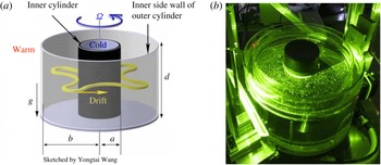
(a) Sketch of the research cavity with a baroclinic wave of dominant azimuthal wavenumber
 $m=4$
, courtesy of Yongtai Wang. (b) Photo of the differentially heated rotating annulus laboratory experiment. The cooled inner cylinder and the two outer cylinders heated in between can be seen. The experiment has a free top surface and a flat bottom. Particle motion in a layer close to the surface has been made visible by a green laser plane.

Quite recently, it was realized that a thermally driven rotating annulus is a suitable testbed for studies on spontaneous imbalance of baroclinic jets; see Williams, Haine & Read (Reference Williams, Haine and Read2008), Flór, Scolan & Gula (Reference Flór, Scolan and Gula2011), Borchert, Achatz & Fruman (Reference Borchert, Achatz and Fruman2014), Vincze et al. (Reference Vincze, Borcia, Harlander and Le Gal2016) and Hien et al. (Reference Hien, Rolland, Borchert, Schoon, Zülicke and Achatz2018). Hien et al. (Reference Hien, Rolland, Borchert, Schoon, Zülicke and Achatz2018) pointed out that for the annulus flow, only some part of the gravity waves seems to result from spontaneous emission. A residual part comes from other sources. To correctly interpret experimental and numerical annulus results on spontaneous imbalance, it is hence of importance to study boundary layer instabilities and to find out whether these instabilities can radiate gravity waves into the region of the baroclinic jet. This is the purpose of the present investigation.
The thermally driven rotating annulus, figure 1, is a laboratory-scale set-up for studying midlatitude atmospheric flows, which are driven by the baroclinicity of the flow state by analogy with atmospheric flows. The set-up generally consists of a cylindrical gap; the bounding walls rotate uniformly around the vertical axis of symmetry with frequency
 $\unicode[STIX]{x1D6FA}$
. The lateral temperature gradient,
 $\unicode[STIX]{x1D6E5}$
, is set by cooling the inner sidewall and heating the outer one, and the cooled inner sidewall then reflects the Earth’s polar region and the heated outer sidewall its equatorial region. The research cavity represents the midlatitudes, where a vertically and horizontally sheared mean flow is generated due to the lateral temperature gradient and the rotation of the annulus. The flow regimes are mainly determined by
 $\unicode[STIX]{x1D6FA}$
and
 $\unicode[STIX]{x1D6E5}$
, and their general characteristics are only weakly dependent on material properties of the liquid (Fein & Pfeffer Reference Fein and Pfeffer1976). However, it should be noted that studies with air as working fluid show somewhat different characteristics of the large-scale flows (Randriamampianina et al.
Reference Randriamampianina, Früh, Read and Maubert2006; Castrejón-Pita & Read Reference Castrejón-Pita and Read2007; Read et al.
Reference Read, Maubert, Randriamampianina and Früh2008).
Using non-dimensional parameters,
 $\unicode[STIX]{x1D6FA}$
and
 $\unicode[STIX]{x1D6E5}$
are typically captured by the Taylor number,
 $Ta$
, and the thermal Rossby number,
 $Ro$
. Both
 $Ta$
and
 $Ro$
include the geometric parameters of the research cavity, specifically its aspect ratio,
 $\unicode[STIX]{x1D6E4}=d/(b-a)$
, with
 $d$
as the fluid depth and
 $(b-a)$
as the gap width. The radius ratio,
 $\unicode[STIX]{x1D702}$
, is given by
 $\unicode[STIX]{x1D702}=a/b$
, with
 $a$
as the inner radius and
 $b$
as the outer radius of the gap. The material properties of the working fluid are defined by the Prandtl number,
 $Pr$
. The three parameters
 $Ta$
,
 $Ro$
and
 $Pr$
read as
 $$\begin{eqnarray}Ta=\frac{4\unicode[STIX]{x1D6FA}^{2}(b-a)^{5}}{\unicode[STIX]{x1D708}^{2}d},\quad Ro=\frac{\unicode[STIX]{x1D6FC}\unicode[STIX]{x0394}gd}{\unicode[STIX]{x1D6FA}^{2}(b-a)^{2}},\quad Pr=\frac{\unicode[STIX]{x1D708}}{\unicode[STIX]{x1D705}},\end{eqnarray}$$
with
 $\unicode[STIX]{x1D6FC}$
as the volumetric expansion coefficient of the fluid,
 $\unicode[STIX]{x1D708}$
as the kinematic viscosity,
 $\unicode[STIX]{x1D705}$
as the thermal diffusivity and
 $g$
as the acceleration due to gravity. The Taylor number includes the Coriolis parameter,
 $f=2\unicode[STIX]{x1D6FA}$
, squared and measures the strength of Coriolis acceleration relative to viscous dissipation. The thermal Rossby number measures the thermal forcing with respect to Coriolis forcing.
Thanks to a large number of experimental and numerical studies and theoretical investigations performed in the past 50 years, started independently by Hide (Reference Hide1958) and Fultz et al. (Reference Fultz, Long, Owens, Bohan, Kaylor and Weil1959), the dynamics of regular large-scale flow regimes has been thoroughly explored. The overall regime diagram, given by the rotation rate and the temperature difference, generally divides the parameter space into three distinct regions. The basic flow regime, determined by axisymmetric flow, the wavy flow regime, delimited by an anvil-shaped domain in the
 $Ta$
–
 $Ro$
parameter plane, where steady and time-dependent patterns of baroclinic waves of different azimuthal wavenumber occur, and the irregular flow regime at relatively high rotation rates, also called geostrophic turbulence. As in the troposphere, the wave flow is characterized by a large-scale jet stream that meanders between the inner and outer sidewalls due to the waves that occur because of baroclinic instability of the sheared mean flow, surrounded by cyclonic and anticyclonic eddies.
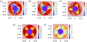
To give an impression of the large-scale flow patterns that develop at specific rotation rates, figure 2 shows (
 $\unicode[STIX]{x1D719},r$
) snapshots of temperature differences at different parameter points extracted from EULAG computations (
 $\unicode[STIX]{x1D719}$
as azimuth;
 $r$
as radius). Here, panel (a) (
 $Ta=5.79\times 10^{6}$
,
 $Ro=3.99$
) indicates a complex flow of coexisting wave modes
 $m=2$
and
 $m=3$
. Recent computations (von Larcher & Dörnbrack Reference von Larcher and Dörnbrack2015) and accompanying laboratory experiments (von Larcher & Egbers Reference von Larcher and Egbers2005) reported similar complex flows in the close neighbourhood of the parameter point, too. Previous studies have suggested that these complex flows may occur from nonlinear wave–wave interactions, including interference vacillations, sideband effects or resonant triad interaction, e.g. Ohlsen & Hart (Reference Ohlsen and Hart1989), Früh & Read (Reference Früh and Read1997).
The EULAG model. Maps in the (
 $\unicode[STIX]{x1D719},r$
) plane of the temperature difference, in K, at different parameter points (
 $Ta,Ro$
), showing large-scale wave modes of specific azimuthal wavenumber
 $m$
: (a)
 $Ta=5.79\times 10^{6}$
,
 $Ro=3.99$
, complex flow of
 $m=2$
and
 $m=3$
; (b)
 $Ta=12.25\times 10^{6}$
,
 $Ro=1.89$
,
 $m=3$
; (c)
 $Ta=16.68\times 10^{6}$
,
 $Ro=1.38$
,
 $m=3$
; (d)
 $Ta=28.13\times 10^{6}$
,
 $Ro=0.82$
,
 $m=4$
; (e)
 $Ta=129.59\times 10^{6}$
,
 $Ro=0.18$
,
 $m=4$
. It should be noted that the grid resolution is
 $192\times 192\times 67$
in
 $x$
,
 $y$
,
 $z$
, and the the colourbar has different scaling in each panel. Horizontal slices are taken just below the free top surface.

Beyond the abovementioned regimes, further remarkable flow characteristics such as, e.g., weak waves, dispersive waves, amplitude oscillations, shape or structural vacillations (SVs), have been observed by a number of laboratory and numerical studies. These complicated large-scale flow patterns are the result of generally nonlinear dynamic processes. Structural vacillations, in particular, occur near the transition to the fully irregular wave flow regime. Read et al. (Reference Read, Maubert, Randriamampianina and Früh2008) reported on temporal fluctuations of the flow that develops in the SV regime. These fluctuations are going to progressively disturb the regularity of the waves, which then leads to a transition to irregular waves with increasing rotation rate. A number of publications document the rich variety of the flow patterns that have been observed for the so-called Hide experiment, e.g. Pedlosky (Reference Pedlosky1970), Hide & Mason (Reference Hide and Mason1975), Hignett (Reference Hignett1985), Morita & Uryu (Reference Morita and Uryu1989), Read et al. (Reference Read, Bell, Johnson and Small1992), Früh & Read (Reference Früh and Read1997), Lu & Miller (Reference Lu and Miller1997), Pfeffer et al. (Reference Pfeffer, Applequist, Kung, Long and Buzyna1997), Früh (Reference Früh, von Larcher and Williams2015) and Read et al. (Reference Read, Perez, Moroz, Young, von Larcher and Williams2015).
Today, the annulus is still of interest for validating computational fluid dynamics codes incorporating new numerical concepts; see Vincze et al. (Reference Vincze, Borchert, Achatz, von Larcher, Baumann, Hertel, Remmler, Alexandrov, Egbers and Fröhlich2015). The Hide experiment is also an ideal testbed to study multiple-scale interactions. This might be due to the relatively simple geometry of the annulus, with well-defined boundary conditions, in contrast to the flows observed in the atmosphere, which are influenced by a large number of uncontrollable processes.
The study presented here is particularly concerned with the occurrence of small-scale features. These small-scale patterns are observed at both vertical sidewalls in regions where the jet stream interacts with the sidewall and is largely curved. We will particularly focus on the outer sidewall region, as the occurrence of small-scale phenomena in this region has not been discussed in previous studies to the best of the authors’ knowledge. However, we will also present results for the inner sidewall region when appropriate. The findings have been detected independently in direct numerical simulations with two different flow solvers, that is the geophysical flow solver EULAG and the higher-order compact (HOC) code. Furthermore, accompanying laboratory experiments show similar signals of small-scale instabilities. In order to preserve clarity, we only focus on a few particular parameter points even though our findings are observed for a broad range of parameters.
The paper is organized as follows. A survey of IGWs in a rotating baroclinic annulus is given in the next section. The numerical models and the laboratory set-up are described in § 3. The main results of the numerical simulations and the laboratory experiment are given in § 4. In § 5, possible mechanisms that may originate the small-scale instabilities are discussed. The paper then ends with a conclusion, § 6.
2 Inertia–gravity waves in a thermally driven rotating annulus
The existence of gravity waves in a thermally driven rotating annulus has recently been discussed by Jacoby et al. (Reference Jacoby, Read, Williams and Young2011), Borchert et al. (Reference Borchert, Achatz and Fruman2014) and Randriamampianina & Crespo del Arco (Reference Randriamampianina and Crespo del Arco2015). Jacoby et al. (Reference Jacoby, Read, Williams and Young2011) and also Randriamampianina & Crespo del Arco (Reference Randriamampianina and Crespo del Arco2015) reported that the observed small-scale instabilities, i.e. short-period waves, are located close to the inner sidewall of the annulus and are embedded in the large-scale baroclinic wave field. Jacoby et al. (Reference Jacoby, Read, Williams and Young2011) found that the short-period waves result from a localized instability of the thin thermal boundary layer and that they occur in regions of strong shear and downwelling tightly connected to the large-scale baroclinic wave flow. Randriamampianina (Reference Randriamampianina2013) and Randriamampianina & Crespo del Arco (Reference Randriamampianina and Crespo del Arco2015) proposed as generation mechanism a Kelvin–Helmholtz instability (KHI) invoking resonant over-reflection. That is, a density overturn was observed along the bottom boundary layer, associated with the presence of a reversal flow and a stagnation point, signalling the occurrence of KHI. There, IGWs result from the break of this KHI impinging on the inner cold wall.
Borchert et al. (Reference Borchert, Achatz and Fruman2014) investigated numerically emission of IGWs in two different configurations of the model set-up. The first set-up had a gap width
 $b-a=0.075~\text{m}$
and a fluid depth
 $d=0.135~\text{m}$
, with a lateral temperature difference of
 $\unicode[STIX]{x1D6E5}=8~\text{K}$
, denoted as the classic configuration. This set-up corresponds to an accompanied laboratory experiment (von Larcher & Egbers Reference von Larcher and Egbers2005; Harlander et al.
Reference Harlander, Larcher, Wang and Egbers2011). The second set-up, where
 $b-a=0.50~\text{m}$
,
 $d=0.04~\text{m}$
and
 $\unicode[STIX]{x1D6E5}=30~\text{K}$
, was used with the intent of studying the occurrence of IGWs in an atmosphere-like configuration, for which
 $N>f$
, where
 $N$
is the Brunt–Väisälä frequency and
 $f$
is the inertial frequency. In the real atmosphere,
 $N/f\approx 100$
, whereas
 $N/f<1$
in the classic configuration. In both configurations, the results indicated IGW activity close to the inner sidewall but also along the baroclinic wave front which seems to be emitted spontaneously.
Apart from Jacoby et al. (Reference Jacoby, Read, Williams and Young2011), who claimed to have found IGW activity by analysing time series data of a laboratory experiment, IGW activity in the classic experimental configuration of the rotating annulus has not been reported. This might be due the different scales in time and space of the equilibrated large-scale flow and the small-scale patterns. Furthermore, as IGWs apparently exist within the thin boundary layers as well, their weak signal might be a further objective for measurement techniques in laboratory experiments. However, signals of IGW activity have been reported by Read (Reference Read1992), and in mechanically forced two-layer fluid laboratory experiments on baroclinic waves, Lovegrove, Read & Richards (Reference Lovegrove, Read and Richards2000) and Williams et al. (Reference Williams, Haine and Read2008) have claimed to have detected IGWs. Formation of small-scale IGWs in the presence of baroclinic instability in a salt-stratified experiment was reported by Flór et al. (Reference Flór, Scolan and Gula2011). More recently, signatures of IGWs have been found in a thermohaline annulus experiment (Vincze et al. Reference Vincze, Borcia, Harlander and Le Gal2016).
It is interesting to note that short-period waves are also observed in similar rotating flow set-ups, e.g. in thermally driven Couette–Taylor systems. These set-ups are similar to the baroclinic annulus but with a much larger aspect ratio. Usually, the thermal Rossby number is too large to exhibit baroclinic instability, but interesting spiral structures have been observed (Leppiler et al. Reference Leppiler, Goharzadeh, Prigent and Mutabazi2008; Viazzo & Poncet Reference Viazzo and Poncet2014).
3 Numerical and experimental methods and parameters
The numerical simulations and laboratory experiments are performed by using the same model geometry. The gap width is 0.075 m, with
 $a=0.045~\text{m}$
and
 $b=0.120~\text{m}$
, and
 $d=0.135~\text{m}$
, where, as mentioned above,
 $a$
 $(b)$
is the inner (outer) radius and
 $d$
is the fluid depth. With these values, the radius ratio is calculated to be
 $\unicode[STIX]{x1D702}=0.375$
and the aspect ratio is
 $\unicode[STIX]{x1D6E4}=1.8$
. The Prandtl number is set to
 $Pr=7.0$
, i.e. we use the material properties of water for the fluid, in agreement with the laboratory set-up. All models consider a free top surface. However, the convective exchange between the fluid and the environment at the top surface is not taken into account in the numerical simulations. The equations are solved in a rotating reference frame, attached to the cavity, for the two codes.
3.1 The EULAG numerical model
The EULAG set-up used here has been previously used in the context of a parameter study of large-scale flow dynamics (von Larcher & Dörnbrack Reference von Larcher and Dörnbrack2015) and in the framework of a comprehensive benchmark test with respect to a laboratory reference experiment (Vincze et al. Reference Vincze, Borchert, Achatz, von Larcher, Baumann, Hertel, Remmler, Alexandrov, Egbers and Fröhlich2015). The governing partial differential equations are evaluated with a semi-implicit non-oscillatory forward-in-time differencing algorithm (Smolarkiewicz Reference Smolarkiewicz1991; Smolarkiewicz & Margolin Reference Smolarkiewicz and Margolin1997, Reference Smolarkiewicz and Margolin1998; Prusa, Smolarkiewicz & Wyszogrodzki Reference Prusa, Smolarkiewicz and Wyszogrodzki2008). The Navier–Stokes equations are solved in the Boussinesq approximation in the Eulerian flux-form advection scheme.
We use a Cartesian
 $(x,y,z)$
domain with physical lengths
 $0.258\times 0.258~\text{m}$
in the
 $x$
and
 $y$
directions and 0.135 m in the
 $z$
direction, where
 $z$
is the height. In this Cartesian domain, the annulus geometry is defined by using the usual conversion from Cartesian to polar coordinates. The grid dimension is set to
 $384\times 384\times 201$
in
 $x$
,
 $y$
,
 $z$
. This results in a grid resolution of
 $\unicode[STIX]{x0394}x=\unicode[STIX]{x0394}y=\unicode[STIX]{x0394}z=0.067\times 10^{-2}~\text{m}$
. The time step increment,
 $\unicode[STIX]{x0394}t$
, is set to
 $2.5\times 10^{-3}~\text{s}$
to ensure a small Courant–Friedrichs–Lewy (CFL) number.
The sidewalls and end walls of the annulus are modelled with the immersed boundary approach (Goldstein, Handler & Sirovich Reference Goldstein, Handler and Sirovich1993; Smolarkiewicz et al.
Reference Smolarkiewicz, Sharman, Weil, Perry, Heist and Bowker2007). At the sidewalls and at the bottom end wall as well, no-slip conditions are set, i.e.
 $\boldsymbol{U}=(u,v,w)=0$
, with
 $\boldsymbol{U}$
as the velocity vector, (
 $u,v$
) as its horizontal components and
 $w$
as its vertical component. At the free top end wall, only the vertical velocity component is bounded as
 $w=0$
; hence, we follow a free slip approach for the top boundary.
To model the lateral temperature difference,
 $\unicode[STIX]{x1D6E5}=T_{out}-T_{in}$
, with
 $T_{out}=+\unicode[STIX]{x1D6E5}/2$
and
 $T_{in}=-\unicode[STIX]{x1D6E5}/2$
relative to a reference temperature of
 $T=293.15~\text{K}$
, we set
 $T=T_{out}$
(
 $T_{in}$
), where the radius is equal to the outer (inner) radius of the research cavity. Rotation is implemented with the Coriolis parameter by default. The computations have been realized by, first, establishing the temperature difference in the research cavity while setting rotation rate to zero. Once the temperature difference has been established in the fluid, the rotation rate is set to the desired value.
3.2 The HOC code
The Navier–Stokes–Boussinesq equations are written in primitive variables for cylindrical coordinates. Conservation equations are solved on a fully staggered grid using a Fourier approximation in the homogeneous tangential direction. In the radial and vertical directions, the solutions are approximated using a fourth-order compact finite-difference scheme. The mesh in these two directions is refined near the boundaries using a hyperbolic tangent distribution (Abide & Viazzo Reference Abide and Viazzo2005).
The time advancement is second-order accurate and is based on the combination of an Adams–Bashforth for the convective terms with an implicit backward-Euler scheme for the viscous terms. The velocity–pressure coupling is solved using a projection algorithm. For each azimuthal wavenumber, the problem reduces at each time step to a set of 2D Helmholtz and Poisson equations (Oguic, Viazzo & Poncet Reference Oguic, Viazzo and Poncet2015). Equations are directly solved in their dimensional form.
For the imposed temperature gradient and the rotation rate considered here, a grid resolution composed of
 $131\times 181\times 384$
points in the radial, axial (vertical) and azimuthal directions has been used with a time step of
 $\unicode[STIX]{x0394}t=10^{-2}~\text{s}$
.
With this grid resolution, the thermal boundary layer, the thickness of which has been estimated a priori as 1.9 mm, cf. § 5.1, is described with 16 grid points in the radial direction, with a minimum mesh spacing of
 $\unicode[STIX]{x0394}r=0.1~\text{mm}$
. This high resolution guarantees that the wall layers are accurately resolved.
3.3 Laboratory experiment
The tank consists of three concentric cylinders mounted on a turntable (see figure 1). While the inner cylinder is made of anodized aluminium and is cooled by a thermostat, the middle and outer ones are made of borosilicate glass. The outer sidewall of the experiment gap is heated by a heating coil that is mounted at the bottom of the outer cylinder bath. The annulus has a flat bottom and free top surface. As working fluid, deionized water has been used. The experiment can be controlled via the rotation rate of the annulus,
 $\unicode[STIX]{x1D6FA}$
, and the temperature difference between the cooled inner and heated outer cylinders,
 $\unicode[STIX]{x1D6E5}=\overline{T}_{out}-\overline{T}_{in}$
.
A particle image velocimetry (PIV) system is used to measure the horizontal velocity components below the fluid surface; see Harlander et al. (Reference Harlander, von Larcher, Wright, Hoff, Alexandrov, Egbers, von Larcher and Williams2015). The surface temperature is measured by an infrared camera (InfraTec; spatial resolution
 $640\times 480$
pixels, thermal resolution
 ${<}0.08~\text{K}$
, spectral range
 $7.5{-}14~\unicode[STIX]{x03BC}\text{m}$
). The PIV system and infrared camera are mounted above the annulus on a corotating mast.
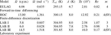
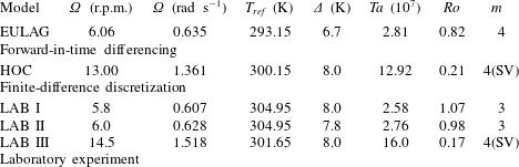
Parameters of the numerical simulations with the EULAG model and the HOC model, and of the laboratory experiments. Here,
 $\unicode[STIX]{x1D6FA}$
is the rotation rate,
 $T_{ref}$
is the reference temperature,
 $Ta$
is the Taylor number,
 $Ro$
is the thermal Rossby number and
 $m$
is the dominant azimuthal wavenumber of the large-scale flow; 4(SV) denotes a structural vacillation of a wavenumber 4 mode.
3.4 Parameters
For our study, we select different parameter points as given in table 1. These parameters are chosen with the purpose of studying small-scale instabilities in the wave flow regime, where we focus on a steady wave at moderate rotation rate and on an SV mode at higher rotation rate before the transition to geostrophic turbulence. The former is simulated by EULAG and the latter by HOC, and both regimes are studied in the laboratory experiment.
By inspecting the numerical simulations and the laboratory experiments we find some differences, particularly in the azimuthal wavenumber of the large-scale wave flow. This non-uniformity is not surprising but underlines the dynamics of the flow that under some circumstances could lead to baroclinic wave manifestations at similar parameter points, the so-called intransitivity phenomenon. For instance, an alteration of the zonal wavenumber is possible when the parameter point of interest is close to a transition between different wave modes with subsequent wavenumbers; see, e.g., von Larcher & Egbers (Reference von Larcher and Egbers2005).
The intransitivity phenomenon is not unique to the thermally driven rotating annulus but is inherent to confined rotating flows in general; see, e.g., Abrahamson, Eaton & Koga (Reference Abrahamson, Eaton and Koga1989). Regarding the thermally driven rotating annulus, multiple equilibria (different solutions for the same control parameter values
 $\unicode[STIX]{x1D6FA}$
and
 $\unicode[STIX]{x1D6E5}$
) have been found in several studies. Recently, in an extensive study, Vincze et al. (Reference Vincze, Borchert, Achatz, von Larcher, Baumann, Hertel, Remmler, Alexandrov, Egbers and Fröhlich2015) compared a number of numerical models with experimental data. From figure 6 in this paper it can be seen that there is a parameter region where an
 $m=3$
case coexists with the
 $m=4$
case. For
 $\unicode[STIX]{x1D6E5}=8~\text{K}$
, the region of coexistence starts at
 $\unicode[STIX]{x1D6FA}=6~\text{r.p.m.}$
and ends at approximately
 $\unicode[STIX]{x1D6FA}=16~\text{r.p.m.}$
; from then on, the system shows a unique
 $m=4$
solution. For the parameters chosen in the present study, multiple equilibria exist even for smaller
 $\unicode[STIX]{x1D6FA}$
. This is the reason why the experiment shows an
 $m=3$
and the simulation an
 $m=4$
case. However, the intention here is to demonstrate that the instabilities in the Stewartson layers are robust features occurring at different parameter points.
4 Results
We will begin this section with a phenomenological description of the small-scale flow patterns. Afterwards, we will consider quantitative measures. It is worth mentioning here that although we have chosen different values of
 $Ta$
and
 $Ro$
for the HOC and EULAG computations to cover different large-scale flows, the findings with respect to the small scales correspond very well, underlining that these wave-like features are generic and occur for quite different regimes of flow. In particular, very similar characteristics of the small-scale flow patterns have been found in the Stewartson layers, i.e. in regions close to the inner and outer vertical sidewalls of the annulus.
4.1 Small-scale features in the sidewall boundary layers
The notion ‘small-scale’ means here that we consider scales much smaller than the typical scale of the baroclinic wave, the latter of which is a fraction of the perimeter of the tank. The non-dimensional azimuthal wavenumber is between 3 and 4 in the cases we discuss. Nevertheless, we will see that the small-scale structures are tightly connected to the large-scale baroclinic wave.
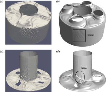
Isosurface snapshots of the small-scale instabilities in the vertical sidewall regions. (a,c) The EULAG model for
 $T=296.15~\text{K}$
(a) and
 $T=291.15~\text{K}$
(c). (b,d) The HOC model for
 $T=304.4~\text{K}$
(b) and
 $T=298.5~\text{K}$
(d). It should be noted that the holes in (b,c,d) are artificial in the sense they reflect that the specific value of the isosurface is not given there at the time increment shown.

Figure 3 shows temperature isosurfaces from a simulation with EULAG and HOC (see table 1). The isosurfaces have been chosen such that features close to the inner and outer sidewalls can be resolved and, moreover, the baroclinic wave is visible in the upper and lower parts of the annulus. It is obvious that at the cold inner wall, ripples can be found where the cold cyclones of the baroclinic wave touch the inner cylinder. At the warm outer sidewall, the ripples occur in the jet exit region which is just upstream of the cyclone. Both features are mainly restricted to the sidewall region. It should be noted that the structures are more pronounced in the EULAG model due to the different sidewall boundary conditions implemented in the models (see §§ 3.1 and 3.2).
The ripples at the outer heated wall have not been observed in previous studies and their origin and properties are unclear. In contrast to the ripples at the inner wall, which propagate downward while travelling with the baroclinic wave, the ripples at the outer wall form a nearly stationary wave packet which is slowly overtaken by the upstream front of the baroclinic wave. The ripples fade out close to the corresponding downstream part of the wave and form anew upstream; see figure 3. In this way, the wave packet is dragged along with the baroclinic wave. It is not obvious whether IGWs are emitted from the outer wall. We note that, while the velocity vectors are essentially tangential to the ripples at the inner wall, they are mainly perpendicular to the ripples at the outer wall, pointing to different mechanisms of instability. However, for the instability at the inner wall, it is known that IGWs can be emitted (Jacoby et al. Reference Jacoby, Read, Williams and Young2011; Randriamampianina Reference Randriamampianina2013; Randriamampianina & Crespo del Arco Reference Randriamampianina and Crespo del Arco2015) and that the local instability hence affects the bulk of the flow.
In order to detect more precisely the onset of the small-scale features observed towards the inner and outer sidewalls, we have carried out a series of computations using as initial conditions the time-averaged fields (associated with a low-pass filtering) obtained from solutions computed previously. This approach is aimed at identifying how these small-scale structures occur and propagate during the development of baroclinic motion. To detect these structures, we make use of the scalar
 $Q$
-criterion proposed by Hunt (Reference Hunt1987) and Hunt, Wray & Moin (Reference Hunt, Wray and Moin1988) to delineate coherent structures in turbulent flows. The
 $Q$
-criterion is defined by
 $$\begin{eqnarray}Q={\textstyle \frac{1}{2}}(||A||^{2}-||S||^{2}),\end{eqnarray}$$
where
 $||S||=[\text{tr}(SS^{t})]^{1/2}$
,
 $||A||=[\text{tr}(AA^{t})]^{1/2}$
, with
 $S$
and
 $A$
as the symmetric and antisymmetric parts of the velocity gradient tensor
 $\unicode[STIX]{x1D735}\unicode[STIX]{x1D650}$
respectively.
The HOC model. (a) Instantaneous isosurface of the
 $Q$
-criterion
 $Q=10^{-4}~\text{s}^{-2}$
with
 $Q\in [-1.9,1.0]~\text{s}^{-2}$
displayed in the unfolded cylinder with an orientation view in the
 $(\unicode[STIX]{x1D719},z)$
plane and a viewpoint from the inner sidewall,
 $\unicode[STIX]{x1D719}\in [0,2\unicode[STIX]{x03C0}]$
and
 $z\in [0,135]~\text{mm}$
(supplemental movie 1, available at https://doi.org/10.1017/jfm.2018.10). (b) Azimuth-time Hovmöller map of the
 $Q$
-criterion; data are taken at fluid depth
 $z=28~\text{mm}$
marked by the horizontal red line in (a). The vertical red line at
 $t=48~\text{s}$
indicates the time when the isosurface snapshot is taken.

The HOC model. (a) Instantaneous isosurface of the
 $Q$
-criterion
 $Q=10^{-4}~\text{s}^{-2}$
with
 $Q\in [-1.9,1.0]~\text{s}^{-2}$
displayed in the unfolded cylinder with an orientation view in the
 $(\unicode[STIX]{x1D719},z)$
plane and a viewpoint from the outer sidewall,
 $\unicode[STIX]{x1D719}\in [0,2\unicode[STIX]{x03C0}]$
and
 $z\in [0,135]~\text{mm}$
(supplemental movie 2). (b) As in figure 4, but the Hovmöller map is taken at fluid depth
 $z=52.4~\text{mm}$
, as marked by the horizontal red line in (a).

The HOC model. Snapshot of the tracks of particles 150 s after release. Four million particles are uniformly released in a (
 $\unicode[STIX]{x1D719},z$
) plane at radius
 $r=45.15~\text{mm}$
(supplemental movies 3 and 4). Particles are coloured by the local temperature: blue (red) colour
 $=$
cold (hot) temperature (K). The locations of IGWs at the inner sidewall (ripples at the outer one) are highlighted by ellipses (rectangles).

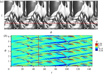
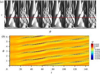
Figure 4, for the inner sidewall, and figure 5, for the outer one, show instantaneous isosurfaces of the
 $Q$
-criterion (a), and, in order to follow the evolutionary dynamics of the small-scale structures, corresponding time-azimuth maps (Hovmöller diagrams) are shown, too (b). The isosurfaces are displayed in the unfolded cylinder with an orientation view in the (
 $\unicode[STIX]{x1D719},z$
) plane including the radial direction to allow for the visualization of both small-scale and large-scale structures. The isosurface images, therefore, correspond to three-dimensional Cartesian representations in (
 $r,\unicode[STIX]{x1D719},z$
) at constant time, and the Hovmöller diagrams are time-azimuth maps at fixed radial and axial locations. The two isosurfaces correspond to the same specific value but, for the inner sidewall features, figure 4, the viewpoint of the isosurface is from the inner cylinder, while for the outer sidewall structures, figure 5, it is from the outer sidewall, therefore showing the large-scale waves towards the interior of the cavity. It should be noted that we have selected a specific range to magnify the small-scale structures in the Hovmöller plots and that in both figures the initial time step is the same.
Both figures underline the different characteristics of the small-scale features at the inner and outer sidewalls. For the inner sidewall, the isosurface diagram shows the small-scale structures between mid-depth and the bottom endwall which are inclined with respect to the horizontal. The corresponding Hovmöller plot (figure 4 b) shows that the structures evolve with a period of approximately 15 s, denoted by the horizontal plateaus. Afterwards, they start to propagate in a retrograde direction with respect to the large-scale baroclinic drift. At the outer sidewall, figure 5, the small-scale structures are organized in packets that are connected to the large-scale wave flow and propagate with it. Finally, these two phenomena exhibit the same temporal undulation which results from the oscillatory motion of the wave due to its SV characteristics. We have obtained a period of approximately 10 s for the small-scale features. Moreover, their shape appears to be more regular than the shape of the small-scale patterns at the inner sidewall.
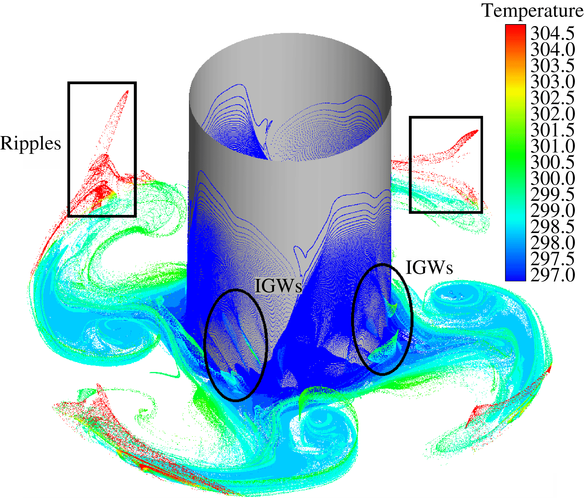
To get a better insight into the dynamics of the flow and to find possible links between the inner and outer small-scale features, Lagrangian tracers are implemented and their tracks are recorded. Four million particles are uniformly released in a (
 $\unicode[STIX]{x1D719},z$
) plane at radius
 $r=45.15~\text{mm}$
; thus, the position is located inside the inner sidewall boundary layer. Figure 6 displays a snapshot of the tracks, coloured by the local temperature, 150 s after their release. At the inner sidewall, the particles follow the downward flow (coloured dark blue due to the temperature of the inner sidewall), and they remain confined within the boundary layer until the occurrence of the small-scale structures. In this region, an overturn of the flow is detected as fluid of warmer temperature (coloured light blue–green), corresponding to these small-scale features, is located below areas with colder fluid (coloured dark blue). This phenomenon is also observed in figure 3, where the small-scale structures are indicated by the formation of ridges of constant temperature. Even if the small-scale structures propagate partly into the fluid interior, most of them are absorbed by the jet stream. At the outer sidewall, the small-scale features start to develop towards the bottom of the cavity when the outbound jet impinges at the outer sidewall. Following the red coloured paths corresponding to the temperature of the outer sidewall, they indicate that the small-scale features occur preferentially towards the anticyclonic cell and propagate upward while remaining confined along the outer sidewall. Regarding possible links between the inner and outer small-scale features, it is not evident yet whether the occurrence of one pattern triggers the formation of the other. However, this should be considered in more detail in future work.
By comparing figures 4, 5 and 6, we can conclude that at the cold inner sidewall, small-scale structures propagate downward not affected by the large-scale baroclinic wave. When arriving towards the bottom endwall, these features are attracted by the outbound jet with a strong acceleration, inducing a significant change in their local inclination with respect to the horizontal. The lack of particles along the inner wall, cf. figure 6, underlines the strong acceleration of the flow towards the formation of the jet. At the outer sidewall, the fluctuations are strongly attached to the large-scale wave. We found that these structures possess a different period in comparison with the inner features. Moreover, the outer sidewall structures show more regular spatial behaviour than those observed towards the inner sidewall, particularly in terms of inclination and wavelength.
The EULAG model. Horizontal structure of
 $\unicode[STIX]{x1D735}_{h}\boldsymbol{\cdot }\boldsymbol{v}$
in a mid-depth surface plot (a) and for a (
 $\unicode[STIX]{x1D719},z$
) cross-section extracted at
 $r=116~\text{mm}$
(4 mm from the outer sidewall) (b). It should be noted that white colour represents data in the interval [
 $-10^{-2},10^{-2}$
] that are masked out, and thus not printed, to highlight the small-scale features.

4.2 Gravity wave signature
When looking for the spatial signature of gravity waves in a large-scale flow, a natural choice is to plot the horizontal part of the divergence. Large-scale incompressible flows are nearly balanced, that is, close to the geostrophic equilibrium, characterized by a small Rossby number. (It should be noted that, here, we mean the usual Rossby number,
 $\unicode[STIX]{x1D716}=U/fL$
, and not the thermal Rossby number.) For such flows, the vertical velocity and in particular its vertical derivative,
 $\unicode[STIX]{x2202}w/\unicode[STIX]{x2202}z$
, is much smaller than the horizontal counterparts, and hence the horizontal divergence,
 $\unicode[STIX]{x1D735}_{h}\boldsymbol{\cdot }\boldsymbol{v}$
, is close to zero. Locally, however, the Rossby number can be of order one or larger, and then the vertical part of the divergence becomes important. This is the case for the velocity field of IGWs, which are typical structures for flows away from the geostrophic equilibrium.
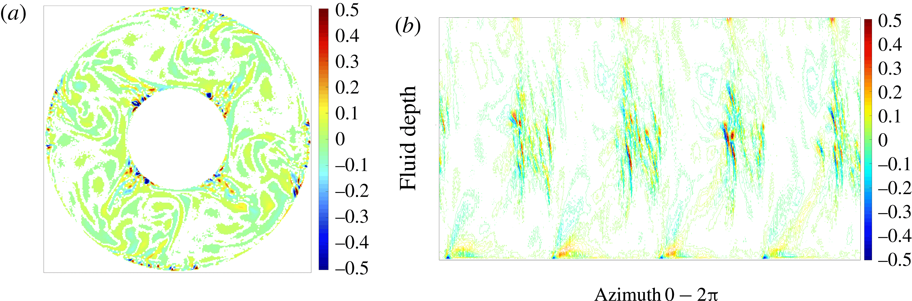
In figure 7, we plot the horizontal structure of
 $\unicode[STIX]{x1D735}_{h}\boldsymbol{\cdot }\boldsymbol{v}$
in a horizontal slice at mid-depth and in an axial–azimuthal plane close to the outer sidewall. From the horizontal section (figure 7
a), we clearly separate the small-scale features with a large
 $|\unicode[STIX]{x1D735}_{h}\boldsymbol{\cdot }\boldsymbol{v}|$
close to the boundaries, the vertical sidewalls, from the almost non-divergent flow in the bulk of the cavity. Clearly, the features are tightly connected to the baroclinic wave. However, the baroclinic wave front itself seems to be rather balanced and the instability is restricted to the boundary layers. In figure 7(b), we display the vertical structure of
 $\unicode[STIX]{x1D735}_{h}\boldsymbol{\cdot }\boldsymbol{v}$
. As mentioned before (by inspecting isosurfaces of the temperature field), we see that the rolls slope with respect to the axial direction, a typical feature for gravity wave packets. Obviously, the packet is strongest in mid-depth of the annulus.
Interestingly, in figure 7(b), we also see larger-scale structures in
 $\unicode[STIX]{x1D735}_{h}\boldsymbol{\cdot }\boldsymbol{v}$
at the top and bottom that have different characteristics from the ripples in mid-depth. They might be related to the enhanced vertical motion in regions where the horizontal flow interferes with the sidewall. However, it should be noted that the local ratio between the stratification parameter
 $N$
and the Coriolis parameter
 $f$
varies significantly along the outer wall. This can be seen in figure 3(c) in Borchert et al. (Reference Borchert, Achatz and Fruman2014). As described previously, these authors performed numerical simulations for an annulus with the same geometry as given in table 1 and with
 $\unicode[STIX]{x1D6E5}=8~\text{K}$
and
 $\unicode[STIX]{x1D6FA}=6~\text{r.p.m}$
. The value of
 $N/f$
shows a local maximum of approximately
 $0.5$
at the corner formed by the bottom and the outer sidewall. In the corresponding upper corner, the ratio reduces to
 $N/f\approx 0.1$
. This change in stability has a strong impact on the characteristics of IGWs: two waves with the same frequency have, e.g., an angle of
 $45^{\circ }$
at the bottom but nearly
 $90^{\circ }$
at the top, where the angle is measured between the orientation of the wave crest and the horizontal. Hence, in our study, the structures at the bottom and the top might also be signatures of gravity waves generated by the same or a different kind of instability from the ripples at mid-depth.
In summary, we can say that the instability that takes place at the outer sidewall is manifested in the form of ripples and rolls reminiscent of gravity wave packets, trapped in the axial direction and showing a significant amplitude mainly in mid-depth of the Stewartson boundary layer.
4.3 Multiscale flow structure in the outer wall layer
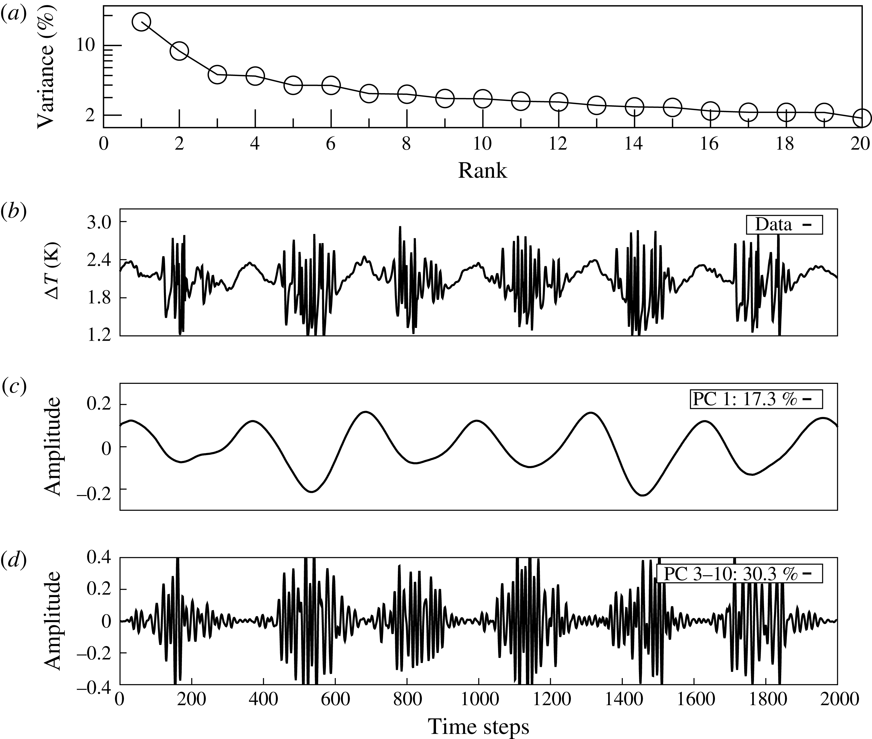
In § 4.1, we have shown that the onset of the small-scale features is linked with the onset of the large-scale baroclinic wave. To analyse the small-scale patterns in a settled wave mode, we make use of the singular spectrum analysis (SSA) technique and use the toolkit by Vautard, Yiou & Ghil (Reference Vautard, Yiou and Ghil1992), Dettinger et al. (Reference Dettinger, Ghil, Strong, Weibel and Yiou1995) and Ghil et al. (Reference Ghil, Allen, Dettinger, Ide, Kondrashov, Mann, Robertson, Saunders, Tian and Varadi2002). Here, an oscillatory mode is characterized by a pair of nearly equal eigenvalues (EVs).
We use the EULAG data and take a time series of temperature difference at radius
 $r=118.6~\text{mm}$
(1.4 mm from the outer sidewall) and at fluid depth
 $d=54~\text{mm}$
. The sampling time is approximately 950 s. We set the window length
 $M$
, that is the number of temporal lags, to
 $M=100$
(approximately 5 % of the data). It should be noted that we also performed some tests with smaller and larger temporal lags to prove the robustness of the results.
The results of the SSA are given in figure 8. Figure 8(a) shows the eigenvalue spectrum of the SSA covariance matrix. The first EV explains approximately 17 % of the total variance of the data series, representing in part the large-scale
 $m=4$
wave flow; cf. figure 8(c). It should be noted that the second EV, approximately 8 % of the total variance, also represents a part of the large-scale flow. The small-scale structures are represented by EVs 3–10, arranged in four pairs, with a cumulative variance of approximately 30 %. For larger EVs, we find the noisy tail of the EV spectrum. Figures 8(c) and 8(d) show the appropriate reconstruction of the time series for EV 1 and the cumulative one for EVs 3–10. The small-scale patterns appear as short-period wave trains.
Strikingly, the amplitude of the envelope of these wave trains grows in conjunction with the cooling cycle of the large-scale mode in figure 8(c), and it decreases during the heating cycle. This feature does not only underline the previous findings, that, at the outer sidewall, the small-scale patterns occur mainly prefrontal to the jet stream and not within the anticyclonic warm cycle; the time series analysis, furthermore, documents that the large-scale baroclinic wave flow and the small-scale patterns act as a nearly steady state and multiscale flow system.
The EULAG model. The SSA of temperature time series data taken at
 $d=54~\text{mm}$
and
 $r=118,6~\text{mm}$
. (a) The EV spectrum (variance over rank); (b) data time series; (c) reconstruction with EV 1; (d) as (c) but with EVs 3–10. The proportion of variance is as given in (c) and (d). One should note the different amplitude ranges in (c) and (d).

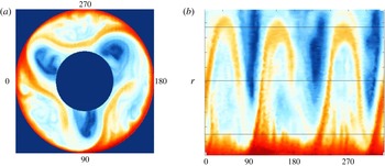
Laboratory experiment, LAB I. The surface temperature field experimentally observed by using an infrared camera. Camera view (a) and view in polar coordinates (b) with the azimuth at the abscissa and the radius at the ordinate. The outer sidewall is at the bottom and the inner sidewall is at the top. The labels at the abscissa reflect the azimuth positions given in (a).

4.4 Experimental results
In the following, we briefly describe results from the laboratory experiments given in table 1. Figure 9 shows the surface temperature of LAB I measured by an infrared camera that was mounted above the rotating annulus (camera view (a); view in polar coordinates (b)). The annulus rotates in the anticlockwise direction. The large-scale structure is dominated by three cold cyclones forming a baroclinic wave of dominant azimuthal wavenumber
 $m=3$
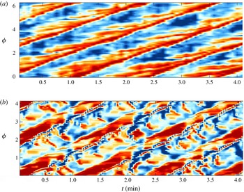
. This pattern is propagating anticlockwise too but slightly faster than the annulus rotation, called prograde propagation. One should note the similarity with the numerical simulation in figure 2(b,c). Clearly visible is also the warm jet that circles around the baroclinic wave. The jet velocity is strongest in the jet exit region, which is just upstream of the cyclone close to the outer heated wall. Just ahead of this region, at the outer boundary, we observe small-scale wave-like features. The structure is reminiscent of Görtler-type instability, and its position corresponds well with the small-scale divergence signal visible in figure 7(top), although, due to the no-heat-flux upper boundary conditions in the numerical simulation, the signal is rather weak close to the surface. This has already been discussed in a comprehensive benchmark study by Vincze et al. (Reference Vincze, Borchert, Achatz, von Larcher, Baumann, Hertel, Remmler, Alexandrov, Egbers and Fröhlich2015). It should be noted that outside the jet, between the cold cyclones, weak anticyclones form. This implies that in front of the jet exit region, a strong shear can be found.
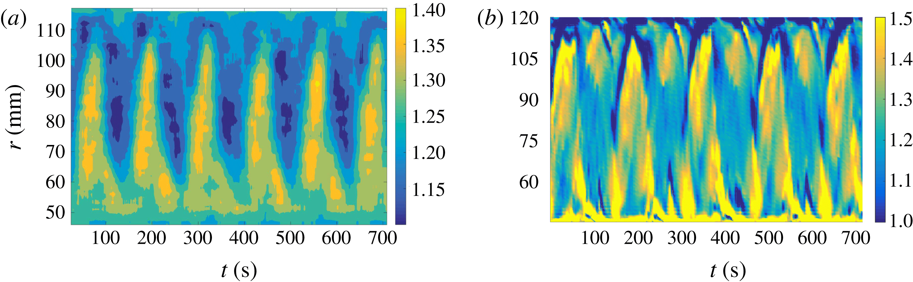
To see the phase velocity of the small-scale features, we display a time–space (Hovmöller) diagram of the temperature anomaly in figure 10(a). The temperature data have been taken from a ring approximately one centimetre away from the outer heated sidewall and plotted over a period of 5 min. The baroclinic wave is clearly visible, but also the small-scale features upstream of the wave. Obviously, they propagate slower than the baroclinic wave. The ripples can also be interpreted as an almost stationary wave packet that is overtaken by the jet at one end and arises anew at the other end. Directly above the warm baroclinic wave crest, there is an even smaller-scale pattern that moves with the baroclinic wave. All of the structures described above can also be seen in the corresponding EULAG simulation although with differences in their manifestation (see figure 10 b): (i) the intermittent warm crests of the baroclinic waves, (ii) the small-scale structures in front of the baroclinic wave, and (iii) the smaller-scale pattern that moves with the baroclinic wave. The differences are that (i) the baroclinic wave has wavenumber 4 and not 3 (see also table 1) due to the existence of multiple equilibria for the chosen parameters; (ii) in contrast to the experiment, most of the small-scale structures in front of the baroclinic wave crests propagate in a retrograde direction. It should be noted that part of this difference is due to the different flow regimes we find for basically the same parameters (multiple equilibrium). However, it is important to note that the top free surface boundary condition imposed in the numerical model differs from that in the laboratory experiment. In the numerical model, a zero-temperature flux condition together with free slip is applied. In the experiment, a non-zero surface heat flux occurs due to the open surface. Discrepancies in the temperature are for some part inferred from these differences. Nevertheless, in spite of the differences, we wanted to compare the experimental and numerical results to highlight that the major features can be found for both cases. It should be noted further that the wave packets shown for the divergence field in figure 7(b) are nearly stationary in the rotating frame of reference and the features at the surface might not be directly linked to them.
Azimuth-time (Hovmöller) maps. Comparison of the small-scale structures in the laboratory experiment and in the EULAG simulations. (a) Laboratory experiment, LAB II, surface temperature anomaly 10 mm away from the outer sidewall measured by the infrared camera; the mean temperature of
 $304.95~\text{K}$
has been subtracted. (b) The EULAG temperature difference 4 mm away from the outer sidewall 7 mm below the surface. Here, the mean temperature difference has been subtracted and afterwards data are gained. It should be noted that the large-scale flow is
 $m=3$
in the experiment and
 $m=4$
in EULAG. Therefore, the azimuth is cropped in (b) for comparison with the experiment.

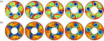
Figure 11 shows (
 $\unicode[STIX]{x1D719},r$
) maps of the instantaneous temperature field for laboratory measurements (LAB III) (a) obtained at
 $\unicode[STIX]{x1D6FA}=14.5~\text{r.p.m.}$
and for the HOC computations (b) at
 $\unicode[STIX]{x1D6FA}=13~\text{r.p.m.}$
Both parameter points are in the SV regime. The images are taken at different times covering approximately one-quarter of the baroclinic drift period, and the HOC images are taken 10 mm below the free top surface. It is important to note that also in the HOC computations the top free surface boundary condition imposed differs from that in the laboratory experiment, where a non-zero surface heat flux occurs. Discrepancies in the temperature are for some part inferred from these differences. However, both the experiment and the numerics show very similar dynamics, and both approaches exhibit the same strong swirl developing inside the cyclonic cold cells. We further observe that the oscillatory flapping of the cold vortices, a typical feature of SV wave modes, is not symmetric.
Comparison of HOC simulations and results from the laboratory experiment. (a) Thermographic images of the surface temperature in the LAB III experiment. (b) Isocontours of the temperature field in the HOC simulations.

4.5 Summary of our findings
To summarize our findings regarding the small-scale instabilities, the data analysis reveals interesting features of the small-scale patterns. That is, (1) they give a small but significant signal in the direct measures such as, e.g., temperature difference, and they are also evident in indirect measures such as, e.g., horizontal divergence; (2) at the (inner) outer sidewall, they occur where the jet stream turns (outbound) inbound, i.e. where the jet is curved towards the fluid interior; (3) they are inclined with respect to the horizontal; (4) they are mainly restricted to the wall layer region; (5) they occur throughout the entire fluid depth, with the strongest signal at the outer sidewall between
 $z=0.3\,d$
and
 $z=0.8\,d$
; (6) they are connected with the large-scale baroclinic flow. It should be noted that in the inner sidewall region, the small-scale patterns mainly occur between the bottom and mid-depth rather than above mid-depth. In the next section, we try to form a coherent quantitative picture of instabilities that are responsible for the small-scale wavy structures.
5 Discussion
In the previous section, we presented qualitative findings of small-scale instabilities at the inner and outer sidewalls of the thermally driven rotating annulus and described their characteristics. At first glance, the listed features are similar to the findings in the abovementioned publications by Jacoby et al. (Reference Jacoby, Read, Williams and Young2011), Borchert et al. (Reference Borchert, Achatz and Fruman2014) and Randriamampianina & Crespo del Arco (Reference Randriamampianina and Crespo del Arco2015), although the authors were not aware of the small-scale instabilities at the outer sidewall but had discussed inner sidewall instabilities. In this section, we discuss some mechanisms that are candidates for generating the small-scale wave-like structures at both the inner and the outer sidewall boundary layers. In particular, we focus on thermal instability and on inertial or rotational instability. We will also discuss the nature of the small-scale features as being IGWs.
5.1 Thermal boundary layer instability
Let us first check whether our results are consistent with the results presented by Jacoby et al. (Reference Jacoby, Read, Williams and Young2011) for the inner sidewall instabilities. Barcilon & Pedlosky (Reference Barcilon and Pedlosky1967) found two specific parameters that play an important role in the relative contributions of the different boundary layers to the heat transfer from the sidewall into the fluid interior. The first parameter is the Ekman number, here defined as
 $Ek=\unicode[STIX]{x1D708}/\unicode[STIX]{x1D6FA}d^{2}$
; the second parameter is the product of the thermal Rossby number and the Prandtl number,
 $(Ro\,Pr)$
. For the EULAG set-up, it follows that
 $$\begin{eqnarray}Ek=8.74\times 10^{-5},\quad (Ro\,Pr)=0.82\times 7.0=5.74;\end{eqnarray}$$
thus,
 $Ek\ll (RoPr)$
.
Now, we consider the extent of boundary layers at the vertical sidewalls, that is, the viscous Stewartson layer,
 $\unicode[STIX]{x1D6FF}_{\unicode[STIX]{x1D708}}$
, and the thermal boundary layer,
 $\unicode[STIX]{x1D6FF}_{T}$
. Following James, Jonas & Farnell (Reference James, Jonas and Farnell1980), we calculate
 $\unicode[STIX]{x1D6FF}_{\unicode[STIX]{x1D708}}=(b-a)~\sqrt[3]{Ek}=3.3~\text{mm}$
.
In von Böckh & Wetzel (Reference von Böckh and Wetzel2014), an empirical formula for the calculation of the thermal boundary layer thickness along a heated vertical wall for a laminar flow is given. This formula reads as
 $$\begin{eqnarray}\unicode[STIX]{x1D6FF}_{T}=\frac{L}{Nu},\end{eqnarray}$$
where
 $L$
is the length of the wall. Here,
 $Nu$
is the Nusselt number,
 $$\begin{eqnarray}Nu=(0.852+0.387Ra^{1/6}F)^{2},\end{eqnarray}$$
with
 $Ra$
as the Rayleigh number,
 $Ra=(Pr\,Ta\,Ro)/4$
. The parameter
 $F$
is related to the Prandtl number and reads as
 $$\begin{eqnarray}F=(1+0.671Pr^{(-9/16)})^{(-8/27)}.\end{eqnarray}$$
In the literature, this approach has been used for a large range of
 $Pr$
and
 $Ra$
. Following this ansatz, we calculate the thickness of the thermal boundary layer as
 $\unicode[STIX]{x1D6FF}_{T}=1.9~\text{mm}$
, which is in good agreement with the well-known formula for the convective heat transport in a laminar flow,
 $Pr^{1/3}=\unicode[STIX]{x1D6FF}_{\unicode[STIX]{x1D708}}/\unicode[STIX]{x1D6FF}_{T}$
, with
 $\unicode[STIX]{x1D6FF}_{\unicode[STIX]{x1D708}}$
as calculated above. Obviously, the viscous boundary layer is significantly thicker than the thermal boundary layer. These values of the boundary layer thicknesses have been used to provide a first estimate of the adequate numerical grid resolution necessary to compute a well-resolved solution in sidewall boundary regions.
Generally, the extent of the equilibrated large-scale baroclinic waves is constrained by the Stewartson layers, and if the Stewartson layers are thicker than the thermal boundary layers, the feedback between the sidewall temperature forcing and the baroclinic waves is weak and most of the imposed temperature gradient is handled in the thermal boundary layer; see Früh (Reference Früh, von Larcher and Williams2015).
McBain, Armfield & Desrayaud (Reference McBain, Armfield and Desrayaud2007) analysed the instability of the buoyancy layer on an evenly heated vertical wall for a stratified fluid with different Prandtl numbers. They found that above a critical value of a local Reynolds number,
 $Re_{c}$
, the flow becomes unstable and supports two-dimensional travelling waves. For a fluid of
 $Pr=7$
, they determined
 $Re_{c}\approx 8.58$
. Following the ansatz by Jacoby et al. (Reference Jacoby, Read, Williams and Young2011), we estimate a local Reynolds number with
 $$\begin{eqnarray}Re_{local}=\frac{|w|~\unicode[STIX]{x1D6FF}_{T}~\sqrt{2}}{\unicode[STIX]{x1D708}}=2.676~|w|,\end{eqnarray}$$
where
 $w$
is the vertical component of the velocity. Thus, local maxima of the Reynolds number are linked with large values of vertical velocity.
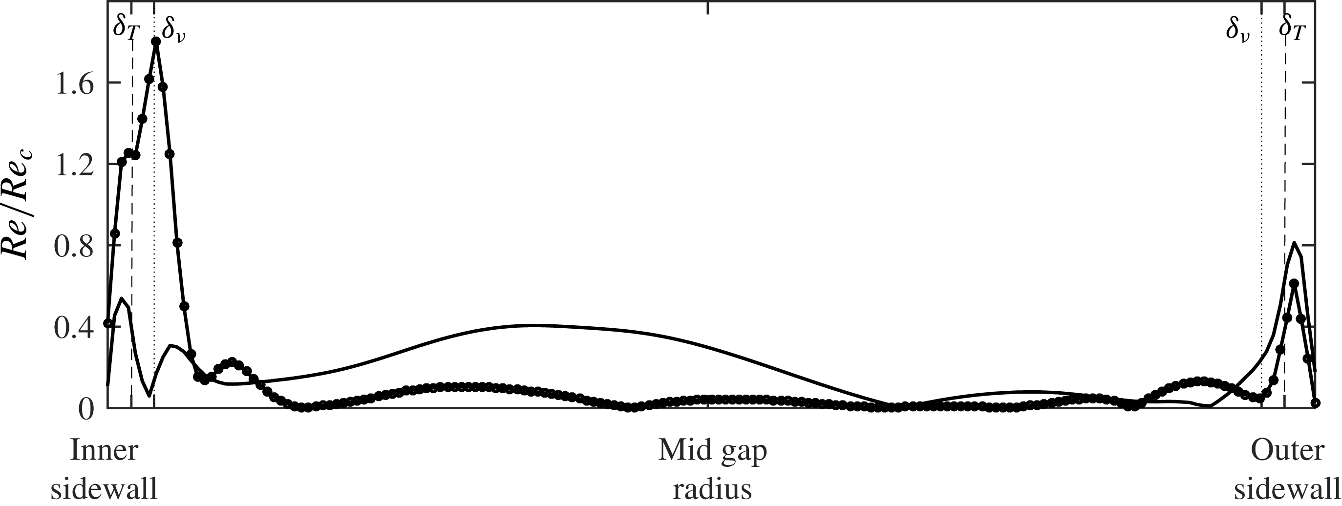
Figure 12 shows an exemplary line plot of
 $Re_{local}/Re_{c}$
along two cross-sections, through an inner and an outer sidewall instability, extracted at
 $z=0.36\,d$
, i.e.
 ${\approx}50~\text{mm}$
above the bottom end wall. In the inner sidewall boundary layers, Stewartson and thermal boundary layers, the instability condition is fulfilled for the inner sidewall instability profile (since
 $Re_{local}/Re_{c}>1$
) but not for the outer one. At the outer sidewall, the instability condition is not fulfilled, either in the profile through the outer or through the inner sidewall instability. (It is worth mentioning that the peaks of the graphs align well with the calculated thickness of
 $\unicode[STIX]{x1D6FF}_{T}$
and
 $\unicode[STIX]{x1D6FF}_{\unicode[STIX]{x1D708}}$
.)
Even if the study of McBain et al. (Reference McBain, Armfield and Desrayaud2007) is concerned with non-rotating flows, we see that the boundary layer instability theory supports the development of small-scale instabilities at the inner sidewall but not at the outer sidewall.
The EULAG model. Radial cross-sections of the local Reynolds number scaled with
 $Re_{c}$
. The profiles are taken at
 $z=0.36\,d$
and at specific azimuthal positions with a cut through an inner sidewall instability (–
 $\bullet$
–) and through an outer one (——). At both sidewalls, the calculated thicknesses of the thermal and viscous boundary layers are indicated by vertical lines: thermal boundary layer
 $\unicode[STIX]{x1D6FF}_{T}$
(dashed lines); viscous boundary layer
 $\unicode[STIX]{x1D6FF}_{\unicode[STIX]{x1D708}}$
(dotted lines).

5.2 Inertial instability
At both sidewalls, the small-scale instabilities arise where the large-scale jet flow is turned towards the fluid interior. Hence, there, close to the sidewalls, the horizontal flow is strongly sheared and, additionally, in part retrograde. Under such conditions, the flow might result in inertial or rotational instability.
A necessary condition for instability in an ideal fluid, basically inviscid, was discovered by Rayleigh (Reference Rayleigh1917). It is based on the equilibrium between the centrifugal force and the radial pressure gradient. The Rayleigh criterion states that a flow is unstable when the velocity profile,
 $U(r)$
, has an inflection point, i.e. where
 $\unicode[STIX]{x2202}^{2}U/\unicode[STIX]{x2202}r^{2}~=0$
. It should be noted that Synge (Reference Synge1933) and Tollmien (Reference Tollmien1935) have strengthened the criterion to a sufficient condition. Originally developed for plane-parallel axisymmetric flows, the Rayleigh criterion was recently generalized for non-axisymmetric flows; see, e.g., Billant & Gallaire (Reference Billant and Gallaire2005).
For more general rotating flows, however, it is known that the Rayleigh criterion is not strictly correct. For example, the Rayleigh criterion does not incorporate instability of a flow showing density variations or axial shear. To investigate boundary layer instability in a rotating cylindrical tank, Hart & Kittelman (Reference Hart and Kittelman1996) considered an experiment where the upper lid rotates somewhat faster than the tank. For this mechanically driven flow, the Stewartson layer shows azimuthal and axial shear. In a thermally driven rotating annulus, an axial shear in the bulk of the fluid is given due to the baroclinic state of the system. Moreover, application of the Hart criterion to the sidewall instabilities implies the assumption that the radial shear in the jet region at the sidewalls is much higher than the axial shear, which, in consequence, is neglected. However, it is observed that the axial velocity component,
 $U_{z}$
, becomes significant towards the inner and outer sidewalls, i.e. where the small-scale instabilities appear. Hart & Kittelman (Reference Hart and Kittelman1996) proposed a criterion that takes into account the effect of the axial velocity component in the rotating reference frame, involving the Coriolis shear instability mechanism. This condition reads as
 $$\begin{eqnarray}\unicode[STIX]{x1D6F7}^{\prime }(r)=2\unicode[STIX]{x1D6FA}\cos (\unicode[STIX]{x1D6FE})\left(2\unicode[STIX]{x1D6FA}\cos (\unicode[STIX]{x1D6FE})+\frac{\text{d}U^{\prime }}{\text{d}r}\right)<0,\end{eqnarray}$$
where
 $\tan (\unicode[STIX]{x1D6FE})=U_{z}/U_{\unicode[STIX]{x1D719}}$
and
 $U^{\prime }$
is the velocity magnitude tangent to the wall at angle
 $\unicode[STIX]{x1D6FE}$
, with
 $U^{\prime }=\sqrt{U_{\unicode[STIX]{x1D719}}^{2}+U_{z}^{2}}$
.
Radius–time Hovmöller plot of
 $\unicode[STIX]{x1D6F7}^{\prime }(r)$
, (5.6), but with
 $U_{z}=0$
. (a) Experimental LAB II PIV data at fluid depth
 $d=80~\text{mm}$
(55 mm below the free top surface); (b) EULAG model data at fluid depth
 $d=98~\text{mm}$
(37 mm below the top surface). It should be noted that the inner sidewall is at
 $r=45~\text{mm}$
and the outer one at
 $r=120~\text{mm}$
.

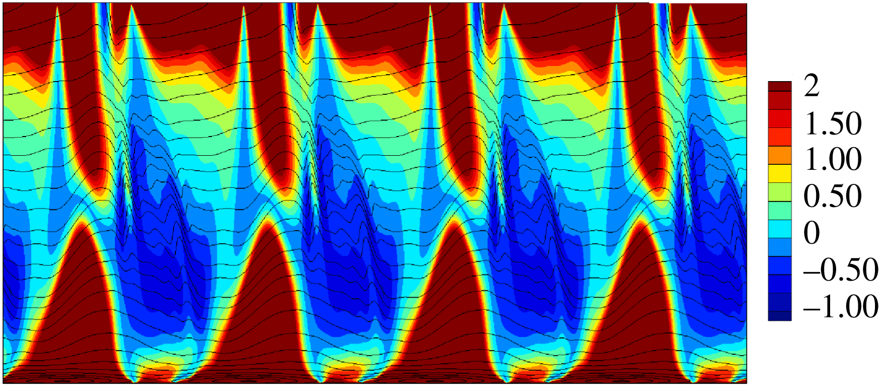
The HOC model. A
 $(\unicode[STIX]{x1D719},z)$
-plot of
 $\unicode[STIX]{x1D6F7}^{\prime }(r)$
, (5.6), at radius
 $r=119.3~\text{mm}$
. Here,
 $\unicode[STIX]{x1D6F7}^{\prime }(r)$
is represented by colours and lines correspond to isotherms.

Figure 13 shows radius–time Hovmöller diagrams of the left-hand side of (5.6) for the LAB II case and for EULAG data when we assume
 $U_{z}=0$
. Obviously, for this simplified situation, the boundary layer is stable since (5.6) is not fulfilled as the left-hand side is positive everywhere. It should be noted that we observe the same in subsurface sections below mid-depth (not shown). However, this changes dramatically when we include the shear of the axial flow. Figure 14 shows the variation of the adapted generalized Rayleigh discriminant
 $\unicode[STIX]{x1D6F7}^{\prime }(r)$
, the left-hand side of (5.6), in a
 $(\unicode[STIX]{x1D719},z)$
diagram. The HOC data have been taken at radius
 $r=119.3~\text{mm}$
, which is close to the outer wall where the intensity of the small-scale structures is highest. The Coriolis shear instability condition is fulfilled, that is,
 $\unicode[STIX]{x1D6F7}^{\prime }(r)$
is negative in the region where the ripples are dominant and particularly in the mid-depth area, as revealed by the variations of the isocontours of temperature. This result is in good agreement with the signature of the horizontal divergence shown in figure 7.
It is worth recalling that centrifugal instability and Coriolis shear instability correspond here to the same phenomenon, as both refer to the same criterion, e.g. Chomaz et al. (Reference Chomaz, Ortiz, Gallaire, Billant and Flór2010), although the Coriolis shear mechanism is more generally invoked in a rotating reference frame.
From the analysis of both circulation criteria, we conclude that the small-scale instabilities at the outer sidewall, but not at the inner sidewall, are generated by an inertial instability rather than by an instability of the thermal boundary layer.
5.3 Inertia–gravity waves
In the previous sections, we have shown that the small-scale patterns at the inner and outer sidewalls are probably generated by different instability mechanisms. Finally, in this section, we discuss the possibility that the small-scale structures are a gravity wave signal. As described above, it has previously been claimed that IGWs have been found at the inner sidewall in the classic rotating annulus set-up. It is, therefore, reasonable to examine whether the small-scale patterns at the outer sidewall are IGWs, too. The discussion is based on the IGW dispersion relation, which reads as (cf. Gill Reference Gill1982; Fritts & Alexander Reference Fritts and Alexander2003)
 $$\begin{eqnarray}\widetilde{\unicode[STIX]{x1D714}}=(\unicode[STIX]{x1D714}-\boldsymbol{U}\boldsymbol{\cdot }\boldsymbol{k})=\pm \sqrt{\frac{N^{2}(k^{2}+l^{2})+f^{2}m^{2}}{k^{2}+l^{2}+m^{2}}},\end{eqnarray}$$
with
 $N=\sqrt{g\unicode[STIX]{x1D6FC}\unicode[STIX]{x1D6FF}T/\unicode[STIX]{x1D6FF}z}$
as the Brunt–Väisälä buoyancy frequency (
 $\unicode[STIX]{x1D6FF}T/\unicode[STIX]{x1D6FF}z$
as the vertical temperature gradient) and
 $f=2\unicode[STIX]{x1D6FA}$
as the Coriolis parameter. The intrinsic frequency,
 $\widetilde{\unicode[STIX]{x1D714}}$
, corresponds to the one that would be observed in a frame moving with the background flow, here the large-scale baroclinic wave flow. The
 $+$
prefix denotes positive and the
 $-$
prefix negative (retrograde) phase speeds. For positive
 $\widetilde{\unicode[STIX]{x1D714}}$
, the IGW frequency range reads as
 $N<\widetilde{\unicode[STIX]{x1D714}}<f$
, and for negative
 $\widetilde{\unicode[STIX]{x1D714}}$
, the IGW criterion reads as
 $-N>\widetilde{\unicode[STIX]{x1D714}}>-f$
.
The Doppler frequency
 $\boldsymbol{U}\boldsymbol{\cdot }\boldsymbol{k}$
is
 $$\begin{eqnarray}\boldsymbol{U}\boldsymbol{\cdot }\boldsymbol{k}=(U_{\unicode[STIX]{x1D719}},U_{r},U_{z})\cdot (k,l,m)=U_{\unicode[STIX]{x1D719}}k+U_{r}l+U_{z}m,\end{eqnarray}$$
with
 $U_{\unicode[STIX]{x1D719}}$
as the azimuthal,
 $U_{r}$
as the radial and
 $U_{z}$
as the axial velocity component, and
 $k,l,m$
as the azimuthal, radial and axial wavenumbers. The Doppler frequency occurs in the frame of reference moving with the rotating annulus, where
 $\unicode[STIX]{x1D714}$
is the measured frequency of the small-scale ripples.
In the following analysis, the wavenumbers are estimated from cross-sections of instantaneous fluctuation fields. The inner sidewall features also are located very close to the inner wall but have a 3D structure as they propagate into the fluid interior. We focus on the HOC computations for the IGW analysis at the inner sidewall and use the EULAG data for the analysis at the outer sidewall. With this, we consider both the flow regime at moderate rotation rate (EULAG) and the SV flow regime at higher rotation rate (HOC).
From the HOC computations, we obtain a drift frequency of
 $\unicode[STIX]{x1D714}_{d}\approx 0.02~\text{rad}~\text{s}^{-1}$
for the large-scale baroclinic wave mode, and from figure 4 we observe a retrograde phase speed of frequency
 $\unicode[STIX]{x1D714}_{g}\approx -0.42~\text{rad}~\text{s}^{-1}$
for the small-scale instabilities (obtained in the frame rotating with the cavity). To determine the nature of the small-scale features,
 $\unicode[STIX]{x1D714}_{g}$
can be compared with another value provided independently from the Doppler effect involving the intrinsic gravity wave frequency,
 $\widetilde{\unicode[STIX]{x1D714}}$
; see (5.7).
The dimensional values of the wavenumbers are estimated to be
 $k=6.27~\text{cm}^{-1}$
,
 $l=10.47~\text{cm}^{-1}$
and
 $m=3.25~\text{cm}^{-1}$
. The value of the zonal wavenumber
 $k$
is taken at a radius of
 $r_{bl}=0.005~\text{m}$
, i.e. 5 mm from the inner sidewall, corresponding to the location of the highest intensity of the inner sidewall small-scale fluctuations. Here, an estimate of the buoyancy frequency yields
 $N\approx 0.78~\text{rad}~\text{s}^{-1}$
, which results in an
 $N/f$
ratio of
 $N/f\approx 0.29$
, with
 $f=2.72~\text{rad}~\text{s}^{-1}$
. With this, the intrinsic frequency is calculated to be
 $\widetilde{\unicode[STIX]{x1D714}}\approx -1.03~\text{rad}~\text{s}^{-1}$
.
For the small-scale instabilities using the Doppler relation,
 $\unicode[STIX]{x1D714}=\widetilde{\unicode[STIX]{x1D714}}+k\,U$
, since at the inner sidewall the motion of the background flow corresponds to the uniform drift of the baroclinic waves in the zonal direction
 $U_{\unicode[STIX]{x1D719}}=r_{bl}\unicode[STIX]{x1D714}_{d}$
. With this, we determine a gravity wave frequency of
 $\unicode[STIX]{x1D714}\approx -0.52~\text{rad}~\text{s}^{-1}$
, which is in good agreement with
 $\unicode[STIX]{x1D714}_{g}$
. Exact agreement cannot be expected due to the wave variability, and, furthermore, keeping in mind that wavenumbers are estimated from instantaneous fields.
Now, we inspect the ripples at the outer wall and examine whether they are locally consistent with the IGW dispersion relation, too. From the EULAG numerical simulation, we know that the ripples are attached to the baroclinic wave and hence move roughly with the same speed, that is,
 $c\approx 0.004~\text{m}~\text{s}^{-1}$
. The azimuthal wavenumber of the large-scale flow is estimated to be
 $k_{d}\approx 5~\text{m}^{-1}$
; this gives an angular frequency of
 $\unicode[STIX]{x1D714}_{d}=c\,k_{d}=0.02~\text{rad}~\text{s}^{-1}$
. The wavelength of the ripples,
 $\unicode[STIX]{x1D706}$
, aligned at roughly
 $45^{\circ }$
with respect to the horizontal direction, is approximately
 $0.005~\text{m}$
, implying
 $k=m\approx 10^{3}~\text{m}^{-1}$
, where
 $l=0$
, as mentioned above. This gives a frequency of
 $\unicode[STIX]{x1D714}_{g}=c\,k\approx 4~\text{rad}~\text{s}^{-1}$
for the ripples. Using the numerical data, we find in the region of the ripples
 $N\approx 0.5~\text{rad}~\text{s}^{-1}$
. Taking
 $\unicode[STIX]{x1D6FA}=0.635~\text{rad}~\text{s}^{-1}$
, i.e.
 $f=1.27~\text{rad}~\text{s}^{-1}$
, and inserting these values into the dispersion relation, we find for the intrinsic frequency of the ripples
 $\widetilde{\unicode[STIX]{x1D714}}\approx +1~\text{rad}~\text{s}^{-1}$
. For the Doppler frequency, by taking
 $U_{\unicode[STIX]{x1D719}}\approx 0.001~\text{m}~\text{s}^{-1}$
from EULAG, we obtain
 $U\,k\approx 1~\text{rad}~\text{s}^{-1}$
, implying
 $\unicode[STIX]{x1D714}=\widetilde{\unicode[STIX]{x1D714}}+U\,k\approx 2~\text{rad}~\text{s}^{-1}$
. Using the Doppler shift, the IGW range reads as (prograde phase speed)
 $$\begin{eqnarray}N+U\,k<\unicode[STIX]{x1D714}<f+U\,k,\end{eqnarray}$$
i.e.
 $1.5<2<2.27~\text{rad}~\text{s}^{-1}$
, using the values from the dispersion relation. In contrast, using the value from the EULAG simulation,
 $\unicode[STIX]{x1D714}_{g}\approx 4~\text{rad}~\text{s}^{-1}$
, one of the inequalities is violated since
 $\unicode[STIX]{x1D714}_{g}>2.27~\text{rad}~\text{s}^{-1}$
. Hence, the ripples, trapped at the outer wall and moving rather passively with the baroclinic waves, have intrinsic frequencies outside the possible IGW frequency range.
In summary, we can tentatively say that only the thermal boundary layer instability at the inner wall induces IGWs. However, the even more important difference is that, at the inner wall, the waves are emitted towards the bulk of the flow. At the outer wall, the ripples are trapped at the boundary layer without any IGW excitation. This is an important observation with respect to the study of gravity waves triggered by imbalance of the baroclinic fronts in rotating annulus experiments (Borchert et al. Reference Borchert, Achatz and Fruman2014). In contrast to the inner wall, where instability can lead to additional waves in the frontal jet, the instability at the outer wall does not interact with the large-scale flow. This difference might be related to the different instability mechanisms responsible for the perturbations at the inner and outer sidewalls.
6 Conclusion
In this paper, we have studied the properties of sidewall instabilities that result in small-scale flow patterns. We concentrated the analysis on two distinct flow regimes, that is, a steady large-scale flow at a moderate rotation rate and a structural vacillating flow at a significant higher rotation rate. For the analysis, we used data gained from numerical simulations computed independently with two different flow solvers as well as data from laboratory experiments. We have investigated different mechanisms that might be able to drive the instabilities responsible for the occurrence of these features. The small-scale features at the inner sidewall have been identified as IGWs from the dispersion relation.
Our analysis supports the fact that the boundary layer instabilities result from different mechanisms. At the inner sidewall, a thermal instability is prominent. At the outer sidewall, an inertial instability is the dominant mechanism. Jacoby et al. (Reference Jacoby, Read, Williams and Young2011) suggested that the instability of the boundary layer flow along the inner cylindrical wall is the origin of IGWs. On the other hand, Randriamampianina & Crespo del Arco (Reference Randriamampianina and Crespo del Arco2015) proposed a KHI to be the generation mechanism. Our analysis revealed that the driving mechanism of the outer ripples is not a KHI but inertial instability, even though we have observed the presence of a small overturn on the azimuthal velocity located at the meeting of the cyclonic and anticyclonic cells where the outbound jet impinges at the outer sidewall.
Plougonven & Snyder (Reference Plougonven and Snyder2007), from simulations of idealized baroclinic life cycles, obtained IGWs developing at the exit of the jet generated by the shear between the cyclonic and anticyclonic parts. The latter flow is characterized by a higher stratification level compared with the inertial frequency,
 $N\gg f$
, and associated with an aspect ratio (horizontal extent/vertical distance)
 $\gg 1$
. Borchert et al. (Reference Borchert, Achatz and Fruman2014) reported the occurrence of similar IGWs in the atmosphere-like configuration, with an open upper free surface, similar to the present study.
We found that the outer sidewall fluctuations originate from a hydrodynamic (inertial) instability. Moreover, we have observed that the corresponding wavenumber in the radial direction tends towards zero, and therefore these waves appear as planar waves in the
 $(\unicode[STIX]{x1D719},z)$
plane along the outer wall. Similar instabilities have been reported by Hart & Kittelman (Reference Hart and Kittelman1996) from experimental observations in the sidewall boundary layer developing inside a differentially driven rotating cylinder. That was confirmed by direct numerical simulations (Lopez & Marques Reference Lopez and Marques2010). These authors attributed the Coriolis shear mechanism as being responsible for the occurrence of this instability. They mentioned that it only happens when the upper lid rotates in the same direction as the cylinder. In the present configuration, the differential rotation results from the difference of angular velocity between the drift of the baroclinic waves and the rotating cavity, and the inclination of the present wave packets is inferred from the shift of the azimuthal location of the outbound jet when moving upward inside the cavity.
The inner boundary layer can radiate gravity waves into the fluid interior but the outer boundary layer cannot. This has important implications for the search for spontaneous emitted IGWs (Borchert et al.
Reference Borchert, Achatz and Fruman2014) at baroclinic fronts, which is a very active research area. We know that a part of the waves is not due to spontaneous emission but also due to the radiating instability at the inner wall. The good news is that the larger outer sidewall shows indeed also local instability in the form of wave packets, but this instability does not radiate IGWs into the fluid interior and hence cannot further pollute the frontal wave signal. Recently, Vincze et al. (Reference Vincze, Borcia, Harlander and Le Gal2016) found signatures of IGWs along the baroclinic fronts in a thermohaline driven rotating annulus experiment. The wave trains are similar to the ones described by O’Sullivan & Dunkerton (Reference O’Sullivan and Dunkerton1995) and are mainly advected with the mean flow. It seems that an
 $N/f>1$
is more favourable for spontaneous IGW emission. In the classic annulus configuration,
 $N/f$
is usually smaller than one. Further experiments will therefore be performed at the Cottbus Institute with a large system and a shallow fluid, a set-up that guarantees larger
 $N/f$
ratios.
The treatment of the boundary conditions with the EULAG solver is based on the Cartesian immersed boundary method, which may lead to quantitative differences near the boundaries in comparison with the HOC solver. This probably explains why the small-scale patterns on both the inner and the outer sidewalls are more pronounced with the EULAG model.
We finally point out that, in addition to the fact that not all aspects of the complicated nonlinear coupling between baroclinic waves are understood, it is realized that there is also a rich dynamics and coupling between the small-scale flow patterns close to the sidewalls and the large-scale and balanced wave modes in the fluid interior, which makes the thermally driven rotating annulus a proper experiment to study this multiscale aspect, too. It would be of particular interest to better understand the interactions between these small-scale features and the large-scale baroclinic waves during the transition to geostrophic turbulence.
Acknowledgements
The EULAG numerical data were generated using resources of the Department of Mathematics and Computer Science, Freie Universität Berlin, Germany. The authors thank DAAD, Germany, and Ministère des Affaires Etrangères, France, for financing travelling and collaboration in the frame of a PROCOPE project (ID 55908227 and PHC 28369XH). U.H. acknowledges financial support from DFG in the frame of the MS-Gwaves project ‘Spontaneous imbalance’ (HA 2932/8-1). Part of this work (HOC) was granted access to the HPC resources of IDRIS under the allocation 2016-1444 made by GENCI. U.H. also thanks T. Seelig for help with laboratory data post-processing and I. D. Borcia for helpful discussions. T.v.L. very much thanks A. Dörnbrack for help with the EULAG model set-up and R. Klein for steady support. M.V. is grateful for the support by the Hungarian National Research, Development and Innovation Office (NKFIH) under grant no. FK125024. The authors also thank C. Egbers for steady support.
Supplementary movies
Supplementary movies are available at https://doi.org/10.1017/jfm.2018.10.