Introduction

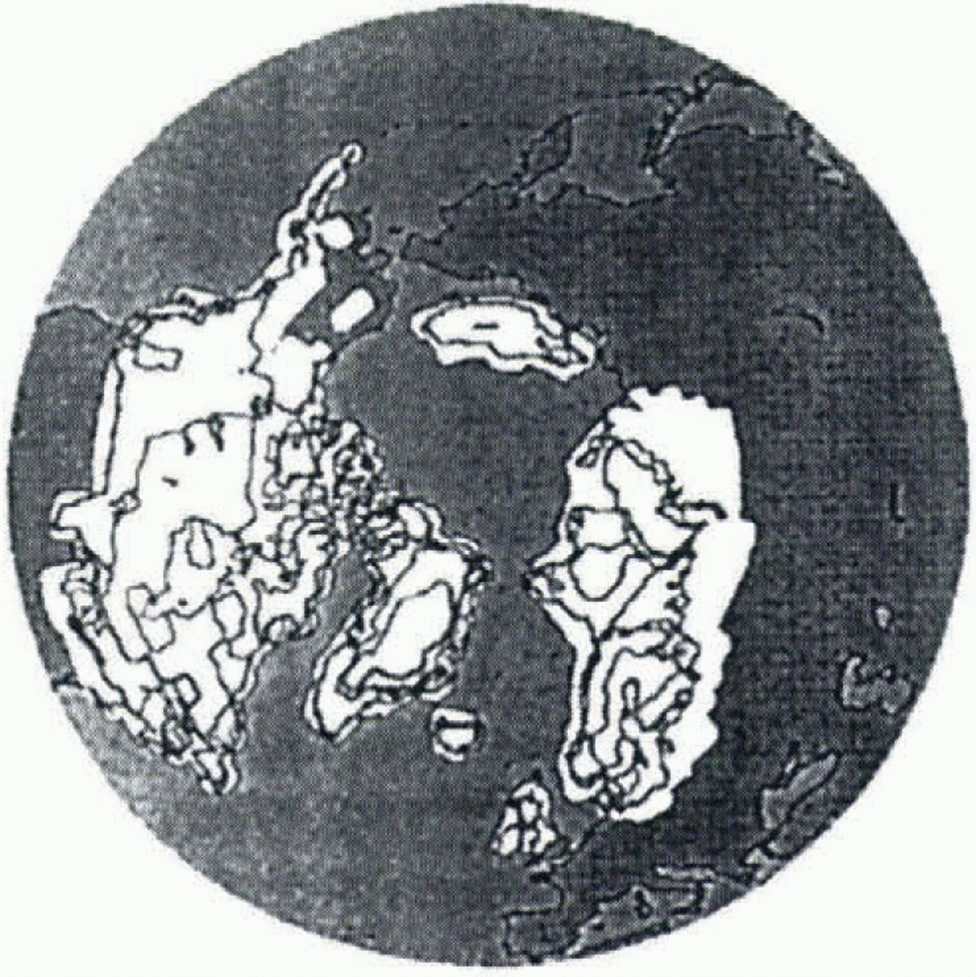
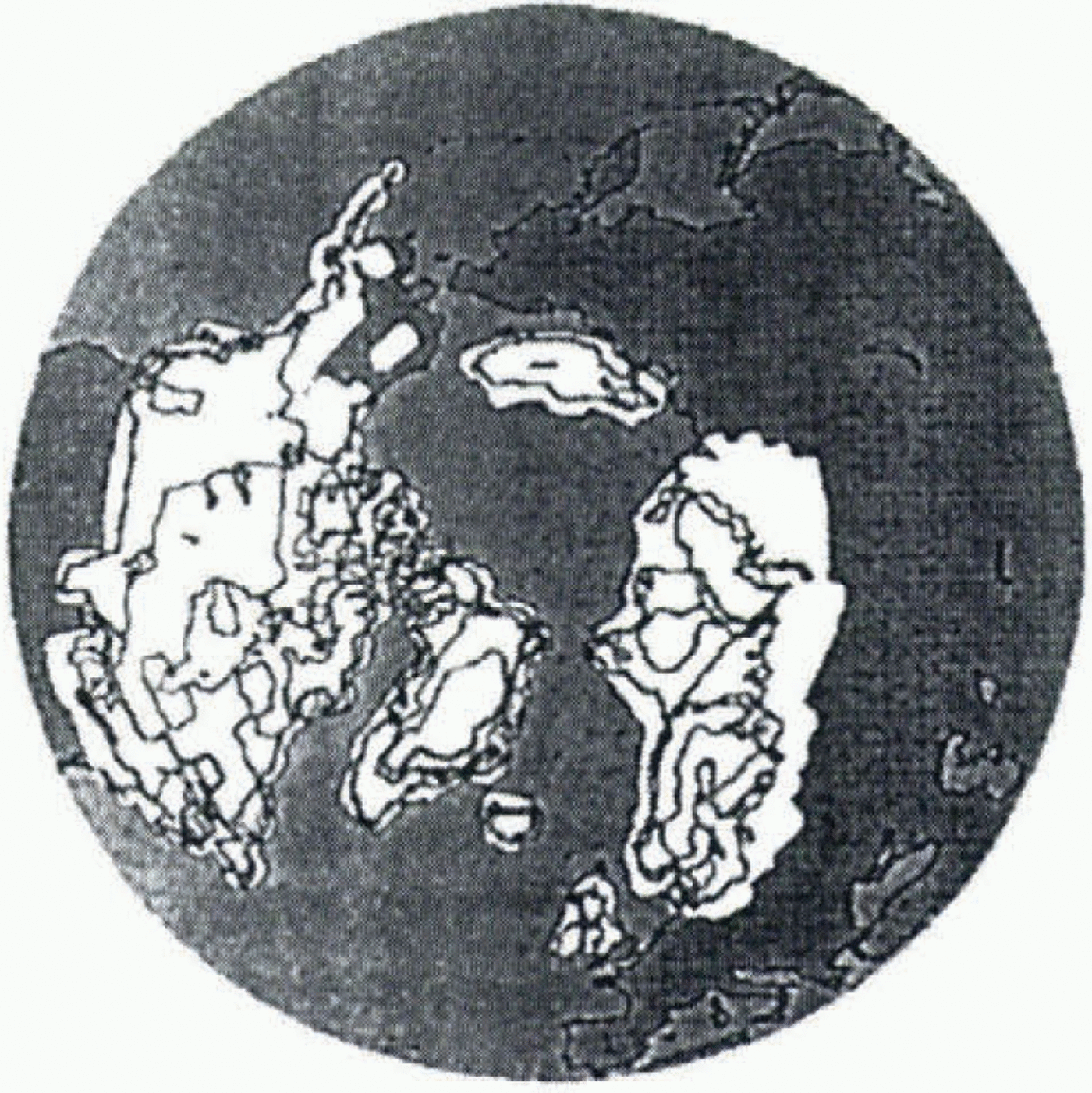
It is now commonly accepted that large ice sheets existed during the Last Glacial Maximum (LGM; 21 000 BP). The geological work which has been done up to now permits reconstruction of the maximum extent of the two main ice sheets, the Fennoscandian (over Scandinavia) and the Laurentide (over North America). The most recent reconstruction uses global rebound rates in a visco-elastic inverse model of the Earth’s crust (Peltier, 1994; Fig. 1). Modelling experiments have previously been done to simulate the ice-age cycle, by asynchronously coupling a climate model to an ice-sheet model, and comparing the modelled to the geologically reconstructed ice-sheet geometry. Marsiat (1994) couples a latitude–longitude vertically integrated ice-sheet model with a zonally averaged climate model, but the zonally averaged character of the atmospheric forcing leads to an ice distribution at the LGM that is different from the geological reconstructions. DeBlonde and Peltier (1991) couple a two-dimensional ice-sheet model with an energy-balance model, to simulate the evolution of the Laurentide and Fennoscandian ice sheets during the last glacial–inter-glacial cycle. They obtain satisfactory results, but their domain is restricted to these two ice sheets.

In this work, we focus on steady-state simulations of the present and LGM climate states. We use a three-dimensional thermomechanical icc-sheet model, developed at the Laboratoire de Glaciologie et de Géophysique de l’Environnement and already described by Ritz and others (1996). The model is forced with glacial climatic surface conditions to reconstruct LGM ice sheets, which we compare to Peltier’s reconstruction. We run the model until it reaches equilibrium, generally after 20 000–30 000 years. This is not entirely realistic, as present or LGM ice sheets are not

Fig. 1.

Reconstruction of the Northern Hemisphere ice sheets, using geological data, and a gravitationally self-consistent model for the computation of postglacial relative sea-level change; map copied from Peltier (1994).

in equilibrium. But, as we are chiefly interested in the spatial distribution of the ice, we consider that this assumption is not too restrictive.

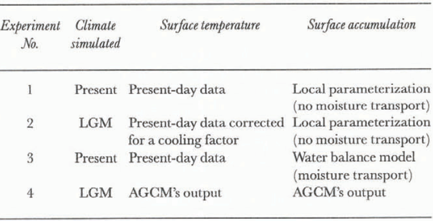
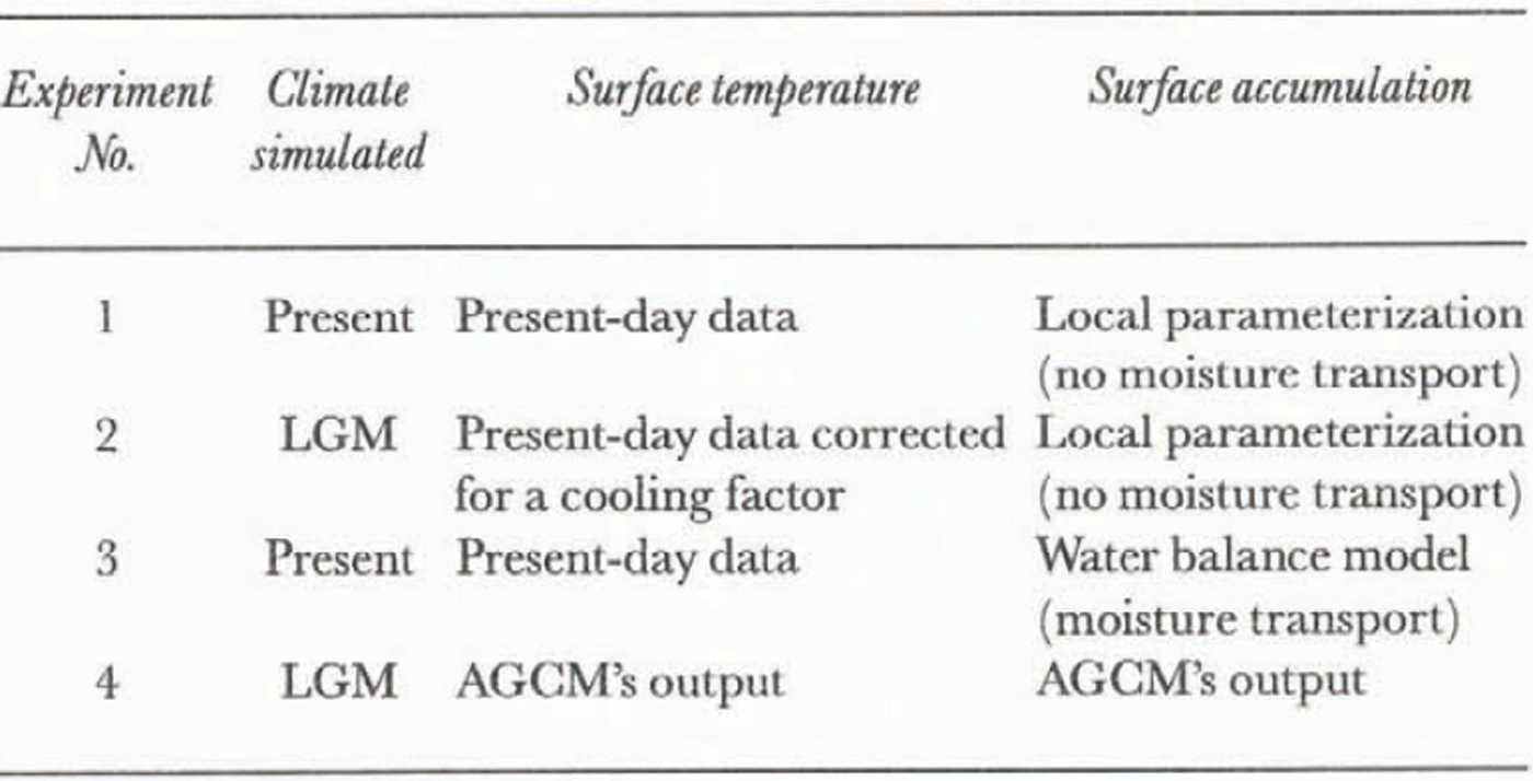
The ice-sheet model was first tested on the Greenland ice sheet (Fabre and others, 1995). One result of that study was to illustrate the high sensitivity of the model to the accumulation parameterization. The aim of the present work is to extend the model to the entire Northern Hemisphere and to test three different ways of computing accumulation and surface temperature. We first test the model with a local accumulation parameterization, using present-day climatic conditions corrected for a cooling factor, to simulate the LGM climatic conditions. Secondly, we use a more realistic accumulation parameterization by means of a water-balance equation, with the same initial climatic conditions as before. Finally, as these two methods do not give satisfactory results, we use as input to the ice-sheet model the results of LGM simulations of the LMD5 atmospheric global circulation model (AGGM), to compute accumulation. The experiments performed in this work are summarised in Table 1.

Table. 1.

Experiments performed in this work with the ice-sheet model

Ice-Sheet Model

Our model is a three-dimensional, thermomechanically coupled ice-sheet model. It takes into account the coupling between the temperature and velocity fields, and belongs to the same category as the models of Huybrechts and others (1991) and Greve and Hutter (1995).

The evolution of the ice-sheet surface and geometry is a function of surface mass-balance, velocity and temperature fields, and bedrock position. We will not present the main equations of the model, which have been described in Ritz and others (1996). However, we need to devote a few words to the mass-balance calculation.

Mass balance comprises four terms computed separately: accumulation, ablation, calving and melting at the bottom of the ice sheet. The accumulation treatment is a key factor, and will be developed further on.

Ablation is computed using the “positive degree day” method (Reeh, 1991), which uses the number of days with a positive mean temperature in an empirically derived function. It allows, by means of a Gaussian temperature distribution, some melting even on days when the mean temperature is slightly negative, since during the day the temperature may have been positive. Mean daily temperature is computed from the mean annual temperature, assuming that the annual temperature cycle can be represented by a sinusoidal cycle, with a maximum amplitude determined by the warmest mean monthly temperature.

As the surface temperature is dependent on altitude, it is computed each time the altitude has a new value, using a temperature vs altitude gradient of 8∘C km^–1, as is observed in the polar regions (Reeh, 1991).

There is no treatment of ice shelves in the model. Ice lost by calving at the margin is computed by setting the ice thickness to zero on a “coastline” determined by sea level. Sea level is set to zero for present state simulations, and to –105 m for LGM state simulations, following Peltier (1994).

The isostatic variation of the bedrock submitted to an evolving ice load is governed by two components: the flow of asthenosphere, treated with a characteristic time constant of 3000 years, and the rigidity of lithosphere, which is taken into account by computing the spatial shape of the deflection due to one unit load with a Kelvin function of zero order (Brotchie and Silvester, 1969), and by adding contributions of all the grid points covered by ice.

Various data are used as input to the model; topography, mean annual and summer surface temperatures and mean annual precipitation come from the U.S. National Oceanic and Atmospheric Administration (NOAA)/Environmental Protection Agency database (1990), with a resolution of 0.5∘ in longitude and latitude. On the Greenland ice sheet, where the database only provides ice-surface elevation, we use data compiled by Letréguilly and others (1991) for ice-surface and bedrock elevations, and we use surface temperature and precipitation from Ohmura and Reeh (1991), which are more accurate than the NOAA data in Greenland. Wind data are taken from the European Centre for Medium-Range Weather Forecasts database (Schubert and others, 1990); we use the two horizontal components (east–west and north–south).

These data, originally defined in longitude and latitude, are converted to a cartesian system by means of the Lorgna projection (Lambert azimuthal equi-areal projection), and interpolated by spherical interpolation on a 50 km x 50 km grid applied to the Northern Hemisphere. This grid (231 x 241 points) is the ice-sheet model’s grid.

Local Temperature-Controlled Accumulation

In the first two experiments we treat precipitation as a function of surface temperature, through the water-vapour pressure. Accumulation in each grid point is given by:

(1)

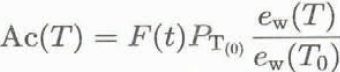
where T is the surface temperature, T ₀ is the surface temperature at present, PT ₍₀₎ is the precipitation at present, e _w is the water-vapour pressure, and F(t) is the fraction of the year with a mean temperature less than 2∘C, accounting for the fact that precipitation falls as snow for temperatures less than 2∘C (Letréguilly and Ritz, 1993).

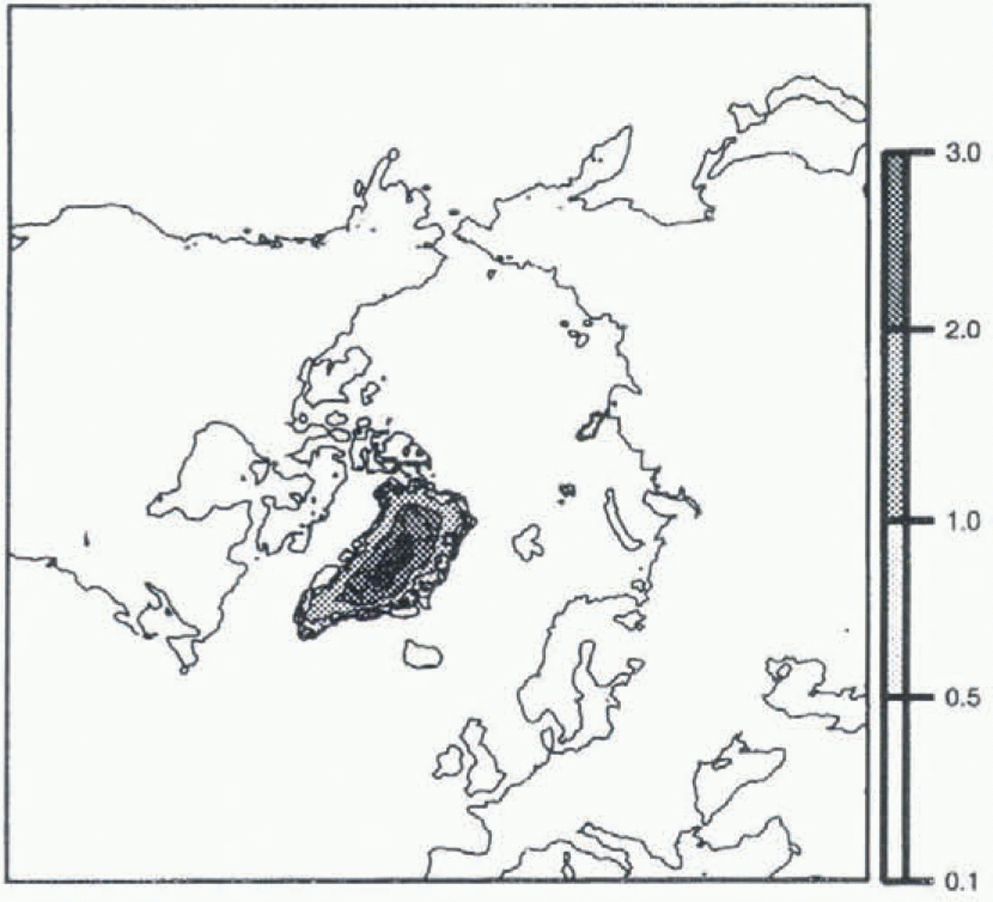
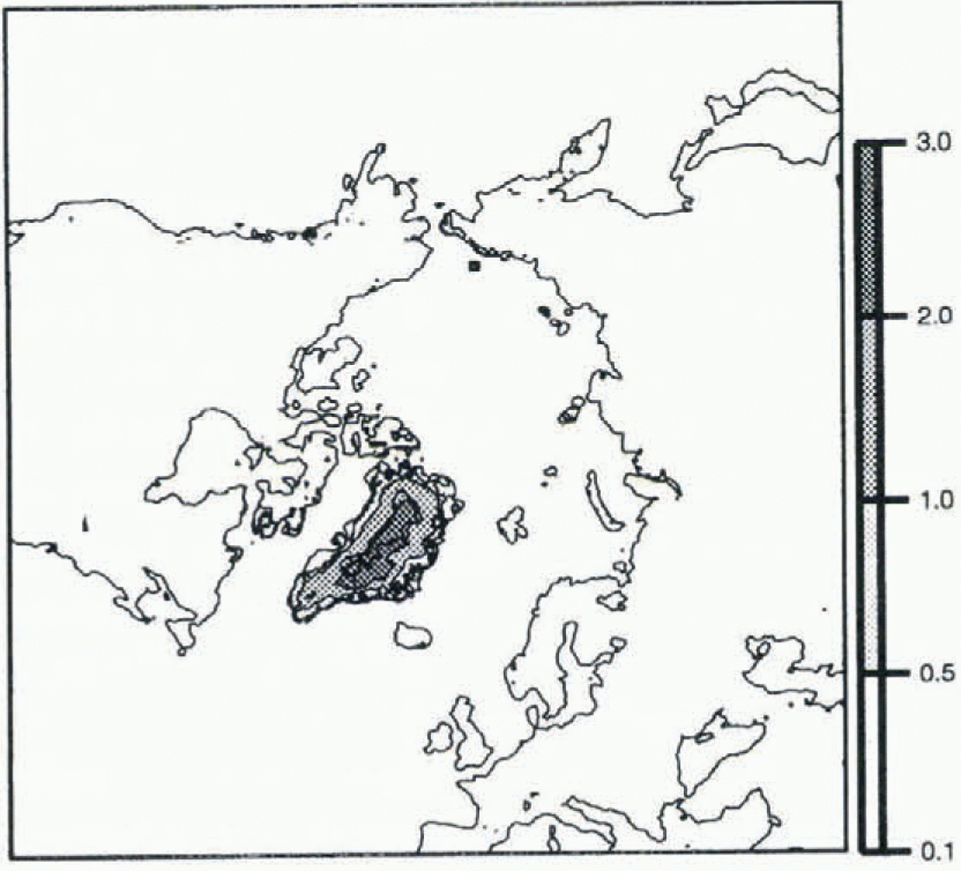
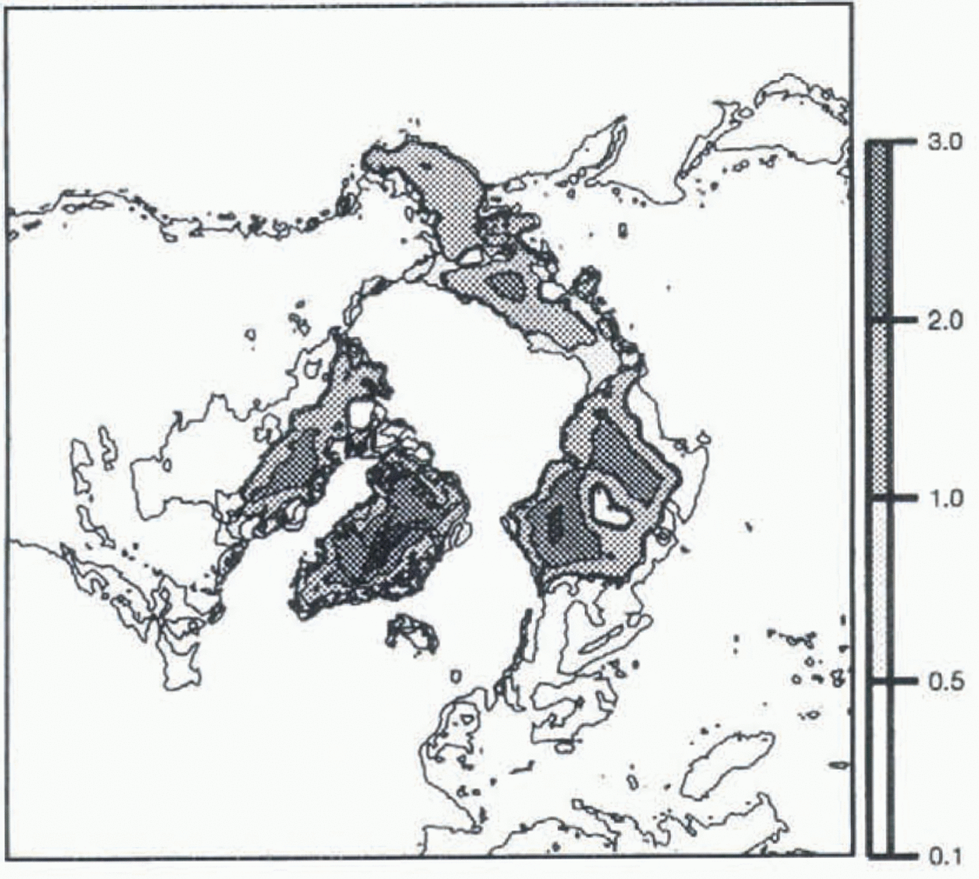
In experiment 1 we simulate the present state. Steady state was obtained after a 20 000 year run using the present climate (Fig. 2). The resultant ice-sheet geometry is in quite good agreement with the present ice distribution: the Greenland ice sheet remains ice-covered, with a maximum height (above 3000 m) and an extent close to today’s. There are even small ice masses on Svalbard, Iceland and Franz Josef Land, Russia. However, we produce no ice in Scandinavia, where there is some ice at present. This is not surprising, as the model grid (50 km) is too large to reproduce small features. While these results are satisfactory, we are aware that the present state is not in steady state, so that the simulation is not entirely realistic.

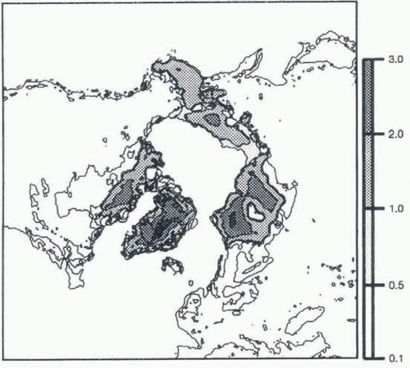
In experiment 2, we simulate the glacial state, by prescribing a cooling of 10∘C to the present surface temperatures. Again we run the model until it reaches equilibrium (20 000 years). When results of this simulation (Fig. 3) are compared with Peltier’s reconstruction (Fig. 1), we see that the ice is not extensive enough for the Laurentian and Fennoscandian ice sheets, and that global ice thicknesses are too low. The lack of ice can be explained by the absence

Fig. 2.

Map of the steady state obtained for Ihe present state, with the present climatology, and the local accumulation parameterization. Ice elevation isolines are in km. The thin line represents the land above sea level.

of moisture transport from the oceans inland in the accumulation parameterization scheme. Thus, water evaporated above the ocean cannot precipitate on land, and there is not enough moisture inland to form and maintain ice sheets.

Experiment 2 consists of two simulations, one starting with the present topography, and one with the glacial topography given by Peltier (Fig. 1), which give similar results. Thus, even when starting with the Laurentian and Fenno-scandian ice sheets, we are unable to maintain them, and, moreover, we form ice where geological data tell us there was none (on Alaska and Siberia). This method has also been used by Huybrechts and T’siobbel (1994) to reconstruct Northern Hemisphere ice sheets, and they also formed ice caps in Alaska and Siberia. It is therefore obvious that this accumulation parameterization is too crude to be able to simulate glacial states.

Moisture Transport

To simulate more realistic precipitations, especially for glacial conditions, we now use a more physically based precipitation

Fig. 3.

Map of the LGM steady state, obtained with the present climatology corrected for a cooling factor, and the local accumulation parameterization (no moisture transport).

algorithm, which permits moisture transport across grid points.

This method is based upon atmospheric water balance. It was developed by Sanberg and Oerlemans (1983), and was used successfully in a simulation of the Fennoscandian ice sheet (Letréguilly and Ritz, 1993). The variation with time of water content w in a vertically averaged atmospheric column is given by:

(2)

where S _L is related to the slope of the surface (when the surface is exposed to the wind, S _L is equal to the surface slope, otherwise S _L is equal to zero), v is the wind velocity, f ₀ is a background precipitation term, f ₁ is an orographical precipitation term, w _m is the maximum moisture contained in a vertically averaged atmospheric column, T _evap is the time needed to reach saturation in this column, and D _w is the moisture diffusivity. Values of w are obtained by solving Equation (2) with a finite-difference scheme on the grid previously described. In order to obtain w at equilibrium, iterations are made until steady values are reached.

Moisture balance is then governed by four terms, moisture advected by wind, precipitation, evaporation and atmospheric diffusion. The precipitation at time t and at a given grid point is given by the second term, and accumulation is obtained by considering only solid precipitation, and converting it to ice-equivalent thickness.

This model is of interest mainly because it takes into account the influence of topography on precipitation. This is particularly important in our simulations, where topography can vary from no ice to thousands of meters of ice (Laurentide at the LGM, for instance).

We have made sensitivity studies with the precipitation model to calibrate it to present-day precipitation. This must be done before we couple both models. We had the possibility of testing three parameters to obtain a best fit to present precipitation: we tested the influences of the height at which wind velocities are used as input to the model, of sea-ice extent and of variations in f ₀ and f ₁. The model is not sensitive to wind height, so we present only the results of the sensitivity tests to sea ice extent and f ₀ and f ₁.

Sea-ice extent influences the evaporation time T _evap; the time needed to reach saturation is much larger over ice than over sea, where evaporation is high. Therefore, different values are used for T _evap, depending on the nature of the surface. We tested two cases: no sea ice (leading to large values of evaporation in the high latitudes), and sea ice down to a fixed latitude (assumed to be the southern limit of the mean annual sea-ice cover, derived from Parkinson and others (1987). Not surprisingly, precipitation obtained with no sea ice is too high in the polar regions. When taking sea ice into account, we get a precipitation pattern closer to the present.

The remaining variables are the free parameters f ₀ and f ₁ used to calibrate the model to present-day values; they have a direct influence on the precipitation field in Equation (2). They do not vary spatially, which means there is only one value each of f ₀ and f ₁ for the whole domain. We started with values which were used in the Fennoscandian study, and, as we did not succeed in simulating present precipitation for the entire Northern Hemisphere, we tried to allow f ₀ and f ₁ to vary. It turns out that we did not find values giving satisfactory results. When the calibration seemed to fit the data in one area, it failed in another. In particular, we observed a lack of precipitation in central Greenland. This led us to think that processes governing precipitation on the Greenland ice sheet might be different from those in other areas, and that the precipitation algorithm is unsuitable for application to the entire Northern Hemisphere.

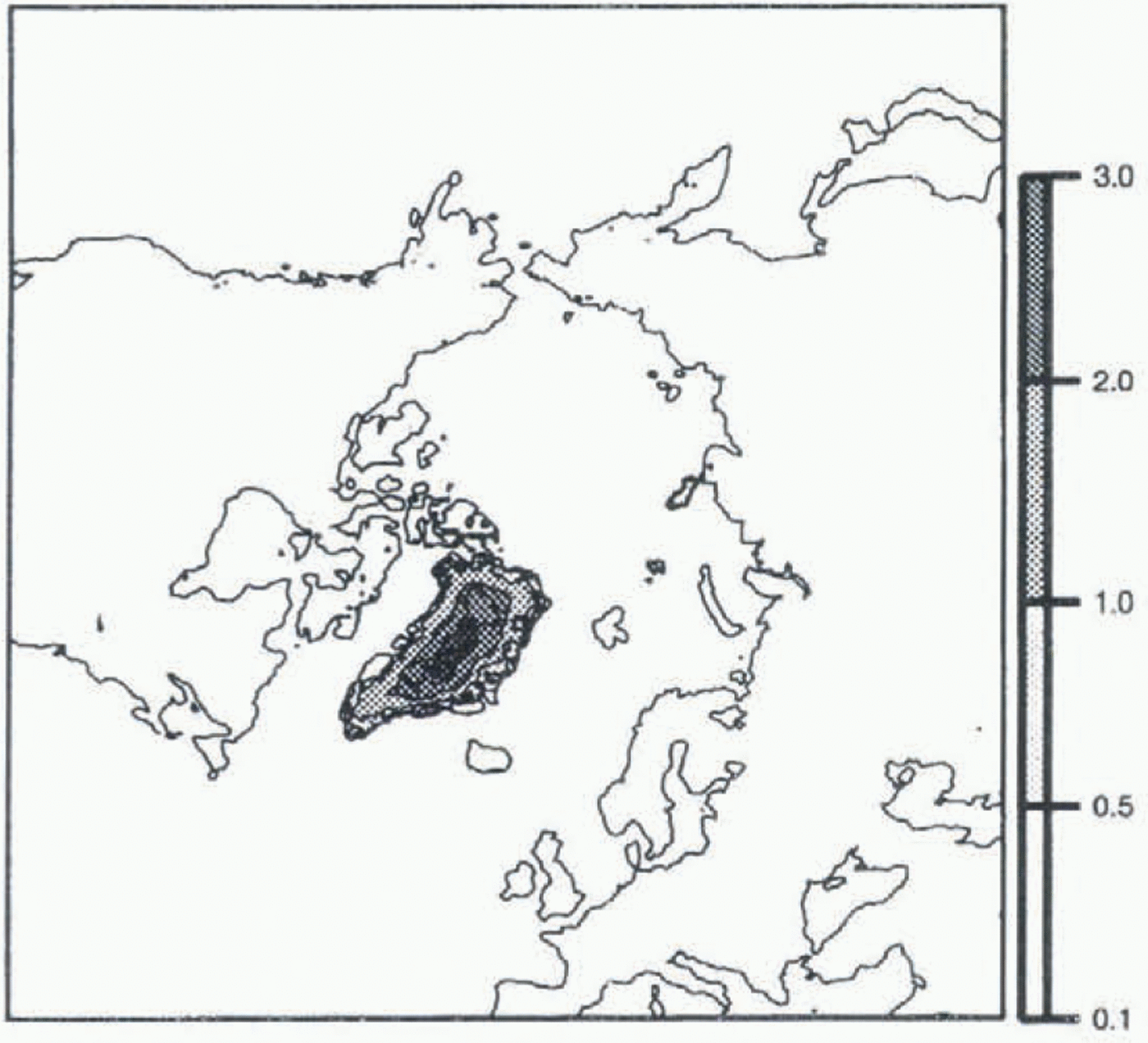
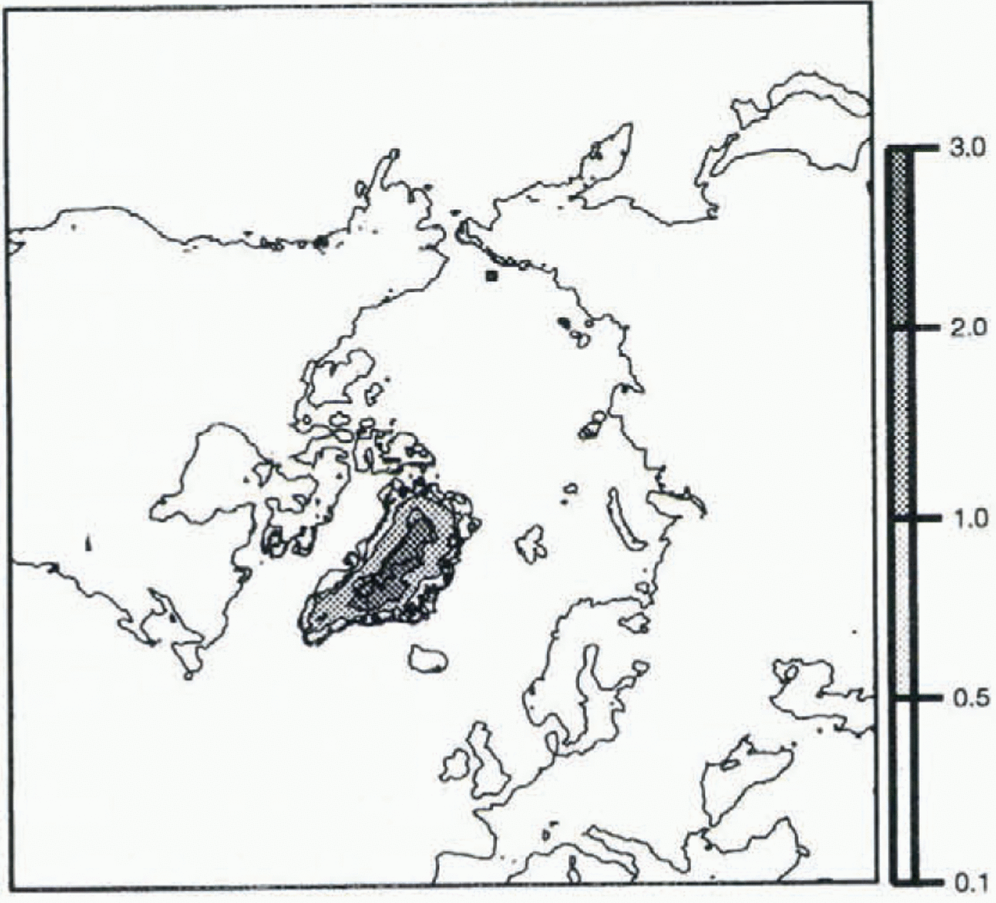
While aware of these unsatisfactory results, we have nevertheless tried to simulate the present state by coupling the precipitation and ice-sheet models. Results of experiment 3 show that the Greenland ice sheet is not high enough (Fig. 4); there is simply not enough accumulation to maintain the ice sheet at its present state. As we were not able to simulate even the present state correctly, it seemed to us that a glacial simulation would be meaningless.

Fig. 4.

Map of the present steady state, obtained with the present climatology, and the water-balance algorithm for the accumulation parameterization (moisture transport).

Coupled Agcm

The main result so far is that trying to simulate glacial states with the present precipitation as an input to the ice-sheet model, using only a temperature correction, is unrealistic, even when using a more physically based precipitation model. Thus we decided to use the outputs of an AGCM as input to the ice-sheet model.

The data used in this experiment come from the LMD5 AGCM, developed at the Laboratoire de Météorologie Dynamique (Sadourny and Laval, 1984) and used at the Laboratoire de Modélisation du Climat et de l’Environnement. The equations of the model are solved on a grid of 64 points regularly spaced in longitude (resolution of 5.625∘), and 50 points regularly spaced in sine of latitude (which means higher resolution near the equator, but lower resolution in the polar regions). The model has ll layers in the normalized pressure coordinate: four layers in the planetary boundary layer, four in the free troposphere and three in the stratosphere. It is based on mass continuity, water-vapour conservation and the dynamic and thermodynamic equations. The LGM LMD5 simulations are performed with the following boundary conditions: 200 ppm of C02 (instead of 345 ppm for the present), an initial glacial topography given by Peltier’s reconstruction (interpolated on the AGCM grid), and sea surface temperatures prescribed by the CLIMAP database (1981). These conditions are those required in the PMIP program (Joussaume and Taylor, 1995), which aims to provide an intercomparison of the results of different atmospheric circulation models, prescribing the same boundary conditions, for two palaeo-climatic states, including the LGM. In this work we use prescribed (sea surface temperature) SST changes; in a later work we will use an interactive surface ocean.

The initial topography for the LGM simulation comes from Peltier (1994). Surface elevation (resolution 1∘ X 1∘) is interpolated on the ice-sheet model’s 50 km x 50 km grid. As we need to input bedrock topography and ice thickness in the ice-sheet model, and we only have at our disposal surface elevation, we compute these fields from the surface altitude in a very simple way, by assuming that the ice load leads to a bedrock-lowering equivalent to one-third of the ice thickness. This crude assumption is used only to start the simulation; isostasy is computed afterwards in the ice-sheet model in a more realistic way, as described earlier.

We use three data sets from AGCM simulations of the LGM and the present as inputs to the ice-sheet model: mean annual surface temperature, mean annual precipitation and mean JJA (June, July, August) surface temperature. Mean annual precipitation and temperature are used to compute accumulation, and both temperatures are used to compute ablation. These data are converted from the AGCM grid to our cartesian system by the Lorgna projection, and interpolated on the ice-sheet model grid.

Methodology of the coupling

In order to simulate a glacial state with the ice-sheet model, we want input data representative of a glacial climate. S. Joussaume (personal communication, 1996) has suggested that anomaly fields (i.e. differences between control and LGM climates) simulated by the AGCM are more representative than direct control or LGM fields. Thus, if we consider a variable X, LGM data are given by:

(3)

where X _{LGM AGCM} – X _{present AGCM} is the anomaly in output of the AGCM, and X _present is the present-day observed value (data set used in the first two experiments of this work). This was done first for the temperature fields.

The computation of LGM temperatures must take into account the correction of temperature for altitude. The anomaly data and the topography, both on different grids, are interpolated on to the ice-sheet model grid. Temperatures need to be computed again at the altitude of each grid point of the ice-sheet model, since each value of the anomaly is given at the altitude of the corresponding grid point of the AGCM. This correction is performed using the same gradient of temperature for altitude (8∘C km^–1) as in the ice-sheet model. The new temperature at a given grid point is then:

(4)

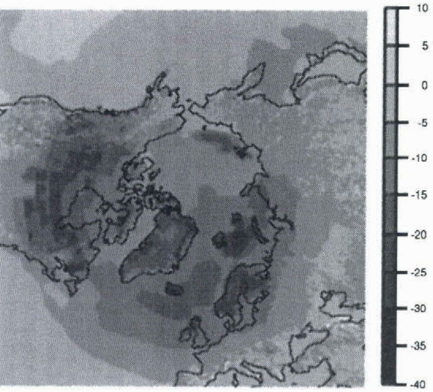
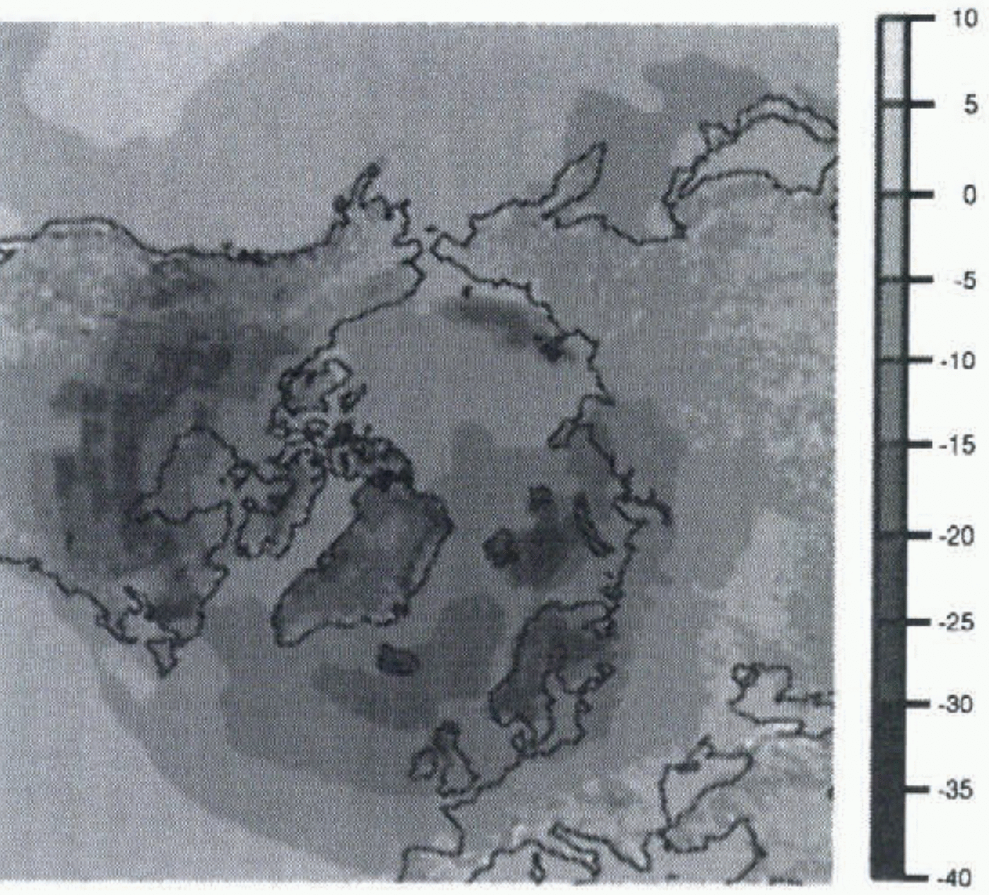
where alt _new is the altitude given by Peltier’s topography interpolated to the ice-sheet model grid, and alt _old is the altitude given by the topography used in the AGCM, interpolated to the ice-sheet model grid. Figure 5 shows the difference between mean annual surface temperatures obtained for the present and for the LGM. The correction allows a more precise topography to be taken into account, especially in regions such as Greenland where the AGCM has a low resolution. With this low resolution, the surface is greatly smoothed at high latitudes. Thus, by coupling asynchronously the AGCM and the ice-sheet model, we are able

Fig. 5.

Map of the difference between mean annual surface temperature for the LGM and the present, in ∘C. This difference is an output of the AGCM; it is used to compute LGM surface temperatures which are an input to the ice-sheet model.

to use fields which are available only as AGCM outputs, and to compensate for the low resolution of the AGCM by correcting these fields on the finer grid of the ice-sheet model.

We did not correct the precipitation in the same way, because it is not a direct function of the altitude and is therefore more difficult to correct. However, precipitation is also influenced by topography. We reconstructed precipitation by the same method of anomalies. In some places the anomaly was larger than present-day data, resulting in negative precipitation during the LGM! To avoid this problem, we use a ratio of precipitation rather than a difference:

(5)

Equation (5) seems to be physically more convenient than the previous method of computing precipitation. We can indeed consider that a large part of the precipitation variations can be related to the water-vapour pressure-content variations in the air (as in the first experiment). As saturation water-vapour pressure is an exponential function of

Fig. 6.

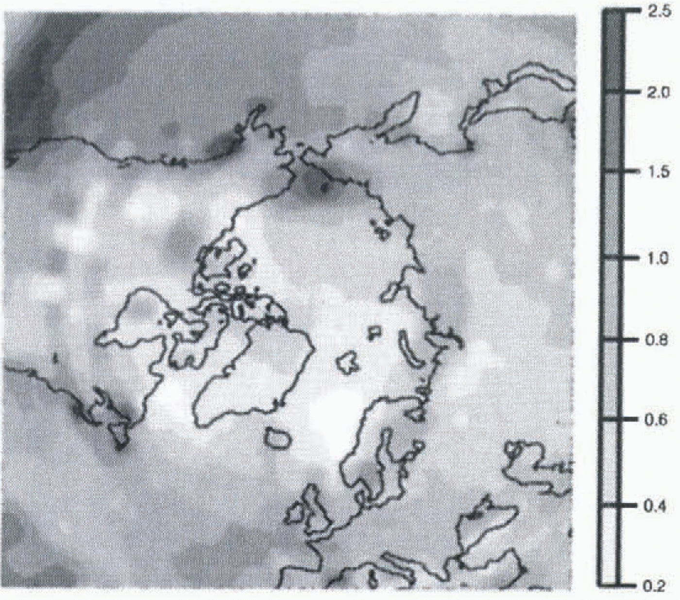
Map of the ratio of precipitation between LGM and present, in m year^–1. This ratio is an output of the AGCM; it is used to compute LGM precipitation which is an input to the ice-sheet model.

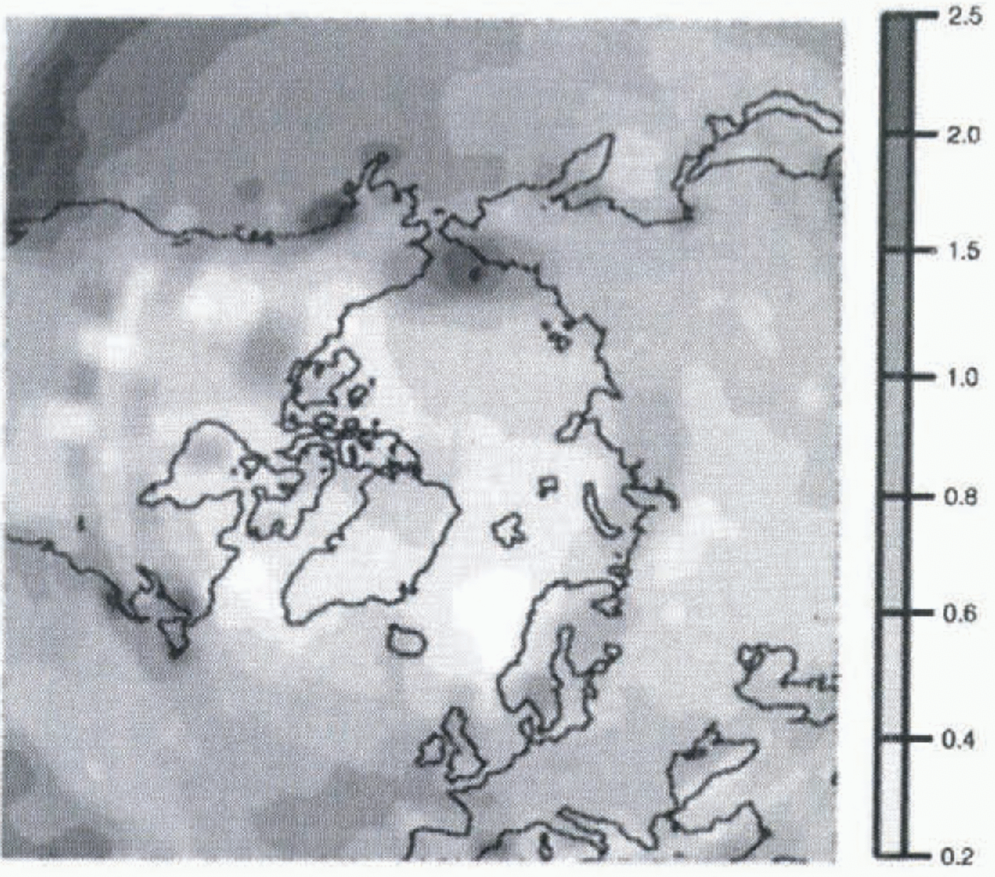
temperature, a temperature variation in terms of a difference will lead to a precipitation variation in terms of a ratio. The ratio of precipitations obtained between present day and LGM is shown in Figure 6. We observe lower values for the LGM than for the present, as can be expected for a glacial climate, with colder air containing less precipitable water.

Results of the coupling

We simulate the LGM slate by running the ice-sheet model until it reaches equilibrium, approximately 30 000 years, using the data discussed above and Peltier’s glacial topography as initial conditions.

In the LMD5 AGCM simulations we use, the SSTs are prescribed by the CLIMAP dataset. Thus there is no possibility of evolving temperatures on sea grid points, as there is on land grid points. This creates large temperature contrasts from one grid point to another in coastal regions, and leads to less realistic temperature maps. In experiment 4 we use T ^air, the air temperature 10 m above ground, instead of

Fig. 7.

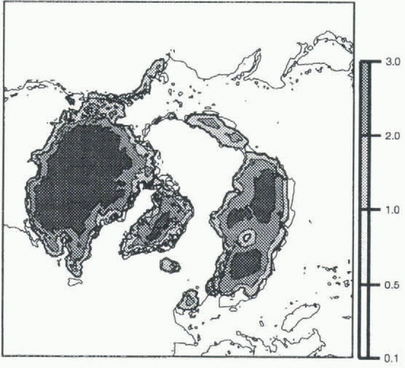
Map of the LGM steady state, obtained with the LGM data in input (reconstructed from the LMD5 AGCM outputs). The thin line represents the land above sea level, 105 m lower than in Figure 2. T _ground. The mixing of air which occurs at a height of 10 m leads to a more representative temperature here than on the ground, even though T _air is globally slightly warmer than T _ground.

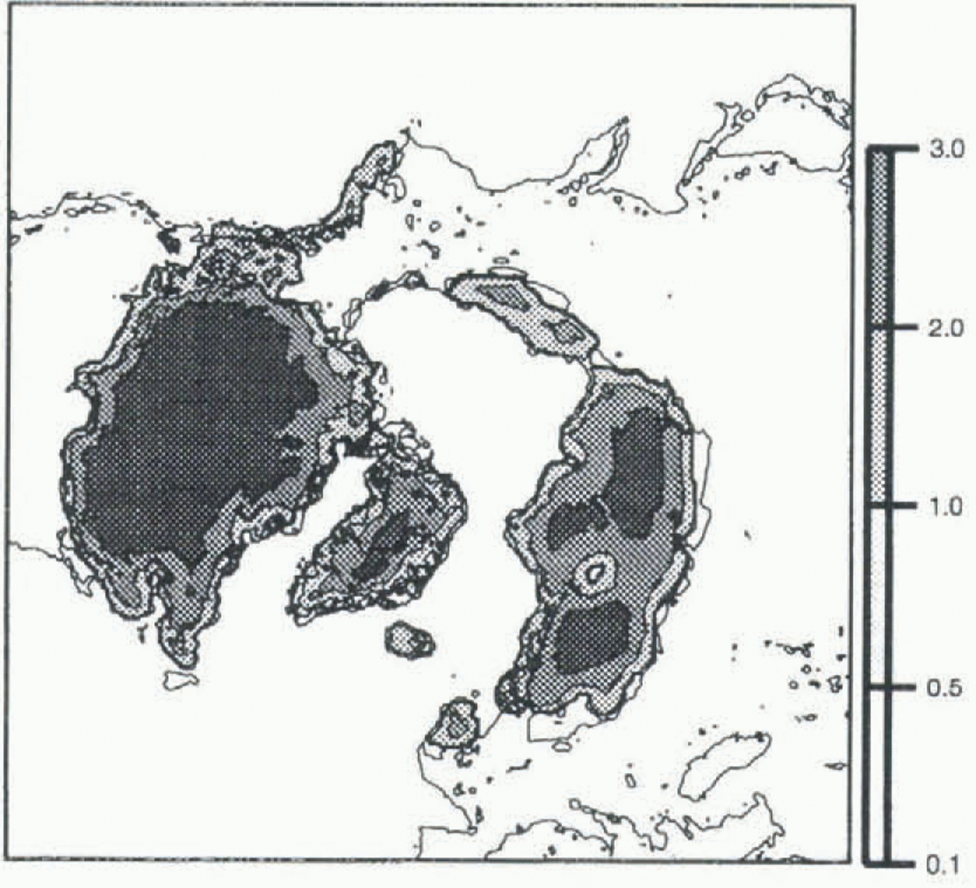
Results obtained with T _air are presented in Figure 7. It is obvious that they are in much better agreement with geological reconstruction (see Fig. 1) than the results we obtained in the first part of the work. We succeed in maintaining ice on North America and Scandinavia, for example, and Alaska and Siberia are not ice-covered: the two latter regions are of particular interest, because geological data tell us they were not covered with ice at the LGM, and most “coupled” atmospheric–ice-sheet models predict ice. This satisfactory result is probably due to the outputs of the AGCM rather than to a particular feature of the ice-sheet model. On the other hand, the Greenland ice sheet is very low (down to 2500 m) compared to the present ice sheet. Although accumulation is reduced in a glacial climate, such a pronounced decrease of the ice sheet seems unrealistic.

The decrease may be due to the low resolution of the AGCM at high latitudes. As precipitation was not corrected for altitude, we could have smaller values in Greenland than we would get with better resolution. One can also observe a deflection in the middle of the Fennoscandian ice sheet. This feature disappeared when we tried a simulation using T _ground instead of T _air, but other problems appeared when using T _ground, due to the prescribed SSTs. This makes us think that the deflection in the Fennoscandian ice sheet is due to too warm an air temperature at this point. We hope to obtain better results when data from the AGCM simulation using evolving SSTs become available.

Conclusion

Experiments 1–3, which use simple precipitation algorithms to parameterize accumulation during the LGM, give dubious results. Furthermore, we are not even able to reconstruct present precipitation distribution in the Northern Hemisphere with the water-balance equation. Our conclusion is that the processes governing precipitation can vary greatly from place to place, and that it is therefore difficult to model precipitation without including all the processes involved. Thus, the best way to input realistic LGM climatic data to an ice-sheet model to simulate the LGM state is to use AGCM outputs.

In this work we used the results of simulations of the LMD5 AGCM to run the ice-sheet model. The ice distribution we obtain for the LGM is very close to Peltier’s reconstruction. In particular, Alaska and Siberia remain ice-free, and the Laurentian and Fennoscandian ice sheets have the correct extent and thickness.

In future, we intend to study the influence of the AGCM resolution on the ice-sheet model results. To this end we will couple the ice-sheet model with the previous version of the LMD AGCM, which has an even lower resolution. We will also study the influence of the initial topography on the results, by using outputs of LMD simulations starting with two different ice repartitions (CLIMAP and Peltier). And finally, we intend to use outputs of other AGCMs with a better resolution in the polar areas.