1. INTRODUCTION
It is well known that the properties, particularly the power, of unit root tests depend upon the trending characteristics of the deterministic component in the maintained model. Numerical and asymptotic evidence of this is contained in Perron (1989), DeJong, Nankervis, Savin, and Whiteman (1992), Zivot and Andrews (1992), and Leybourne, Mills, and Newbold (1998).
Analysis of this dependence appears in Durlauf and Phillips (1988), Phillips (1998), and Ploberger and Phillips (2002, 2003) with derived asymptotic relationships between nonstationary processes and deterministic trends. The first two papers concern the spurious success of regressions of unit root processes on linear trends and vice versa. The latter two demonstrate that our ability to model nonstationary series is limited by both the number and trending characteristics of deterministic components.
Despite this body of evidence a precise relationship between a unit root process and a simple linear trend has not yet been detailed. This paper provides such a relationship in the context of invariant unit root tests. The available information for such tests is defined to be Fisher information in the maximal invariant, of which all invariant tests must be functions; see Lehmann (1997). For the Sargan and Bhargava (1983) formulation it is found that requirement of invariance with respect to a linear trend implies that the available information is zero at the unit root. This result holds over a family of sample distributions, for any additional deterministic components, for any sample size, and for a general class of innovation dependence.
For the simple zero-mean Gaussian AR(1) process it is well known that the standardized observed information converges to a random variable. Moreover, for potentially nonergodic processes we do not have uniform convergence of estimators over the parameter space, nor are asymptotic distributions Gaussian. Consequently, the role of Fisher–Rao efficiency theory, having Fisher information at its heart, is at best ambiguous. Despite this, this paper is able to demonstrate a central role for information in determining the properties of tests.
It is shown that the power of any invariant test will be bounded above by the chosen size plus a simple function of the available information. Consequently, the relationship between the efficiency of a test (power minus size) and information is preserved and applies generally. In addition, as a corollary to the main theorem, it is demonstrated, via an applicable bound fundamental to the Fisher–Rao theory, that the variance of any trend invariant test is indeterminate, under a unit root.
The majority of asymptotic treatments of unit root testing adopt a local-to-unity framework, for example, that of Phillips (1987) and Elliott, Rothenberg, and Stock (1996). Supposing that the autoregressive parameter is in an asymptotic neighborhood of one, say, 1 − O(cN), where cN → 0 as the sample size N → ∞, then this paper finds that the information is of order O(N2) in that neighborhood. On the other hand, if cN is O(1), the model trend is stationary, and information is of order O(N).
The results of this paper help explain two key findings within the literature: that the inclusion of trends has a detrimental effect on the power of tests in general and that this is specifically acute for locally most powerful tests. These findings are neatly illustrated by the numerical work of Dufour and King (1991) and Elliott et al. (1996). Following Rao (1945), Fisher information may be interpreted as a metric on the space of densities. Furthermore, Efron (1975) and Kallenberg (1981) argue that high curvature, which is inversely proportional to information, implies a lack of efficiency for linear methods, such as locally most powerful tests.
There has been much success in terms of characterizing the asymptotic distribution of unit root tests. Despite this success, excepting the simplest zero-mean AR(1) case, as in Abadir (1993), we have no analytic expressions for asymptotic moments, densities, or distributions. Without such expressions, establishing results analogous to those derived here would prove impossible. Consequently, our only knowledge of the influence of trends on, for example, the power of unit root tests comes from Monte Carlo experimentation. This paper provides an explicit link between the inclusion of a trend, its impact upon information, and thence the power of any invariant test.
It does not follow from the results that linear trends should be excluded from deterministic components in the unit root context. Instead, this paper highlights the importance of determining the necessity of trends prior to the unit root test being performed. Tests for precisely this purpose have recently been constructed; see Vogelsang (1998) and Bunzel and Vogelsang (2003).
The plan for the rest of the paper is as follows. The next section details the model and the assumption under which the results hold and presents all of the results in a single theorem. Section 3 discusses the implication of these results, and Section 4 concludes. An Appendix contains the proof of the theorem and of a key lemma.
2. ASSUMPTIONS AND MAIN RESULTS
We will consider the formulation of the unit root hypothesis in the time series regression

In (1) β = (β1,β2,β3′)′ is a k × 1 vector of unknowns, zt a (k − 2) × 1 vector of strongly exogenous variables, and εt a zero-mean, stationary, and ergodic innovation sequence having covariances E [εtεs] = σ2ω(|t − s|). Regressions of this type were introduced by Sargan and Bhargava (1983) in the context of testing for a unit root. We shall consider hypothesis tests of

and in particular those tests that are, at least asymptotically, invariant with respect to the deterministic and exogenous components in (1) and the marginal variance of εt. Consistent, robust testing procedures for (2) in (1) are fully established within the literature; see, for example, Elliott et al. (1996). Asymptotically the resultant tests are invariant, and thus our results will have some bearing upon all of these procedures.
Let y = (y1,…, yN)′, ε = (ε1,…, εN)′, e = (1,1,…,1)′, τ = (1,2,…, N)′, Z = (z1,…, zN)′, X = (e : τ : Z) and let σ2Ω = E [εε′] be the covariance structure of the stationary innovation sequence. As a consequence (1) may be written as

where Tρ = IN − ρL(1) and L(1) is the N × N matrix lag operator, having ones on the first lower off-diagonal and zeros elsewhere.
We shall proceed under the following assumption on the density of y and the family

of which it is a member.
Assumption 1.
(a) Let the density of y, given Z, be

with

where X and β are defined following equations (2) and (1), respectively, σ2 is a scalar, and Ω is an N × N covariance matrix so that Σρ(Ω) = Tρ−1Ω(Tρ−1)′. Furthermore, we assume that q[.] is a nonincreasing convex function on [0,∞).
(b) Ω is such that (1) Σρ(Ω) depends on ρ for all

and (2)

, for all N.
It is presumed that the regressor set always includes a constant and a trend. However, the augmented regressor set may include additional polynomial trends or any random (exogenous) regressors to be conditioned upon. Assumptions on the initial condition that are consistent with Assumption 1 are either that it is constant (without loss of generality, zero) or that it is exogenously distributed and so may be conditioned upon and included in the regressor set. To illustrate how a nonzero initial condition, y0, can be incorporated, suppose there are no other regressors, so that

where y0 = (y0,0,…,0)′. That is, in terms of the notation of Assumption 1, Z = y0. Thus for the first two values of y,

and no other yi depends upon y0 explicitly. Although inference on β3 would not be possible in this setup, our inferences on ρ can be made invariant with respect to y0. Therefore inference upon ρ will not depend upon β3 in the sense that neither the size nor the power of any suitable test will depend upon this nuisance parameter.
Part (ii)(1) of Assumption 1 ensures that there are no common factors in the covariance structure of the data and so ρ may be identified, in principle. Part (ii)(2) guarantees the “finiteness” of Ω with respect to the absolute column sum norm. It implicitly provides for the ergodicity of the εt in that the columns/rows of Ω must be absolutely summable as N → ∞. Notice also that because ε is covariance stationary then Ω is Toeplitz.
Assumption 1 also implies that the data have a distribution within the family of elliptically symmetric distributions. This family includes all finite mixtures of normals, including multivariate t-distributions, with the Cauchy as a special case. That is, the kurtosis of the {yt} may be any constant not depending upon the parameters, although skewed distributions are ruled out.
To proceed define the N × N − k matrix C by

so that C is the singular value decomposition of MT1 X. Let w = C′T1 y and consider the group G = (a,g), with

and

and with action

then the maximal invariant, under G, for testing H0 in (2) is

see Kariya (1980) and King (1980). Furthermore the density of and Fisher information in the maximal invariant are given in the following lemma, which is proved in the Appendix.
LEMMA 1.
(i) The density of v on the surface of the unit N − k sphere, with respect to normalized Haar measure, is

where A = C′T1Σρ(Ω)T1′C.
(ii) The Fisher information in v about ρ is

where A is defined following (4), A = C′T1 [dρΣρ(Ω)]T1′C, and dρΣρ(Ω) denotes the derivative of Σρ(Ω) with respect to ρ.
To summarize: the density of v depends upon neither β nor σ2, nor, given Assumption 1, the distribution of the data. Thus the expression for Iv(ρ) does not depend on which member of the family

generates y. Generally, though, it will depend upon the structure of σ2Ω. We will thus refer to (5) as the available information for invariant tests, in the sense that any invariant test, or indeed any other function of the maximal invariant, will have Fisher information bounded above by this quantity.
On the basis of Lemma 1, we are able to demonstrate the following facts about information at and near the unit root. First, information vanishes at the point of unity; that is, the available information is zero at the unit root. For any other point information is nonzero and in any asymptotic neighborhood will grow as the square of the sample size. Asymptotic neighborhoods are of specific interest for unit root tests, and so we prove that the asymptotic power (minus size) of any invariant unit root test can be bounded above by a simple function of the available information and the radius of the asymptotic neighborhood. These results are contained in the following theorem, which is proved in the Appendix.
THEOREM 1.
(i) For all sample sizes N, for all sets of exogenous or fixed regressors Z, and for all Ω that satisfy Assumption 1(b), the Fisher information in v is zero at ρ = 1; that is,

(ii) Define any asymptotic neighborhood of the unit root by 1 − ρ = O(cN) > 0, with cN → 0 as N → ∞; then in that neighborhood,

(iii) Let

be the power of any invariant unit root test, of size δ, against the alternative with 1 − ρ = cN; then for some c* ∈ (0,cN),

3. DISCUSSION AND ANALYSIS
Theorem 1 demonstrates that the available information is zero at a unit root but generally nonzero in any asymptotic neighborhood. Moreover, an explicit relationship between the power of invariant tests is derived. In this section implications of the results will be discussed, in particular within the context of the inferential problem of testing for a unit root.
3.1. Available Information Is Zero at a Unit Root
The strongest result contained in Theorem 1 is that the information vanishes in model (3) at the unit root whenever a trend is included as a regressor. This result holds for all other sets of variables zt, including higher order polynomial trends, and for any Ω defined for a stationary error sequence. The crucial relationship that leads to all of the results in this paper is that the derivative of the autoregressive covariance matrix is matrix colinear with the outer product of the trend, namely,

where Σρ = Tρ−1(Tρ−1)′. Consequently, any projection of the derivative in the space orthogonal to a trend yields a covariance derivative at unity that is equal to minus the covariance. The properties of invariant unit root tests when a linear trend is included follow as a consequence of this relationship.
Formally this result holds only for the inclusion of a linear trend. However, it may be inferred that “trendlike” regressors will have a negative impact upon available information. This follows because the projection orthogonal to such regressors will be “close” to being orthogonal to τ and thus the quantity A−1A in (5) evaluated at the unit root will be “close” to the identity. Examples would be inclusion of structural breaks in the constant, periodic functions with long periods, or the inclusion of strongly trending exogenous variables.
Part (i) of Theorem 1 also points to another valuable prediction. The statistical curvature obtained by Efron (1975) is inversely proportional to the information, whereas Kallenberg (1981) argues that large curvature implies a shortcoming of locally most powerful tests. In the extreme case of the inclusion of τ as a regressor, curvature will be unbounded. Therefore, we would expect inclusion of trending regressors to have a significant negative impact upon the power of any locally most powerful testing procedures; indeed, see the numerical work contained in Forchini and Marsh (2000).
Later in this section we will discuss the information in an asymptotic neighborhood of one. Before getting there though it is worth pointing out that because Iv(ρ) is differentiable in ρ (in fact it is analytic in ρ, because Σ(ρ) is infinitely differentiable for every ρ), then we can find arbitrarily small and positive κ1 and κ2 so that

That is, information is vanishingly small in nonasymptotic neighborhoods of unity. In asymptotic neighborhoods the story is quite different, as is apparent from part (ii) of the theorem.
Suppose that we take the density in (4) as a likelihood for ρ and with a score given by

Then because Var[Sv(ρ)] = Iv(ρ) it follows that Sv(1) = 0 for all v. That is, the score is constant at the unit root. The fundamental implication of the score being constant is that the maximum likelihood estimator for ρ based upon (4) will not converge uniformly. However, because there is not uniform convergence in autoregression in any case, the additional results of Theorem 1 are needed to explore the consequences of this.
The fact that information is zero is preserved in two interesting special cases. First it is well known in the seasonal unit root literature that the trend (−1)tt is the analogue to the linear trend in the positive unit root case. If we call the maximal invariant for this case

, then one can establish that

, also. In addition, suppose that we quasi-difference the data, that is, take Tρ0 y, where Tρ0 = I − ρ0 L, ρ0 ≠ 1. Again calling the maximal invariant for this case v(ρ0), then also Iv(ρ0)(1) = 0. It therefore seems that it is only the requirement of invariance to a trend at the unit root that matters, not precisely how this is achieved.
3.2. Detrending and Differencing
That information is zero is a consequence of the algebraic identity given in (6). Related to that identity is a heuristic explanation as to why it is that the precise combination of a linear trend and unit root implies a complete loss of information.
There are two methods for trend removal: either one can project the data onto the space orthogonal to that trend, or one can difference the data. Suppose in a basic model with a constant and trend that we difference the data d times and obtain

then for any d a maximal invariant is defined by

However, notice that in (7) all we have really achieved is to transform the variance of y, under the null, to

and the identity in (6) then becomes

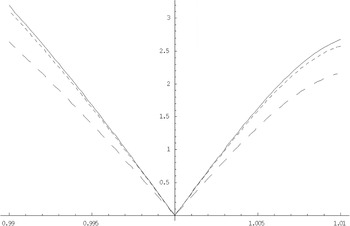
Furthermore, running through the proof of part (i) of Theorem 1 in the Appendix we find that an identical argument applies. That is, the common orthogonality of C(d)′ to both (T1)dτ and (T1)d(dΣρ /dρ)|ρ=1 gives exactly the same result. Thus, at the unit root, there is a synonymity between projecting out a trend and differencing it out. Moreover, this applies for differencing an arbitrary number of times. It is well known in the standard time series literature that differencing, particularly overdifferencing, destroys signal, or here, information. To illustrate this point Figure 1 plots Iv(d)(ρ), in a neighborhood of ρ = 1, for values of d = 1,3,6 for a sample size of N = 50. Clearly we lose information by differencing; ultimately as d → ∞ we would expect to lose all information. At the unit root, via (8), projecting out the trend is equivalent to differencing to this limit.

Plots of Iv(d)(ρ) based on model (7) for N = 50 and different d. Solid line: d = 1; dotted line: d = 3; and dashed line: d = 6.
3.3. Information and Fisher–Rao Efficiency
The general validity of the efficiency theory of Fisher–Rao is lost for problems in which there is not uniform convergence over the parameter space leading to non-Gaussian asymptotics. Indeed, for the pure random walk it is well known that the standardized observed information is random, although still having mean equal to the standardized expected information.
Despite that, absolute efficiency bounds may still be derived in the context of the current framework. Doing so yields an interesting corollary to Theorem 1. Let t(v) be any invariant statistic having finite mean τ whose derivative is also finite, that is,

Now construct a statistic

where Sv(ρ) is the score. Minimizing the variance of t*(a) with respect to a (the minimum occurs at a = (dτ/dρ)′Iv−1(ρ)) and noting that by definition Var[t*(a)] ≥ 0, it must be that

That is, the variance of any statistic t(v) has a lower bound involving Fisher information. For the unit root we obtain the following corollary.
COROLLARY 1. Let t(v) be any trend invariant unit root test or estimator having finite mean τ(ρ) with finite first derivative τ′(ρ) in the autoregressive parameter ρ; then the variance of t(v) is indeterminate in the limit ρ → 1.
It should, however, be noted that the indeterminacy of the variance does not imply, if t(v) is a test statistic, any loss of consistency. This is because, under the null, critical values can be defined as usual, whereas power is determined under the alternative, when by definition ρ ≠ 1.
3.4. Characterization of Information at Unity
The “availability” of information is determined by the invariances that we demand our statistics to obey. To illustrate, suppose that we take as a baseline model

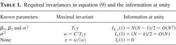
In (9) there are three nuisance parameters, β1, β2, and σ2. Theorem 1 deals with the information available for tests that are invariant with respect to a constant, trend, and length. The maximal invariant is derived via transformations of the data, as in

Within the context of (9) more restrictive models can be characterized by our knowing the values of the parameters. For example, if we knew all three values then y itself (or T1 y) would be the maximal invariant (in the trivial sense), and the information in T1 y is well known to be

On the other hand, for example, as in Müller and Elliott (2003), we could assume that the variance of ε in (1) is known (see their Condition 1). If length invariance is not required, only the first transformation in (10) is necessary, giving a maximal invariant

. Fisher information in w is readily found to be

Thus for three cases in (9) we can evaluate the available information at unity, as shown in Table 1. Thus what we are able to assume is known in the model has a significant quantitative effect on the rate at which information accrues at unity.
Required invariances in equation (9) and the information at unity

3.5. Characterization of Information over (Non)stationarity Regimes
Because the majority of distributional approximations for unit root tests are derived via local-to-unity asymptotics (e.g., Phillips, 1987), part (ii) of Theorem 1 also gives the properties of Fisher information in any asymptotic neighborhood of unity. Specifically, for model (3) we find that for 1 − ρ = O(cN), where cN → 0 as N → ∞, Iv(ρ) is O(N2). Asymptotic distributional approximations are most conveniently made in the regime in which cN = c/N, for constant c, as in the work of Elliott et al. (1996), who derive “optimal” tests for c = 0 against c > 0.
However, other neighborhoods are of interest, for example, if

, which corresponds with the limiting cases of both Chan and Wei (1987) and Phillips (1987). In this neighborhood, at least in the simplest autoregression, asymptotic normality of estimators may obtain, rather than the Weiner process driven asymptotics of the former case; see Phillips and Magdalinos (2007). Theorem 1 demonstrates that for any asymptotic neighborhood of unity the rate of increase in available information is O(N2). Information is zero only at the point ρ = 1.
From Theorem 1 we can asymptotically quantify the available information in the three regimes of interest. Letting the autoregressive parameter be ρ = 1 − O(cN), then as N → ∞ we can characterize the unit root regime as cN = 0, any local-to-unity regime as cN = o(1), and the stationary regime as cN = O(1). For the stationary case, consider the transformations in (10), so that we can write the density of y as

hence the information in y may be partitioned as

where

Because information is nonnegative we have Iv(ρ) ≤ Iy(ρ) = O(N) for |ρ| < 1.
To summarize, suppose that the autoregressive parameter is ρ = 1 − O(cN) ∈ (−1,1]; then in these regimes and as N → ∞,

3.6. Information and Power
The direct effect on power of information being zero can be explored via a simple example. Suppose that we have a sample of size N on xi ∼ iidN(μk,1), k ≥ 1 and known. In this case it is trivial to establish that Fisher information is zero at μ = 0 and that the maximum likelihood estimator (the global maximum of the likelihood) is

. The immediate implication is that uniform convergence is lost, in that

which in turn affects the rate of asymptotic power because all tests have to be a function of

, the sufficient statistic in this case.
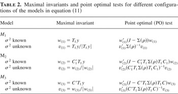
The consequences for the unit root model are not as obvious. However, part (iii) of Theorem 1 does provide an alternative link between power and information. As was seen in Section 3.4, there is an intimate relationship between what we are willing to assume as known in the model, and hence the required invariances, and information at unity. We can also, therefore, explore the impact that the invariance requirements have on the power envelope for the unit root. For model (9) we can characterize six different cases. For the purposes of experiment these can be represented by data (yt)1N generated by

where ut = ρut−1 + εt, εt ∼ iidN(0,σ2) and for each model σ2 will either be presumed known (σ2 = 1) or unknown. For each case both the maximal invariant and the point optimal (PO) test can easily be derived. If we also define a matrix C1, so that

then for each case the results shown in Table 2 pertain.
Maximal invariants and point optimal tests for different configurations of the models in equation (11)

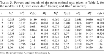
In each case the PO test rejects for observed outcomes smaller than some pre-specified constant, chosen so that the size is fixed at δ = 0.05. The power of all of these PO tests was simulated via experiments analogous to those giving the power envelopes in Elliott et al. (1996). Put ρ = 1 − c/N, fix the sample size at N = 500, and on the basis of 100,000 replications the critical values are calculated and then from those, the power under alternatives parameterized by c = 1,2,3,…,25.
The most restrictive case (M1, σ2 known) provides an absolute power upper bound, in that the Neyman–Pearson lemma applies in the strictest sense. All other cases can be compared to this benchmark. Of interest are the values of c at which the power envelope is 0.5, the point at which Elliott et al. (1996) define their nearly efficient test. For the most restrictive case this is approximately 6.5, whereas for the most general it is 13.5 (M3, σ2 unknown). Collectively the results are really self-explanatory. Of note though are two things. Near the null hypothesis the effect of requiring both trend and length invariance is dramatic, implying powers close to just 20% of benchmark. Additionally, the assumption that σ2 is known is not quite as benign as perhaps suggested in Müller and Elliott (2003). Although what is clear is that what is most crucial is the trend, because then the assumption about σ2 has the greatest effect, it is also clear that a consistent procedure for determining the necessity of a trend, such as in Bunzel and Vogelsang (2003), may have a significant bearing on our subsequent ability to correctly detect a unit root.
Contained in Table 3 are illustrations of the power bound of part (iii) of Theorem 1. In general the bound on the power of any invariant test for (2) in the context of the models Mi (with variance unknown) of (11) is

Notice that the bound explicitly tightens for M3 in that the first term vanishes as a result of Sv(3)(1) = 0, as indicated by part (iii) of Theorem 1. An alternative bound is obtained by applying

to (12). This gives a slightly weaker bound, depending only on information, but that applies in cases where the score is not identically zero.
Powers and bounds of the point optimal tests given in Table 2, for the models in (11) with cases A(σ2 known) and B(σ2 unknown)

These results are very important from a theoretical view, being the first explicit links between power and information. Because for nonergodic models the role of Fisher–Rao theory is at best ambiguous, this result retains a role for information. Practically its usefulness is less obvious. It is an existence result. Although numerically we can always find a particular ρ* such that the bound is as tight as our numerical accuracy permits, this has to be done pointwise. For a practical bound put ρ* = 1 − c*/N, and the bounds in (12) become

Moreover, because Iv(3)(1) = 0, then for sufficiently large N we must have Iv(3)(1 − c*/N) ≤ Iv(3)(1 − c/N) if c* ≤ c. Consequently, we can utilize the following locally uniform bound for M3:

In addition to the power envelopes Table 3 also contains the appropriate values for P3(c) and also, although local uniformity may not apply, for P1(c) and P2(c), for which the term E [|Sv(i)(1)|] was approximated via the simulations described previously. Numerically the importance of the vanishing of the score is highlighted, although because at each value of c it is possible to improve the bound arbitrarily, no further importance can be attached. Instead, if we seek to measure efficiency in terms of how tests are able to discriminate between the null and alternative given particular mean functions, a more practical measure would be to use an explicit measure of distance, such as that proposed in Marsh (2005).
4. CONCLUSIONS
This paper has proved that inclusion of a trend in the Sargan and Bhargava (1983) formulation implies zero available information at the unit root. The explicit bound on power by information implies that low power is an inevitable consequence of trend invariance. This precise relationship between the inclusion of a trend and information at the unit root and also the explicit bound on the power of invariant unit root tests add significantly to our understanding of this problem.
Specifically, the relationship between unit root and trend is captured algebraically by (6). That is, the consequence of requiring invariance to a trend produces this identity, which in turn implies that Fisher information is zero. This identity is essentially unchanged if we difference the data any number of times. Consequently, at the unit root, there is a complete equivalence between differencing and projecting orthogonally to a trend.
APPENDIX
Proof of Lemma 1. Part (i) follows immediately from the results of King (1980).
For part (ii), we have that the log-likelihood is

and hence the score is

and so information is obtained as

By definition, E [Sv(ρ)] = 0 immediately implies

so that the only other expectation to be calculated is

Noting that we can write v = w/|w|, where w is spherically symmetric with mean zero and Var[w] = A, then

where

and z = A−1/2w. Further, because rz is independent of

, we have

and hence

The expression for the information follows from squaring (A.1), utilizing the expectations given in (A.2) and (A.3), and rearranging. █
Proof of Theorem 1. For part (i), from Lemma 1, Fisher information in v at ρ = 1 is given by

where

and the derivative of the covariance matrix is

so that

where S = T1−1, is the lower-triangular partial summation matrix. Consider the derivative of the matrix Σρ = Σρ(IN),

which at the unit root evaluates to

From the identity

where τ = (1,2,3,…, N)′ and substituting L(1) = IN − T1 into (A.5), we obtain

which forms the fundamental relationship between the unit root covariance and the time trend.
Because Ω is Toeplitz and symmetric we can write

where Lk = (L(1))k, and put L0 + L0′ = I, so that

Furthermore, L(1)S = (S − IN) = SL(1), and hence

The last term in (A.7) is just −A1, and the quadratic forms in C′ can be rewritten, as in

where we have exploited (S − IN)Lk = Lk(S − IN). Thus using (A.6), we have

and finally because (T1τ)′C = 0 = C′(T1τ), as X includes a trend, then A1 = −A1, and substitution into (A.4) gives, as required, Iv(1) = 0.
For part (ii), we require an expansion of the matrices A−1 and A appearing in (5). To proceed consider the matrix defined by

Letting ρ = e−cN, so that 1 − ρ = O(cN) with cN → 0, and putting ck* ∈ (0,cN) for k = 1,2,…, N − 1, then each lower diagonal of Tc−1 = Tρ−1 has a mean value expansion, so that

where Lk is defined in the proof of part (i).
Application of the expansion given in (A.8) yields

where

with W1 = SL(1)SΩS*′, W2 = SL(1)S*ΩS*′, and W3 = S*L(1)S*ΩS*′. Using SL(1) = I − S and the fact that S* commutes with Lk, then similar to the steps taken toward the end of the proof of part (i) we can show that

Consequently, and because Q2 is symmetric, we have

that is, the leading terms of A2 and Q1 are proportional.
We require an expansion for A−1 and so notice that

implies that as N → ∞, cN → 0, AA1−1 → I, and hence for any

,

Now define an Nk such that for all N ≥ Nk,

Consequently, all asymptotic statements to follow are to be interpreted as N ≥ Nk, Nk → ∞, which implies cN → 0.
To proceed, we can write

where

and convergence of the summation is asymptotic, as cN → 0. The crucial quantity appearing in (5) may therefore be written as

Squaring (A.12) and taking the trace we have

and taking the trace of (A.12) and then squaring we obtain

Thus, for sufficiently large N, for 1 − ρ = O(cN) and from (A.13) and (A.14), we have

If we utilize the expansions given in (A.9) and the proportionality in (A.10), then the information has an asymptotic leading term of

From the inequalities

and noting that (A.11) implies that for N ≥ Nk the eigenvalues of cN A2 A1−1 are O(1), we have

which subsequently implies that

For part (iii), let

be the rejection region for any invariant test, having size δ, of H0 : ρ = 1 against H1 : |ρ| < 1. Let

be the power of that region and define the power gain (i.e., power minus size) as

Following Würtz (1997) the power gain satisfies the following bound:

where Δ(1,ρ) is called the displacement function and ∥.∥1 is the L1 norm.
By Taylor's theorem we may write

for some

, and we have written

Further, we can write

where

so that

Thus we have

and we can define ρ* according to

Then because E [(Sv(ρ))2] = E [−Hv(ρ)] we have

Now partition the unit sphere into two regions,

with

so that

because −Hv(ρ*) + |Hv(ρ*)| = 0 on s2(v). Consequently,

because both Hv(ρ*) and f (v;ρ*) are positive on s2(v). Thus we have

where Iv(ρ*) is Fisher information evaluated at ρ = ρ*.
Irrespective of the particular set of regressors, from (A.15) it follows that

When the set of regressors includes a linear trend we have

where A and A are defined earlier in this proof. Thus at ρ = 1,

because A1 = (dA)ρ=1 = −A1. Substituting (A.17) into (A.16) and putting cN = 1 − ρ and c* = 1 − ρ* gives the result. █