



1 Introduction
In a diurnal cycle, differential heating and cooling of the atmospheric boundary layer (ABL) by the ground leads to variable turbulent flow characteristics. During the neutrally stratified periods, turbulence is mainly generated by vertical shear, while during the unstably stratified periods, thermally-driven buoyancy plays an important role in the production of turbulence (Stull Reference Stull1988). As the ground surface heats up, the near-surface flow warms with it and buoyancy makes a positive contribution to the energy budget, thus enhancing vertical mixing and production of turbulence kinetic energy (TKE). Conversely, during periods of stable stratification, turbulence is mainly dissipated by buoyancy, resulting in a strong reduction in mixing (Garratt Reference Garratt1994; Mahrt Reference Mahrt1999; Abkar, Sharifi & Porté-Agel Reference Abkar, Sharifi and Porté-Agel2016). Consequently, performance of wind farms strongly depends on the atmospheric stratification, see Hansen et al. (Reference Hansen, Barthelmie, Jensen and Sommer2012), Wharton & Lundquist (Reference Wharton and Lundquist2012), Abkar et al. (Reference Abkar, Sharifi and Porté-Agel2016), Cortina, Cal & Calaf (Reference Cortina, Cal and Calaf2016) and StMartin et al. (Reference StMartin, Lundquist, Clifton, Poulos and Schreck2016). Therefore, understanding the interaction of wind farms with the time-changing thermal stratification in the atmosphere is critical for an efficient development of wind energy resources.
In reviewing the equations for momentum, mean kinetic energy and turbulence kinetic energy, the footprint of thermal stratification is expressed by a corresponding additional source/sink buoyancy term. It is this additional term that perturbs the canonical, neutrally stratified, wind turbine array boundary layer (WTABL) flow. A recent work of Cortina et al. (Reference Cortina, Cal and Calaf2016) developed a detailed mean kinetic energy (MKE) budget, using a control volume approach, to characterize the processes of MKE recovery under different thermal stratification. Results illustrated that under a convective (unstable) stratification the MKE energy depleted by the turbine is mainly recovered by an enhanced vertical flux of MKE. Contrarily, under stable stratification conditions, the MKE is mainly replenished through advection of MKE. These changes in the predominant mechanisms for recovery of MKE respond to a subjacent change in turbulence structure. In this regard, Chamorro & Porté-Agel (Reference Chamorro and Porté-Agel2010) found that in a stably stratified ABL flow there is a steepening of the power law describing the turbulence decay in the near-wake region. This means that under stably stratified flow regimes turbulence mixing decays much faster, inhibiting recovery through turbulent fluxes of MKE in the wake region of the turbines. Also, Zhang, Markfort & Porté-Agel (Reference Zhang, Markfort and Porté-Agel2013) found a velocity reduction of
 ${\sim}15\,\%$
at the wake centre under convective regimes in comparison to that encountered under neutrally stratified conditions, a result of the enhanced turbulent mixing and decrease in MKE. Using experimental data from the Nysted offshore wind farm, Barthelmie & Jensen (Reference Barthelmie and Jensen2010) found that under stable conditions the wind farm harvested power is reduced as a result of the persistent wake–turbine interactions. This was also found to be the case in the Horns Rev wind farm, where the decrease in turbulence intensity was shown to produce more intense wake deficits, leading to the decrease of the harvested power of the overall farm (Hansen et al.
Reference Hansen, Barthelmie, Jensen and Sommer2012). It is therefore evident that turbulence structure and intensity play major roles in the recovery process of MKE in the wake of wind turbines as well as on the overall power produced by a wind farm. However, at this point little is known regarding the changes in the ABL turbulence structure resulting from including wind turbines and considering thermal stratification (i.e. the thermal WTABL). To overcome this important knowledge gap, a proper orthogonal decomposition (POD) of the turbulent flow is employed.
POD is a mathematical technique based on the Hilbert–Schmidt theory that was first introduced in turbulence analysis as a means to identify coherent turbulent structures in fluid flows (Lumley Reference Lumley1967). This technique has been effectively applied over a vast range of turbulent flows, including the atmospheric flows and wind turbine wakes. For example, Shah & Bou-Zeid (Reference Shah and Bou-Zeid2014) applied the POD technique to thermally stratified ABL flows to study the existence of large-scale turbulent features, showing that the effect of buoyancy flux in the dominant POD modes is significant to the energy balance. Streamwise rolls were observed in the first POD modes of the unstable case, which were not apparent in the stable case. Further, under unstable stratification, the first modes illustrated sheet-like motions, i.e. motions located in regions of low rotation and not contributing to vortical structures. With regard to the turbulent flow in wind farms, VerHulst & Meneveau (Reference VerHulst and Meneveau2014) used POD to study the structure of turbulence in the canonical, neutral WTABL. Results illustrated the contribution of individual POD modes to the energy entrainment as a function of wind farm layout. Also, Andersen, Sørensen & Mikkelsen (Reference Andersen, Sørensen and Mikkelsen2013) used POD to analyse the LES data of a large wind farm, showing that the dynamics of the wake meandering have a strong dependence on the spacing between turbines. It was shown that the first 10 modes were enough to capture more than 51 % of the total turbulence kinetic energy, and that the following 400 modes captured less than 40 %. Bastine et al. (Reference Bastine, Witha, Wächter and Peinke2015) developed a POD analysis of LES data of a characteristic wind turbine wake. From the results, it was possible to identify spatial modes characteristic of the wake of the isolated wind turbine. In that study, a few modes were sufficient to capture the dynamics of the flow, with the first mode being solely related to the horizontal movement of large-scale turbulence. More recently, Hamilton, Tutkun & Cal (Reference Hamilton, Tutkun and Cal2015) used POD to identify the coherent structures in the wind turbine wake of aligned and staggered wind farm configurations, showing that the turbulent flux and production are reconstructed with only 1 % of the total orthogonal POD modes. In a following experimental work, Hamilton, Tutkun & Cal (Reference Hamilton, Tutkun and Cal2016) developed the double POD in the wind turbine wakes to identify the sub-model organization of the largest projection and coefficients of the correction modes. Using this approach, it was possible to represent the turbine wakes with only 0.015 % of the total degrees of freedom of the original flow field.
Although important progress has been made in understanding the turbulence structure either in a single wind turbine wake, or in large wind farms under neutral conditions, further could be known about the effects of turbulence under thermal stratification. This is the focus of the present work, namely to generate knowledge about the structure of turbulence in the thermal WTABL. For this purpose, and given the proven strength of the POD technique, the snapshot POD technique is used. Therefore, the structure of the paper is as follows: in § 2, the LES computational set-up and study cases are presented. In § 3, results are presented, illustrating the differences in the POD energy and the POD modes. Finally, conclusions are presented in § 4. In the appendix, the LES governing equations and the theoretical formulation for the proper orthogonal decomposition are described.
2 Study cases
To simulate the atmospheric flow throughout a diurnal cycle, an atmospheric LES code has been used to integrate the non-dimensional, filtered, incompressible Navier–Stokes equations, together with the continuity equation and an advection–diffusion equation for the potential temperature (see appendix A for further details). Within the LES, wind turbines are modelled using the actuator disk with rotation approach of Wu & Porté-agel (Reference Wu and Porté-agel2011) including the capacity of self-alignment with the incoming mean wind of Sharma et al. (Reference Sharma, Calaf, Lehning and Parlange2016). Turbines have a hub-height and rotor-diameter (
 $D$
) of 100 m, scan a distance
 $D/2$
upstream of the rotor disk to learn about the incoming wind vector, and realign with the mean flow every ten minutes (Cortina, Sharma & Calaf Reference Cortina, Sharma and Calaf2017a
). The LES study cases (see table 1) are forced with a time-constant and height-independent geostrophic wind, whose values are extracted from the CASES-99 field experiment between 22–24 October, 1999, and are equal to
 $(U_{G},V_{G})=(9,-3)~\text{ms}^{-1}$
. In parallel, a time-varying surface temperature is imposed (see figure 2). The time period used to force the diurnal cycle has been used in other wind farm studies (Fitch, Lundquist & Olson Reference Fitch, Lundquist and Olson2013; Cortina et al.
Reference Cortina, Cal and Calaf2016; Sharma, Parlange & Calaf Reference Sharma, Parlange and Calaf2016; Cortina & Calaf Reference Cortina and Calaf2017; Cortina, Sharma & Calaf Reference Cortina, Sharma and Calaf2017b
); and hence the same forcing is employed here.
Perspective view (a) and top view (b) of the LES domain for the wind farm scenario.

(a) Represents the spatially averaged and time-dependent imposed temperature at the surface of the domain
 $\langle T_{s}\rangle _{1,2}$
in Kelvin; (b) represents the normalized stability parameter,
 $z_{1}/\langle L\rangle _{1,2}$
, where
 $(z_{1}=\unicode[STIX]{x0394}z/2)$
is the height of the first grid point and
 $L$
is the Monin–Obukhov length, as a function of time. Note that
 $\langle \cdot \rangle _{1,2}$
indicates the spatial average operation, in the streamwise and spanwise direction.

The numerical domain used for this study is set to,
 $L_{x}=2\unicode[STIX]{x03C0}z_{i}$
in the streamwise direction,
 $L_{y}=\unicode[STIX]{x03C0}z_{i}$
in the spanwise direction and
 $L_{z}=3z_{i}$
in the vertical direction (see figure 1 for a sketch visualization of the numerical domain), where
 $z_{i}$
is the height of the boundary layer at the beginning of the diurnal cycle – located at 1000 m of height. To retain a high numerical resolution, the computational domain is discretized with a numerical grid of
 $256\times 128\times 384$
grid points, providing a uniform grid resolution of
 $\unicode[STIX]{x1D6E5}_{x}=\unicode[STIX]{x1D6E5}_{y}=24.5~\text{m}$
and
 $\unicode[STIX]{x1D6E5}_{z}=7.8~\text{m}$
. This resolution suffices to produce good results due to the weak stable stratification characteristic of the diurnal cycle employed in this work, and the outstanding performance of the Lagrangian scale-dependent model (Bou-Zeid, Meneveau & Parlange Reference Bou-Zeid, Meneveau and Parlange2005), as noted in earlier LES studies of stable stratification (Kumar et al.
Reference Kumar, Svensson, Holtslag, Meneveau and Parlange2010). The simulations are initialized with the vertical velocity and temperature profiles extracted from Kumar et al. (Reference Kumar, Svensson, Holtslag, Meneveau and Parlange2010), corresponding to a height-independent geostrophic wind, and a well-mixed temperature profile matching the initial surface temperature of 278.6 K, with an inversion layer spanning from
 $z_{i}$
to the top of the domain (the capping inversion strength is set equal to
 $0.008~\text{K}~\text{m}^{-1}$
). Figure 2(a) illustrates the time evolution of the surface temperature used to force the flow, and the corresponding near-surface stability parameter (
 $z_{1}/L$
) is represented in figure 2(b), where
 $z_{1}$
is the height of the first grid point, equal to
 $\unicode[STIX]{x1D6E5}_{z}/2$
.
Summary of the different LES numerical study cases for a large array of wind turbines, referenced as wind farm (WF) and one without turbines, referenced as boundary layer (BL) under different atmospheric stratification: unstable, neutral and stable (U, N and S, respectively).

To develop this study, a suite of four different four-hour study periods are selected during the evolution of the diurnal cycle, representative of two different characteristic ABL stratification regimes (unstable and stable). These are marked in figure 2 with the black (
 $p$
1 and
 $p$
3) and red (
 $p$
2 and
 $p$
4) shading. More precisely time periods
 $p$
1 and
 $p$
3 constitute the times between 01:45 and 05:45h local time (representing stable stratification), and
 $p$
2 and
 $p$
4 represent the time between 13:15 and 17:15 of local time (representing unstable periods). Because neutral stratification conditions are ephemeral during the evolution of this specific diurnal cycle, an independent LES study with a conventional neutrally stratified flow is also considered. In order to obtain the neutrally stratified flow, thermal equilibrium is imposed between the surface and the air temperature profiles (cf. Sharma et al. (Reference Sharma, Parlange and Calaf2016)). Also, a four-hour study period is selected for the neutral simulation. Furthermore, for each characteristic stratification regime two different cases are considered, one without turbines (referenced as BL) and one with a large array of wind turbines (referenced as WF), adding up to a total of six different study cases. Note that in an earlier study by Cortina et al. (Reference Cortina, Cal and Calaf2016), it was shown that while the flow is highly variable throughout the two consecutive diurnal cycles, 10-minute statistics remain fairly stationary during the selected four-hour study periods marked in black and red in figure 2. Hence, in this work, statistics are directly computed over these four-hour periods, providing a means to compare the corresponding turbulence statistics under different thermal stratification regimes. See table 1 for more details about the different study cases. Hereon, the unstable stratification is denoted by U-WF and U-BL for the large array of wind turbines and without wind turbines, respectively; the neutral case is denoted by N-WF and N-BL and the stable case by S-WF and S-BL. In the wind farm cases, turbines are arranged in six columns of eight rows each, such that the corresponding turbine spacing is of
 ${\sim}7D$
and
 ${\sim}5D$
in the streamwise and spanwise directions, respectively, with
 $D$
indicating the turbine rotor diameter, here fixed to 100 m. To develop the POD analysis, a set of 1440 snapshots, spaced by 10 s, is used covering the full domain in the horizontal directions and expanding vertically between the ground surface and
 $z\approx 3D$
. This number of snapshots is set to provide converged statistics.
(a–d) Vertical profiles of mean wind speed,
 $\langle \overline{U}\rangle _{1,2}$
normalized by the geostrophic wind velocity
 $U_{G}$
, the wind veer,
 $\langle \overline{\unicode[STIX]{x1D6FC}}\rangle _{1,2}$
in degrees [deg.], the vertical shear,
 $\langle \overline{\unicode[STIX]{x1D70F}}\rangle _{1,2}$
normalized by the square of the geostrophic wind
 $U_{G}^{2}$
and the sensible heat flux,
 $\langle \overline{u_{3}^{\prime }\unicode[STIX]{x1D703}^{\prime }}\rangle _{1,2}$
, normalized by the geostrophic wind and a reference potential temperature
 $(U_{G},\unicode[STIX]{x1D703}_{o})$
, for the different atmospheric stability regimes: S-WF (●), S-BL (○), U-WF (▪), U-BL (▫), N-WF (▴), N-BL (▵). The shaded area represents the location of the rotor of the wind turbine, from
 $z/D=0.5$
to
 $z/D=1.5$
. The vertical axis is normalized by the wind turbine rotor diameter
 $D=100~\text{m}$
.

In figure 3(a–d), the vertical profiles of mean wind speed, wind veer, shear stress and sensible heat flux are presented. The vertical profiles are obtained by computing average values of the variables in space (streamwise and spanwise directions) and in time during the study periods delineated in figure 2, as well as the two neutrally stratified cases. The WF velocity profiles are normalized by the geostrophic wind speed,
 $\langle U\rangle _{1,2}/U_{G}$
, and depict a velocity deficit in the range of the wind turbine rotor disk (the shaded area between
 $z=0.5D$
and
 $z=1.5D$
). Among the different stability conditions for the WF, the unstable and neutral profiles are very similar, while the stable case shows the largest velocity deficit. For the BL cases, the velocities at the wind turbine rotor area are larger, also illustrating a similar shape between the neural and unstable profiles. Results illustrate an average
 $32\,\%$
velocity deficit at hub height when comparing the WF and the BL cases, due to the presence of the wind turbines. Both stable cases (the WF and BL) show a characteristic nocturnal low-level jet (LLJ). However, while the maximum velocity of the LLJ is located at a height of
 $z=1.5D$
in the absence of a wind farm, once the wind farm is introduced, the LLJ is vertically shifted above the wind farm, to a height of
 $z=5D$
. Also note that the WF scenarios present sharper velocity gradients between the bottom and the rotor top tip. Regarding the wind veer, it is observed that this one considerably increases in the presence of a wind farm. This difference is observed along the full domain height, up to the top of the boundary layer
 $z=z_{i}$
, where the vertical profiles merge at a wind veer equal to zero degrees. For neutral and unstably stratified cases, the relative difference in wind veer between the WF cases and the BL cases is approximately
 $10^{\circ }$
. The stable regime presents larger variations in wind veer (
 $15^{\circ }$
) at hub height, with even larger differences near the surface. Note that in general, the vertical wind veer is more pronounced during the stable regime, with a difference of
 $26^{\circ }$
from bottom to top tip. Large gradients in wind veer within the rotor disk area induce significant loads on the turbine blades and can result in power losses due to an overall misalignment of the rotor disk.
In the normalized shear stress profiles,
 $\langle \unicode[STIX]{x1D70F}\rangle _{1,2}/U_{G}^{2}$
, the expected constant vertical reduction is observed in all cases without a wind farm (U-BL, N-BL and S-BL). When the wind farm is present, enhanced gradients across the wind turbines swept area are developed, leading to significantly larger values of shear stress at the top tip of the wind turbine rotor disk (
 $z=1.5D$
). The magnitudes of shear stress at top tip height are further pronounced in the unstable and neutral regimes as a result of increased mixing compared to the stable case, which shows reduced values of shear stress. The increase in the U-WF and N-WF is about 250 % and 150 % with respect to the S-WF. The largest change when comparing the shear stress between WF and BL cases occurs under unstable stratification, with a 167 % increase.
For the sensible heat flux,
 $\langle \overline{u_{3}^{\prime }\unicode[STIX]{x1D703}^{\prime }}\rangle _{1,2}$
, both the U-WF and U-BL cases show positive values near the surface, extending up to
 $z/D=5.5$
, where the heat flux becomes zero. Thereafter, the heat flux displays a small negative value arising from the effect of the capping inversion, where the higher potential temperature flow from the free atmosphere is entrained downward. During the stably stratified periods, profiles of heat flux present sharper differences between the S-BL and S-WF cases, especially near the surface and within the rotor disk region. While in the S-BL case the negative buoyancy decreases linearly with height until reaching the zero-flux limit at near
 $1.5D$
height, in the S-WF case the flux presents a differentiated behaviour, with a sharp gradient below the rotor disk, and a gentler slope above. In the S-WF case, the zero-flux limit is reached near the
 $5.5D$
height, illustrating the induced growth of the boundary layer as a result of the enhanced mixing by the presence of the turbines. These results agree well with previous studies of the thermally stratified WTABL flows (Calaf, Parlange & Meneveau Reference Calaf, Parlange and Meneveau2011; Wu & Porté-agel Reference Wu and Porté-agel2011; Abkar & Porté-Agel Reference Abkar and Porté-Agel2014; Sharma et al.
Reference Sharma, Parlange and Calaf2016).
3 POD analysis
For the development of this work, snapshot POD is employed. The full theoretical development is not included in the main body of the text but rather provided in appendix B. Thus equations referenced in this section may be found in the appendix.
3.1 POD energy, a quantitative approach
The spatial integration of the TKE in a finite domain can be determined through the trace of the eigenvalue matrix (see (B 7)). The cumulative turbulence kinetic energy,
 $A_{n}$
, computed from (B 11) is presented in figure 4(a) for the WF and BL cases under unstable, stable and neutral stratification. To illustrate the energy associated with low-rank modes, the main figure only shows the TKE of the first 200 modes; the inset figure shows the TKE for the full modal basis. In the U-WF case, a rapid growth of the cumulative energy is observed. The initial modes contain most of the energy of the flow field and only a small number of modes is required to capture the majority of TKE (Andersen et al.
Reference Andersen, Sørensen and Mikkelsen2013; VerHulst & Meneveau Reference VerHulst and Meneveau2014; Hamilton et al.
Reference Hamilton, Tutkun and Cal2015). In the other stratification conditions, a greater number of modes is required to represent the full energy of the flow, indicating that intermediate and higher-order modes are more important than in the unstable cases. With increasing atmospheric stability, the growth of the cumulative energy,
 $A_{n}$
, slows down as a result of the reduction in high energy, large-scale mixing. The N-WF case shows moderate convergence lagging behind the U-WF case and passes the S-WF case after the first 35 modes. Interestingly, the neutrally stratified WF (N-WF) case lies between the convergence profiles of the U-WF and S-WF cases, in the range of modes 50–150. From this figure, it is also of relevance the rapid growth in cumulative energy with only the first few modes in the S-BL case. This is indicative of the fact that under stable conditions, turbulence is dominated by few highly organized structures and complemented by a large set of substantially less energetic turbulent modes. In the S-WF case however, this growth is cut by a factor of two in the presence of turbines, thus representative of the most energetic structures. This is symptomatic of the energy homogenization effect induced by the turbines.
Normalized turbulence kinetic energy based on the POD eigenvalues. The cumulative energy
 $A_{n}$
is illustrated in (a) and the energy per mode
 $B_{n}$
, is represented in (b). The dashed lines represent cases without wind farm (BL) and solid lines represent cases with a wind farm (WF), for the different stratification conditions, following this order: unstable-WF (▪), unstable-BL (▫), stable-WF (●), stable-BL (○), neutral-WF (▴), neutral-BL (▵). (c) Illustrates the efficiency coefficient (
 $\unicode[STIX]{x1D702}_{n}$
).

Alternatively, figure 4(b) illustrates the normalized TKE,
 $B_{n}$
, associated with each POD mode (see (B 12)). For the WF cases, the first mode varies by less than 4.5 %, although mode 1 represents a different percentage of TKE for each thermal stratification case. In contrast, when no turbines are present the TKE contribution of the first modes differ by 47 % between the S-BL and N-BL cases. By further evaluating the corresponding contribution of TKE from the different POD modes, each pair of cases (WF, BL), approximately converges beyond POD mode ten, especially visible in the unstably and neutrally stratified cases. It is therefore of relevance to note that the wind turbines drastically affect the structure and energy distribution through the first 10 POD modes, which represent 26 % and 14 % of the TKE in the U-BL and N-BL cases, respectively. For the stable scenario the TKE is strongly attenuated after the third POD mode, beyond which the corresponding contribution of each mode is more uniform. Contrarily, for the WF cases even, the higher POD modes provide a significant contribution to the TKE of the system up to mode six. As a result of the enhanced mixing produced by the turbines, the otherwise dominant turbulent structures present in the BL-flow are altered, with a noticeable decrease in energy for the unstable and stable cases, and an increase for the neutral case.
To further quantify the changes induced by the presence of large arrays of wind turbines in an otherwise unperturbed BL flow, and also as a function of thermal stratification two additional comparison variables are introduced:
(a) POD basis efficiency coefficient: this coefficient represents the capacity of a given POD basis to perform similar to the POD basis representative of a convective boundary layer, both in the presence or absence of turbines. This coefficient solely provides a comparison as a function of thermal stratification and is defined as:
 $$\begin{eqnarray}\unicode[STIX]{x1D702}_{n}=\frac{A_{n}(\text{unstable})-A_{n}(\text{case})}{A_{n}(\text{unstable})}.\end{eqnarray}$$
Positive or negative values of
 $\unicode[STIX]{x1D702}_{n}$
respectively represent a decrease or increase in efficiency of a given POD basis to represent the TKE compared to that under unstable stratification, see figure 4(c). Characteristically, when the efficiency coefficient (
 $\unicode[STIX]{x1D702}_{n}$
) is null, there is no difference in TKE distribution between the study case and the thermally unstable case. Results illustrated in figure 4(c) exhibit a distinctive behaviour for the S-BL case, where the first few modes exhibit a negative
 $\unicode[STIX]{x1D702}_{n}$
, exceeding the TKE of the U-BL. After mode 100, the distribution becomes positive and converges to zero after mode 1200. The N-BL always remains positive as reflected in the profile. The first mode carries a significant variation with respect to the U-BL, which thereafter decreases with increasing number of POD mode until converging to zero. The influence of the wind farm is evident especially in the stable case, where the efficiency parameter is positive throughout. This means that the cumulative TKE in the U-WF exceeds that of the S-WF for the first 1200 modes. The same behaviour is shown in the N-WF.
Bar representation of the wind farm disruption coefficient (
 $\unicode[STIX]{x1D6FF}B_{n}$
) for the different study cases (stable,


(b) Wind Farm disruption coefficient: to specifically quantify the effect of installing turbines on the TKE of the ABL, a parameter is defined by subtracting the corresponding TKE percentage representation between the WF and BL cases for each stratification case. The WF disruption coefficient therefore compares the structure of the turbulent flow for each thermal stratification with and without presence of a wind farm. This is represented in figure 5 and defined as,
 $$\begin{eqnarray}\unicode[STIX]{x1D6FF}B_{n}=\frac{B_{n}(\text{WF})-B_{n}(\text{BL})}{B_{n}(\text{WF})}.\end{eqnarray}$$
As expected from the normalized POD eigenvalues, the largest differences between the WF and BL cases are observed in the first POD mode. In this case negative values indicate that the otherwise undisturbed ABL case carries more TKE, and positive values of
 $\unicode[STIX]{x1D6FF}B_{n}$
indicate that the POD modes carry more TKE in the presence of a wind farm. For example, in mode 1 of the stable and unstable stratification cases, the BL alone communicates 850 % and 75 % more energy than in the WF cases, respectively. It is also of interest to note the consistent increase in TKE percentage through the first 20 POD modes of the S-WF and N-WF cases. Thereafter, there is a progressive decrease in
 $\unicode[STIX]{x1D6FF}B_{n}$
with increasing mode number. Contrarily, for the unstable case, in the presence of turbines, the corresponding TKE partition in each mode seems to be slightly reduced (on average about 12 % up until mode 20) in comparison to the case when there are no turbines. As a result, large wind farms have a relevant impact on the internal structure of the ABL, modifying the most energetic turbulent scales and redistributing the TKE more uniformly throughout the subsequent range of scales.
3.2 POD modes, a qualitative representation
Given that the overall TKE is accounted for in the modal decomposition (see § 3.1), observing particular modes, especially those with high energy content (lower index), is of interest to understand the dominant structure of the flow. Figures 6 and 7 present selected POD modes representing the structural differences between test cases. Each panel consists of a three-dimensional representation of the POD modes, with the
 $x$
-axis indicating the main streamwise direction, the
 $y$
-axis referring to the spanwise direction and the
 $z$
-axis indicating height. For better representation,
 $x$
and
 $y$
coordinates are normalized by
 $R=z_{i}/4$
, and the height (
 $z$
) is normalized by the rotor diameter (
 $D$
). Two horizontal (
 $x$
–
 $y$
) planes are represented, one at the surface and one of reduced size at hub height marked with white lines. Two vertical planes (
 $x$
–
 $z$
and
 $y$
–
 $z$
) are also represented at the edges of the numerical domain. Finally, an additional vertical plane aligned with the mean wind direction at hub height demonstrates contours of each mode and highlights the wakes. All selected POD modes are plotted with the same format.
First POD mode (a–f) and second POD mode (g–l) for the WF cases (a–c, g–i) and the BL cases (d–f, j–l) and for the different thermal stratification conditions, unstable (a,d,g,j), neutral (b,e,h,k) and stable (c,f,i,l). The POD modes represent the eigenvectors of the covariance matrix, and hence are presented without a colour bar because they do not carry physical meaning until they are recombined with the respective coefficients, which carry the physical units. As a result, there is no actual associated ‘magnitude’.

Third POD mode (a–f) and fourth POD mode (g–l), for the WF cases (a–c,g–i) and the BL cases (d–f,j–l) and for the different thermal stratification conditions, unstable (a,d,g,j), neutral (b,e,h,k) and stable (c,f,i,l).

The first POD mode (figure 6 a–f) of the S-WF case shows large features at the ground exhibiting Fourier-like behaviour and causing minimal mixing as a result of a decreased shear stress (see figure 3). The rotation of the turbines is captured through this mode in the diagonal plane. For the U-WF case, the first POD mode has a considerably larger vertical effect in comparison to the stably stratified case, which correlates with the enhanced vertical mixing observed in the vertical profiles of figure 3. Also, it can be seen in the U-WF case an imprint of the shearing due to the rotor, which is asymmetric due to the rotation of the turbine blades. A relatively large feature is observed in the diagonal plane. The N-WF case exhibits similar features to the U-WF case, although there is more coherence in the contours due to the decreased mixing. In the BL cases, the first mode of the stable stratification condition (S-BL) displays homogeneity both, in the horizontal and vertical directions. The U-BL case is less homogeneous and large-scale structures covering the entire domain are present. The neutral case (N-BL) manifests more roll-type structures that are advected with the flow (Shah & Bou-Zeid Reference Shah and Bou-Zeid2014; VerHulst & Meneveau Reference VerHulst and Meneveau2014), similar to those present in the N-WF case.
Although the second mode of the S-WF only carries approximately 70 % of the energy of the first mode (refer to figure 4), the structure of this mode is still remarkably coherent. The structure described by the basis of POD modes is related to the turbulent events in the flow, such as rolling structures, which may cover the full domain or be most visible near the surface. In this mode, wind turbine wakes are visible. Comparing the stratification regimes, the energy content in the U-WF case is twice as high as that of the N-WF case. The induced mixing is once again noted, with clear similarities between the structure of the mode near the ground and at hub height. Additionally, the (
 $x$
–
 $z$
) plane exhibits the interaction between the rotor and the flow above the canopy. In the BL case, the second mode of the stably stratified case (S-BL) displays small structures relatively near the surface, below where the hub would be located. This is different from mode one of the S-BL case, where relatively sizable features reside below hub height. The rolling structures shown in the S-WF case are absent in the S-BL case, indicating that installing a wind farm in the ABL not only increases mixing between flow layers, but also draws large structures down via entrainment processes. In contrast, the U-BL and N-BL cases while still exhibit rolling structures in the domain, their size is smaller when compared to the respective WF cases. This implies that turbine-induced mixing also generates a larger range of coherency in the turbulent field.
The third mode of the stable case (S-WF) shows approximately the same structure as the second mode, but shifted horizontally, which is a feature of POD (i.e. note that for any periodic dynamics, POD ascribes two POD modes with analogous energy and spectral contribution, but they are orthogonal being elements of the POD basis). The corresponding energy content of these modes is therefore similar. However, the third POD mode of the U-WF case holds half of the energy of the first two modes, which translates into smaller flow features. Furthermore, the near-surface region reflects the presence of the structures shown at hub height, indicating that wind turbines mostly dominate this mode. In the N-WF case, the flow structure near the surface is similar to that found in the U-WF case, whereas at the hub height the wake of the turbines is no longer evident. When no turbines are present, the structure of the S-BL case is composed of small features for
 $z/D<1.5$
. In the unstable and neutral cases (U-BL and N-BL), the structure of the third mode is similar to the structure of the second mode, including a horizontal shift in the
 $x$
-direction.
The fourth mode of the S-WF case shows streaks at the surface and deviates towards the streamwise direction, as shown in figure 7. The hub height continues to display the wakes of the turbines, also clear in the (
 $y$
–
 $z$
) plane, with the corresponding rotation of the rotor. Wake features disappear in the U-WF and N-WF cases, although at the surface features reflecting the wakes are present, emphasizing the impact of the wind farm on the structure of the flow. For the BL cases (unstable, stable and neutral), all display that the structure of the fourth mode is extremely similar to the structure of the third mode. Furthermore, the structure of the U-BL and N-BL cases are qualitatively similar to the fourth mode in the respective WF cases.
Three-dimensional representation of the POD modes for the WF cases.

For additional visualization, three-dimensional structures of the POD modes are presented in figure 8. From left to right, top to bottom are the U-WF, N-WF, S-WF and U-BL, first, second, third and hundredth POD modes. The format of this figure follows the same format of figures 6 and 7. The grey and orange colours present the negative and positive values of the modes, respectively. For the S-WF, long cylindrical structures covering the spanwise domain are observed in the first mode. The mixing between the wakes and the ABL structures is found in the U-WF and N-WF cases, where structures cover the full domain and the wakes are embedded inside the structures of the ABL. The S-WF case displays well-organized structures rotated as a result of the Coriolis force. This is specially clear in modes 2 and mode 4 illustrated in figure 8. The first and second modes of U-WF and N-WF display very large structures that cover the length of the physical domain and align perfectly with the streamwise direction. The wake structures are embedded inside these large structures. This result illustrates the fact that under unstable stratification, the influence of the Coriolis force on the large turbulence structures is diminished, while its effect remains relevant on the moderate and small turbulence structures. The dissipation of energy is observed with higher index of POD modes, where the structures become minuscule compared with those of low index, see for example mode 100. The neutral case displays moderately sized structures in mode 100, in contrast to the stable and unstable cases, which confirms intermediate and high index modes are more important in the N-WF case than in the S-WF or U-WF cases as shown in figure 4.
Three-dimensional representation of the POD modes for the BL case.

Without the presence of a wind farm, the neutrally stratified case (N-BL) shows the largest structures in the first four modes. These cover the full domain as shown in figure 9. These structures are not perfectly aligned with the streamwise direction, but deviate towards the diagonal of the domain as a result of the Coriolis force. The neutral case in figure 5 shows that the turbulent energy of the N-WF is larger than the energy of the N-BL case, confirming two points: first, the Coriolis force is an
 $O(1)$
term in the domain; and second, the transport of mean kinetic energy due to turbulence in the wind farm increases vertical entrainment. The U-BL case also shows large structures extending over the full domain, but in this case aligned in the streamwise direction.
4 Conclusions
LES is used to investigate the flow field in large wind farms embedded within an atmospheric boundary layer. Three different regimes of thermal stratification, stable, unstable and neutral have been considered to reproduce the characteristic flow conditions encountered in realistic atmospheric boundary layer flows. The turbulence structure of the flow under the presence or absence of wind farms has been characterized using the POD.
In the U-WF case results show a rapid convergence of cumulative energy, compared to the stable and neutral cases. Specifically, to capture 50 % of the total TKE requires 200 % and 80 % more modes for the stable and neutral cases in comparison to the unstable case, respectively. The modal bases of each case outlined by the POD display differing efficiency in terms of their account of TKE as a function of increasing number of cumulative modes. In the absence of turbines, turbulence in the S-BL case displays the fastest convergence of cumulative energy up to mode 100, thereafter lagging behind the U-BL case. By introducing the wind farm disruption coefficient, it is observed that large wind farms have a relevant impact on the internal structure of the ABL by modifying the most energetic turbulent scales, and redistributing TKE more uniformly throughout the subsequent range of scales. In this regard, it was further observed through the normalized TKE coefficient,
 $B_{n}$
, that WTs most drastically affect the structure and energy distribution of the flow through the first 10 POD modes, especially in neutral and convective conditions.
POD modes represent the optimal base structure of the flow in terms of the energy that they describe (VerHulst & Meneveau Reference VerHulst and Meneveau2014; Bastine et al. Reference Bastine, Witha, Wächter and Peinke2015; Hamilton et al. Reference Hamilton, Tutkun and Cal2015, Reference Hamilton, Tutkun and Cal2016; Hamilton, Tutkun & Cal Reference Hamilton, Tutkun and Cal2017). In this regard, the particular structure of the modes varies significantly with thermal stratification and the shear stress at different locations in the domain. In unstable and neutral conditions, thermal stratification damps much of the perturbation introduced by the turbines’ wakes, and hence not much difference is observed between cases with regard to the modal structure. Comparing the dominant POD modes, it can be concluded that during unstable and neutral conditions turbines minimally perturb the structure of the POD modes, while during stable conditions the structure of the turbulence field is strongly disrupted by the turbines. Additionally, in the S-WF case, Coriolis effects are relevant, affecting the overall structure of the ABL. At the surface, the flow presents a strong wave-like structure, which results of the continuous interaction of successive wind turbine wakes. On one side, the wake structure emanating from each turbine is visible, and on the other side, the effect of this wake propagates to the surface inducing the wave-type pattern. For the U-WF and N-WF cases, very large structures dominate, and do not include dominant features related to the turbine wakes.
The current study provides a new perspective on how wind turbines perturb the atmospheric flow under different thermal stratification conditions. The observations found in the current study will benefit the optimization and control of new generation wind farms under different thermal stratification conditions.
Acknowledgements
This work was in part funded by the National Science Foundation (CBET-1034581 and IGERT-0966376). Calaf acknowledges the Mechanical Engineering Department at University of Utah for start-up funds. The authors would like to recognize the computational support provided by the Center for High Performance Computing (CHPC) at University of Utah.
Appendix A. LES governing equations
The rotational form of the non-dimensional filtered, incompressible Navier–Stokes equations, along with the continuity equation and an advection–diffusion equation, have been used to simulate the thermally stratified atmospheric flow of a realistic atmospheric diurnal cycle,
 $$\begin{eqnarray}\displaystyle & & \displaystyle \frac{\unicode[STIX]{x2202}\tilde{u} _{i}}{\unicode[STIX]{x2202}t}+\tilde{u} _{j}\left(\frac{\unicode[STIX]{x2202}\tilde{u} _{i}}{\unicode[STIX]{x2202}x_{j}}-\frac{\unicode[STIX]{x2202}\tilde{u} _{j}}{\unicode[STIX]{x2202}x_{i}}\right)\nonumber\\ \displaystyle & & \displaystyle \quad =-\,\frac{1}{\unicode[STIX]{x1D70C}}\frac{\unicode[STIX]{x2202}p^{\ast }}{\unicode[STIX]{x2202}x_{i}}-\frac{\unicode[STIX]{x2202}\tilde{\unicode[STIX]{x1D70F}}_{ij}}{\unicode[STIX]{x2202}x_{j}}+g\left(\frac{\tilde{\unicode[STIX]{x1D703}}-\langle \tilde{\unicode[STIX]{x1D703}}\rangle }{\unicode[STIX]{x1D703}_{0}}\right)\unicode[STIX]{x1D6FF}_{i3}+f(\tilde{u} _{2}-U_{G_{2}})\unicode[STIX]{x1D6FF}_{i1}-f(\tilde{u} _{1}-U_{G_{1}})\unicode[STIX]{x1D6FF}_{i2}+f_{i},\hspace{24.0pt}\end{eqnarray}$$
 $$\begin{eqnarray}\displaystyle & \displaystyle \frac{\unicode[STIX]{x2202}\tilde{u} _{i}}{\unicode[STIX]{x2202}x_{i}}=0, & \displaystyle\end{eqnarray}$$
 $$\begin{eqnarray}\displaystyle & \displaystyle \frac{\unicode[STIX]{x2202}\tilde{\unicode[STIX]{x1D703}}}{\unicode[STIX]{x2202}t}+\tilde{u} _{j}\frac{\unicode[STIX]{x2202}\tilde{\unicode[STIX]{x1D703}}}{\unicode[STIX]{x2202}x_{j}}=-\frac{\unicode[STIX]{x2202}\unicode[STIX]{x03C0}_{j}}{\unicode[STIX]{x2202}x_{j}}. & \displaystyle\end{eqnarray}$$
Above,
 $\tilde{u} _{i}$
represents the LES filtered velocity, with the index notation used to specify rectangular Cartesian coordinates. The filtered potential temperature is represented by
 $\tilde{\unicode[STIX]{x1D703}}$
, the resolved dynamic pressure is represented by
 $p^{\ast }$
and
 $f$
is the Coriolis parameter. In addition, the tilde (
 $\tilde{\text{}}$
) represents the LES filtering operation at the grid size
 $\unicode[STIX]{x1D6E5}$
. The flow is forced via a height-independent geostrophic wind of
 $U_{G_{1}}=9~\text{ms}^{-1}$
in the streamwise direction and
 $U_{G_{2}}=-3~\text{ms}^{-1}$
in the spanwise direction. The influence of thermal stratification is included in the momentum equation by means of a buoyancy term resultant of considering the Boussinesq approximation (Stull Reference Stull1988). The filtered shear stress is represented by
 $\unicode[STIX]{x1D70F}_{ij}$
and its deviatoric part is modelled using the sub-grid Lagrangian scale-dependent model of Bou-Zeid et al. (Reference Bou-Zeid, Meneveau and Parlange2005). For the potential temperature, the sub-grid sensible heat flux
 $\unicode[STIX]{x03C0}_{j}$
from (A 3) is modelled using the Lagrangian scale-dependent model for scalars of Calaf et al. (Reference Calaf, Parlange and Meneveau2011). The modified kinematic pressure term (
 $p^{\ast }$
) includes the filtered pressure and the trace of the sub-grid scale (SGS) tensor
 $(\tilde{p}/\unicode[STIX]{x1D70C}+\tilde{\unicode[STIX]{x1D70F}}_{kk}/3+(\tilde{u} _{j}\tilde{u} _{j})/2)$
. The forcing exercised by the wind turbines on the flow is represented by a body force,
 $f_{i}$
. The actuator disk model with rotation and yaw alignment of Sharma et al. (Reference Sharma, Calaf, Lehning and Parlange2016) is used to represent the forces exerted by the wind turbines on the flow, here represented through
 $f_{i}$
. Therefore, the wind turbines timely readjust to the incoming wind every 10 min (Cortina et al.
Reference Cortina, Cal and Calaf2016, Reference Cortina, Sharma and Calaf2017b
; Cortina & Calaf Reference Cortina and Calaf2017) by measuring the incoming wind vector at a distance
 $D/2$
upstream of the rotor disk. In LES of atmospheric flows, viscous effects are neglected because the Reynolds number is very large. The differential equations are discretized using a pseudo-spectral discretization with a vertically staggered grid, where second-order finite differences are used to integrate in the vertical direction, similar to Moeng (Reference Moeng1984) and Albertson & Parlange (Reference Albertson and Parlange1999). Because of the use of spectral methods in the horizontal direction, the lateral boundary conditions are periodic, and thus results are in practical sense equivalent to a horizontally infinite domain. The equations are dealiased using the
 $3/2$
-rule (Canuto, Hussainii & Quarteroni Reference Canuto, Hussainii and Quarteroni1988), where the horizontal grid is expanded by a factor
 $3/2$
and padded with zeros for the product of the nonlinear terms. After the multiplication the resulting term is truncated back to the original grid size at each time iteration. The equations are time integrated using a second-order Adam–Bashforth scheme. The numerical algorithm is fully parallelized using the message-passing interface (MPI), where the pipeline Thomas algorithm (Povitsky & Morris Reference Povitsky and Morris2000) is used to parallelize the pressure solver. At the top of the domain a zero-flux boundary condition is imposed for momentum and temperature. At the surface the no-slip condition is applied for the vertical velocity, and because of the staggered grid, an equivalent shear stress is imposed at the first grid point for the horizontal momentum components and temperature. The shear stress at the surface is parameterized using the traditional log law including the effects of stratification (Monin & Obukhov Reference Monin and Obukhov1954; Parlange & Brustaert Reference Parlange and Brustaert1993; Bou-Zeid et al.
Reference Bou-Zeid, Meneveau and Parlange2005),
 $$\begin{eqnarray}\unicode[STIX]{x1D70F}_{i,3}(x,y,z_{1})=-\left[\frac{\unicode[STIX]{x1D705}\sqrt{(\hat{\tilde{u} }_{1}^{2}+\hat{\tilde{u} }_{2}^{2})}}{\ln (z_{1}/z_{0})+\unicode[STIX]{x1D713}_{m}(z_{1}/L)}\right]^{2}n_{i}.\end{eqnarray}$$
Note that
 $\unicode[STIX]{x1D705}$
is the von Kármán constant, which has been taken equal to 0.4, and
 $z_{1}$
is the height of the first staggered grid point, where the horizontal velocity components are computed (
 $z_{1}=\unicode[STIX]{x1D6E5}_{z}/2$
) and the shear stress is applied. Additionally,
 $z_{0}$
represents the ground surface roughness, which in this study is imposed as homogeneous and with a value of
 $z_{0}=3\times 10^{-5}z_{i}$
, where
 $z_{i}=1000$
m is the initial boundary layer height, which will be used as a normalization length scale. Further,
 $n_{i}$
is a unitary directional vector,
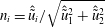 $n_{i}=\hat{\tilde{u} }_{i}/\sqrt{\hat{\tilde{u} }_{1}^{2}+\hat{\tilde{u} }_{2}^{2}}$
, where
 $i$
indicates any of the horizontal plane-parallel directions (
 $i=1,2$
). In addition to the shear stress at the surface, the vertical derivatives of the horizontal velocities are also parametrized at the first grid point
 $z_{1}$
(Brutsaert & Parlange Reference Brutsaert and Parlange1992),
 $$\begin{eqnarray}\unicode[STIX]{x2202}_{3}\tilde{u} _{i}(x,y,z_{1})=\left(\frac{\sqrt{\unicode[STIX]{x1D70F}}}{\unicode[STIX]{x1D705}z}\right)n_{i},\end{eqnarray}$$
with
 $\unicode[STIX]{x1D70F}=\sqrt{\unicode[STIX]{x1D70F}_{1,3}^{2}+\unicode[STIX]{x1D70F}_{2,3}^{2}}$
. To integrate equation (A 3) for the potential temperature, a time-varying surface temperature is imposed, from which the surface sensible heat flux is computed using Monin–Obukhov’s similarity theory and imposed at the first staggered grid point,
 $$\begin{eqnarray}H_{s}(x,y,z_{1})=\frac{\unicode[STIX]{x1D705}^{2}[\unicode[STIX]{x1D703}_{s}-\tilde{\unicode[STIX]{x1D703}}(x,y,z_{1})]\left(\sqrt{\hat{\tilde{u} }_{1}^{2}+\hat{\tilde{u} }_{2}^{2}}\right)}{\displaystyle \left[\ln \left(\frac{z_{1}}{z_{0}}\right)+\unicode[STIX]{x1D713}_{m}(z/L)\right]\left[\ln \left(\frac{z_{1}}{z_{0,h}}\right)+\unicode[STIX]{x1D713}_{h}(z/L)\right]}.\end{eqnarray}$$
In this case,
 $z_{0,h}$
represents the scalar surface roughness, which following Brutsaert, Parlange & Gash (Reference Brutsaert, Parlange and Gash1989) has been taken to be one tenth of the momentum surface roughness (
 $z_{0,h}=z_{0}/10$
). The stability correction functions
 $(\unicode[STIX]{x1D713}(z/L))$
implemented are those from Brutsaert (Reference Brutsaert2005). In this work it is well understood that the stability correction functions were initially developed from experimental studies on statistically homogeneous surfaces and that the wind turbines might have an effect on the precise parametrization of the stability correction functions. However, lack of new experimental data on this precise matter does not allow for a better numerical approach at the present time.
Appendix B. Snapshot proper orthogonal decomposition
The POD technique, also known as Karhunen–Loéve expansion or singular value decomposition, consists on a description of the turbulent flow field using a set of energy optimal deterministic basis functions, such that
 $$\begin{eqnarray}\boldsymbol{u}(\boldsymbol{x},t)=\mathop{\sum }_{j=1}^{N}a_{j}(t)\unicode[STIX]{x1D719}_{j}(\boldsymbol{x}).\end{eqnarray}$$
In this representation (B 1), the basis functions (
 $\unicode[STIX]{x1D719}_{j}(\boldsymbol{x})$
) are the eigenfunctions of the covariance tensor of the analysed process, and represent the typical realizations of the analysed process in a statistical sense. The mode coefficients,
 $a_{j}(t)$
, are the so-called principle components, which are a set of independent coefficients that carry the time dependency and can be obtained by back projecting the POD modes onto the stochastic velocity field,
 $$\begin{eqnarray}a_{j}(t)=\int _{\unicode[STIX]{x1D6FA}}\boldsymbol{u}(\boldsymbol{x},t)\unicode[STIX]{x1D719}_{j}(\boldsymbol{x})\,\text{d}\boldsymbol{x}.\end{eqnarray}$$
To determine the set of optimal base functions that conform the kernel of the POD (also called the covariance matrix), the fluctuating velocity field (
 $\boldsymbol{u}(\boldsymbol{x},t)$
) is computed from a set of flow snapshots that are traditionally organized in matrix form,
 $$\begin{eqnarray}\boldsymbol{u}(\boldsymbol{x},t)=\left(\begin{array}{@{}ccccc@{}}u_{1}^{1} & u_{1}^{2} & u_{1}^{3} & \cdots \, & u_{1}^{N}\\ \vdots & \vdots & \vdots & \vdots & \vdots \\ u_{M}^{1} & u_{M}^{2} & u_{M}^{3} & \cdots \, & u_{M}^{N}\\ v_{1}^{1} & v_{1}^{2} & v_{1}^{3} & \cdots \, & v_{1}^{N}\\ \vdots & \vdots & \vdots & \vdots & \vdots \\ v_{M}^{1} & v_{M}^{2} & v_{M}^{3} & \cdots \, & v_{M}^{N}\\ w_{1}^{1} & w_{1}^{2} & w_{1}^{3} & \cdots \, & w_{1}^{N}\\ \vdots & \vdots & \vdots & \vdots & \vdots \\ w_{M}^{1} & w_{M}^{2} & w_{M}^{3} & \cdots \, & w_{M}^{N}\end{array}\right),\end{eqnarray}$$
where
 $u$
,
 $v$
and
 $w$
, are the velocity fluctuations in the respectively streamwise, spanwise and wall-normal directions. Note that for the sake of clarity the apostrophe denoting the fluctuation has been omitted. Further, the superscript
 $N$
represents the number of snapshots for which the fluctuating velocity fields are available and subscript
 $M$
represents the number of spatial grid points conforming each snapshot, respectively. The kernel tensor or two-point correlation tensor is determined through the product of (B 3) with itself, such that
 $$\begin{eqnarray}R(\boldsymbol{x},\boldsymbol{x}^{\prime })=\frac{1}{N}\mathop{\sum }_{j=1}^{N}u^{T}(\boldsymbol{x},t)\otimes u(\boldsymbol{x}^{\prime },t),\end{eqnarray}$$
where
 $R(\boldsymbol{x},\boldsymbol{x}^{\prime })$
denotes the spatial correlation between two points
 $\boldsymbol{x}$
and
 $\boldsymbol{x}^{\prime }$
and the superscript
 $T$
denotes the transpose operation. This kernel provides the optimal projection onto the flow field, which is acquired by the calculus of variations and following the Fredholm integral equation,
 $$\begin{eqnarray}\int _{\unicode[STIX]{x1D6FA}}R(\boldsymbol{x},\boldsymbol{x}^{\prime })\unicode[STIX]{x1D719}(\boldsymbol{x}^{\prime })\,\text{d}\boldsymbol{x}^{\prime }=\unicode[STIX]{x1D706}\unicode[STIX]{x1D719}(\boldsymbol{x}).\end{eqnarray}$$
Within the Fredholm integral equation,
 $\unicode[STIX]{x1D6FA}$
represents the domain of integration,
 $\unicode[STIX]{x1D706}$
are the corresponding eigenvalues and
 $\unicode[STIX]{x1D719}(\boldsymbol{x})$
are the basis functions. Further, it can be shown (Hamilton et al.
Reference Hamilton, Tutkun and Cal2015) that to obtain the optimal basis functions the problem can be reduced to the eigenvalue problem denoted as
 $$\begin{eqnarray}[C][A]=\unicode[STIX]{x1D706}[A],\end{eqnarray}$$
where
 $$\begin{eqnarray}[C]=\frac{1}{N}\int _{\unicode[STIX]{x1D6FA}}u(\boldsymbol{x}^{\prime },t^{k})u^{T}(\boldsymbol{x}^{\prime },t^{n})\,\text{d}\boldsymbol{x}^{\prime },\end{eqnarray}$$
and
 $$\begin{eqnarray}[A]=[a(t^{1}),a(t^{2}),\ldots ,a(t^{N})]^{T}.\end{eqnarray}$$
In (B 6),
 $\unicode[STIX]{x1D706}$
represents a diagonal matrix whose elements are eigenvalues associated with distinct eigenfunctions. The tensor of eigenvectors carries the spatial structure of the flow field and the eigenvalues are a measure of the corresponding TKE associated with each eigenfunction. Also, note that in mean square sense, the average projection is optimal when the error between the flow field and its projection onto the orthogonal basis
 $\unicode[STIX]{x1D719}_{j}$
is minimized. The orthonormality of the POD modes can be conducted after being normalized with the Euclidean norm,
 $\Vert \cdot \Vert$
, as follows,
 $$\begin{eqnarray}\unicode[STIX]{x1D719}_{j}=\frac{\displaystyle \mathop{\sum }_{j=1}^{N}a(t^{j})u(\boldsymbol{x},t^{j})}{\displaystyle \left\Vert \mathop{\sum }_{j=1}^{N}a(t^{j})u(\boldsymbol{x},t^{j})\right\Vert },\quad \text{with }j=1,\ldots ,N.\end{eqnarray}$$
Since the correlation matrix
 $\unicode[STIX]{x1D63E}$
is Hermitian symmetric and non-negative definite, its eigenvalues are real and non-negative and the eigenvectors are orthogonal. Further, the eigenvalues represent the energy contained in each eigenvector, and they are arranged in descending order such that,
 $$\begin{eqnarray}\unicode[STIX]{x1D706}_{1}\geqslant \unicode[STIX]{x1D706}_{2}\geqslant \unicode[STIX]{x1D706}_{3}\geqslant \cdots \geqslant \unicode[STIX]{x1D706}_{N-1}>0.\end{eqnarray}$$
Therefore, the total turbulence kinetic energy,
 $E$
, in the vector space (
 $\unicode[STIX]{x1D6FA}$
) is equivalent to the summation of the eigenvalues and can be presented in cumulative (
 $A_{n}$
) or normalized (
 $B_{n}$
) form,
 $$\begin{eqnarray}\displaystyle & \displaystyle A_{n}=\frac{\displaystyle \mathop{\sum }_{j=1}^{n}\unicode[STIX]{x1D706}_{j}}{\displaystyle \mathop{\sum }_{j=1}^{N}\unicode[STIX]{x1D706}_{j}}, & \displaystyle\end{eqnarray}$$
 $$\begin{eqnarray}\displaystyle & \displaystyle B_{n}=\frac{\unicode[STIX]{x1D706}_{n}}{\displaystyle \mathop{\sum }_{j=1}^{N}\unicode[STIX]{x1D706}_{j}}. & \displaystyle\end{eqnarray}$$



