



1 Introduction
Bubbles are ubiquitous in industrial and environmental processes, indoors and outdoors, and have an important impact on a wide range of systems. They can be beneficial in mixing bulk water (Risso Reference Risso2018), they contribute significantly to the planetary-scale transfer of chemical and organic compounds from water bodies to the atmosphere (Lewis & Schwartz Reference Lewis and Schwartz2004; de Leeuw et al. Reference de Leeuw, Andreas, Anguelova, Fairall, Lewis, O’Dowd, Schulz and Schwartz2011; Veron Reference Veron2015) and they are also a source of illness and contamination (Blanchard Reference Blanchard1989). Indeed, upon reaching the air–water interface, bubbles can be the source of hundreds of droplets transporting the organisms, chemicals or particles from the bulk in which they travelled to the air that we breathe (Bourouiba & Bush Reference Bourouiba and Bush2013; Walls, Bird & Bourouiba Reference Walls, Bird and Bourouiba2014). An understanding of the fundamental physics governing this important source of droplets starts by understanding the formation, ageing and death of bubbles at the air–water interface.
1.1 Families of bubbles and their droplets
(a,b) Water bubbles of cap radius
 $R=5.6~\text{mm}$
in ambient water temperature and bursting at different lifetimes
 $t_{b}$
: (a)
 $t_{b}=1.4~\text{s}$
and (b)
 $t_{b}=18.6~\text{s}$
, with 0.42 and 0.36 ms between frames respectively. The scale bars are 1 mm. The thickness
 $h$
of bubbles at burst is measured using the speed
 $V$
of opening of the hole of radius
 $r$
, estimated to be the Taylor–Culick speed
 $V=\sqrt{2\unicode[STIX]{x1D70E}/\unicode[STIX]{x1D70C}h}$
, as shown in (c), leading to
 $h=6.2$
and
 $2.1~\unicode[STIX]{x03BC}\text{m}$
for the bubbles shown in (a) and (b) respectively. (d) Marginal regeneration plumes separated by a wavelength
 $\unicode[STIX]{x1D706}$
are revealed by iso-thickness lines using a sodium lamp emitting monochromatic light at 589 nm.

At the end of its travel through a water bulk, a bubble reaches the air–water interface, forming a thin liquid film, a bubble cap, which encapsulates the air cavity. Competing gravitational and interfacial forces select the bubble equilibrium shape (Toba Reference Toba1959; Princen Reference Princen1963). The capillary length
 $\ell _{c}=\sqrt{\unicode[STIX]{x1D70E}/\unicode[STIX]{x1D70C}g}$
, of the order of a millimetre for air–water interfaces, is the length scale at which these forces balance, with
 $\unicode[STIX]{x1D70E}$
the water surface tension,
 $\unicode[STIX]{x1D70C}$
the water density and
 $g$
the gravitational acceleration. For small Bond number
 $\mathit{Bo}=(R/\ell _{c})^{2}$
, with
 $R$
the bubble cap radius (figure 1
a), bubbles remain mostly submerged and spherical, while buoyancy drives larger bubbles to extend further into the air against surface tension.
All bubbles eventually burst. Their cap radius
 $R$
, which measures their cap shape and extension above the water surface, selects the mechanisms of their ageing and burst, and the outcome of such burst. Upon puncture, the cavity of a small bubble collapses and produces an upward water jet which may fragment into so-called jet drops (Stuhlman Reference Stuhlman1932). Typically, fewer than 10 droplets of comparable size are produced. Larger bubbles do not produce jet drops; instead, their fragmentation occurs during the rupture of the cap film (Knelman, Dombrowski & Newitt Reference Knelman, Dombrowski and Newitt1954). Figure 1(a,b) illustrates how, upon the nucleation of a hole in the cap, water accumulates in the rim surrounding the hole as it expands. Due to the important extension of the cap above the water surface, the rim grows and destabilizes into ligaments, then drops. A single bursting surface bubble can generate hundreds of such film drops. While bubbles responsible for film drops are suspected to be less numerous than those responsible for jet drops at the surface of oceans (Deane & Stokes Reference Deane and Stokes2002), most sea surface droplets are nevertheless thought to originate from film drops (Lewis & Schwartz Reference Lewis and Schwartz2004; de Leeuw et al.
Reference de Leeuw, Andreas, Anguelova, Fairall, Lewis, O’Dowd, Schulz and Schwartz2011; Wang et al.
Reference Wang, Deane, Moore, Ryder, Stokes, Beall, Collins, Santander, Burrows, Sultana and Prather2017). For relatively clean water interfaces, and for bubbles for which gravitational drainage can be neglected (an assumption valid for
 $R\lesssim 5\ell _{c}$
), the number
 $N$
and mean diameter
 $\langle d\rangle$
of film drops are estimated to be controlled by the bubble cap radius
 $R$
and film thickness at burst
 $h_{b}$
as
 $N\sim (R/\ell _{c})^{2}(R/h_{b})^{7/8}$
and
 $\langle d\rangle \sim R^{3/8}h_{b}^{5/8}$
(Lhuissier & Villermaux Reference Lhuissier and Villermaux2012). These results were validated for isolated bubbles in tap water and ambient air. Figure 1(a,b) compares the burst of bubbles of similar size bursting at different thicknesses
 $h_{b}$
, clearly showing different droplet numbers and sizes. Despite this understanding, the fundamental physics and the role of the myriad of entangled factors (e.g. water contamination, air temperature and humidity) governing the ageing, lifetime and cap thickness, and the mechanisms triggering final rupture remain largely speculative.
1.2 Lifetime, water and environment
Figure 1(a,b) shows that an understanding of droplets produced by a bubble starts by understanding its ageing and death. Many factors influence the life of bubbles, including the water temperature, the air humidity and the water composition in chemicals, particulate matter or microorganisms. The basic role of each one of these in isolation, let alone their coupled role, on bubble life and production of droplets remains poorly understood. Therefore, it is important to disentangle the complex problem of bubble life and death in a range of environments one bubble at a time with controlled experiments. Zheng, Klemas & Hsu (Reference Zheng, Klemas and Hsu1983) reported that bubbles generated by capillary tips in a controlled laboratory environment have similar lifetimes to bubbles observed after wave-breaking events, providing support for this approach.
List of references reporting surface bubble mean lifetimes. We focus on studies with purified or tap water (water), water with a monolayer of surfactant (monolayer), solutions of water and soluble surfactants (soluble surfactant) and water with inorganic salts (salt water). Here,
 $H$
is the air relative humidity and
 $R$
is the bubble radius. Most early references on the influence of the atmosphere on bubbles have been reviewed by Bikerman (Reference Bikerman1973), and extensive descriptions can be found in Plateau (Reference Plateau1873).

Table 1 summarizes prior works on the mean lifetime of isolated bubbles. The role of soluble and insoluble surfactants was examined but remains unclear. A monolayer of surfactant was reported to have a non-monotonic effect, increasing bubble lifetime at low monolayer density and decreasing it above a critical density (Hardy Reference Hardy1925; Talmud & Suchowolskaju Reference Talmud and Suchowolskaju1931; Trapeznikov Reference Trapeznikov1940; Garrett Reference Garrett1967; Ternes & Berg Reference Ternes and Berg1984). Soluble surfactants were reported to increase the bubble lifetime (Talmud & Suchowolskaju Reference Talmud and Suchowolskaju1931; Modini et al. Reference Modini, Russell, Deane and Stokes2013; Champougny et al. Reference Champougny, Roche, Drenckhan and Rio2016). Some studies reported that salt increases lifetime (Talmud & Suchowolskaju Reference Talmud and Suchowolskaju1931; Gleim et al. Reference Gleim, Shelmov and Shidlovskii1959; Bikerman Reference Bikerman1968), while others reported no clear influence of salt (Anguelova & Huq Reference Anguelova and Huq2017). Plateau (Reference Plateau1873) described a seemingly decreasing bubble lifetime with increasing humidity; however, Burger & Blanchard (Reference Burger and Blanchard1983) later reported no influence of humidity on freshwater bubbles. In sum, no clear physical picture emerges from table 1. It should be noted also that experimental protocols were not standardized, making comparisons difficult, and that the datasets used in these studies were usually small, as discussed further in § 2.1.
Some authors have considered the role of the bubble size; however, contradictory results prevail (Constable & Baykut Reference Constable and Baykut1952; Bikerman Reference Bikerman1968; Gluhosky Reference Gluhosky1983; Zheng et al. Reference Zheng, Klemas and Hsu1983; Struthwolf & Blanchard Reference Struthwolf and Blanchard1984). In particular, Spiel (Reference Spiel1998) showed that larger bubbles burst thicker than smaller ones. The dependence of the cap thickness at burst on its radius can be expressed as
 $$\begin{eqnarray}h_{b}=\frac{R^{2}}{{\mathcal{L}}},\end{eqnarray}$$
where
 $h_{b}=h(t_{b})$
is the thickness at burst and
 $t_{b}$
is the bursting time of the bubble, which is broadly distributed, as we shall see thereafter. This relationship, first established experimentally by Spiel (Reference Spiel1998), was formalized by Lhuissier & Villermaux (Reference Lhuissier and Villermaux2012) who introduced the fitting length
 ${\mathcal{L}}$
and found it to be much larger than but proportional to the capillary length:
 ${\mathcal{L}}=\ell _{c}\unicode[STIX]{x1D716}^{-1/2}$
. There,
 $\unicode[STIX]{x1D716}=O(10^{-4})$
was conjectured to be a constant rupture efficiency factor without clear physical interpretation. In fact, nothing is known yet about the puncture mechanism per se. Why do bubble caps spontaneously nucleate a hole even when they are thick? Why would their mean thickness at burst follow (1.1)?
Two physical pictures have been proposed to rationalize the lifetimes of bubbles. One is deterministic and consists of a thinning of the bubble cap film with time down to a small enough thickness over which thermal fluctuations or van der Waals forces (Israelachvili Reference Israelachvili2011) could suffice to rupture the film (Vrij Reference Vrij1966). The other relies on the observation that bubbles can burst even when they are micrometre-thick, which rules out the role of van der Waals forces. Lhuissier & Villermaux (Reference Lhuissier and Villermaux2012) proposed a model associating weak film regions on the bubble cap with the centre of marginal regeneration plumes raising from the bubble foot (figure 1
d) (Mysels, Shinoda & Frankel Reference Mysels, Shinoda and Frankel1959). The authors introduced a frequency of rise of the marginal regeneration plumes spaced by a wavelength
 $\unicode[STIX]{x1D706}\sim R(h/R)^{3/2}$
. They coupled these weak regions with a constant rupture efficiency
 $\unicode[STIX]{x1D716}$
, leading to a normalized lifetime probability density function (PDF) of bubble lifetime
 $t_{b}$
given by
 $$\begin{eqnarray}\text{PDF}\left(\frac{t_{b}}{\langle t_{b}\rangle }\right)=\frac{4\times \unicode[STIX]{x1D6E4}(7/4)^{4/3}}{3}\left(\frac{t_{b}}{\langle t_{b}\rangle }\right)^{1/3}\exp \left(-\left(\unicode[STIX]{x1D6E4}(7/4)\frac{t_{b}}{\langle t_{b}\rangle }\right)^{4/3}\right),\end{eqnarray}$$
with mean lifetime
 $\langle t_{b}\rangle$
,
 $$\begin{eqnarray}\langle t_{b}\rangle =\unicode[STIX]{x1D6E4}(7/4)\left(\frac{4}{3\unicode[STIX]{x1D716}}\right)^{3/4}\left(\frac{R}{\ell _{c}}\right)^{1/2}t_{v},\quad \text{with }t_{v}=\frac{\unicode[STIX]{x1D707}\ell _{c}}{\unicode[STIX]{x1D70E}}\end{eqnarray}$$
the viscous–capillary time scale and
 $\unicode[STIX]{x1D6E4}$
the gamma function, with
 $\unicode[STIX]{x1D6E4}(7/4)\simeq 0.92$
.
While (1.2) is in agreement with the experimental lifetime distributions obtained in ambient water and air conditions by Zheng et al. (Reference Zheng, Klemas and Hsu1983), the parameter
 $\unicode[STIX]{x1D716}$
remains ad hoc, and the physical mechanisms and dependences governing it are unknown. Moreover, the role of the cap deterministic thinning is unclear, and open questions remain.
(i) Is there a critical thickness – above the nanometre scale – below which bubbles are not stable regardless of marginal regeneration?
(ii) How are water and air conditions affecting the thinning of bubble caps with time?
(iii) Are the mechanisms taking place in the final stages of film rupture affected by the history of the bubble thinning?
(iv) Is the bubble cap ageing dynamics inherently and intrinsically responsible for the final rupture? Alternatively, are external effects, such as contaminants or impacts from external objects, responsible for the death of bubbles regardless of their age and thickness?
In this article, we address these fundamental questions. We use several complementary imaging modalities, including schlieren, interferometry and high speed, in addition to developing algorithms of generation, detection and control of bubbles to eliminate bubble–bubble interactions and ensure appropriate ensemble averaging. We start by examining the role of water temperature on lifetimes and thickness evolution in § 2. Water temperature modifies surface tension and viscosity, but also the coupling of the bubble with its surrounding air, making it a multifaceted and insightful inquiry tool. We formalize the emerging physical picture in § 3 and test its robustness in analogue experiments with salt water discussed in § 4. Finally, we investigate in §§ 5 and 6 the mechanisms, inherently coupled with the thinning and ageing, that ultimately rupture the film.
2 Observations: effects of temperature on ageing
We examine the physics of drainage and burst one bubble at a time and construct the statistics of the bubble populations produced. To elucidate how the ageing and death of bubbles relate to air and water properties, we produce bubbles in a controlled set-up with a range of liquid and air conditions. A capillary tip connected to an air pump generates bubbles in a PTFE or stainless steel tube (figure 2
a). A coiled tubing connected to a water heating or cooling recirculating pump is wrapped around the bubble tube and permits a non-intrusive control of the water temperature
 $T_{w}$
in the tube from 5 to
 $90\,^{\circ }\text{C}$
. We ensured the control of bubble size for all of our experiments, maintaining cap radii from 4 to 6 mm (figure 2
b). This range was selected as it corresponds to bubbles producing film drops, and because it is large enough for clear visualization of features of the cap while small enough to neglect gravitational drainage (Lhuissier & Villermaux Reference Lhuissier and Villermaux2012). All experiments were performed at room temperature,
 $T_{a}=23\,^{\circ }\text{C}$
. The ambient relative humidity
 $H$
varied from 20 to 60 %, and we tested the influence of a saturated atmosphere (
 $H>90\,\%$
). In order to minimize bubble–bubble interactions, the air pump is automatically stopped once a bubble is detected at the surface, and is turned on again only after its burst.
(a) Schematic of the main experimental set-up used to produce bubbles and measure their lifetime and thickness. This set-up was used with a range of imaging modalities discussed herein. Another reduced experimental set-up with a smaller tube length of 15 cm instead of 40 cm was also used. This second set-up had a thermal control via full tube (
 $R_{tube}=2.3{-}5~\text{cm}$
) immersion in a heated water bath. An enclosure was used in some experiments to control the ambient moisture surrounding the bubble. (b) The bubble cap radius
 $R$
, with error bars representing one standard deviation, showing the controlled radius of bubbles with water temperature for two examples:
 $R=4.4\pm 0.2~\text{mm}$
for series 1 and
 $R=5.6\pm 0.2~\text{mm}$
for series 2. Solutions exploring the role of viscosity and surface tension were also used with similar radii, here shown for water with 20 %- and 40 %-weight glycerol, and 1 %-volume isopropanol.

2.1 Bubble lifetime measurements
Bubbles rise up the tube and are stabilized at the centre of a meniscus, where a camera continuously films the water surface, detects the presence of a bubble, and records its lifetime to produce lifetime statistical distributions. The time
 $t=0$
corresponds to the time at which the bubble is detected at the surface; it is measured with an error of the order of 0.05–0.1 s.
(a–f) Experiments are performed in the same experimental set-up with deionized water and illustrate the inherent variability in bubble lifetime
 $t_{b}$
time series with a mean that can (a) slowly decrease, (b) suddenly drop, (c) suddenly increase and (d) evolve non-monotonically. Solid lines are moving averages. (e,f) Statistically stationary time series of lifetime and (g) their normalized PDF. The time series (e) is in agreement with (1.2), while (f) is bimodal, with most bubbles either dying very quickly or living much longer than the mean. Datasets need to ensure statistical stationarity and unimodality to enable the study of mean lifetimes. (h,i) Unimodal and statistically stationary normalized PDF from (h) experiments at different water temperatures
 $T_{w}$
, from which we extract the means shown in figure 4(a), and (i) experiments at ambient temperature with different water (filtered and deionized). Even though water temperature and composition, experimental set-ups and mean lifetimes varied, these distributions collapse on a master curve in agreement with (1.2), showing the universality of the underlying physical mechanism across conditions and set-ups.

Extreme care in our experimental set-up and protocol allowed us to shed light on the metrics involved in bubble lifetime statistics. Indeed, variability in lifetime is high: it has been reported that reproducibility in measurements of lifetime could only be attained after thorough protocols to prevent water contamination (Gleim et al. Reference Gleim, Shelmov and Shidlovskii1959; Blanchard Reference Blanchard1963; Bikerman Reference Bikerman1968; Gluhosky Reference Gluhosky1983). However, none of the prior studies summarized in table 1 reported the temporal evolution of bubble lifetimes, and only one (Zheng et al. Reference Zheng, Klemas and Hsu1983) gave distributions, while others only reported mean values. We show in figure 3(a–d) that it is important to carefully consider temporal trends of lifetime to ensure a large enough ensemble of bubbles for convergence of statistics so that the underlying physics governing the distribution of lifetime is steady, or only slowly varies within the temporal window of averaging, and to ensure that the limit of dilute interface (low surface contamination) remains valid. Indeed, we observed that contamination is typically associated with bimodal distributions, with most bubbles bursting very quickly and others living for much longer (figure 3 f).
Despite the apparent variability of lifetimes, figure 3(h–i) shows that normalization of the steady lifetime PDFs can collapse data from a range of conditions and experimental set-ups. This collapse on a master curve, which is in good agreement with (1.2), shows the robustness of the underlying physics governing bubble lifetimes. We use the collapse of lifetime PDFs and steadiness as criteria to discriminate between the dilute and heavy contamination limits. With this in mind, figure 3(e) shows a typical steady lifetime representative of the regimes in which statistical averaging used to extract a mean lifetime is actually valid.
2.2 Temperature and lifetime
(a) Measured mean lifetimes
 $\langle t_{b}\rangle$
of bubbles, with each point corresponding to one series of experiment (typically 400 bubbles) with converged statistics (figure 3
h). For each series, the standard deviation of the mean computed with bootstrap resampling is smaller than 10 % of the mean value. (b) Tabulated evolution of water density
 $\unicode[STIX]{x1D70C}$
, surface tension
 $\unicode[STIX]{x1D70E}$
and viscosity
 $\unicode[STIX]{x1D707}$
with
 $T_{w}$
, normalized by their values at room temperature. Theoretical predictions of mean bubble lifetime
 $\langle t_{b}\rangle$
and cap thickness
 $h$
from (1.3) and (2.1) are also represented; both quantities are expected to decrease with
 $T_{w}$
.

Figure 4(a) shows the mean lifetime
 $\langle t_{b}\rangle$
computed from stationary lifetime time series of bubbles generated at water temperature
 $T_{w}$
in unsaturated air, as illustrated in figure 3(e,h). The experimental set-up was thoroughly rinsed between each series. The mean lifetime
 $\langle t_{b}\rangle$
increases with
 $T_{w}$
up to
 ${\sim}65\,^{\circ }\text{C}$
, above which it ceases to increase. The ageing of the bubble cap and its puncture jointly control this lifetime. The physical parameters controlling the ageing of water bubbles are viscosity
 $\unicode[STIX]{x1D707}$
, surface tension
 $\unicode[STIX]{x1D70E}$
and water density
 $\unicode[STIX]{x1D70C}_{w}$
. When the temperature varies, variations of
 $\unicode[STIX]{x1D70E}$
and
 $\unicode[STIX]{x1D70C}$
are negligible compared with the evolution of
 $\unicode[STIX]{x1D707}$
(figure 4
b), so that (1.3) with a constant burst efficiency
 $\unicode[STIX]{x1D716}$
cannot capture even the trend of
 $\langle t_{b}\rangle$
in figure 4(a). We confirm in figure 2(b) that the radii of the bubbles we generated in our experimental set-ups are stable with temperature, and hence do not influence
 $\langle t_{b}\rangle$
. Other possibilities could explain a non-monotonic mean lifetime with temperature: (1) the dependence of (1.3) on viscosity is not robust to temperature-induced changes in fluid properties or (2) the overall thickness drainage law requires fundamental revisiting. Next, we measure the bubble cap thickness evolution to better quantify the effect of temperature.
2.3 Bubble thickness
We systematically measured the evolution of the bubble cap thickness
 $h$
with time and the influence of water temperature
 $T_{w}$
, air relative humidity
 $H$
and water composition using the Taylor–Culick speed: once the cap film punctures, the receding speed
 $V$
of the hole is related to its thickness as
 $h=2\unicode[STIX]{x1D70E}/\unicode[STIX]{x1D70C}_{w}V^{2}$
(Taylor Reference Taylor1959; Culick Reference Culick1960). To this end, natural bursting events of bubbles with cap radius
 $R=5.6~\text{mm}$
were recorded. The rim can be tracked and its radius
 $r$
computed by finding the best fit of the shape assumed by an opening receding with isotropic speed on the geometry defined by the bubble cap (figure 1
c). While lifetime measurements can vary, as discussed in § 2.1, robustness in measured thickness time evolution is clear. In fact, changes in type of water, from the river of a metropolis such as Boston, to deionized and to tap water of Marseille (Lhuissier & Villermaux Reference Lhuissier and Villermaux2012), do not appear to affect the thickness evolution. This is illustrated in figure 5(a). At ambient air and water temperature, the bubble cap thickness time evolution remains in agreement with
 $$\begin{eqnarray}h(t)\sim \ell _{c}\left(\frac{t_{v}}{t}\right)^{2/3}\left(\frac{R}{\ell _{c}}\right)^{7/3}.\end{eqnarray}$$
This expression (2.1) was established for bubbles of large enough size to mostly produce film drops but small enough to neglect gravitational effects (
 $R\lesssim 5\ell _{c}$
), and validated for ambient air and water conditions at
 $20\,^{\circ }\text{C}$
(Lhuissier & Villermaux Reference Lhuissier and Villermaux2012).
As seen in § 2.2 and figure 4(b), viscosity is the water property most affected by temperature. To verify that the basic dependence of (2.1) on viscosity is robust, we varied fluid viscosity at almost fixed surface tension and density using glycerol. Figure 5(b) shows that, while the time dependence (
 $h(t)\sim t^{-2/3}$
) of the cap thickness evolution is independent of viscosity, the magnitude of the cap thickness increases with viscosity, as expected.
(a) Bubble cap thickness at room temperature,
 $T_{w}=23\,^{\circ }\text{C}$
, and ambient humidity in deionized water, tap water and water from the Massachusetts Charles River. Despite changes in water composition and source, all else being equal, the bubble cap thinning temporal evolution is robust. (b) Cap thickness in various fluids at room temperature and ambient humidity, probing the effects of viscosity and volatility. The viscosities of the glycerol solutions are 1.5 and 3 times that of pure water respectively, and bubbles are thicker, as predicted by (2.1). The solid lines show power laws in
 $h\sim t^{-2/3}$
in water, based on which the dashed and dotted lines show the expected thickness evolution for 20 % and 40 % glycerol respectively. The changes of density and viscosity are negligible for the isopropanol solution, and its surface tension is
 $67~\text{mN}~\text{m}^{-1}$
.

As temperature increases, water viscosity decreases. Assuming that (2.1) holds, it would predict that at a given age, hotter bubbles are thinner. Thinner bubbles would be more fragile to perturbations, and, hence, would live for a shorter time. Yet, this rationale is in direct opposition to the mean lifetimes measured in figure 4(a). To parse out the mechanism in place, we focus on the temporal evolution of film thickness with water temperature in deionized water, as shown in figure 6. A non-monotonic trend in cap thickness magnitude is observed: from
 $T_{w}=5$
to
 $65\,^{\circ }\text{C}$
, the higher the water temperature is, the thicker the cap of a bubble of a given age is. Above
 $65\,^{\circ }\text{C}$
, scatter in thickness measurement increases and is reminiscent of the scatter in mean lifetime at the same temperatures. In sum, the non-monotonic trend in thickness magnitude with temperature revealed in this section is analogous to the non-monotonic trend in mean lifetime with temperature discussed in § 2.1; neither of which is rationalized by the thickness evolution (2.1).
2.4 Air saturation and hot bubbles
To further assess the existence of additional factors controlling bubble thickness and lifetime, we compare cap thicknesses in ambient and saturated environments. Figure 7 shows that bubbles in ambient atmosphere (
 $20\,\%<H<60\,\%$
) are thicker than bubbles in saturated air (
 $H>90\,\%$
), a result clear at room temperature and robust for other temperatures studied herein. This finding is counterintuitive, as evaporation is expected to continuously remove water from the cap, hence thinning its film. However, evaporation rates are estimated to be negligible on the time scale of the bubble lifetimes of the order of 1–20 s observed herein. Instead, we propose in the next section a thermal-induced flow triggered by Marangoni stresses on the bubble cap to rationalize our observations.
Bubble cap thickness measurements for different water temperatures
 $T_{w}$
in ambient air conditions. A non-monotonic trend in thickness magnitude is observed: (a)
 $5\,^{\circ }\text{C}<T_{w}<50\,^{\circ }\text{C}$
, for which the bubble cap thickness increases with temperature, and (b)
 $50\,^{\circ }\text{C}<T_{w}<90\,^{\circ }\text{C}$
, for which thickness fluctuations are important, with a loss of clear trend similar to the mean lifetime measurements in figure 4(a) for this range of temperature. Solid lines are power laws,
 $h\sim t^{-2/3}$
.

Comparison of temporal thickness evolution of bubbles in saturated atmosphere and unsaturated ambient for different values of
 $T_{w}$
: (a)
 $15\,^{\circ }\text{C}$
, (b)
 $23\,^{\circ }\text{C}$
, (c)
 $35\,^{\circ }\text{C}$
, (d)
 $50\,^{\circ }\text{C}$
, (e)
 $66\,^{\circ }\text{C}$
and (f)
 $77\,^{\circ }\text{C}$
. The solid and dashed lines show the
 $-2/3$
power law at ambient and saturated humidity respectively. A robust trend emerges: evaporation is associated with cap film thickening.

(a) At
 $T_{w}=23\,^{\circ }\text{C}$
, classical marginal regeneration is observed with interferometry, while (b) at
 $T_{w}=77\,^{\circ }\text{C}$
, the bubble cap is inhomogeneous in thickness and does not have clearly defined marginal regeneration plumes. (c) Above a water temperature of
 $50\,^{\circ }\text{C}$
, thick regions on the cap can emerge spontaneously, here seen for an 8 s old bubble at
 $T_{w}=66\,^{\circ }\text{C}$
. The adjacent frame, 23 ms later, shows that the bubble puncture is initiated in the thin region below the thick dark region. (d) Similar dark thick regions are systematically seen on bubbles made in volatile compounds such as pure isopropanol. The second frame, 0.89 ms later, shows the burst of the cap and reveals its extreme inhomogeneity. The scale bars are 1 mm.

At water temperature higher than
 $65\,^{\circ }\text{C}$
, both lifetime (figure 4
a) and cap thickness measurements (figure 6
b) are particularly scattered. The scatter in thickness measurements reflects inhomogeneities in cap thickness, which is seen clearly in the distinct patterns of marginal regeneration revealed by interferometry when comparing figures 8(a) and 8(b). This is associated with convection, and is particularly visible above
 $65\,^{\circ }\text{C}$
as water saturation vapour pressure increases with associated increase in air buoyancy and rise of thermals, notably resulting in mist that can be clearly seen emanating from the bulk water (figure 15(a), also discussed in § 5.1 thereafter). At high temperature, we also observe localized upward flow, with thick patches between the bubble foot and apex. Figure 8(c) shows a bubble at
 $T_{w}=65\,^{\circ }\text{C}$
with such a black region moving up to the apex from the foot. Similar patterns are systematically observed on bubbles generated in highly volatile pure isopropanol: as soon as the bubble emerges, black regions appear, suggesting that the high evaporation rate of isopropanol drives such patterns. The burst of the isopropanol bubble seen in figure 8(d) confirms that the dark patches are regions of thick film. A small amount (1 % volume fraction) of isopropanol in water also increases scatter in thickness measurements (figure 5
b), reflecting the cap inhomogeneity induced by volatility. The above observations suggest that evaporation introduces important flow patterns that alter the thinning, thickness and lifetime of bubbles. We discuss next the physical picture that emerges.
3 Physical picture and generalized model of drainage
Surface bubbles with (a) water temperature
 $T_{w}$
higher than the ambient air temperature
 $T_{a}$
(
 $T_{w}>T_{a}$
) and (b)
 $T_{w}<T_{a}$
. The pressure difference between the cap and the bulk water leads to a drainage velocity
 $u_{\unicode[STIX]{x0394}P}$
. The temperature of the bubble cap
 $T_{cap}$
has an intermediate value between
 $T_{a}$
and
 $T_{w}$
. Temperature differences induced by thermal equilibrium between the air and the bubble cap or evaporative cooling induce an additional Marangoni flow
 $u_{\unicode[STIX]{x0394}\unicode[STIX]{x1D70E}}$
, which can either reduce (a) or enhance (b) the overall bubble cap drainage. (c) Schematic of the bubble foot connecting the bulk water and the bubble cap.

3.1 Curvature-driven drainage
We briefly review herein the derivation of the thickness evolution presented by Lhuissier & Villermaux (Reference Lhuissier and Villermaux2012). Once at the surface, a bubble continuously drains. This drainage is assumed to be controlled by the condition at the bubble foot, where a pinching region of thickness
 $h^{\star }$
continuously adjusts to a surfactant-induced gradient of surface tension over a length
 $\ell$
connecting the bubble cap to the bulk water (figure 9
c). Indeed, viscous effects are only expected at the bubble foot: a no-slip boundary condition at the film interfaces is assumed in the rest of the bubble cap. Balance of viscous stresses in the pinching region and capillary pressure
 $\unicode[STIX]{x0394}P=2\unicode[STIX]{x1D70E}/R$
between the cap and the bulk leads to
 $\unicode[STIX]{x1D707}u_{\unicode[STIX]{x0394}P}/h^{\star 2}\sim \unicode[STIX]{x1D70E}/R\ell$
. The assumption that
 $h^{\star }\sim h$
and use of the geometric argument
 $\ell \sim \sqrt{Rh}$
yield the curvature-driven cap drainage velocity,
 $$\begin{eqnarray}u_{\unicode[STIX]{x0394}P}\sim -\frac{\unicode[STIX]{x1D70E}}{\unicode[STIX]{x1D707}}\left(\frac{h}{R}\right)^{3/2},\end{eqnarray}$$
where a minus sign is used when fluid leaves the cap. Mass conservation reads
 $S{\dot{h}}=Phu_{\unicode[STIX]{x0394}P}$
, where
 $S$
is the bubble cap surface area,
 $P$
is the foot perimeter and
 $P/S\sim 1/E$
, with the cap half-perimeter
 $E\sim R^{2}/\ell _{c}$
for
 $R/\ell _{c}\lesssim 5$
. Using (3.1), mass conservation leads to
 $$\begin{eqnarray}\displaystyle \frac{{\dot{h}}}{h}=-\frac{1}{\unicode[STIX]{x1D70F}},\quad \text{with }\unicode[STIX]{x1D70F}\sim \frac{E}{u_{\unicode[STIX]{x0394}P}}\sim \frac{R^{2}}{u_{\unicode[STIX]{x0394}P}\ell _{c}}. & & \displaystyle\end{eqnarray}$$
The time-dependent (through
 $u_{\unicode[STIX]{x0394}P}$
) flushing time
 $\unicode[STIX]{x1D70F}$
represents the mean residence time of a fluid particle in the bubble cap. Integration of (3.2) finally yields
 $$\begin{eqnarray}h\sim \ell _{c}\left(\frac{t_{v}}{t}\right)^{2/3}\left(\frac{R}{\ell _{c}}\right)^{7/3}.\end{eqnarray}$$
Figure 7 shows that the thickness evolution at ambient temperature and without evaporation matches very well the predicted
 $h\sim t^{-2/3}$
. This is expected given that the underlying assumptions of marginal regeneration (3.3) are satisfied in these conditions. It should be noted that
 $h\sim t^{-2/3}$
leads to a flushing time
 $\unicode[STIX]{x1D70F}\sim t$
, i.e. the older the bubble, the slower it drains.
At ambient water temperature and in saturated air, when no additional effects are expected, we estimate the constant in (3.1) to be
 $1/3$
from experimental data (figure 7
b), leading to
 $$\begin{eqnarray}u_{\unicode[STIX]{x0394}P}=-\frac{1}{3}\frac{\unicode[STIX]{x1D70E}}{\unicode[STIX]{x1D707}}\left(\frac{h}{R}\right)^{3/2},\end{eqnarray}$$
which shall be used for the remainder of the paper.
3.2 Effect of Marangoni flows on ageing: a generalized drainage model
At first order, the time dependence of the thickness
 $h\sim t^{-2/3}$
continues to describe the data well even in the presence of evaporation and temperature gradients (figures 6 and 7). Clearly, the level of noise of the data does increase as moisture and temperature vary, but the overall trend at first order remains robust and consistent with the time dependence given by (3.4). However, this is not the case for the magnitude of the cap thickness, which increases with temperature in a manner not captured by (3.4) (see § 2.3). The emerging physical picture able to reconcile the power law of drainage with an increasing thickness magnitude with temperature or in unsaturated air is the following: temperature-induced Marangoni stresses on the cap contribute to or act against curvature-driven drainage, as illustrated in figure 9. When exposed to air at a temperature different from that of the bulk water or in unsaturated air, in which evaporation and its localized cooling effect can occur, temperature gradients are generated on the cap. These gradients induce an additional flow
 $u_{\unicode[STIX]{x0394}\unicode[STIX]{x1D70E}}$
superposed to the cap drainage
 $u_{\unicode[STIX]{x0394}P}$
. This flow can either strengthen the drainage if it points downward towards the bulk (figure 9
b) or weaken the drainage if it points upward towards the cap apex (figure 9
a).
(a) Comparison of the magnitude of the additional Marangoni flow
 $u_{\unicode[STIX]{x0394}\unicode[STIX]{x1D70E}}$
with the background curvature-driven drainage flow
 $u_{\unicode[STIX]{x0394}P}$
. Inset:
 $u_{\unicode[STIX]{x0394}\unicode[STIX]{x1D70E}}$
is for ambient atmosphere and the values of speed taken at
 $h=5~\unicode[STIX]{x03BC}\text{m}$
, with
 $u_{\unicode[STIX]{x0394}P}$
ranging from
 $-0.4$
to
 $-1.8~\text{mm}~\text{s}^{-1}$
and
 $u_{\unicode[STIX]{x0394}\unicode[STIX]{x1D70E}}$
from
 $-0.8$
to
 $1.3~\text{mm}~\text{s}^{-1}$
. (b) Difference of surface tension induced by a temperature difference (
 $\unicode[STIX]{x0394}\unicode[STIX]{x1D70E}=\unicode[STIX]{x1D70E}(23\,^{\circ }\text{C})-\unicode[STIX]{x1D70E}(T_{w})$
) (solid line) or by difference of NaCl concentration (
 $\unicode[STIX]{x0394}\unicode[STIX]{x1D70E}=\unicode[STIX]{x1D70E}(c)-\unicode[STIX]{x1D70E}(35~\text{g}~\text{l}^{-1})$
) (dashed line). NaCl water saturation occurs at approximately
 $360~\text{g}~\text{l}^{-1}$
. Estimations from Vargaftik, Volkov & Voljak (Reference Vargaftik, Volkov and Voljak1983) and Ozdemir et al. (Reference Ozdemir, Karakashev, Nguyen and Miller2009) are used.

We can capture this effect via a generalized model of bubble cap drainage accounting for this mechanism. With thickness of the order of 1–
 $20~\unicode[STIX]{x03BC}\text{m}$
, on average, we consider the cap to be relatively well mixed, except in a transition region at the foot of the bubble connected to the fluid bath (see § 6.4). Over this scale, a fluid parcel heated by the bulk has a lower surface tension with respect to its fluid surrounding due to air–cap thermal equilibrium and evaporative cooling (figure 10
b). A local thermally induced Marangoni stress generates a diverging flow if the patch is warmer than the background or a converging flow if the patch is colder. A diverging Marangoni flow leads to a local thinning of the patch and a converging one leads to its thickening. This change in thickness is captured by
 $\unicode[STIX]{x0394}h=h-k(\unicode[STIX]{x0394}\unicode[STIX]{x1D70E})h$
, where
 $k(\unicode[STIX]{x0394}\unicode[STIX]{x1D70E})$
is a function of the local difference in surface tension. For
 $T_{w}<T_{cap}<T_{a}$
, the two flows have the same sign, both contributing to drainage of the cap into the bulk (figures 10
a for
 $T_{w}<23\,^{\circ }\text{C}$
and 9
b). The reverse is true for
 $T_{w}>T_{cap}>T_{a}$
. A positive
 $k(\unicode[STIX]{x0394}\unicode[STIX]{x1D70E})$
corresponds to local thinning, making the patch locally buoyant (Couder, Chomaz & Rabaud Reference Couder, Chomaz and Rabaud1989). At first order, buoyancy sets the parcel in motion and is only balanced by drag, hence setting the magnitude of
 $u_{\unicode[STIX]{x0394}\unicode[STIX]{x1D70E}}$
similarly to the onset of the classical Rayleigh–Bénard instability.
Considering a localized temperature gradient at the bubble foot of height
 $\ell$
and typical width
 $\unicode[STIX]{x1D706}\sim R(h/R)^{3/2}$
, the width of a marginal regeneration plume (Lhuissier & Villermaux Reference Lhuissier and Villermaux2012), the buoyancy force acting on the patch is
 $F_{B}\sim \unicode[STIX]{x1D70C}g\unicode[STIX]{x0394}h\ell \unicode[STIX]{x1D706}$
. Assuming a low Reynolds number
 $Re=\unicode[STIX]{x1D70C}u_{\unicode[STIX]{x0394}\unicode[STIX]{x1D70E}}\unicode[STIX]{x1D706}/\unicode[STIX]{x1D707}$
, scaling analysis gives a drag force acting on the parcel that is linear in
 $u_{\unicode[STIX]{x0394}\unicode[STIX]{x1D70E}}$
:
 $F_{D}\sim \unicode[STIX]{x1D707}\unicode[STIX]{x1D706}u_{\unicode[STIX]{x0394}\unicode[STIX]{x1D70E}}$
. By balancing buoyancy and drag force, we obtain
 $$\begin{eqnarray}u_{\unicode[STIX]{x0394}\unicode[STIX]{x1D70E}}\sim k(\unicode[STIX]{x0394}\unicode[STIX]{x1D70E})\frac{g\unicode[STIX]{x1D70C}\sqrt{R}}{\unicode[STIX]{x1D707}}h^{3/2}\end{eqnarray}$$
or
 $$\begin{eqnarray}u_{\unicode[STIX]{x0394}\unicode[STIX]{x1D70E}}\sim k(\unicode[STIX]{x0394}\unicode[STIX]{x1D70E})\mathit{Bo}\frac{\unicode[STIX]{x1D70E}}{\unicode[STIX]{x1D707}}\left(\frac{h}{R}\right)^{3/2},\end{eqnarray}$$
where we have used
 $\ell \sim \sqrt{Rh}$
(Lhuissier & Villermaux Reference Lhuissier and Villermaux2012). Considering
 $u_{\unicode[STIX]{x0394}\unicode[STIX]{x1D70E}}$
and
 $u_{\unicode[STIX]{x0394}P}$
from (3.4), the equation governing the bubble thickness becomes
 $$\begin{eqnarray}{\dot{h}}=\frac{P}{S}\left(k(\unicode[STIX]{x0394}\unicode[STIX]{x1D70E})\frac{g\unicode[STIX]{x1D70C}R^{1/2}}{\unicode[STIX]{x1D707}}-\frac{1}{3}\frac{\unicode[STIX]{x1D70E}}{\unicode[STIX]{x1D707}}R^{-3/2}\right)h^{5/2}\end{eqnarray}$$
or
 $$\begin{eqnarray}{\dot{h}}=\frac{PR}{S}\left(k(\unicode[STIX]{x0394}\unicode[STIX]{x1D70E})\mathit{Bo}-\frac{1}{3}\right)\frac{\unicode[STIX]{x1D70E}}{\unicode[STIX]{x1D707}}\left(\frac{h}{R}\right)^{5/2}.\end{eqnarray}$$
This model predicts
 $h\sim t^{-2/3}$
, similarly to (3.3), consistent with the slopes represented in figures 6 and 7.
3.3 Validity of the generalized drainage model
We report the magnitude of the Marangoni-driven drainage
 $u_{\unicode[STIX]{x0394}\unicode[STIX]{x1D70E}}$
needed to rationalize our data in figures 6 and 7. Figure 10(a) shows
 $u_{\unicode[STIX]{x0394}\unicode[STIX]{x1D70E}}/u_{\unicode[STIX]{x0394}P}$
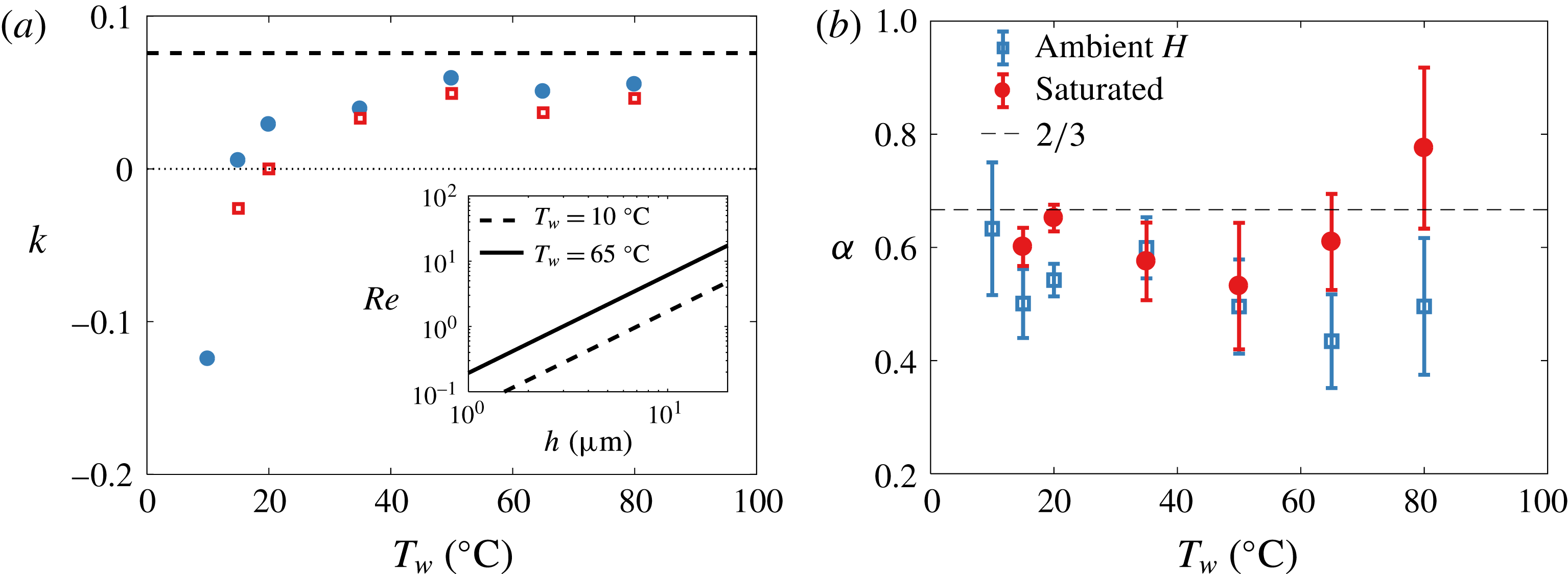
with varying water temperature for both ambient and saturated air. The curvature-driven and Marangoni flow contributions are of the same order of magnitude, both of the order of a few
 $\text{mm}~\text{s}^{-1}$
(figure 10
a inset), consistent with the physical picture presented in figure 9. These magnitudes lead to
 $Re=O(0.1{-}10)$
(figure 11
a inset), in agreement with the viscous drag posited to derive (3.6).
Figure 11(a) shows the dependence of
 $k(\unicode[STIX]{x0394}\unicode[STIX]{x1D70E})=\unicode[STIX]{x0394}h/h$
on water for both saturated and unsaturated air: the magnitude and signs are consistent with the physical picture portraying the roles of temperature gradient and evaporation in figure 9. Indeed, for a Marangoni spreading induced by surfactants that leads to marginal regeneration in soap films (Bruinsma Reference Bruinsma1995), direct experimental measurements from Nierstrasz & Frens (Reference Nierstrasz and Frens1998) show
 $k\approx 0.2$
, the same order of magnitude as what we infer in our system, but from a different origin.
(a) Plot of
 $k=\unicode[STIX]{x0394}h/h$
, leading to
 $u_{\unicode[STIX]{x0394}\unicode[STIX]{x1D70E}}=k(\unicode[STIX]{x0394}\unicode[STIX]{x1D70E})\mathit{Bo}(\unicode[STIX]{x1D70E}/\unicode[STIX]{x1D707})(h/R)^{3/2}$
. The value of
 $k$
at steady state is
 $(3\mathit{Bo})^{-1}$
(dashed line) and varies by less than
 $10\,\%$
for the range of temperature and salt concentration studied herein. Inset: Reynolds number based on
 $u_{\unicode[STIX]{x0394}\unicode[STIX]{x1D70E}}$
and taking a representative value for
 $\unicode[STIX]{x1D706}$
of 1 mm. (b) Values of
 $\unicode[STIX]{x1D6FC}$
from best fit of
 $h\sim t^{-\unicode[STIX]{x1D6FC}}$
on data shown in figures 6 and 7.
Finally, it should be noted that although
 $h\sim t^{-2/3}$
is robust at first order for the range of temperatures tested herein, we do observe an increase in noise in thickness data measurements. We can quantify the effect of increase in thickness fluctuations, in conditions in which evaporation and temperature gradients are present, with a higher-order analysis of best-fit slope
 $\unicode[STIX]{x1D6FC}$
in
 $h\sim t^{-\unicode[STIX]{x1D6FC}}$
. The mean and standard deviation of
 $\unicode[STIX]{x1D6FC}$
are shown in figure 11(b). We observe a slight deviation of
 $\unicode[STIX]{x1D6FC}$
from
 $2/3$
in part due to the increase in cap thickness inhomogeneities visible in figures 6 and 7. In the next section, we use an analogue experiment free of temperature fluctuations to test further the robustness of the proposed physical picture and generalized drainage model presented herein.
4 Analogue experiments
An 11 s old bubble in a solution of water and 2 % isopropanol volume fraction, at room temperature and humidity. (a) A particle initially present in the liquid is advected on the cap. (b) Zoom at the foot with 12.5 ms between frames showing that this particle is quickly advected towards the bubble apex after it encounters a strong localized upward flow. The maximal speed of this particle tracked along its rise is
 $0.1~\text{m}~\text{s}^{-1}$
, two orders of magnitude larger than the speeds in figure 10(a).

We now turn to analogue experiments probing the robustness of the physical picture and model proposed in § 3.2. To do so, we start by probing bubbles made of a fluid of higher volatility and lower surface tension than water. We expect that the higher the volatility is, the higher the gradient of surface tension driving upward fluid motion towards the bubble apex due to surface tension gradients induced by difference of temperature and composition between the bulk and the cap induced by evaporation will be. Figure 12 shows a bubble generated in 2 % isopropanol. The typical plumes of marginal regeneration observed on water bubbles are no longer visible, but are replaced by narrow streams of upward flow. In the series of snapshots of figure 12(b), a particle following the flow allows us to estimate an upward velocity of
 $0.1~\text{m}~\text{s}^{-1}$
, which is two orders of magnitude higher than the typical velocity of curvature-driven drainage,
 $u_{\unicode[STIX]{x0394}P}\sim O(10^{-3})~\text{m}~\text{s}^{-1}$
(figure 10(a) inset). This strikingly high upward flow strongly supports the physical picture proposed in § 3, where a dramatic shift in the drainage dynamics is expected if evaporation-induced surface tension gradients dominate. This example of isopropanol bubbles is an extreme illustration of the role of volatility driving a
 $u_{\unicode[STIX]{x0394}\unicode[STIX]{x1D70E}}$
counter to
 $u_{\unicode[STIX]{x0394}P}$
. Although smaller in magnitude due to smaller volatility, the comparison of
 $u_{\unicode[STIX]{x0394}\unicode[STIX]{x1D70E}}/u_{\unicode[STIX]{x0394}P}$
between bubbles in saturated versus unsaturated air (figures 7 and 10) clearly shows the same trend.
Thickness evolution of bubbles in fresh water and in water with
 $35~\text{g}~\text{l}^{-1}$
NaCl, showing that in unsaturated air, bubbles from the salt solution are systematically thicker than fresh water bubbles, yet follow the same law of thinning up to a certain point (a). Their thickness reaches a plateau at approximately
 $2~\unicode[STIX]{x03BC}\text{m}$
for
 $t>20~\text{s}$
, showing that they can live for considerably longer. (b) The same data represented in a log–lin scale.

(a) Bubbles in salt water (
 $35~\text{g}~\text{l}^{-1}$
) in a saturated atmosphere (left) and at ambient humidity (right), both shown at
 $t=16~\text{ s}$
. In a saturated atmosphere, the marginal regeneration patterns are similar to fresh water bubbles (figures 1
d and 8
a). At ambient humidity, evaporation strongly affects the cap dynamics. (b) A bubble in salt water (
 $35~\text{g}~\text{l}^{-1}$
) and ambient humidity at
 $t=40~\text{s}$
on which small particles, assumed to be salt crystals and highlighted with circles, are observed. (c) A 3 min old bubble in a higher concentration of salt water (
 $300~\text{g}~\text{l}^{-1}$
) and ambient humidity with 0.33 s between frames. The patterns observed are similar to those in (b). Here, one particle, a salt crystal formed on the cap, is heavy enough to slide down. The inset shows that it is surrounded by a circular meniscus. The scale bars are 1 mm and the ambient humidity is
 $H=30\,\%$
.

We now consider another analogue experiment where we probe further the physical picture discussed in § 3.2, using bubbles born from salt water. Figure 13 compares the temporal thickness evolution of bubbles emerging from salt water (deionized water with sodium chloride at
 $35~\text{g}~\text{l}^{-1}$
) with fresh water bubbles. The thinning laws obtained in a saturated environment for salt water and fresh water are near identical. Yet, significant differences emerge between bubbles in saturated and unsaturated air. In unsaturated air, the cap of salt water bubbles is consistently thicker than that of fresh water bubbles. Moreover, a striking difference emerges beyond an age of approximately 20 s, after which a peculiar thickness plateau at
 $h\simeq 2~\unicode[STIX]{x03BC}\text{m}$
is reached for salt water in unsaturated air. This plateau is associated with longer lifetimes. Indeed, while most bubbles generated in fresh water were observed to die younger than 20 s, salt water bubbles could live far longer immersed in unsaturated air: we report the thickness of bubbles as old as 3 mn in figure 13, and the oldest bubble we captured was 6 min old.
These observations support further the robustness of the physical picture of evaporation-induced Marangoni convection and the modelling developed in § 3. Here, the driver for surface tension gradient is both evaporative cooling and change in salt concentration due to evaporation. Both effects increase surface tension (figure 10
b) and lead to a decrease in cap drainage (figure 9
a). Figure 14 shows that the patterns of marginal regeneration observed on salt water bubbles in saturated ambient – i.e. without evaporation – are the same as those observed on regular fresh water bubbles. However, they are significantly disrupted for salt bubbles in unsaturated environments in which evaporation occurs. In addition, the shift in thickness profile and inhomogeneity on the bubble cap are striking for bubbles older than 20 s and falling on the thickness plateau in figure 13. Inhomogeneity in the form of two cap regions is visible (figure 14
b): the top region with minimal thickness gradient is free of marginal regeneration plumes, while the lower region remains agitated, with stronger thickness gradients. The separation between regions of distinct thickness connected by a thin transition layer is reminiscent of double-diffusion patterns. Double diffusion arises when two diffusing quantities contribute in opposite manners to the change in fluid buoyancy, which applies, for example, to salinity and temperature (Turner Reference Turner1973; Huppert & Turner Reference Huppert and Turner1981). We observed similar differences in lifetimes and cap dynamics between bubbles with a bulk concentration of
 $300~\text{g}~\text{l}^{-1}$
NaCl with and without evaporation, confirming that it is the gradient of salt concentration between the bulk water and the bubble cap, and not the high cap salt concentration alone, that alters the drainage. For long-lived salty bubbles, solid objects appear and grow on the cap (figure 14
b). When sufficiently heavy, they slide down (figure 14
c). These solid objects do not appear on salty bubbles without evaporation, or on fresh water; they are salt crystals from evaporation-induced enrichment in salt concentration on the cap.
Finally, the plateau in thickness reached for salt water bubbles in figure 13 beyond 20 s is also consistent with the mechanism we formalized in (3.8). A steady state in thickness can be reached if
 $u_{\unicode[STIX]{x0394}\unicode[STIX]{x1D70E}}=-u_{\unicode[STIX]{x0394}P}$
, a condition met for
 $k=(3\mathit{Bo})^{-1}$
. Figure 11(a) compares this value with the values of
 $k$
inferred from the temperature experiments discussed in § 3.2. They are smaller than, but close to,
 $k=(3\mathit{Bo})^{-1}$
. This shows that a small increase in surface tension gradient due to a difference in salt concentration induces a thickness plateau, in strong support of the physical picture discussed and formalized in § 3.
In sum, we have described how the film of a bubble cap empties under the concomitant action of the Laplace pressure and Marangoni stresses arising from gradient of temperature or composition. A net deterministic drainage results from this subtle balance, and the bubble cap thickness
 $h(t)$
decays in time (§ 3.2). This decay is, however, systematically interrupted when the film reaches a statistically broadly distributed, but well defined in the mean, thickness (figures 2
b, 4
d, 6, 7 and 13).
Our data and model also rationalize some of the anecdotal and scattered observations on lifetimes, some of which did report an increase in lifetime in saltwater upon decrease of relative humidity (Talmud & Suchowolskaju Reference Talmud and Suchowolskaju1931; Burger & Blanchard Reference Burger and Blanchard1983) as well as bubbles living for up to several minutes in seawater (Garrett Reference Garrett1967; Gluhosky Reference Gluhosky1983). It should be noted that while it is clear that salt delays the burst of water bubbles by affecting their drainage, Vernay et al. (Reference Vernay, Ramos, Würger and Ligoure2017) have reported that films of oil–water salty emulsions are more unstable with salt. In that case, a different bursting mechanism is at play, where the adjunction of salt can promote film bursting rather than preventing it as follows. Such an emulsified film bursts when oil droplets in its bulk reach its surface, which can be shielded from them by electrostatic repulsion in normal water. The addition of salt reduces the Debye length, therefore allowing the droplets to be closer to the interface, hence increasing the rupture probability. Drainage plays, in that scenario, no role in the first place. Nothing is known yet about the final puncture per se for the bubbles considered here, and, in particular, why the bubble cap spontaneously nucleates a hole, often close to its foot. In the remainder of the paper, we shed light on the spontaneous bubble rupture leading to bubble death (§ 5) and discuss an alternative mechanism, not relying exclusively on the presence of immiscible inclusions in the liquid (§ 6).
5 Death: ultimate film rupture
(a) Mist from the heated water interface at
 $T_{w}=65\,^{\circ }\text{C}$
visualized with schlieren imaging. A mist droplet (arrow) impacts the bubble without rupturing it. The second and third frames show the signature of the droplet on the cap 3 ms and 14 ms after impact. (b) A mist-like droplet of a solution of potassium permanganate (higher surface tension than water) impacting the water bubble without rupturing it. The frame increment is 1.4 ms. The droplets in (a) and (b) have radii of 40 and
 $55~\unicode[STIX]{x03BC}\text{m}$
and speeds of 0.2 and
 $0.7~\text{m}~\text{s}^{-1}$
respectively. (c) A pendant drop of water coalescing with the bubble cap without rupture. The frame increment is 22 ms. (d) A pendant drop of dye (
 $\unicode[STIX]{x1D70E}=55~\text{mN}~\text{m}^{-1}$
) deposited on a water bubble and rupturing it. The frame increment is 0.17 ms.

(a) Initiation of a bubble burst via a circular intrinsic cap perturbation shown with schlieren imaging. The first frame shows a floating black circular object, circled, reminiscent of microbubbles observed on the cap. The following frames, 1 s later and with increment of
 $33~\unicode[STIX]{x03BC}\text{s}$
, show the successful rupture of the film with outward capillary wave radiation. (b) Failed burst close to the foot, with frame increment of 4 ms. (c) Example of burst of a floating cap microbubble radiating capillary waves as it burst but not inducing a fatal rupture of the underlying mother bubble film. The frame increment is
 $80~\unicode[STIX]{x03BC}\text{s}$
. All bubbles are at
 $T_{w}=23\,^{\circ }\text{C}$
and the scale bars are 0.5 mm.

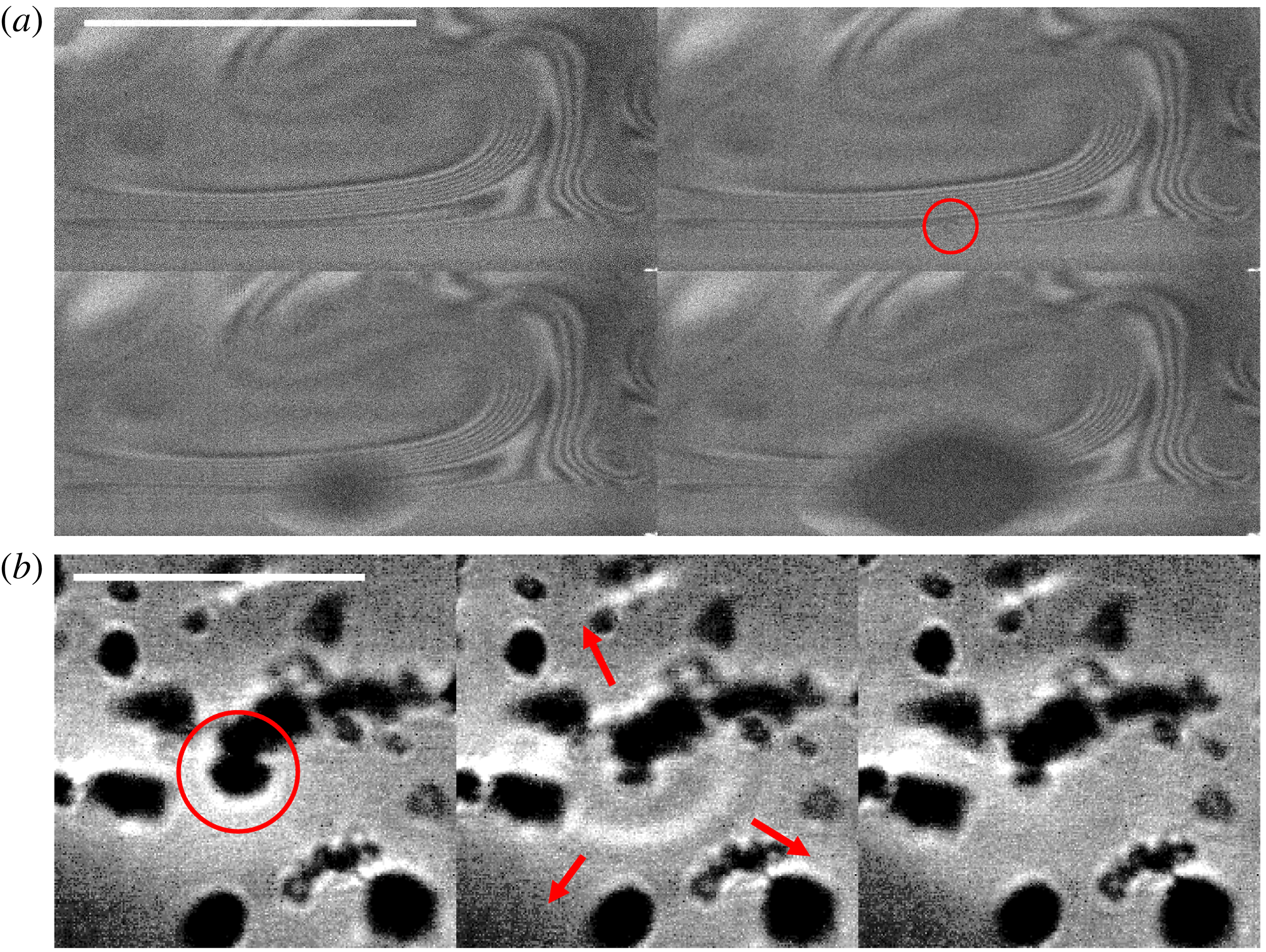
(a) Bubble burst induced by a small object (circled) rising into the cap from the bulk and crossing the thin bubble foot. The fringes are iso-thickness lines revealed by interferometry, showing the variation in film thickness around marginal regeneration plumes. The scale bar is 0.5 mm and the frame increment is
 $50~\unicode[STIX]{x03BC}\text{s}$
. The bubble killer is aspherical, and thus could be either a particle or a microbubble surrounded with particles, as illustrated in (b) using schlieren imaging. There,
 $T_{w}=97\,^{\circ }\text{C}$
, the water is dirty, and spherical microbubbles and aspherical particles are seen. The microbubble circled in red carries aspherical particles and is seen bursting without rupturing the cap. The frame increment is
 $67~\unicode[STIX]{x03BC}\text{s}$
and the scale bar is 1 mm.
We have observed a correlation between lifetimes and thicknesses: thicker bubbles are more resistant to burst than thinner ones and, on average, live for longer. This might appear intuitive given that thermal fluctuations and van der Waals forces are known to destabilize nanometre-thin films (Vrij Reference Vrij1966; Israelachvili Reference Israelachvili2011). The extensive lifetime and cap thickness measurements that we have presented in prior sections show that below thicknesses of 0.5–
 $1~\unicode[STIX]{x03BC}\text{m}$
, the film ruptures and bubbles are unlikely to survive. However, (1) this is thicker than the nanometre scale at which van der Waals forces and thermal fluctuations dominate, and (2) the likelihood of film rupture and bubble death is distributed: at higher thicknesses of the order of 1–
 $10~\unicode[STIX]{x03BC}\text{m}$
, bubbles can still rupture. Ultimately, it is a combination of deterministic thinning and a range of stochastic events that shapes the final death of bubbles. Next, we discuss a series of bubble-killing mechanisms from external perturbations, such as impacts, to particles or microbubbles intrinsically present in non-highly-purified water. We finish by presenting a very efficient mechanism that can enhance all others in addition to being intrinsically coupled with the mixing of the bubble cap.
5.1 Extrinsic perturbations
External perturbations from violent airflow, or violent impacts of particles or droplets (Taylor & Michael Reference Taylor and Michael1973), were reported to rupture thin films. Although this is true for extreme events, we did not observe bubble rupture readily upon impact of regular mist water droplets (figure 15 a) and found that mean lifetime trends (figure 4 a) are not distinct when shielding bubbles from mist. Impacts by mist-like drops of higher surface tension than that of water did not alter the cap either (figure 15 b). However, localized decrease of surface tension associated with such external impacts can be strikingly efficient at rupturing the film: figure 15(c,d) compares contact and coalescence events with pendant drops of (c) pure water and (d) dyed water. Dye locally reduces surface tension, creating a diverging flow sufficient to rupture the cap. When the drop is made of pure water, non-fatal coalescence occurs instead.
5.2 Localized intrinsic perturbations: particles and microbubbles
Internal inhomogeneities in the form of particles or other inclusions can rupture the film, simply inducing an additional local thinning of the cap. Hydrophobic particles are discussed extensively in the literature (de Gennes Reference de Gennes1998), but we also observed other inclusions. Figure 16(a) shows the presence of a spherical object on the cap which induces lethal rupture. Preceding the hole opening, a transition in the small inclusion occurs: it appears to burst and emit capillary waves. That burst is then followed by the cap rupture. The appearance of burst and sphericity of the object shows that this object is a microbubble floating on the mother bubble cap. Figure 16(c) shows another cap where the microbubble bursts and emits capillary waves. However, the disturbance from this burst is not sufficient to rupture the mother bubble. We readily saw such microbubbles accumulate at the foot or climb up the cap of the mother bubbles. Their number increases as we increase water temperature, as expected from inhomogeneous bubble nucleation in the nano- or microcrevasses of tube walls (Carey Reference Carey2007). Using interferometry, we reveal such microbubbles and other objects intrinsic to dirty water.
(a,b) Electrolysis microbubbles produced in the bulk water and (c) their appearance on the bubble cap visible with schlieren visualization. The scale bars are 1 mm. The circled bubbles are
 $170~\unicode[STIX]{x03BC}\text{m}$
in radius. (d) Bubble lifetime before and during electrolysis. After electrolysis is turned on (vertical line), bubbles live for shorter times on average; the solid line is the moving average.

Figure 17(a) reveals the interferometric iso-thickness lines connecting the bubble foot to one of the rising plumes of marginal regeneration. The circled object passing through the constricted region causes the rupture of the mother bubble film. The object revealed is not perfectly spherical; it is an example of a particle, or possibly microbubble carrying particles with it. Indeed, figure 17(b) shows a zoomed view of a dirty bubble cap using schlieren imaging where spherical objects, microbubbles, are connected to aspherical objects, presumably simply due to capillary attraction. Although we saw myriads of bursts induced by such ubiquitous objects, we also saw them floating on caps (or even bursting) without causing lethal ruptures (e.g. figure 16 b,c). Hence, it remains unclear how they interact with the cap film and what sets their efficiency in killing the mother bubble. We quantify their influence on bubble lifetime by adding intrinsic microbubbles to the mother bubble in a controlled manner using electrolysis.
Figure 18(a,b) shows the two electrodes added to the water and the myriad of microbubbles with typical sizes proportional to the wire roughness. A large number of microbubbles appear on the cap of the emerging bubbles when electrolysis is on. Figure 18(c) is an example in which we slightly stabilized the mother bubble (minute amount of soap) to illustrate the high density of microbubbles climbing and bursting on it. For pure water bubbles without soap, the bubbles had low resistance to the many bursts and had very short lifetimes. This is quantified in figure 18(d), where it is clear that the introduction of microbubbles onto surface bubbles decreases their lifetime.
In sum, microbubbles and particles floating in most non-ultra-purified waters can cause the final rupture of surface bubbles even when they are thick. Clearly, intrinsic perturbations are more efficient and ubiquitous bubble killers than the extrinsic impacts from mist or violent airflow discussed in § 5.1. Moreover, the thicker the bubble is, the more likely it is to live longer, on average. As a bubble ages and thins down to 0.5–
 $1~\unicode[STIX]{x03BC}\text{m}$
, intrusions are likely to locally reduce the film thickness sufficiently for van der Waals or thermal fluctuations to cause rupture. However, our observations also show that intrinsic perturbations, such as microbubbles and particles, or extrinsic perturbations, such as impacts, are not equal in their efficiency to kill thick bubbles. Next, we discuss the missing ingredient that can systematically enhance this efficiency.
A water bubble at
 $T_{w}=10\,^{\circ }\text{C}$
just after it emerges from the water surface. (a) A thinning region developing close to the bubble apex (2.7 ms between frames). (b) The bubble eventually bursts when a hole nucleates in this region. The anisotropy of the rim illustrates the low thickness (1–10 nm) of this region compared with the rest of the cap (
 $1{-}10~\unicode[STIX]{x03BC}\text{m}$
). The scale bar represents 1 mm and
 $\unicode[STIX]{x0394}\unicode[STIX]{x1D70E}=\unicode[STIX]{x1D70E}(T_{a})-\unicode[STIX]{x1D70E}(T_{w})=1.9~\text{mN}~\text{m}^{-1}$
.

5.3 Localized Marangoni-driven violent death
(a) A needle at room temperature,
 $T_{a}=23\,^{\circ }\text{C}$
, approaching a bubble at
 $T_{w}=15\,^{\circ }\text{C}$
. (b) Zoom on the zone close to the needle, with
 $14~\unicode[STIX]{x03BC}\text{s}$
between frames. The star indicates the first frame on which we observe the burst. Here,
 $\unicode[STIX]{x1D70E}(T_{w})-\unicode[STIX]{x1D70E}(T_{a})=1.2~\text{mN}~\text{m}^{-1}$
. A similar pattern and puncture initiation is observed when (c) a hot stick (
 $\unicode[STIX]{x0394}\unicode[STIX]{x1D70E}\sim 10~\text{mN}~\text{m}^{-1}$
) or (d) an isopropanol droplet (
 $\unicode[STIX]{x0394}\unicode[STIX]{x1D70E}\sim 50~\text{mN}~\text{m}^{-1}$
) approaches a bubble at room temperature. Scale bars are 1 mm.

Bubbles in cold water live for a shorter time and are thinner than bubbles in hot water (figures 4 and 6). In fact, we observed that a large number of cold bubbles (
 $T_{w}=10\,^{\circ }\text{C}$
) burst immediately upon surfacing. Close inspection reveals distinct patterns on the cap preceding these bursts. Figure 19 shows an extended area of thin film that eventually ruptures, showing a localized low thickness of 1–10 nm, scales at which van der Waals forces can act. These patterns, frequently observed when the air is significantly hotter than the bulk water, are reminiscent of locally diverging Marangoni fronts (e.g. figure 15
d).
We also observed such patterns when approaching a needle (speed
 ${\sim}0.2~\text{m}~\text{s}^{-1}$
, base diameter 0.37 mm) hotter than the bubble cap. The needle motion induces airflow towards the cap as it approaches, with circular patterns similar to those naturally occurring in figure 19. In figure 20(a,b), the pattern onset precedes establishment of contact between the needle and the bubble. In addition, the pattern develops and widens for more than
 $770~\unicode[STIX]{x03BC}\text{s}$
, while the ultimate rupture of the film, when it finally occurs (starred snapshot), lasts for less than
 $14~\unicode[STIX]{x03BC}\text{s}$
. We are able to reproduce such patterns also by approaching a heated metal needle or a drop of isopropanol (figure 20
c,d) close to the bubble cap. In both cases, the perturbation (source of heat or isopropanol fumes) remains distant and no direct contact occurs with the cap prior to the onset of patterns and cap rupture.
In all of the above cases presented in figure 20, the patterns on the cap are strikingly similar and analogous to those in figure 19. They are characterized by two stages: a first stage of development of concentric patterns and a second stage of rapid final rupture. Clearly, the thermal or chemical perturbation of the interface induces local reduction of surface tension associated with highly efficient local film thinning. We also observed such a two-step process of rupture at the foot of bubbles naturally bursting at ambient temperature, such as in figure 21. Although not always observed in association with the microbubbles or particles discussed in § 5.2, such divergent Marangoni thinning is strikingly efficient at rupturing the cap. Its coupling with microbubbles or particles would dramatically increase their efficiency in rupturing thick bubbles. In fact, minute fluctuations of composition of the atmosphere around the bubble cap, any aerosol coalescing with it or any immiscible droplet or microbubble in the liquid smearing the film with traces of pollutants can locally change the liquid chemical or thermal composition.
We test further the extent of this effect with controlled needle piercing of the bubbles at various temperatures. Figure 22 compares the thickness measurements, obtained via the Taylor–Culick speed of rupture of the cap, from natural bursts and triggered bursts. The metal needle was at ambient air temperature,
 $T_{a}=23\,^{\circ }\text{C}$
, and moved into the film at various ages of the bubbles. A clear distinction is visible between the thicknesses measured for naturally bursting bubbles and those triggered for all temperatures, except at ambient water temperature (figure 22
b). In this last case, the water bubble and the needle have the same temperature. Moreover, the thickness difference between the needle-triggered and natural bursts shifts as the cap temperature increases from being cooler (figure 22
a) to being hotter than the needle (figure 22
c,d). These thickness measurements are consistent with a highly efficient localized Marangoni-driven thinning (
 $T_{cap}<T_{needle}$
) or thickening (
 $T_{cap}>T_{needle}$
) the cap. It should be noted how such needle localized perturbations affect the measurement of thickness
 $h$
. Hence, care is needed when interpreting the relationship between the thickness of a film and its rupturing speed when the film is pierced using surface-active perturbations such as heat (Petit, Le Merrer & Biance Reference Petit, Le Merrer and Biance2015) or ethanol (Sabadini, Ungarato & Miranda Reference Sabadini, Ungarato and Miranda2014). For
 $h\sim 0.5{-}1~\unicode[STIX]{x03BC}\text{m}$
, the bubbles are thin enough that even less efficient mechanisms such as non-Marangoni-driven intrinsic intrusions (microbubbles or particles) can locally thin the film further for van der Waals forces and thermal fluctuations to be able to act. In the next section, we formalize the mechanism that best captures lethal rupture.
Natural two-stage burst at the foot of a thick bubble in ambient temperature
 $23\,^{\circ }\text{C}$
. (a) The initial phase of dark concentric pattern deepening for more than
 $100~\unicode[STIX]{x03BC}\text{s}$
before rupturing in less than
 $33~\unicode[STIX]{x03BC}\text{s}$
in (b). Images were taken with
 $33~\unicode[STIX]{x03BC}\text{s}$
between each frame and a scale bar of 0.5 mm. (b) The burst that is triggered with
 $800~\unicode[STIX]{x03BC}\text{s}$
between each frame and a scale bar of 2 mm. The last frame in (a) corresponds to the first frame in (b).

6 Criteria for puncture
6.1 Physical picture
We discuss a mechanism that captures the body of observations on lethal rupture presented so far. We recall that (1) we observed that among all reported perturbations (from drop impact to microbubble or particle inclusion), the ones involving or coupled with a Marangoni thinning are the most lethal and efficient in rupturing the cap (figures 19–22); (2) we observed a number of failed cap bursts where it appeared that only one side of the film was perturbed, but then healed (figure 16 b,c); (3) we observed that time is required for the rupture of the film and that such time is associated with apparent deepening of the perturbation until the other side of the film ruptures (e.g. figure 21); finally (4) we observed that most bursts occur at the foot of the bubble even when the perturbation is introduced and is stirred on the cap (figure 23). This last observation has been previously reported (e.g. Lhuissier & Villermaux Reference Lhuissier and Villermaux2012), and in our approximately 900 direct observations of spontaneous bursts, we observed that more than 80 % of them occurred in the direct vicinity of the foot.
Given these observations, we propose a mechanism of fatal bubble rupture. Surfactants in minute quantities are necessary to sustain a bubble, which is a metastable film. They reside typically at the interface of the film and are responsible for its stirring via marginal regeneration on the cap (e.g. figure 1 d). Considering the bubble drainage discussed in § 3, insoluble surfactants accumulate, on average, at the bubble foot. Soluble impurities can be transported by insoluble surfactants themselves, or by other intrinsic inclusions (e.g. particles or microbubbles in § 5.2) or extrinsic perturbations (e.g. dust or drop impacts in § 5.1).
Comparison of the measured thickness evolution for natural rupture of the bubble cap and punctures triggered by a fast stainless steel needle at room temperature,
 $T_{a}=23\,^{\circ }\text{C}$
, for different water temperature
 $T_{w}$
: (a)
 $15\,^{\circ }\text{C}$
, (b)
 $23\,^{\circ }\text{C}$
, (c)
 $35\,^{\circ }\text{C}$
and (d)
 $50\,^{\circ }\text{C}$
. The inset in (d) shows that when the bubble cap is hotter than the needle, the needle does not always succeed in rupturing the cap. Upon failure to rupture, a thick patch of fluid is left behind. The scale bar is 1 mm, with 2.67 ms between frames. The lines are guides to the eye.

We propose that contaminant-induced lethal rupture can only occur when a soluble surfactant blob of size
 $a$
can diffuse across the film of thickness
 $h$
and initiate lethal Marangoni thinning on both sides of the film. To operate, this mechanism must have time to develop, and we argue that this is more likely at the foot rather than on the cap due to two effects. First, the foot is thinner than the cap and is the location of accumulation of insoluble surfactants, leading to local transverse shear that can assist transverse diffusion. Second, stirring and mixing along the cap is more efficient than transverse diffusion through the cap, lowering the probability of successful side-to-side penetration and Marangoni opening on the cap. Next, we derive the criteria for such impurities to have time to diffuse through the entire film before diffusing along the cap, or draining out of it.
(a) A blob smaller than
 $50~\unicode[STIX]{x03BC}\text{m}$
, first detected at the top of a
 $13~\unicode[STIX]{x03BC}\text{m}$
-thick dirty bubble cap, is tracked. Red dots correspond to its position every 31 ms as it is drained. Only when it reaches the bubble foot does it puncture the cap, very quickly. (b) Zoom close to the region where the burst occurs (left to right, top to bottom). The first frame highlights the blob just before it reaches the bubble foot. The second frame, 32 ms latter, shows the blob in the foot (white) before the nucleation of a hole
 $66~\unicode[STIX]{x03BC}\text{s}$
later. Scale bars are 1 mm.

6.2 Transverse contamination: time-scale competition in cap versus foot
A soluble blob of surfactant of size
 $a$
diffuses from one side of the film, of thickness
 $h$
, to the other side, over a time
 $\unicode[STIX]{x1D70F}_{diff}\sim h^{2}/D$
, where
 $D$
is the diffusion coefficient. Here, we define a blob as an area or volume of inhomogeneity in or on the cap. The same blob typically diffuses longitudinally along the cap over a time
 $a^{2}/D$
. The competition of these two time scales determines whether the contaminant can rupture the film of thickness
 $h$
on both sides faster than its dilution along the cap. At first order, this criterion reduces simply to
 $h<a$
. In § 6.4, we return to longitudinal cap stirring time scales and show that side-to-side diffusion is disadvantaged on the cap even when this simple criterion is satisfied.
Now, we consider the foot of the bubble. First, it is typically, at most, twice as thin as the cap, leading to a time scale of side-to-side diffusion that is
 ${\sim}h^{2}/4D$
and, hence, an efficient side-to-side rupture for
 $h<2a$
. A perturbation of size
 $a$
can rupture, on both of its film sides, a bubble cap thicker than
 $2a$
if such perturbation is at the foot rather than on the cap. In addition to this simple geometric argument, a second constraint governs the foot. In the marginal regeneration region, the film interface is rigidified by surfactants accumulated by drainage, leading to local no-slip at the interfaces. Hence, a shear across the film can develop, with intensity
 $u/\unicode[STIX]{x1D6FF}$
, where
 $\unicode[STIX]{x1D6FF}$
is the shear layer thickness (figure 24). Such transverse shear can enhance diffusion of soluble contaminant across the film, similarly to classical shear-enhanced transfer in boundary layers (Lévêque Reference Lévêque1928; Landau & Lifshitz Reference Landau and Lifshitz1959). We use this analogy to derive other time scales, the competition of which ensures timely side-to-side contamination and associated lethal film rupture.
Figure 24 illustrates the analogy of double boundary layers and shear-enhanced transfer of contaminant of concentration
 $C$
in a film of thickness
 $h$
, and where
 $\unicode[STIX]{x1D6FF}$
sets the shear intensity while
 $\unicode[STIX]{x1D6FF}^{\prime }$
sets the contaminant flux. Given flux conservation, the time scale
 $T$
needed for side-to-side penetration of the contamination is
 $$\begin{eqnarray}\displaystyle h\frac{C}{T}\sim D\frac{C}{\unicode[STIX]{x1D6FF}^{\prime }}\quad \text{or}\quad T\sim \frac{h\unicode[STIX]{x1D6FF}^{\prime }}{D}. & & \displaystyle\end{eqnarray}$$
(a) Schematic of shear-enhanced mixing of contaminant from surface deposition to film depth at the bubble foot. The contaminant of size
 $a$
(red) drains down to the bubble foot, where shear enhances its diffusion across the film to the other side of the cap film. (b) Schematic velocity (
 $u$
, solid line) and concentration of contaminant (c, dashed line) profiles in the bubble foot. Here,
 $\unicode[STIX]{x1D6FF}$
is the thickness of the momentum shear layer and
 $\unicode[STIX]{x1D6FF}^{\prime }$
is the thickness of the boundary layer of concentration.

Neglecting longitudinal diffusion along the
 $x$
-direction of the mean flow
 $u$
, the shear-assisted transverse diffusion of
 $C$
is governed by
 $$\begin{eqnarray}\displaystyle u(y)\frac{\unicode[STIX]{x2202}C}{\unicode[STIX]{x2202}x}=D\frac{\unicode[STIX]{x2202}^{2}C}{\unicode[STIX]{x2202}y^{2}},\quad \text{with }u(y)\sim u\frac{y}{\unicode[STIX]{x1D6FF}}, & & \displaystyle\end{eqnarray}$$
where
 $y$
is the direction normal to the mean flow
 $u$
(figure 24). For long molecules of surfactants in water, we expect a high momentum versus mass transfer, leading to a large Schmidt number
 $\mathit{Sc}=\unicode[STIX]{x1D708}/D\sim O(10^{4})$
. Hence, we expect
 $\unicode[STIX]{x1D6FF}^{\prime }<\unicode[STIX]{x1D6FF}$
, as illustrated in figure 24(b). In this limit, the classical problem of heat or mass transfer across the boundary layer (Lévêque Reference Lévêque1928; Landau & Lifshitz Reference Landau and Lifshitz1959) leads to
 $$\begin{eqnarray}\displaystyle \unicode[STIX]{x1D6FF}^{\prime }\sim \unicode[STIX]{x1D6FF}\mathit{Sc}^{-1/3}. & & \displaystyle\end{eqnarray}$$
Combination of (6.1) and (6.3) allows us to re-express the transverse contaminant shear-enhanced diffusion time scale in the bubble foot as
 $$\begin{eqnarray}\displaystyle T\sim \frac{h\unicode[STIX]{x1D6FF}}{D}\mathit{Sc}^{-1/3}. & & \displaystyle\end{eqnarray}$$
For side-to-side penetration, either the purely diffusive,
 $h^{2}/D$
(in the cap), or the shear-enhanced diffusive,
 $T$
(in the foot), time scale should be shorter than the contaminant residence time,
 $\unicode[STIX]{x1D70F}=R^{2}/u\ell _{c}$
(3.2), on the bubble. Typically,
 $h^{2}/D>T$
. Thus, side-to-side penetration needed for onset of fatal rupture can occur if
 $$\begin{eqnarray}\displaystyle T<\unicode[STIX]{x1D70F}. & & \displaystyle\end{eqnarray}$$
If this is satisfied, the minimal size
 $a$
of a contaminant blob that has the potential to penetrate the film side to side, hence causing rupture, is such that
 $a^{2}/D>T$
, or
 $$\begin{eqnarray}\displaystyle a>\sqrt{h\unicode[STIX]{x1D6FF}^{\prime }}. & & \displaystyle\end{eqnarray}$$
Given
 $\mathit{Sc}\sim O(10^{4})$
,
 $a$
corresponds to a fraction of the film thickness at burst
 $h_{b}=O(\unicode[STIX]{x03BC}\text{m})$
, the exact value of which is set by the foot shear intensity, i.e. by
 $\unicode[STIX]{x1D6FF}$
.
6.3 Marangoni-induced condition of film rupture
Once the contaminant is introduced or reaches one interface of the film at concentration
 $C$
, leading to a local surface tension deficit
 $\unicode[STIX]{x0394}\unicode[STIX]{x1D70E}$
, rupture can occur if the time scale of self-sustained Marangoni-induced divergence and thinning is shorter than
 $a^{2}/D$
. This condition can be shown to reduce to (Néel & Villermaux Reference Néel and Villermaux2018)
 $$\begin{eqnarray}\displaystyle \frac{a^{2}}{D}>\sqrt{\frac{\unicode[STIX]{x1D70C}a^{2}h}{\unicode[STIX]{x0394}\unicode[STIX]{x1D70E}}}. & & \displaystyle\end{eqnarray}$$
On a bubble draining at quasi-mechanical equilibrium, the difference of surface tension between the top of the cap and the bubble foot is
 $\unicode[STIX]{x0394}\unicode[STIX]{x1D70E}\sim \unicode[STIX]{x1D70E}h/R=O(10^{-1}{-}10^{-2})\,\text{mN}\,\text{m}^{-1}$
for
 $R=O(\ell _{c})$
and
 $h=O(10^{-5}-10^{-6}~\text{m})$
(Lhuissier & Villermaux Reference Lhuissier and Villermaux2012). Assuming that this surface tension deficit is comparable to that induced by a soluble contaminant of size
 $a$
, (6.7) becomes
 $$\begin{eqnarray}\displaystyle a>D\sqrt{\frac{\unicode[STIX]{x1D70C}R}{\unicode[STIX]{x1D70E}}}, & & \displaystyle\end{eqnarray}$$
leading to
 $a\gtrsim 10~\text{nm}$
. This condition is much less restrictive than
 $a\gtrsim h$
and suggests that even very small impurities have the potential to induce rupture.
Mixing on a bubble cap. (a) A drop of potassium permanganate is gently deposited at the surface of a bubble just formed. It is soon converted into a set of lamellae, elongating and overlapping in an ever weakening stirring field. At the time of burst, the dye has been spread out all over the cap, with very weak residual concentration fluctuations. The snapshots show when the drop is deposited (
 $t=-0.3~\text{s}$
),
 $t=0$
(corresponding to the time at which most of the patch of deposited potassium permanganate has drained) and times
 $0.5$
,
 $0.75$
, 1.3 s before burst and 1.3 s during burst. The scale bar is 2 mm. (b) Concentration distribution
 $p(c)$
of the dye in the late stages of the mixing process on the bubble cap. It is represented by (6.11) and narrows around the mean at a pace
 $n=(t/t_{s})^{3/2}$
(inset), with
 $t_{s}=0.15~\text{s}$
the mixing time of the dye.

6.4 Mixing on the cap
We return to the cap dynamics. Side-to-side penetration on the cap requires the time scale of diffusion through the film to be smaller than the mixing time
 $t_{s}$
of the contaminant blob longitudinally to the cap surface. Figure 25 shows that this is not likely to occur on the upper part of the bubble cap, where efficient stirring and mixing is driven by longitudinal agitation from marginal regeneration plumes. We recall the curvature-induced cap velocity
 $u_{\unicode[STIX]{x0394}P}\sim (\unicode[STIX]{x1D70E}/\unicode[STIX]{x1D707})(h/R)^{3/2}$
(§ 3.1) and the typical size of plumes
 $\unicode[STIX]{x1D706}\sim R(h/R)^{3/2}$
(§ 3.2). The stirring by marginal regeneration plumes induces elongation of material lines at a rate
 $\unicode[STIX]{x1D6FD}=u_{\unicode[STIX]{x0394}P}/\unicode[STIX]{x1D706}\sim \unicode[STIX]{x1D70E}/\unicode[STIX]{x1D707}R$
. The elongation rate
 $\unicode[STIX]{x1D6FD}$
is independent of time, so that a blob of initial size
 $a$
projected on the cap soon becomes a lamella of length
 $\unicode[STIX]{x1D702}=a(1+\unicode[STIX]{x1D6FD}t)$
. The stretching rate of the blob
 $\dot{\unicode[STIX]{x1D702}}/\unicode[STIX]{x1D702}$
is such that
 $$\begin{eqnarray}\displaystyle \frac{\dot{\unicode[STIX]{x1D702}}}{\unicode[STIX]{x1D702}}\xrightarrow[{\unicode[STIX]{x1D6FD}t\gg 1}]{}\frac{1}{t}, & & \displaystyle\end{eqnarray}$$
decaying in time proportionally to the residence time
 $\unicode[STIX]{x1D70F}$
in (3.2). Thus, the mixing time of the blob is (Villermaux Reference Villermaux2012)
 $$\begin{eqnarray}\displaystyle t_{s}=\unicode[STIX]{x1D6FD}^{-1}\mathit{Pe}_{a}^{1/3},\quad \text{with }\mathit{Pe}_{a}=\frac{\unicode[STIX]{x1D6FD}a^{2}}{D} & & \displaystyle\end{eqnarray}$$
the Péclet number based on the blob size
 $a$
. The mixing time
 $t_{s}$
soon becomes smaller than the age of the bubble
 $t$
, consistent with our observation of short cap mixing time scale of blobs even when their initial size is comparable to that of the bubble (figure 25).
After
 $t_{s}$
, the stretching rate of the blob progressively weakens and the transverse width of the lamellae concentration profile increases as
 $\sqrt{Dt}$
. The surface occupied by the blob thus increases as
 $a\unicode[STIX]{x1D6FD}t\sqrt{Dt}\sim t^{3/2}$
, and the mean concentration of pollutant that it carries decays inversely proportionally to it. As the lamellae evolve on a finite area, they necessarily eventually overlap. After
 $n$
overlaps, the contaminant concentration distribution
 $p(c)$
on the cap is (Villermaux & Duplat Reference Villermaux and Duplat2003)
 $$\begin{eqnarray}\displaystyle p(c=C/\langle C\rangle )=\frac{n^{n}}{\unicode[STIX]{x1D6E4}(n)}c^{n-1}e^{-nc}, & & \displaystyle\end{eqnarray}$$
with
 $n\sim t^{3/2}$
, since the average concentration
 $\langle C\rangle$
of the mixture is assumed to be approximately constant throughout the life of the bubble. Figure 25 shows that a blob of potassium permanganate, a substance soluble in water passively advected on the cap, indeed mixes according to (6.11), with the anticipated time dependence on
 $n$
. The mixing time of this dye, found to be
 $t_{s}\approx 0.15~\text{s}$
, is much smaller than the bubble lifetime of approximately 1.5 s, and concentration fluctuations are appreciably erased by time of burst. In sum, stirring is too efficient on a bubble cap to allow for contamination throughout the film thickness. This, coupled with the shear-enhanced side-to-side diffusion mechanism discussed in § 6.2, supports our observation that bubbles seldom nucleate holes on the surface of their cap, as opposed to their foot (e.g. figures 23 and 25).
6.5 Robustness of burst physical picture and thickness at burst
Thus far, we have rationalized our observations of bubble death in terms of competition of time scales promoting rupture at the foot via Marangoni self-sustained divergence that occurs on both sides of the film interface. We probe further the robustness of the physical picture and formalism introduced in this section via its consistency with prior observations on bubble bursting.
In the case of a shear layer in the foot of length scaling as
 $\unicode[STIX]{x1D6FF}\sim \unicode[STIX]{x1D708}/u$
(figure 24),
 $T$
reduces to
 $T\sim \mathit{Sc}^{2/3}h/u\sim t^{1/3}$
from (6.4), while the drainage time scale remains
 $\unicode[STIX]{x1D70F}\sim R^{2}/u\ell _{c}\sim t$
(§ 3.1). Thus, the duration of residence on the bubble,
 $\unicode[STIX]{x1D70F}$
, increases faster with time than the foot shear-enhanced side-to-side diffusion time scale
 $T$
: the condition (6.5) for fatal rupture is eventually fulfilled. Moreover, both
 $\unicode[STIX]{x1D70F}$
and
 $T$
are inversely proportional to the mean drainage velocity
 $u$
. Hence, the rupture criterion (6.5) is robust to change in
 $u$
introduced by the coupling of the bubble to its environment discussed in § 3. As a bubble ages, (6.5) is first met for a critical thickness
 $h_{b}$
,
 $$\begin{eqnarray}\displaystyle h_{b}=\frac{R^{2}}{\mathit{Sc}^{2/3}\ell _{c}}, & & \displaystyle\end{eqnarray}$$
which is essentially (1.1) with the origin of
 ${\mathcal{L}}$
now established:
 ${\mathcal{L}}=\ell _{c}\mathit{Sc}^{2/3}$
. In fact, for weakly diffusing impurities in water,
 $\mathit{Sc}=O(10^{4})$
and
 ${\mathcal{L}}=O(1~\text{m})$
. Recalling (3.3), the expected bursting time of a bubble now reads as
 $$\begin{eqnarray}\displaystyle t_{b}=t_{v}\mathit{Sc}\left(\frac{R}{\ell _{c}}\right)^{1/2}, & & \displaystyle\end{eqnarray}$$
with a correction factor
 $(1/3-k\mathit{Bo})^{-1}$
needed when using the thickness evolution accounting for Marangoni effects (3.8). This expression recovers the dependences in
 $R,\ell _{c}$
and
 $t_{v}$
of (1.3), and is now also completed with a dependence on
 $\mathit{Sc}$
: if a contaminant cannot diffuse fast enough across a film (
 $\mathit{Sc}\rightarrow \infty$
), rupture cannot occur.
It should be noted that, all else being equal, an increase in dynamic viscosity
 $\unicode[STIX]{x1D707}$
is expected to decrease the diffusion coefficient
 $D$
, with
 $D\sim 1/\unicode[STIX]{x1D707}$
according to the Einstein–Sutherland law, and hence to increase the lifetime as
 $t_{b}\sim \unicode[STIX]{x1D707}^{3}$
. The lifetime can also eventually become larger than the pure diffusion time across the film
 $\unicode[STIX]{x1D70F}_{diff}\sim h_{b}^{2}/D$
since
 $$\begin{eqnarray}\displaystyle \frac{t_{b}}{\unicode[STIX]{x1D70F}_{diff}}=\frac{\unicode[STIX]{x1D708}\unicode[STIX]{x1D707}}{\unicode[STIX]{x1D70E}\ell _{c}}\left(\frac{R}{\ell _{c}}\right)^{-7/2}\mathit{Sc}^{4/3}, & & \displaystyle\end{eqnarray}$$
especially for bubbles with radius
 $R$
substantially smaller than the capillary length
 $\ell _{c}$
. However, this discussion must not be limited to the temperature or other water parameter dependences of kinetic coefficients. Indeed, such change in
 $t_{b}$
is independent of the change in drainage, which can itself be slowed down by the intensity of Marangoni flows, as we have shown in (3.8). As seen in § 2, in that context, this last effect is dominant for setting the lifetime distribution data obtained from experiments with distinct water properties and in distinct environmental conditions.
Finally, it should be noted that all time scales proposed in § 6 are scalings reflecting dependences on key drainage and contamination variables. It is the comparison of these time scales within the same level of accuracy, rather than their absolute values, that led us to criteria finally leading to (6.13) and that are consistent with an extensive body of observations on surface bubble ageing and bursting from our present study and those of others conducted over the past decades. Precise and direct measurements of some of the time scales and length scales discussed, such as those associated with shear-enhanced diffusion, mixing and stirring within and along the cap and the foot, would be required for a precise estimate of lifetime given a set of water and air conditions. These would require analogue experiments carried out in extremely well controlled conditions and focusing on the dynamics of inclusions of known chemical properties in thin films.
7 Discussion
We have presented the results of a combined theoretical and experimental investigation of the life, ageing and burst of surface bubbles, with a particular focus on relatively large bubbles producing film droplets. An understanding of what shapes the sizes and payloads of these droplets in a range of indoor and outdoor environments starts by understanding the fundamental physics of birth, drainage and burst of their mother bubble. We investigated the role of water source, temperature, salinity and surrounding air moisture on the lifetime and thinning of bubbles, as well as on the conditions favouring their final fatal rupture when they are relatively thick. Bubbles in hot water were found to live for longer, on average, than in cold water, contrary to what would have been expected from prior models of bubble drainage and lifetime (§ 2). Moreover, we found that mean lifetimes alone are not sufficient to characterize a population of bubbles; the whole lifetime distribution must be provided to identify in which regime bubbles burst. The mean and distribution of lifetimes are the result of a complex interplay between bubble thickness and drainage, and the mechanisms triggering final rupture. We thus moved on to examine thinning and burst separately.
We showed that although their thickness
 $h$
continues to follow a robust
 $h\sim t^{-2/3}$
law, hot bubbles are actually thicker than their colder counterparts of the same age. Similarly, bubbles in ambient air are thicker than bubbles of the same age in saturated air. Both findings are counter to the expected increase of evaporative water removal from the cap. In fact, this effect remains negligible overall over bubble lifetimes of the order of 1–20 s, while surface tension gradients induced by thermal or evaporative cooling establish a counterflow that can act against curvature-driven drainage. This physical picture is formalized in the form of a generalized drainage model (§ 3) accounting for the concomitant action of the Laplace pressure and an additional flow induced by local thinning from Marangoni stresses:
 $u_{\unicode[STIX]{x0394}\unicode[STIX]{x1D70E}}\sim k(\unicode[STIX]{x0394}\unicode[STIX]{x1D70E})\mathit{Bo}(\unicode[STIX]{x1D70E}/\unicode[STIX]{x1D707})(h/R)^{3/2}$
(3.6). We demonstrated the robustness of this physical picture and model with additional experiments involving volatile liquids and salt water (§ 4). The illustration of the proposed mechanism can be dramatic. For example, salty bubbles in unsaturated air are thicker than those in saturated air throughout their life, and their drainage can even halt. This halt, associated with a plateau of thickness, is also captured by our generalized drainage model. Bubbles reaching it can live for minutes rather than seconds and become enriched in salt to the point of salt crystal formation (figure 14).
The net deterministic drainage is systematically interrupted when the film reaches a statistically broadly distributed, but well defined in the mean, thickness. Although we observed a correlation between lifetime and thickness – thicker bubbles appear on average to be more resistant to burst than thinner ones – they burst at thicknesses of the order of 1–
 $10~\unicode[STIX]{x03BC}\text{m}$
, much larger than the nanometre scale at which van der Waals forces and thermal fluctuations dominate. We turned to an extensive study of the final puncturing mechanisms to elucidate why bubbles, even when thick, spontaneously nucleate a hole (§ 5). We reported fatal intrinsic and extrinsic perturbations to the cap, from impacts by mist droplets to microbubbles or dirt inclusions. We showed that intrinsic perturbations are, in general, more efficient bubble killers than extrinsic mist-like impacts. This is understandable given the local reduction of thickness upon infiltration of intrinsic inclusions. However, our observations also show that intrinsic perturbations, such as microbubbles and particles abundant in natural water, are not all equal in their efficiency to kill thick bubbles. They are highly efficient killers mostly at the cap foot and when coupled with contaminants inducing Marangoni stresses large enough to trigger self-sustained lethal thinning. We observed that time is required for such a mechanism to develop. This time is associated with deepening of the perturbation, suggesting the necessity of diffusion to both sides of the film.
Finally, in § 6, by considering longitudinal stirring and mixing along the bubble cap with respect to its transverse diffusion, we showed that a soluble contaminant patch is unlikely to diffuse in high enough concentration to the other side of the film to trigger side-to-side Marangoni stresses associated with fatal rupture. The foot of the bubble is thinner and locally rigidified by accumulated surfactants associated with local shear-enhanced transverse diffusion. A soluble surfactant can thus diffuse side-to-side faster through the foot than through the cap, while maintaining a sufficiently high concentration. By comparing the time scales involved in this shear-enhanced side-to-side diffusion with the time of residence of the contaminant on the bubble, we derived necessary criteria for lethal bubble rupture. They couple, for the first time, the film thickness, the size of a contaminated patch and the localized gradient of surface tension it induces. These criteria allow us to reconcile our extensive observations of bursting bubbles, even when they are relatively thick, and support the physical picture that thicker bubbles are, on average, more robust to intrinsic and extrinsic perturbations. In addition, these criteria establish a deeper physical significance of the experimental relationship (1.1) which links bubble size to thickness at burst. Namely, if a contaminant cannot diffuse fast enough across a film of a given thickness
 $h$
(
 $\mathit{Sc}\rightarrow \infty$
), film rupture cannot occur. Regardless of
 $\mathit{Sc}$
, such diffusion remains favoured at the foot rather than in the cap. The criteria of fatal rupture allow us to reconcile an extensive body of observations from our study and those of others over the past decades (table 1 and § 1.2), linking the coupling between bubble lifetimes, their deterministic thinning as they age and their seemingly stochastic rupture in a range of environmental conditions.
In sum, natural and ubiquitous water contaminants enable the birth of a bubble and sustain it as it ages, but they ultimately also kill it. Dirtiness thus conditions the entire life of surface bubbles. We elucidated the subtle coupling between the deterministic thickness evolution of bubbles in response to their local environment and the stochastic events leading to their death, a coupling that is critical in selecting the lifetime and thickness at burst of bubbles and the properties of the droplets they produce. Our study can help to quantify and control production and dispersal of cloud nuclei and chemicals from water bodies, methane emission into the atmosphere from permafrost melting, and dispersal of hazardous pathogens. The latter has important healthcare implications and is our current focus.
Acknowledgements
We gratefully acknowledge support of the MIT-Lincoln Laboratory through the ACC 645, of the NSF through CBET-1546990, the MIT MISTI-FRANCE programme, the MIT Edgerton Center, the MIT Presidential Fellowship, the Fondation ISAE-SUPAERO, the Agence Nationale de la Recherche for funding of the ANR ‘FISICS’ ANR-15-CE30-0015-03 and the Fondation AMU. The authors thank W. Lawrence, Y. Wang, Y. Joung, B. Phillips, J. Buongiorno and N. Vandenberghe for valuable exchanges, B. Cameron and T. Pleasant for assistance in some of the early data collection, and H. Lhuissier for valuable discussions and criticisms.



