External factors

Was/were variation has typically demonstrated sociolinguistic patterns undoubtedly due to the fact that the two variants are clearly split between standard (i.e., were) and nonstandard (i.e., was). Not surprisingly, most studies report socioeconomic effects: Was is more frequent among working-class individuals and formality increases the use of the standard form (Christian et al., Reference Christian, Wolfram and Dube1988; de Wolf, Reference de Wolf1990; Eisikovits, Reference Eisikovits and Cheshire1991; Feagin, Reference Feagin1979; Hay & Schreier, Reference Hay and Schreier2004; Schreier, Reference Schreier2002; Tagliamonte & Smith, Reference Tagliamonte, Smith and Poplack2000). However, there is irregularity in the findings across studies for sex differentiation, and this varies depending on the time depth of the data (see Hay & Schreier, Reference Hay and Schreier2004:216, Figure 1). Given the nonstandard status of plural existential was the expectation is that men will favor this form. However, in many studies, women are the more frequent users. Moreover, the intersection of age and sex is widely held to be a key component of the suite of explanatory factors. Thus, it could be the case that interactions between social predictors have not been sufficiently accounted for in earlier studies. This would account for the inconsistent results. Nevertheless, a number of studies have noted increasing frequency of was for younger people and that women lead in this linguistic development, for example, Appalachian English (Montgomery, Reference Montgomery1989), Tristan da Cunha English (Schreier, Reference Schreier2002), New Zealand English (Hay & Schreier, Reference Hay and Schreier2004), and Australia English (Eisikovits, Reference Eisikovits and Cheshire1991). Thus, whereas was/were variation might appear to be a classic sociolinguistic variable, there are indications of widespread ongoing change in progress. This leads to a (partial) reason why this variation remains robust in contemporary varieties. Despite being socially stigmatized, apparently there is a more universal change in progress. Even though this explanation is attractive, it is critical to point out that all previous studies have treated age as a factorial predictor that essentially breaks the individuals into age groups. Thus, it could be the case that unaccounted individual differences underlie the interpretation of ongoing change. In sum, there is still no full explanation for why was/were variation is so productive or how it may be evolving, if at all, in contemporary English. This calls for a re-examination of the variable with an enhanced dataset and an enriched analytic toolkit.

Figure 1.

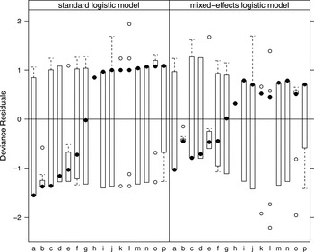
Deviance residuals for a standard logistic model (left) and a logistic mixed model (right) for individuals contributing at least 10 utterances. Each box plot should be centered around 0 (highlighted by the horizontal line).

In keeping with our goal to promote a bridge from sociolinguistic practice to “general statistical practice,” we will use standard statistical terminology. We use predictor as a term covering both numerical predictors (or covariates) and factorial predictors, and we refer to the values of a factorial predictor as its levels. In sociolinguistic practice, a factorial predictor would usually be referred to as a “factor group” or “factor.” In what follows, we represent factor names in boldface and put the levels of a factor in italics.

In our analyses, the external factors are represented by the following predictors: Sex (a factor with levels male and female), Education (a factor with levels low and high), and Age or AgeGroup. AgeGroup is a factor predictor with levels 20–30, 31–50, 51–70, and 70 + , whereas Age is a numeric predictor with the age in years of the individual, for example, 21, 26, 35, 39, 53, 62. We will compare results for age when treated as a numeric rather than factor predictor.

Internal factors

Perhaps the most widely attested linguistic constraint on was/were variation is the effect of polarity, the contrast between affirmative and negative (e.g., Anderwald, Reference Anderwald2002; Britain, Reference Britain2002; Britain & Sudbury, Reference Britain, Sudbury, Jones and Esch1999; Hazen, Reference Hazen1996; Schilling-Estes & Wolfram, Reference Schilling-Estes and Wolfram1994). This effect is present across most varieties, but differs in nature from one variety to the next. The pattern can be explained as a realignment of the past tense morphological forms was and were toward a contrast between negative and affirmative contexts. The most widespread version of this effect is the case where weren't occurs more often in negatives and was occurs more often in affirmatives. This was the pattern found in the earlier analysis of York (Tagliamonte, Reference Tagliamonte1998:180), as in (2).

1. (2) There weren't always bulls. Sometimes there was a few pigs, a few sheep … (YRK/002)

The same pattern is attested in some North American dialects in the United States, for example, North Carolina (Schilling-Estes & Wolfram, Reference Schilling-Estes and Wolfram1994), and across England, including the southwest (Reading) (Cheshire, Edwards, & Whittle, Reference Cheshire, Edwards and Whittle1995), the Fens in the southeast (Britain & Sudbury, 2002), and elsewhere in Britain (Anderwald, Reference Anderwald2002).

The second pattern is when the contrast goes in the opposite direction: nonstandard was occurs more often with negatives, that is, wasn't, and the standard form weren't occurs with affirmatives. This pattern is found in other northern Englishes, such as Northern England (Maryport), southwest Scotland (Cumnock), and Northern Ireland (Portavogie and Cullybackey) (Tagliamonte, Reference Tagliamonte, Fillpula, Klemola and Paulasto2009; Tagliamonte & Smith, Reference Tagliamonte, Smith and Poplack2000:160–161), as in (3).

1. (3)

   1. a. There wasn't any fancy puddings nor no fancy cake nor biscuits. (CMK/-)

   2. b. There were a whole lot of them. (CMK/-)

This pattern is reported in North America for varieties such as African Nova Scotian English (Tagliamonte & Smith, Reference Tagliamonte, Smith and Poplack2000).

A third pattern is also attested. This is where the was variant occurs regardless of polarity (i.e., no polarity effect). This is the pattern reported for New Zealand English, apparently across the 18th and 19th centuries (Hay & Schreier, Reference Hay and Schreier2004:p.228) and (Chambers, Reference Chambers and Kortmann2004:131), as exemplified in (4).

1. (4) No, there wasn't too many cars. There was some, but there wasn't a great many. (WHL/S)

Thus, remorphologization, a common process whereby syntactic phenomena develop morphological contrasts (Joseph & Janda, Reference Joseph, Janda, Hammond and Noonan1986, Reference Joseph and Janda2003) often appears to be an underlying explanation for was/were variation in existentials (see Schilling-Estes & Wolfram, Reference Schilling-Estes and Wolfram1994).

Polarity is coded as a factor named Polarity with as levels affirmative and negative.

Another prominent constraint on this variable relates to the proximity of the verb to its referent or to a plural element (Britain, Reference Britain2002; Hay & Schreier, Reference Hay and Schreier2004; Tagliamonte, Reference Tagliamonte1998). These effects have been subsumed under various labels, including “number shift,” “attraction,” “confusion of proximity” among others. However, they may be explained by different underlying phenomena. One hypothesis is that the agreement relationship between verb and referent becomes compromised when they are distant from each other. This distance is hypothesized to hamper agreement, either as a barrier to direct case assignment (e.g., Henry, Reference Henry1995) or for more general processing reasons (Bock & Kroch, Reference Bock, Kroch, Carlson and Tannenhaus1988). Thus, a crucial consideration is the nature of this underlying relationship. Another hypothesis predicts that the form of the verb will be influenced by a close plural element. Depending on the underlying hypothesis, this predictor must be categorized quite differently. The examples in (5a–5l) will serve to illustrate this.

1. (5)

   1. a. There were badgers in there. (YRK/087)

   2. b. There was [black] clouds. (YRK/078)

   3. c. There were [two] pubs. (YRK/012)

   4. d. There were [the] eggs. (YRK/031)

   5. e. There was [no] treats for them. (YRK/042)

   6. f. There was [some funny] people. (YRK/048)

   7. g. There was [all little] houses in there. (YRK/011)

   8. h. There was [lots of] cinemas. (YRK/16)

   9. i. There was [always] two films on. (YRK/003)

   10. j. There was [four of these] houses . . . (YRK/048)

   11. k. There was [about 12 different] groups . . . (YRK/077)

   12. l. There was [still quite strong] winds in this part. (YRK/078)

   13. m. There was [like purple and green and yellow] bruises. (YRK/049)

For proximity, we have coded the following predictors. First, Proximate1 assesses the number of words intervening between verb and plural element. For example, in (5c) the verb and the first plural element, two, are adjacent, whereas in (5k), there is one word intervening, the adverb about intervenes between was and 12. As the counts of the numbers of intervening words vary substantially (from 1 for 6 intervening words to 198 for 1 intervening word), we also considered a binary factor Proximate1.adj with as levels adjacent (171 observations) and nonadjacent (318 observations), contrasting all cases of adjacent verb to plural element sequences versus nonadjacent ones.

Proximate2 assesses the number of words intervening, but in this configuration, it is the relationship between verb and referent that is relevant. For example, (5h) has two words, whereas (5m) has six words intervening. Proximate1 and Proximate2 distinguish the position of the referent noun phrase (NP) versus a pluralizing element by number of words. As the counts for the different distances vary substantially (from 1 for distances 7 and 8, to 130 for distance 1), we also introduced a factor, Adjacency, that distinguishes between adjacent instances (94 observations) and nonadjacent instances (395 observations), contrasting cases where the verb is adjacent to its referent, (5a, 5b), versus all possible nonadjacent contexts (5c–5l). As we shall see, assessing which of these best accounts for the variation in the data is a key to understanding the phenomenon.

Finally, we configure a predictor to test for the different types of determiner phrases (DP) in which the plural referent is contained, labeled as DP Constituency in the data file. This predictor tests for whether the internal structure of the DP has an effect on the realization of the verb. For example, Milsark (Reference Milsark1977) proposed that strong determiners (i.e., definite articles) that undergo quantifier raising and adjoin to IP (Inflection phrase) permit the verb to get agreement, that is, were whereas weak determiners (i.e., numeric quantifiers, partitive constructions) do not. Although this particular hypothesis was not borne out in the earlier analysis of this feature in York, some other divide within the range of different DP types may remain to be discovered. Thus, we differentiated the following configurations: a bare plural NP (5a); those with a single modifying adjective, quantifier, partitive construction, or combinations thereof (5b–i); no negation (5d); and contexts with adverbs (5h). In this categorization of the data, the number of observations for the different factor levels ranges from 4 (for quantifiers functioning as pronouns), such as There weren't many, to 100 for partitive constructions (5g), for example, There was lots of cinemas. Footnote ³

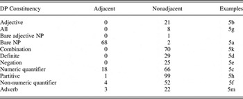
The utterance There was these two other lads was coded as follows: Proximate1 = 0; Proximate2 = 3, Prox1.adj = adjacent; Adjacency = nonadjacent; DP Constituency = definite. The different ways of encoding proximity give rise to a set of highly collinear (nonorthogonal) predictors. Furthermore, neither Proximate1 nor Proximate2 and DP Constituency are fully independent. A large majority (68 of 94) of the observations labeled as adjacent for the factor Adjacency are bare NP (see Table 1). Such interdependencies between predictors are a common phenomenon in sociolinguistic datasets because competing hypotheses are inevitably codependent. We will discuss what options there are to explore such codependent predictors from a statistical perspective.

Table 1.

Contingency table for the predictors DP Constituency and Adjacency

A generalized linear model

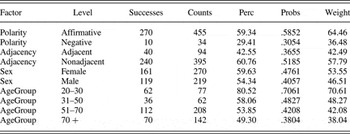
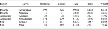
Table 2 presents the results of a variable rule analysis. It is a standard generalized linear model with four predictors: Polarity, Adjacency, Sex, and Age. Adjacency taps into the proximity complex through a binary factorial predictor with as levels adjacent versus nonadjacent, as previously discussed. AgeGroup is configured with four levels: 20–30, 31–50, 51–70, and 70+. The response variable is the binary choice between was and were. The model seeks to predict which variant is used and considers was as a “success” and were as a “failure.” In other words, percentages and probabilities are calculated from the perspective of was, and the model evaluates how often was was used compared to all instances of was and were jointly. We consider a model with main effects only, excluding interactions. In statistics, such a model is referred to as a simple main effects model.

Table 2.

Variable rule analysis, sum coding, all individuals N = 489

Note: Counts are the total number of observations.

Table 2 provides the following information: the predictors considered in the analysis (Factors), their levels (Levels), the number of tokens (Counts), the number of cases with was (Successes), the percentage of such cases (Perc), the corresponding probabilities as estimated by the model (Probs), and the factor weights (Weight). This kind of output is familiar for variable rule analyses. Now, let us consider the results from a general statistical perspective.

The results in Table 2 are based on a series of decisions that jointly define a very specific instantiation of the generalized linear model. A key distinction that is crucial to understanding the reportage in Table 2 is that between unordered and ordered factors. Unordered factors are factors with factor levels that cannot be ordered along a scale of magnitude. Polarity, Adjacency, and Sex are unordered factors. By contrast, Age is an ordered factor as its levels, 20–30, 31–50, 51–70, and 70+ are on a scale from small (young) to large (old).

For unordered factors, the model uses what is known as sum coding. As a consequence, the factor weights (in the column Weight in Table 2) are differences from the grand mean, repositioned around 50%. For ordered factors, variable rule analysis implements polynomial contrasts. Polynomial contrasts are a good choice when the (ordered) predictor levels are equally spaced and have equal numbers of observations. The weights in Table 2 show decreasing probabilities for was with age.

Tables such as Table 2 do not report the coefficients of the underlying generalized linear model, which are on the logit (log odds) scale. This tradition makes a variable rule analysis stand out from the kind of statistical models generally reported in social science or science that may discourage cross-fertilization of knowledge across fields.Footnote ⁵

What information does Table 2 reveal? First, the predictor Polarity, which has two levels, affirmative and negative, receives a weight greater than 50 for affirmative and a weight smaller than 50 for the level negative. This indicates that according to the model the use of was is more likely for affirmative polarity and less likely for negative polarity. This prediction of the model fits well with the observed counts of successes (uses of was) given the total numbers of observations. For affirmative polarity, 270 of 455 (59.3%) observations have was. For negative polarity, only 10 of 34 (29%) of the observations support was. The Probs column lists the proportions predicted by the model given the factor weights it estimated. It is easy to see that the predicted proportions are quite similar to the observed percentages. For the predictor Adjacency, the second unordered predictor in the model, the likelihood of was is slightly greater for nonadjacent contexts and slightly smaller in adjacent contexts. For the predictor Sex, the factor weights are both close to 50. As we will observe, this predictor does not reach significance. Finally, for the ordered factor AgeGroup, we see that as we move down the ordered predictor levels, from the youngest to the oldest group, the factor weights (and the observed percentages and predicted proportions) of was decrease.

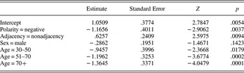
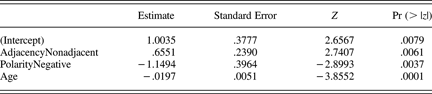
Table 3 presents the results of an analysis using the same statistical tool, the generalized linear model for binary response variables, but now we apply it in a slightly different way. First, instead of examining the effects of predictors on the percentage scale, we consider effects on the log odds scale. On the percentage scale, the 50% mark is the pivotal value; with values greater than 50% indicating a trend in favor of the use of was, and values below 50% indicating a trend against was and in favor of its counterpart were. On the log odds scale, the value of 0 takes over this pivotal role. Positive values now indicate support for was and negative values support for were. Second, instead of using sum coding, we now make use of treatment coding. With treatment coding, one predictor level is selected as the baseline, the so-called reference level. R, when not explicitly instructed otherwise, will select as reference level that predictor level that is the initial one in the alphabetically sorted list of factor levels. For Polarity, the reference level is affirmative, as “affirmative” precedes “negative” in the alphabet. For Adjacency, the reference level is adjacent, and for Sex, it is f(emale). The reference level for AgeGroup is 20–30. Given a reference level, treatment coding instructs the generalized linear model to estimate the differences between the other predictor levels of a given predictor and that predictor's reference level. For Polarity, it will estimate the difference between the mean log odds for negative observations and the mean log odds for the affirmative observations. For Sex, it will calculate the difference between the mean for the men and the mean for the women.

Table 3.

Generalized linear model with only main effects, using treating coding, all individuals N = 489

Which kind of dummy coding is selected is to some extent a matter of personal preference. A first advantage of treatment coding is the coefficients it estimates are well interpretable for unbalanced datasets. For unbalanced designs, dummy coding with sum coding has as a consequence that the interpretation of the coefficients as differences from the group mean is only approximately correct. As a result, the factor weights as listed in Table 2, which are derived from these coefficients, are also approximations. A second advantage of treatment coding is that the coefficients remain transparent when interactions with other factors and with covariates are included in the model specification. We will return to interactions.

The widely varying tokens (number of observations) for the different cells defined by Adjacency, Polarity, and AgeGroup make treatment coding a natural choice for our data. For instance, there are 77 observations for the youngest age group and 62, 208, and 142 for the subsequent age groups. For such an unbalanced dataset, the coefficients of the model are much easier to interpret than are the coefficients obtained with sum coding and with polynomial contrasts for ordered factors (see, e.g., Venables & Ripley, Reference Venables and Ripley2002).

How do we interpret tables such as Table 3? The first row of this table lists the intercept, which represents the reference levels of all factorial predictors in the model simultaneously. In other words, the estimate for the intercept is the mean log odds for the youngest age group (20–30), affirmative polarity, adjacent adjacency, and women. This estimate is positive, indicating that for this combination of predictor levels, was is used more often than were is. The second column presents the standard error associated with this estimate. The standard error is a measure of the uncertainty about the estimate. The larger this uncertainty, the less confidence should be placed in the estimate. The third column presents the Z score, obtained by dividing the estimate by its standard error. This score follows a normal distribution, allowing us to calculate the probability (listed in the fourth column) of observing a more extreme value for the coefficient. Formally, this test asks whether the intercept is significantly different from 0, that is, a 50-50 random use of the two forms. Because for the intercept this probability is small, we can conclude that in all likelihood young women use was significantly more often than chance in affirmative adjacent contexts.

The next row in Table 3 shows that observations with negative polarity have a mean log odds that is −1.17 below that of the intercept. The standard error and its associated Z value show that this difference reaches significance, p = .0037. The group mean that we can calculate from this, 1.0509–1.1656 = −.1147, is calibrated for the young age group, for women, and for adjacent adjacency. When we only change polarity do we get the group mean for negative polarity, youngsters, adjacent adjacency, and women. The second row of the table tells us that the difference between these two group means is significant.

In the next line, only Adjacency changes from adjacent to nonadjacent, so we get young + women + positive + nonadjacent. This illustrates that young women in affirmative polarity use was less often in nonadjacent constructions than in adjacent constructions. This contrast is also significant. The next predictor, Sex, comes with a contrast suggesting that men use was less frequently than women do. However, the large standard error and the low Z value suggest that this small difference is not significant.

Finally, the effect of AgeGroup, a predictor with four levels, appears in the table with three contrasts. There are three predictor levels other than the reference level (the youngest age group), and each of these factor levels is contrasted with the reference level, producing three differences between group means. As the age group increases from 31–50 to 70 + , the magnitude of the estimated contrast increases. From the last column, where the p values are listed, we can observe that each of these three age groups uses was significantly less often than the youngest age group does.

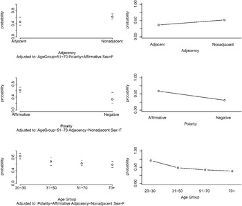
Variable rule analysis with sum coding and our reanalysis using treatment coding make exactly the same predictions, even though these predictions are arrived at in slightly different ways. Figure 2 illustrates this graphically. The left panels present the partial effects of the predictors Adjacency, Polarity, and AgeGroup in the model using treatment coding. The partial effect of a predictor is the effect of that predictor when all other predictors in the model are held constant, where possible at a typical value. For factorial predictors, it is useful to make the reference level the one that comprises the majority of observations. In this way, graphical representations of the data will represent the effects calibrated for the largest possible number of data points (which, with many cells, might be a small minority of all data points.) For numerical covariates, it makes sense to choose the median of that covariate as a typical value.

Figure 2.

Effects of the predictors for a variable rule analysis with sum coding (right), and partial effects of the same predictors in a logistic model with treatment coding (left).

The upper left panel shows the partial effect of adjacency for women in the 51–70 age group, for affirmative polarity. This plot was obtained using the plot facilities for logistic regression models in the Design package of Harrell (Reference Harrell2001), which also adds confidence intervals around the group means. Now consider the lower left panel, which presents the partial effect for AgeGroup. The likelihood of was decreases as age increases. The pattern as shown in this panel is calibrated for affirmative polarity, nonadjacency, and women. For adjacent constructions, we know from the top left panel that the likelihood of was decreases. Hence, to make the bottom left panel precise for adjacent constructions, all four points have to be shifted down according to the amount of contrast between the adjacent and nonadjacent groups in the top left panel.Footnote ⁶ This illustrates what it is to plot a partial effect. The effect is calibrated for specific values of all other predictors in the model. If the value of one of the other predictors changes, the points for the predictor under consideration must be recalibrated as well.

The right panels of Figure 2 present the partial effects for the variable rule model. There are no adjustments listed underneath each panel. This is because in this model all effects are positioned around the grand mean. In the upper right panel, the group means for the two levels of Adjacency show the same difference as in the upper left panel, but they are positioned differently. The group means in the left panel represent actual cells in the design, namely, adjacent and nonadjacent adjacency for women in the 51–70 AgeGroup under affirmative polarity. Because the group means in the upper right panel are calibrated with respect to the grand mean, they do not represent any of the cells in the design. All the other differences between the levels of other factors are averaged out. In other words, the right panels summarize the general trends, the left panels present the same trends but position them specifically anchored with respect to specific cells in the design.Footnote ⁷

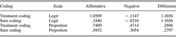
Irrespective of which kind of dummy coding is used, underlying contrasts are estimated on the logit scale. Because the transformation from logits to proportions is nonlinear, the magnitude of a contrast on the proportions scale will vary between sum coding and treatment coding. This is illustrated in Table 4 for the case of the youngest age group producing adjacent sentences, comparing the effect of Polarity on the logit and back-transformed proportions scale (as in a Goldvarb analysis). The difference here is small, but depending on the data, it can be quite substantial. This nonlinearity also affects the confidence intervals for the group means, which on the logit scale are symmetrical around the mean, but, as can be seen in Figure 2 for negative polarity, can become noticeably asymmetrical on the proportions scale.

Table 4.

Contrasts on the logit scale

Notes: Contrasts on the logit scale are identical for sum and treatment coding, but after back-transforming to proportions, differences based on centered factor levels (sum coding) are larger. For treatment coding, the contrast in polarity is that for the youngest age group (20–30) and adjacent sentences.

The two coding systems have both advantages and disadvantages. For balanced datasets, sum coding and polynomial contrasts for ordered factors make it possible to present effects as adjustments from a grand mean, which fits well with the formulation of variable rules in Cedergren and Sankoff (1974), for instance. Unfortunately, for unbalanced datasets, the mathematical interpretation of the coefficients is less straightforward, although for actual practice, the differences are probably benign.

The advantage of treatment coding is that coefficients are well interpretable also for unbalanced designs, as are often encountered when studying language. Furthermore, coefficients remain transparent when interactions and covariates are allowed into the model. The present dataset, as with most sociolinguistic datasets, is in many ways highly unbalanced. As we shall see, inclusion of both covariates and interactions in the model leads to improved prediction accuracy. Thus, we will use treatment coding for the remainder of this study.

Interactions and covariates

The model introduced in the preceding section (Tables 1 and 2) uses a factorial predictor, AgeGroup, to represent the age of the individuals. The predictor is divided into categories known as factors or levels. One disadvantage of this method is a potential loss of power, in other words, the likelihood of detecting an effect that is actually present in the data decreases (see, e.g., Baayen, Reference Baayen2010, and references cited there). Another disadvantage is that the cutoff points for the different age groups may be somewhat arbitrary, however carefully they may have been devised.

In Figure 2, the bottom panels indicate that the effect of AgeGroup is nonlinear. The difference in the probabilities for the youngest age groups is larger than the corresponding difference for the oldest two age groups. This kind of trend, with an effect that becomes smaller with each step, is a negative decelerating trend. When replacing AgeGroup by Age, we should not expect to be able to model the negative decelerating effect of Age simply with a straight line

(1)

(In this equation, β₀ is the point on the vertical axis at which the line intersects the vertical axis, and β₁ is the slope of the line.) Instead of the formula for a straight line, what we need is a mathematical formula that can faithfully represent the observed curvature. In the present case, the curve looks like it might be part of a parabola. (In nature, the trajectory of a bouncing ball between two points where it touches the ground is part of a parabola.) Mathematically, a parabola is described by a quadratic polynomial, which adds a second parameter and a quadratic term to the equation of a straight line, as follows:

(2)

The coefficient β₂ is referred to as the quadratic coefficient as opposed to β₁, the linear coefficient.

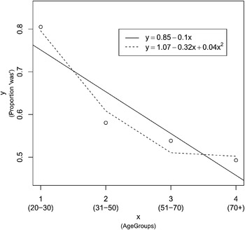
Figure 3 illustrates the difference between a linear (solid line) and a quadratic fit (dotted line) for the trend across the four age groups visible in the lower panels of Figure 2. When modeling the effect of AgeGroup as a factor, no constraints are placed a priori on what kind of pattern the contrasts should follow. Some might be larger than the reference level, others smaller. When moving from an ordered factor (with imposed levels) to the underlying covariate, we may discover that the linear model is too restrictive. This can be seen in Figure 3, where the values on the horizontal axis range from 1 to 4, and the values on the vertical axis represent the proportions of was responses. The solid line represents a linear fit to the data, using for simplicity a standard Gaussian model. The dashed line represents a model with a quadratic polynomial. The amount of variance explained increases from .83 to .97. The addition of a second parameter allows us to model the observed trend more precisely.

Figure 3.

Linear and quadratic fits to a nonlinear trend (proportion was as a function of age group, compare the lower panels of Figure 2.

Let us now test the difference between using a linear model for the factor AgeGroup and a quadratic model for the covariate Age (expressed in years), using logistic regression. Before we do so, recall that thus far, our statistical models have examined the data with only main effects. Such simple main effects models are correct only if each predictor has an effect that is independent of the effects of the other predictors. For any given dataset, this assumption may or may not be appropriate. It turns out that the effect of Age differs for affirmative and negative polarity, and that a simple main effects model is too simple.

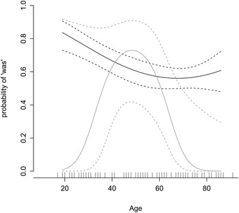
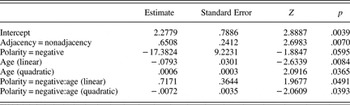
Table 5 shows the coefficients of a model that includes linear and quadratic terms for Age, and that allows both these terms to interact with Polarity. (In this model, the predictor Sex is not included, because the preceding analyses indicated it does not reach significance.) The easiest way to understand what the model does is to inspect the visual representation of the interaction of Age by Polarity presented in Figure 4. The black lines represent the effect of Age for affirmative polarity and its 95% confidence intervals. As Age increases, the probability of was decreases. The gray lines represent the effect of Age for negative polarity. Because there are only 34 observations with negative polarity, compared to 455 observations with affirmative polarity, the confidence intervals are much wider, and no definite conclusions should be drawn from the analysis. However, the trend that we see in Figure 4 is that in utterances with negative polarity, was is favored by individuals around 50 years of age and disfavored by the youngest and oldest individuals. This is a classic age-grading pattern and it shows us that affirmative and negative contexts reflect socially independent phenomena in this speech community.

Figure 4.

Partial effect of Age for sentences with affirmative (black) and negative (gray) polarity, with 95% confidence intervals.

Table 5.

Estimated coefficients, standard errors, Z and p values for a generalized linear model with an polynomial (degree 2) for Age in interaction with Polarity, using treatment coding N = 489

Now consider the interpretation of the coefficients listed in Table 5. The intercept represents adjacent affirmative construction for individuals with age 0. There are, of course, no such individuals in our sample. All data points are located far to the right of the vertical axis. Nevertheless, mathematically, the regression curves will intersect the vertical axis at some point, and for the adjacent affirmative constructions, this point is 2.28. The positive and significant contrast coefficient (.65, p = .007) for Adjacency = nonadjacent indicates that the probability of was increases for nonadjacent constructions compared to adjacent constructions (for age 0). The third row of the table indicates that for negative polarity, the likelihood of was decreases substantially (−17.4, p = .06), again for age 0. (There are few data points here, so the standard error is large and the effect does not reach full significance.)Footnote ⁸

The last two rows of Table 5 provide treatment contrasts that change the black curve in Figure 4 into the gray curve in Figure 4. On the logit scale, the black curve is given by

(3)

and the gray curve for negative polarity is given by

(4)

Note that all three coefficients in (3) are adjusted for negative polarity: the intercept, the linear coefficient of Age, and the quadratic coefficient of Age. When the parabola defined by (4) on the logit scale is transformed to the probability scale, the gray curve of Figure 4 results.

The model summarized in Table 5 invests no less than five parameters for the modeling of Polarity and Age. Does this investment pay off by leading to a model that fits the data better? This question can be answered in two ways. First, we can compare the present model with a much simpler model with simple main effects for Adjacency, Polarity, and Age. This model requires only four parameters: an intercept, two contrast coefficients, and one slope (see Table 6).

Table 6.

A main effects model with Adjacency, Polarity, and Age as predictors

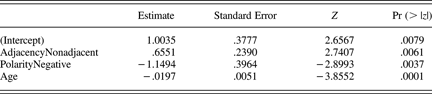
However, upon inspection it turns out that the residual deviance for this simpler model, 631.28, exceeds the residual deviance of the complex model, 616.76, by 14.52. This reduction in deviance follows a chi-squared distribution with as degrees of freedom the difference in the number of parameters, 3. The associated p value, .002, obtained with this analysis of deviance indicates that the more complex model provides a significantly better goodness of fit. (For the example code in R, the reader is referred to the Appendix.)

Second, we can also compare the model of Table 5 with the original model with Adjacency,Polarity, Sex, and AgeGroup as predictors. That model also invested seven coefficients (see Table 3). In this case, an analysis of deviance cannot be applied because both models invest the same number of parameters, and also because the models to be compared are not nested. For situations like this, it is often useful to use the index of concordance C. This index is a generalization of the area under the receiver-operating characteristic curve in signal detection theory (for examples, see, e.g., Baayen, Reference Baayen2008; Harrell, Reference Harrell2001). It measures how well the model discriminates between the was and were responses. When C = .5, classification performance is at a chance, and values of C ≥ .8 indicate a good performance. For the simple main effects model with Adjacency, Polarity, Sex, and AgeGroup,C = .659. For the model of Table 5, there a slight improvement to C =.66. For both models, however, the low value of C is a signal that the fit of the model to the data is not particularly good, which means that we have not yet arrived at a satisfying model to help interpret and explain the variation. One possibility is that there is simply a lot of noise in the data, and that this is the best we can do. Alternatively, it is possible that we are neglecting to enlist an alternative, and accessible, statistical tool, and that a much better fit is actually within reach.

Generalized linear mixed-effects modeling

In our analyses so far, we have not considered the individuals in the sample. These individuals will undoubtedly differ in their own personal preferences for was versus were. The question is, to what extent? Because the individuals contributing to the current dataset are a small sample (83 individuals) of the locally born population of the city of York, Individual is a random-effect factor. Random-effect factors differ from fixed-effect factors such as Adjacency or AgeGroup in that the latter have a fixed and usually small number of factor levels that are repeatable. Repeatable in this sense contrasts Adjacency, which would have the very same factor levels in a replication study, namely adjacent versus nonadjacent, with Individual, which in a new random sample would likely contain an entirely different set of individuals.

Variable rule analysis can only model Individual as a fixed effect in the existing dataset. This has several disadvantages compared to mixed-effects models. First, it is not possible to generalize to the population that the dataset is meant to represent. The model pertains only to the individuals who happened to be included in the sample.

Second, the estimated effects for the individual do not benefit from shrinkage. An individual evidencing an extreme preference for were in one random sample of elicited utterances is likely to show a reduced preference for were in a second random sample. This is an instance of the general phenomenon of regression toward the mean (often illustrated with the example that sons of very tall fathers tend to be less tall than their fathers are). Shrinkage anticipates regression toward the mean, providing estimates for the individual differences that are more realistic, more precise, and hence afford enhanced prediction for replication studies with the same individuals.

Third, mixed models offer a flexible way of taking into account not only that individuals may have different preferences, but also that their sensitivity to, for instance, Polarity, may differ significantly. We will return to this point in more detail.

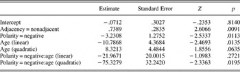
As a first mixed-effects model for our data, we begin with the model of Table 5 and simply add in Individual as a random-effect factor, allowing the intercept to be adjusted for each individual separately. This model with by-individual random intercepts assumes that the effects of Adjacency and Polarity are the same across all individuals, but allows individuals to have different baseline preferences for was versus were. Table 7 presents the coefficients for Adjacency, Polarity, and Age and their associated statistics.

Table 7.

Coefficients of a generalized linear mixed-effects model with random intercepts for individuals (SD 1.3345), using treatment coding and an orthogonal polynomial of degree 2 for Age

What is new in the mixed model is an additional parameter that specifies how variable the individuals are with respect to their baseline preferences. This parameter, a standard deviation, was estimated at 1.33. This standard deviation squared is the variance of the individual baseline preferences.

Does the addition of this new parameter lead to an improved goodness of fit? This question is answered by comparing the original model (refitted with an orthogonal polynomial) with its mixed counterpart, using an analysis of deviance test. As the deviance is substantially reduced, from 616.76 to 565.02, it is not surprising that the mixed model provides a significantly better fit (X ₍₁₎Footnote ² = 51.742, p < .0001). The index of concordance C increases substantially to.87, well above .8, providing statistical validation of a good fit. Finally, we have achieved an acceptable statistical model.

It is an empirical question whether by-individual random intercepts (or any further more complex random-effects structure) are justified for a given dataset. When only a single observation is available per individual, it is not possible to include the individual as a random-effect factor. In that case, a generalized linear model suffices. However, for many practical situations, collecting only a single instance from each individual is prohibitively costly. Although variationist practice sometimes advocates restricting the number tokens per type for each individual (Wolfram, Reference Wolfram and Preston1993), from a technical perspective, even a small number of by-individual replications causes problems for the classical statistical model. An advantage of the mixed-effects modeling framework is that it allows the researcher to sample as many tokens from a given individual as is feasible, thereby increasing statistical power. This also opens up additional possibilities to study how individuals differ systematically over and above the differences between the groups to which they belong. This may turn out to be useful for understanding the variation at the speech community level.

Returning to our data, it is worth noting that to this point we have assumed that the only difference between the individuals is their baseline preference for was versus were. However, there is some indication of significant variability in the sensitivity of the individuals to Polarity, which emerged in Figure 4 as linked to individuals' age, and which in our current mixed-effects model is accounted for by an interaction of Polarity by Age. When we relax the assumption that the effect of polarity is exactly the same for all individuals by allowing by-individual random contrasts for Polarity into the model specification, we obtain a model with a significantly improved goodness of fit, according to a likelihood ratio test (X ²_(x) = 7.91, p = .0191). Nevertheless, we are skating on thin ice. More than one-half of the individuals do not have a single negative token. The remaining individuals typically provide only a single example, with a maximum of four. Unfortunately, the paucity of data does not warrant further exploration of individual differences for Polarity.

Random forests

Consequently, we turn to a relatively new tool: random forests. Random forests were developed by Breiman (Reference Breiman2001), building on earlier work on classification and regression trees (Breiman, Friedman, Olshen & Stone, Reference Breiman, Friedman, Olshen and Stone1984). In what follows, we make use of the implementation of random forests available in the party package in R (Strobl, Boulesteix, Kneib, Augustin, & Zeileis, Reference Strobl, Boulesteix, Kneib, Augustin and Zeileis2008; Strobl, Boulesteix, Zeileis, & Hothorn, Reference Strobl, Boulesteix, Zeileis and Hothorn2007; Hothorn, Buehlmann, Dudoit, Molinaro, & Van Der Laan, Reference Hothorn, Buehlmann, Dudoit, Molinaro and Van Der Laan2006), which implements forests of conditional inference trees (Hothorn, Hornik, & Zeileis, Reference Hothorn, Hornik and Zeileis2006). Like logistic models, random forests seek to predict, given a set of predictors, which of the alternatives was or were is most probable. However, these statistical techniques achieve the same goal quite differently. Logistic models predict the choice between was and were based on a mathematical equation such as (3), which specifies for each predictor how it affects this choice. Thanks to various simplifying assumptions, the mathematics of these models makes it possible to estimate the parameters quickly and efficiently.

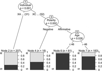
Random forests, in contrast, work through the data and, by trial and error, establish whether a variable is a useful predictor. The basic algorithm used by the random forests constructs conditional inference trees. A conditional inference tree provides estimates of the likelihood of the value of the response variable (was/were) based on a series of binary questions about the values of predictor variables. For instance, for Adjacency, it considers whether splitting the data into adjacent and nonadjacent utterances goes hand in hand with the creation of one set of data points where was is used more often and another set where were is used more often. The algorithm works through all predictors, splitting (partitioning) the data into subsets where justified, and then recursively considers each of the subsets, until further splitting is not justified. In this way, the algorithm partitions the input space into subsets that are increasingly homogeneous with respect to the levels of the response variable.

The result of this recursive binary splitting of the data is a conditional inference tree. At any step of the recursive process of building such a tree, for each predictor, a test of independence of that predictor and the response is carried out. If the test indicates independence, then that predictor is useless for predicting the use of was or were. If the null hypothesis of independence is rejected, the predictor is apparently useful. If there are no useful predictors, the algorithm stops. If there is more than one useful predictor, the predictor with the strongest association with the response is selected, the p value of the corresponding test is recorded, and a binary split based on that variable is implemented. Conditional inference trees implement safeguards ensuring that the selection of relevant effects (predictors, variables) is not biased in favor of those with many levels (multiple factors in a factor group), or biased in favor of numeric predictors (e.g., age of the individuals).

Random forests construct a large number of conditional inference trees (the random forest). Each tree in the forest is grown for a subset of the data generated by randomly sampling without replacement (subsampling) from observations and predictors. The metaphor used in statistics is of putting part of the observed data into a bag. The data in the bag is referred to as the in-bag observations. The data points that were not sampled are referred to as the out-of-bag observations. The consequence of this procedure is that for each tree a training set (the in-bag observations) is paired with a test set (the out-of-bag observations). The accuracy of a tree's predictions is evaluated by comparing its predictions for the out-of-bag observations with the actual values observed for the out-of-bag observations.

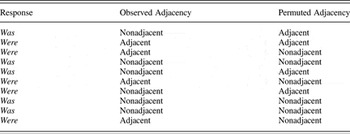
To evaluate how useful a predictor is, a permutation variable importance measure is used. Suppose that a given predictor is associated with the response variable. For example, were (as opposed to was) is associated with adjacency. By randomly permuting the values of the predictor, the association with the response variable is broken. An artificial example illustrating this point is given in Table 8. For the observed adjacencies, all but one nonadjacent utterance is paired with was, and all adjacent utterances are paired with were. When the levels of Adjacency are randomly permuted, this difference between was and were is erased. In this example, after permutation, adjacent utterances occur equally often with both forms, and the same holds for the nonadjacent utterances.

Table 8.

Example of how permuting the levels of a predictor can break its association with the response variable

In random forests, the permuted predictor, together with all the other predictors, is used to predict the response for the out-of-bag observations. If the original, unpermuted predictor was truly associated with the response, that is, if the original predictor is a significant predictor of the response, then a model with the permuted version of the original predictor must be a less accurate classifier. In other words, classification accuracy will decrease substantially if the original, unpermuted predictor was truly associated with the response. The extent to which the model becomes worse is a measure of the importance of a predictor. If the model hardly becomes worse, then a predictor is not relevant. However, if the model's performance decreases dramatically, we know that we have a vital predictor. Breiman (Reference Breiman2001) therefore proposed the difference in prediction accuracy before and after permuting the predictor, averaged over all trees, as a measure for variable importance.

In the present study, we make use of an improvement of this measure, the conditional variable importance measure implemented in the Cforest function of the Party package. Strobl et al. (Reference Strobl, Boulesteix, Kneib, Augustin and Zeileis2008) showed that Breiman's original permutation importance severely overestimates the importance of correlated predictor variables. They proposed a conditional permutation scheme that protects the evaluation of a variable's importance against inflation. For instance, in the present study of was/were variation, Age is a sensible predictor. A variable such as income, which correlates with age (older people tend to have higher incomes), is not a sensible predictor. Without appropriate measures, a random forest would nevertheless assign income a high variable importance, whereas a simple linear model would immediately detect that income is irrelevant once age is incorporated as a predictor. The conditional permutation variable importance implemented in the Cforest function of the Party package correctly reports spurious predictors such as income to have a very low variable importance.

Having outlined how the importance of variables is gauged by random forests, we finally need to introduce how a random forest is used to obtain predictions. After all, we are now dealing not with a single tree, but with a forest of trees. The solution adopted by the random forest technology is to make use of a voting scheme. All the trees in the forest contribute a vote based on what each tree thinks is the most likely response outcome—was or were. The prediction of the tree is the outcome that receives the greatest proportion of the votes.

Random forests provide a useful complement to logistic modeling in three ways. First, because random forests work with samples of the predictors, they are especially well applicable to problems with more variables than observations, that is, “small n large p” problems. This situation is the typical case in sociolinguistic research where many studies are based on a relatively small number of tokens (observations) and a large number of predictors. Second, subsampling combined with conditional permutation variable importance estimation reduces substantially the problem of collinearity (correlated factors) that can severely destabilize regression models (Belsley, Kuh & Welsch, Reference Belsley, Kuh and Welsch1980). Third, empty cells, linear constraints in the predictors, or perfect separation of response classes in particular combinations of predictors may render regression modeling, or the exploration of interactions in a regression model, impossible. Random forests do not have these estimation problems, making them the ideal panacea for the thorniest problems of variation analysis. The added value is that random forests allow the researcher to explore more aspects of the data and by consequence more insights into the explanation for variable processes. (For an excellent introduction to random forests, see Strobl, Malley, & Tutz [Reference Strobl, Malley and Tutz2009].)

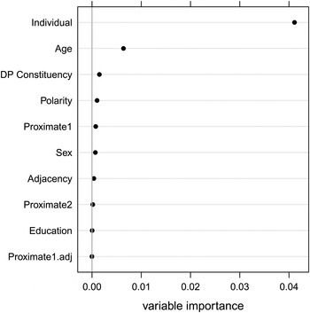
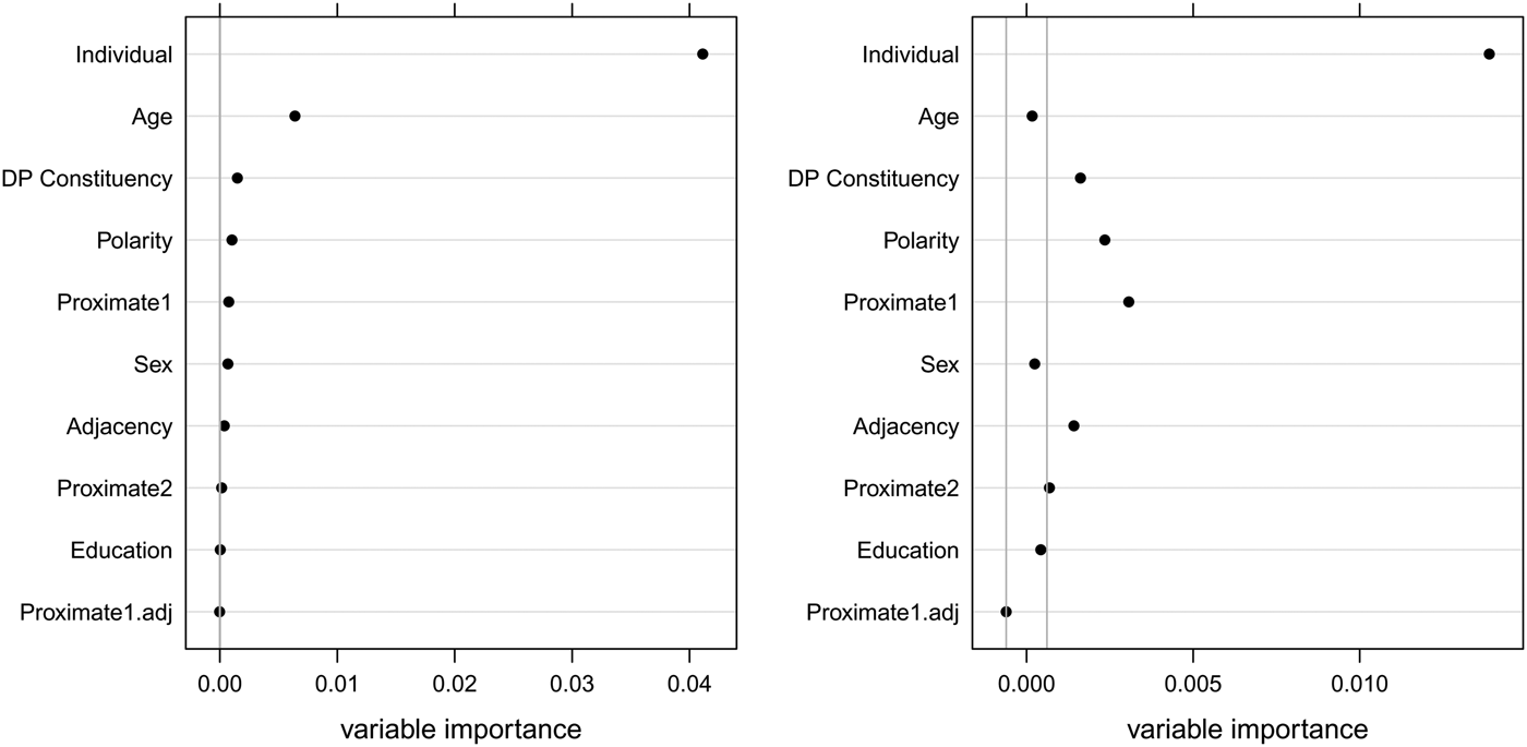
A random forest for our data with just the four predictors—Adjacency, Polarity, Age, and Individual—comes with an index of concordance for this model, C = .88 that already presents a slight improvement on the value (.87) obtained for the corresponding mixed model summarized in Table 7. However, the real power of the random forest becomes apparent when we consider other predictors that are available, but that were not included in the analyses with the generalized linear model (Tables 1 and 2) due to covariation with other predictors, highly unequal cell counts, empty cells, and such. Figure 5 presents the variable importance for the predictors Individual (the people in the sample), Age (the actual age of each person), Polarity, DP Constituency (11 levels, including levels such as bare NP, numeric quantifier, partitive, and definite), the individuals' level of Education (high versus low), the Sex of the individual (male versus female), and the four different schemas for categorizing adjacency. Note that within the linear modeling framework (including variable rule analysis), it would be impossible to explore simultaneously these highly correlated measures for Proximity and DP Constituency. The index of concordance for the model with the full set of predictors increases to C = .92.

Figure 5 depicts the relative importance of the predictors, using conditional permutation-based variable importance. The gray vertical line highlights the variable importance of the inconsequential predictors, which is for all practical purposes equal to 0.

What Figure 5 shows is that the individual is by far the most important predictor. Substantial variability tied to the individual is also found in almost any psycholinguistic experiment (see, e.g., Baayen, Reference Baayen2008), where a subject random-effect factor invariably accounts for much of the variance. A key advantage of using mixed-effects models for sociolinguistic studies will be the ability to amass a similar foundation of research. Analysts will be able to document the extent and nature of individual variance for linguistic features at all levels of grammar and across speech communities.

The next most-important predictor is Age, an external predictor also tied to the individual. Some predictivity is detectable for DP Constituency, Polarity, Proximate1, and Sex. None of the other predictors contributes statistically significant effects, as indicated by the vertical gray line.

Before exploring how the predictor variables work together in predicting the choice between was and were, we emphasize again that the predictors considered jointly in this random forest are nonorthogonal and collinear. In particular, Proximate1, Proximate2, Prox1.adj, and Adjacency, though not tapping into precisely the same underlying mechanism, are nonetheless highly collinear phenomena. Moreover, DP Constituency mirrors Proximity to a high degree because certain modifying structures in the DP are more complex and inevitably longer than others are (e.g., quantifier phrase versus bare NP). In a linear model, these predictors should never be considered together (see, e.g., Guy, Reference Guy, Ferrara, Brown, Walters and Baugh1988). Even when considered jointly in a (mixed) linear model, unsolvable computational problems arise, and error messages of various kinds are generated. The random forest, however, is immune to this kind of problem. It will consider all variables in their own right (factorial or numeric) and identify which of these variables is the superior predictor.⁹

Another useful property of the random forest is that it does not suffer from being excessively complex with too many predictors relative to number of observations (i.e., overfitting) and it is not hampered by small or even zero cell counts. For the present set of tests for proximity, Proximate1 and DP Constituency are among the top three of the internal predictors in the analysis, together with Sex. These are among the most fine-grained predictors, one measuring distance in words to the plural referent and the other measuring the nature of the composition of the DP. Their relative importance reveals that the nature of the DP is a more germane predictor.

Thus, it becomes critical to understand the difference between these two predictors. Proximate1 measures the proximity to a plural element and was is more likely in these contexts. DP Constituency identifies the different types of determiner phrases in the data. One of the most prominent types is partitive constructions (and combinations thereof), which are more likely to occur with was as well. Indeed, previous research has suggested a universal hierarchy of DP Constituency. So far, however, the rankings of categories have differed across studies (e.g., Hay & Schreier, 2004; Walker, Reference Walker2007). This may be because the distribution of DP types varies by dataset or it may be due to varying coding strategies, but the fact that it turns up across studies is suggestive, and in most cases, the highest ranked category involves numbers: There was 3 of us; there was about 50 of us. However, such constructions may or may not be grammatically plural despite the evident plural element. The relative ranking of DP Constituency in our analysis suggests that another underlying reason for variant was could be explained by certain NP constructions, in this case, ones that are being reanalyzed as singular, not plural, hence was not were. To fully substantiate this hypothesis, a more detailed semantic-syntactic analysis of DP Constituency is required.¹⁰

In order to clarify how the predictors evaluated by the random forest work together, we now consider the conditional inference tree for the data, grown with all predictors included. The superiority of a random forest (Figure 5) compared to a single conditional inference tree, grown with all predictors and all data points (see Figure 6) is evident from the inferior index of concordance for the single tree, C = .79. Nevertheless, the conditional inference tree highlights the complex interaction characterizing this dataset. Polarity is relevant only for a subset of the individuals, and the effect of Age is further restricted to positive polarity items for that subset of individuals, in congruence with the linear model's evaluation of this interaction (cf. Figure 4).

Figure 5.

Conditional permutation variable importance for the random forest with all predictors. Predictors to the right of the rightmost vertical gray line are significant.

Figure 6.

Conditional inference recursive partitioning tree.

Complex interactions, such as the one observed here, involving Individual, Age, and Polarity, can be difficult or even impossible to capture adequately even with a mixed-effects logistic linear model. In order to capture the differences between the individuals emerging from the conditional inference tree, the random-effects structure of the mixed-effects model would have to be enriched with by-individual random effects for Polarity and Age, as well as individual differences for the interaction of Polarity by Age. We have briefly mentioned that including random contrasts for Polarity improved the fit of the mixed model. But we also observed that there were very few examples of negative polarity in the data, which is why we did not pursue a more complex random-effects structure. The conditional inference tree indicates that a much more complex random-effects structure is required than we anticipated there. However, due to data sparsity, the mixed-effects model that we fitted to the data, with no less than 10 random-effects parameters, was clearly stretched beyond its limits and is not discussed further here. In contrast, the random forest and conditional inference tree offer an ideal tool to be used in tandem with the mixed-effects logistic model to come to a full understanding of the quantitative structure of a dataset and, as a result, an optimal interpretation of the variation. In this case, we are pointed to the fine-grained distinctions among the predictors, particularly, Proximate1 and DP Constituency. Their relative importance points to the predictor that offers the better explanation for was/were variation and to which we should turn to inform our interpretation of the data.

In summary, for naturalistic, unbalanced data with complex interactions, random forests help overcome the limitations of mixed-effects models, although the reader should be warned that this comes at the cost of substantially more computing time. The smart mathematics underlying the mixed model makes it possible to fit a model to the present dataset in a few seconds. By contrast, even with smart computational optimization, the calculation of variable importance, based as it is on extensive permutation schemes, can take many hours to complete.

Restricting the analysis to variable individuals

The final question that we consider here is whether only variable individuals should be included in the analysis. In the present dataset, there are 38 individuals who show no variation in their choice of was versus were. Variationist methodology typically recommends that categorical individuals be removed for the study of variable phenomena (e.g., Guy, Reference Guy, Ferrara, Brown, Walters and Baugh1988:130). However, in practice, particularly with morphosyntactic and discourse-pragmatic features, they are often included on the assumption that internal predictors will be parallel across individuals. The question is whether or not these individuals without variation are a source of noise that should be taken out before the start of the analysis? Would the relative importance of the predictors change if a random forest were fitted to the data after exclusion of the nonvariable individuals?

Table 9 shows a variable rule-style simple main-effects model for the variable individuals only (compare Table 1; C = .622). AgeGroup is not significant (and was therefore removed from the model specification). Instead, Sex now takes over as a significant external predictor. In a mixed-effects model including random intercepts for Individual, the effect of Sex is marginal (p = .0621, two-tailed test), but women favored was. This is the result for Sex reported in the original study of was/were variation in York for a smaller set of individuals (Tagliamonte, Reference Tagliamonte1998:181). When a random forest is grown for this subset of the data, the index of concordance C equals .88, a value that is lower than that for the random forest for all individuals (C = .92), but higher than the value reached by the model for all individuals when its predictions are evaluated for just the subset of data with variable individuals (C = .78). As can be seen in Figure 7, the importance of the variables changes as well. Age is now irrelevant, whereas Polarity and Proximate1 and, to a lesser degree, Adjacency and DP Constituency have gained importance.

Figure 7.

Conditional inference recursive partitioning trees for all individuals (left) and for variable individuals (right).

Table 9.

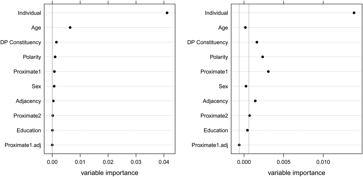
Variable rule analysis, sum coding, variable individuals only N = 357

In the right panel of Figure 7, two vertical gray lines are displayed. These lines have been added by hand to highlight the relative importance of the predictors. Those on the left line or below can be considered superfluous, whereas those on the right are taken to be acceptable.

These changes indicate that the nonvariable individuals are not just random noise. Being a nonvariable individual must be, at least in part, predictable from the other variables. To pursue this possibility, we fitted both a conditional inference tree and a logistic model to the data with as a dependent variable whether the individuals did not show any variability (models not shown). The generalized linear model pointed to a highly significant effect of Age (older individuals are more variable, p < .0001) and possibly effects of Polarity (negative polarity increases variability, p = .0446) and Adjacency (nonadjacency decreases variability, p = .0573). With an index of concordance C = .68, this model did not outperform a conditional inference tree with a single split in age at 60: C = 0.69 (see Table 10).

Table 10.

Deterministic and variable individuals cross-classified by an age cutoff at 60 years, as suggested by a conditional inference tree

This example illustrates the more general methodological point, namely, that the effect of categorical and noncategorical individuals should be brought into the analytical exploratory maneuvers of a variationist analysis (Guy, Reference Guy and Labov1980). Are the categorical individuals random or can they be predicted by other variables? It makes sense to zoom in on what might be going on with variable informants, otherwise valuable information might be swamped by noise. Now that statistical techniques are available that can easily include the individual as part of the analysis, sociolinguists will be able to deepen their understanding of the dialectic between individual and group behavior.