1. Introduction
Taylor’s frozen turbulence hypothesis is widely adopted in spectral analysis using time-series experimental data (Taylor Reference Taylor1938). According to this hypothesis, frequency-domain information can be converted into the wavenumber domain using the relation
 \begin{equation} k=2\pi f/U, \end{equation}
where
 $k$
is the wavenumber,
 $f$
is the frequency and
 $U$
is the local mean velocity at the measurement point. The key assumption of Taylor’s hypothesis is that the convection velocity is identical to the local mean velocity. This assumption allows conversion into the wavenumber domain from a single-point measurement and is the reason the hypothesis has been widely used in turbulence studies. However, it is also well known that the actual convection velocity often differs from the local mean velocity (see Goldschmidt, Young & Ott Reference Goldschmidt, Young and Ott1982). Numerous previous studies have highlighted the limitations of Taylor’s hypothesis and proposed various corrections to address them (e.g. del Álamo and Jiménez Reference del Álamo and Jiménez1982; Zaman and Hussain Reference Zaman and Hussain1982; Choi & Moin Reference Choi and Moin1990; Khoo et al. Reference Khoo, Chew and Teo1990; Mi and Antonia Reference Mi and Antonia1990; Monty & Chong Reference Monty and Chong2009). These correction methods, however, are not widely applied, and there are no established alternatives. As a result, Taylor’s frozen turbulence hypothesis, which assumes the convection velocity to be the local mean velocity, is still commonly used. In this context, a straightforward approach to applying (1.1) more accurately, as noted by many previous studies (e.g. Quadrio and Luchini Reference Quadrio and Luchini1990), is simply to determine the convection velocity
 $U_{\textit{cv}}$
with greater accuracy. To this end, numerous studies – dating back several decades – have focused on the estimation and characterisation of convection velocity.
Taylor’s hypothesis is frequently employed in the spectral analysis of wall-bounded turbulence as well. A key feature of the convection velocity in such flows is that it closely matches the local mean velocity in the outer region, whereas in the near-wall region, it tends to exceed the local mean velocity. This behaviour has been reported in numerous studies. Experimental observations by Krogstad et al. (Reference Krogstad, Kaspersen and Rimestad1998), Österlund et al. (Reference Österlund, Lindgren and Johansson1990), LeHew, Guala & McKeon (Reference LeHew, Guala and McKeon2010), Atkinson, Buchmann & Soria (Reference Atkinson, Buchmann and Soria2015) and Dróżdż et al. (Reference Dróżdż, Niegodajew, Romańczyk and Elsner2015), as well as numerical simulations by Kim & Hussain (Reference Kim and Hussain1993), del Álamo and Jiménez (Reference del Álamo and Jiménez1982), Liu & Gayme (Reference Liu and Gayme2020) and Mehrez, Yamamoto & Tsuji (Reference Mehrez, Yamamoto and Tsuji2023) support this trend. In regions where the convection velocity deviates from the mean velocity, Monty & Chong (Reference Monty and Chong2009) demonstrated that there was good agreement between experimental and direct numerical simulation (DNS) spectra when the appropriately corrected convection velocity was used. This underscores the importance of accurately estimating the convection velocity when applying Taylor’s hypothesis to convert frequency-domain data into the wavenumber domain in wall-bounded flow. However, since even the scaling laws for the mean velocity profile remain under debate in this flow field (e.g. Kim Reference Kim2012), quantitative discussions of the convection velocity – particularly at high Reynolds numbers – are still limited. For the near-wall region, several studies (e.g. del Álamo and Jiménez Reference del Álamo and Jiménez1982; Österlund et al. Reference Österlund, Lindgren and Johansson1990; Kim & Hussain Reference Kim and Hussain1993) have reported that the convection velocity is approximately uniform across wall-normal positions and consistently exceeds the local mean velocity. However, Atkinson et al. (Reference Atkinson, Buchmann and Soria2015) challenged this view, reporting that the convection velocity decreases when approaching the wall and that a uniform convection velocity was not observed in their measurements. These discrepancies highlight that the detailed wall-normal profile and Reynolds-number dependence of the convection velocity in wall-bounded flows are not yet fully understood.
Another important issue concerning the convection velocity in wall-bounded flows is its scale dependence in the near-wall region. Kim & Hussain (Reference Kim and Hussain1993) reported that the convection velocity increases with the scale of turbulent structures near the wall, whereas no such scale dependence is observed farther from the wall. del Álamo and Jiménez (Reference del Álamo and Jiménez1982) found that the convection velocity of small-scale structures (with wavelengths smaller than
 $2h$
, where
 $h$
is channel half-width) is nearly consistent with the local mean velocity, whereas that of larger structures (greater than
 $2h$
) is more closely related to the bulk velocity. Choi & Moin (Reference Choi and Moin1990) and Krogstad et al. (Reference Krogstad, Kaspersen and Rimestad1998) estimated the convection velocity using two-point correlations and reported that it increases with the separation distance between measurement points, further indicating the existence of scale-dependent convection velocity. Most previous studies have reported that this scale dependence is primarily observed in the near-wall region. However, as Atkinson et al. (Reference Atkinson, Buchmann and Soria2015) observed scale-dependent convection velocity through phase-spectral analysis extending from the near-wall region to beyond the boundary-layer thickness, it is possible that such effects are not confined to the vicinity of the wall.
In this context, large-scale motions with streamwise lengths of the order of
 $10R$
to
 $20R$
(where
 $R$
is the pipe radius), which appear in the logarithmic region of mean velocity profile in high-Reynolds-number wall-bounded flows, have come into focus in discussions of convection velocity. These structures, commonly referred to as very large-scale motions (VLSMs), have been revealed through pre-multiplied spectrum (PMS) analysis (e.g. Marusic et al. Reference Marusic, McKeon, Monkewitz, Nagib, Smits and Sreenivasan2010a
; Vallikivi, Ganapathisubramani & Smits Reference Vallikivi, Ganapathisubramani and Smits2015; Ono, Furuichi & Tsuji Reference Ono, Furuichi and Tsuji2025). Since the initial report by Kim & Adrian (Reference Kim and Adrian1999), many studies have focused on these structures, yet their characteristics are still not fully understood (see Marusic, Mathis & Hutchins Reference Marusic, Mathis and Hutchins2010). The VLSMs are typically identified in high-Reynolds-number flows based on spectral analysis employing Taylor’s hypothesis. Such results have been obtained not only through hot-wire anemometry but also through laser Doppler velocimetry (LDV) measurements (Ono et al. Reference Ono, Furuichi and Tsuji2025). It is important to note, however, that the convection velocity of VLSMs has not been clearly identified. Given that much of the discussion on VLSMs relies on spectral analysis, determining their convection velocity is evidently a crucial issue. The large-scale structures discussed by del Álamo and Jiménez (Reference del Álamo and Jiménez1982) are defined as those larger than
 $2h$
, but they are not explicitly referred to as VLSMs, and the Reynolds number in that study is relatively low, which may not have been sufficient for observing VLSMs. Dennis & Nickels (Reference Dennis and Nickels2008) conducted wide-field particle image velocimetry (PIV) measurements in a turbulent boundary layer (TBL) and reported discrepancies between the actual field and a reconstructed one based on Taylor’s hypothesis. Although they observed long structures, no specific mention of VLSMs was made in their manuscript, and again the Reynolds number was relatively low. Since determining the convection velocity of such large-scale structures requires either large-scale experiments or high-resolution simulations with a wide spatial range, no prior study, to the authors’ knowledge, has yet reported the convection velocity of VLSMs in detail. As a result, this remains an open and insufficiently addressed issue.
This paper aims to investigate the scaling of the convection velocity profiles derived from raw velocity signals, as well as the convection characteristics of VLSMs and large-scale motions (LSMs), based on experimental results obtained from two-point simultaneous LDV measurements in high-Reynolds-number pipe flow. Existing data on convection velocity profiles are insufficient to establish a scaling law, particularly at high Reynolds numbers. In this study, convection velocity profiles are measured across a wide Reynolds-number range (
 ${\textit{Re}}_{{\tau}}=3000{-}20\,000$
), and their scaling behaviour is examined. Most previous studies on convection velocity profiles have focused on TBLs and channel flows, while investigations on pipe flow have been limited (e.g. McConachie Reference McConachie1981). Notably, Monty & Chong (Reference Monty and Chong2009) reported that VLSMs are more clearly observed in pipe flow than in other canonical flows, highlighting the importance of detailed convection velocity measurements in high-Reynolds-number pipe flows. In this paper, we present measurements of both the convection velocity profile and the convection velocity associated with VLSMs and LSMs, contributing to the advancement of spectral analysis in high-Reynolds-number pipe flow.
In this study, we analyse three different types of convection velocity. The structure of the paper and the definitions of each convection velocity are as follows. Section 2 describes the measurement procedure using two LDVs. Section 3 discusses a scaling for the convection velocity calculated directly from the raw velocity signal obtained by LDV, referred to as the ‘full-field convection velocity’. In § 4.1, we focus on the convection velocity associated with VLSMs, calculated from scale-separated velocity signal. This is referred to as the ‘scale-separated convection velocity’. In § 4.2, we examine the convection velocity obtained from a velocity signal decomposed in the temporal domain, based on velocity fluctuations of VLSM scale. This is referred to as ‘time-resolved convection velocity’.
Schematic of the test line (top view). The working fluid is supplied to the test section from a constant-head tank. The glass pipe is submerged in a window chamber filled with the working fluid. The upstream pipe is connected to the measurement section via a precision-polished joint. The window chamber provides optical access for LDV measurements.

2. Experiments
2.1. Experimental apparatus and condition
All experiments were conducted in the high-Reynolds-number flow facility; Hi-Reff (Furuichi et al. Reference Furuichi, Terao, Wada and Tsuji2015). Water was used as the working fluid and supplied to the test section from a constant-head tank equipped with an overflow mechanism. A schematic of the test section is shown in figure 1. The test section is approximately 50 m long, with a pipe diameter of
 $D=100$
mm. The upstream pipe section has a length of
 $90 D$
and features a well-polished inner surface with a roughness of
 $Ra=0.2$
 $\unicode{x03BC} {\textrm{m}}$
. The measurement section consists of a glass pipe with the same diameter as the upstream pipe. This glass pipe was also polished to ensure minimal dimensional tolerance and a smooth transition at the connection to the upstream section. It is housed within a window chamber to facilitate optical access. The water in the window chamber is taken from downstream of the test section, where it flows through the glass pipe; therefore, the water temperatures inside and outside the glass pipe are nearly identical. This helps to minimise changes in refractive index. A glass plate is placed in the window chamber, through which the laser, described below, is inserted.
The temperature and pressure of the working fluid were monitored downstream of the glass pipe during the measurement. A static weighing tank was installed at the downstream end to measure the flow rate. The flow rate was determined using the static weighing method, which calculates the flow rate based on the volume of water accumulated in the tank and the accumulation time. The expanded uncertainty of the flow rate measurement is 0.04 % (
 $k=2$
). The bulk velocity
 $U_{\textit{b}}$
is calculated from the measured flow rate and the pipe diameter. The friction factor, required to determine the friction velocity
 $u_{{\tau}}$
, is calculated from the equation given by Furuichi et al. (Reference Furuichi, Terao, Wada and Tsuji2015) as follows:
 \begin{equation} 1/\sqrt {\lambda }=2.092{\textrm{log}}(Re_{\textit{b}} \sqrt {\lambda })-1.176. \end{equation}
where
 $\lambda$
is the friction factor. The Reynolds numbers investigated in this study, based on friction velocity
 ${\textit{Re}}_{{\tau}}=u_{{\tau}} R/\nu$
(where
 $\nu$
is kinematic viscosity), are 3000, 6070, 8860, 11 200, 14 400 and 20 800. The corresponding mean velocity profile and turbulence intensity profiles for these conditions have been reported in previous papers (Ono et al. Reference Ono, Furuichi, Kurihara, Wada and Tsuji2022, Reference Ono, Furuichi and Tsuji2023).
2.2. Measurement set-up
To measure the convection velocity experimentally, time-series velocity data at multiple measurement points – at least two, located upstream and downstream – are required. The hot-wire method, which has been widely used in previous studies (e.g. Krogstad, Kaspersen & S Reference Krogstad, Kaspersen and Rimestad1998; Dróżdż et al. Reference Dróżdż, Niegodajew, Romańczyk and Elsner2015), suffers from interference caused by the upstream probe affecting the downstream measurements. Therefore, a non-contact method is preferable for accurately measuring the convection velocity. Recently, image-processing techniques such as PIV have been employed for this purpose (e.g. Adrian, Meinhart & Tomkins Reference Adrian, Meinhart and Tomkins2000; Dennis & Nickels Reference Dennis and Nickels2008; LeHew et al. Reference LeHew, Guala and McKeon2010; Atkinson et al. Reference Atkinson, Buchmann and Soria2015; Cui & Jacobi Reference Cui and Jacobi2024). Two-component velocity measurements in a plane by PIV are useful for obtaining the convection velocity. However, previous studies primarily focused on TBLs and channel flows, where flat measurement planes are feasible. In pipe flow, the curvature of the pipe wall makes it challenging to perform PIV measurements across the pipe radius. To the best of the authors’ knowledge, there have been no reports applying image-processing methods to measure the convection velocity in pipe flow. In the present study, we use LDV as a non-contact method for pipe flow measurements. Laser Doppler velocimetry offers high spatial resolution, enabling accurate measurements of turbulence statistics, although LDV provides pointwise measurements for a single velocity component. Its main advantage is that it is particularly well suited for near-wall measurements, as explained later. The authors have consistently demonstrated expertise in obtaining high-accuracy measurements of turbulence statistics in high-Reynolds-number pipe flows using LDV (Furuichi et al. Reference Furuichi, Terao, Wada and Tsuji2015; Ono et al. Reference Ono, Furuichi, Kurihara, Wada and Tsuji2022, Reference Ono, Furuichi and Tsuji2023).
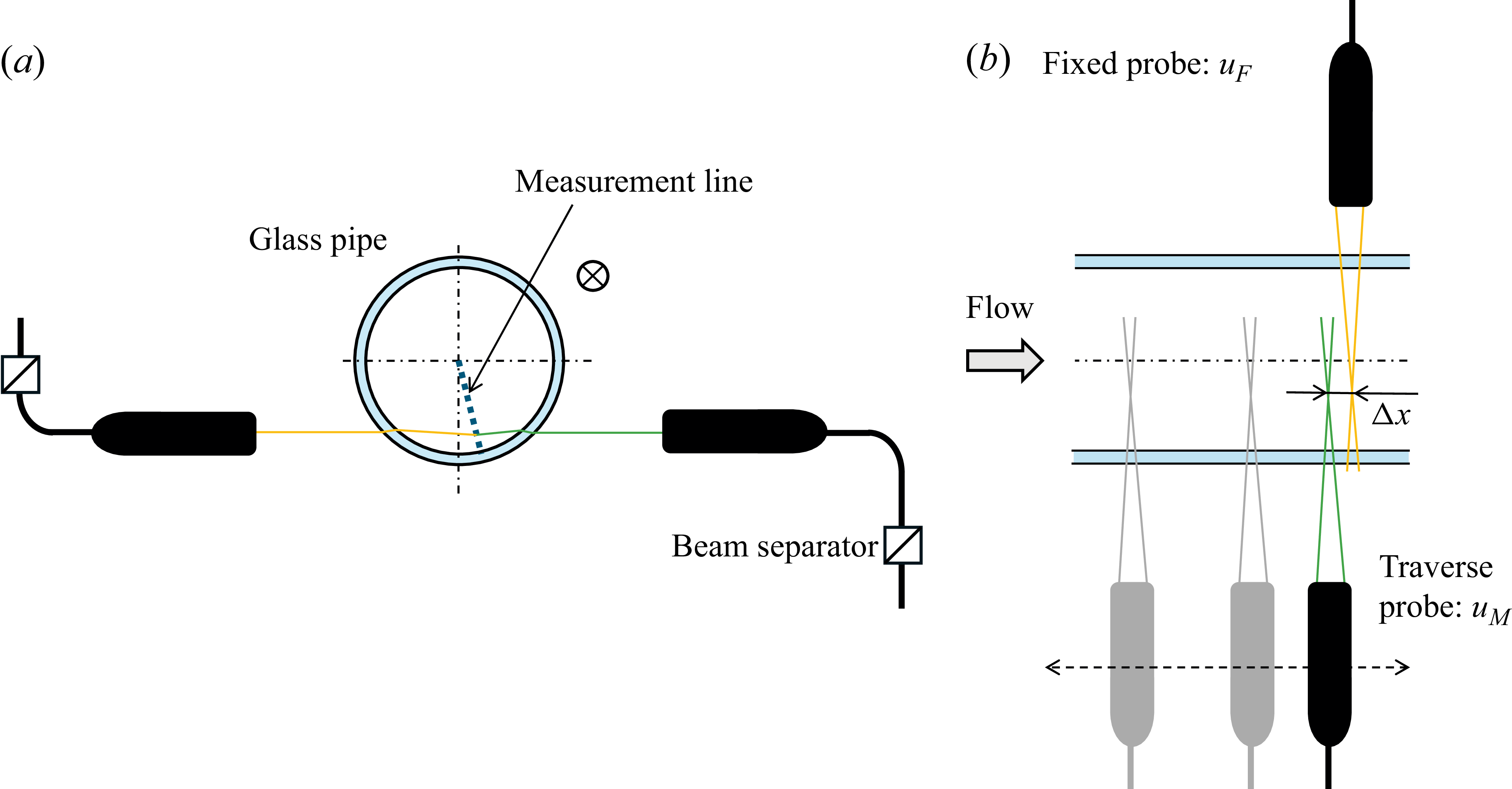
Measurement positions and LDV probe layout: (a) cross-sectional view and (b) top view. The wall-normal measurement positions are along the measurement line, which is slightly inclined relative to the angle of the laser beam insertion. The traverse probe was moved upstream.

In this experiment, two-point simultaneous measurements in the streamwise direction were conducted using two LDV systems, as shown in figure 2, and the convection velocity was estimated from the correlation between two time-series velocity components. The use of multiple LDV systems to obtain such correlations is a valid non-contact method and has therefore been applied since early studies (e.g. Morton & Clark Reference Morton and Clark1971). Cenedese, Romano & Di Felice (Reference Cenedese, Romano and Di Felice1991) and Romano (Reference Romano1995) applied this technique to channel flow and attempted to measure the convection velocity. However, these studies were limited to low Reynolds numbers and only a few measurement points, and thus did not address the convection velocity profile or its relationship to the large-scale structures.
Two laser beams were introduced from opposite sides, as shown in figure 2(b). One LDV probe, using a 561 nm wavelength laser, was fixed in place, while the other probe, using a 532 nm laser, was mounted on a traverse mechanism. Each measurement was performed using backscattering. Table 1 shows the streamwise distance between two measurement points,
 $\Delta x$
. Hereinafter,
 $\Delta x$
is referred to as the two-point distance. The velocity component measured by the fixed LDV system is denoted as
 $u_{\textit{F}}$
and that obtained by the traversing probe is denoted as
 $u_{\textit{M}}$
. An example of time-series velocity fluctuations measured simultaneously using two LDVs is shown in figure 3. A clear delay between the two time-series velocity signals is observed, not only for the large-scale structures but also for the small-scale structures.
Streamwise distance between two measurement points.

Example of raw data at
 $y^+=1500$
,
 $\Delta x/R=1$
and
 ${\textit{Re}}_{{\tau}}=14\,400$
. The black line represents
 $u_{\textit{M}}$
(traverse probe) and red line represents
 $u_{\textit{F}}$
(fixed probe). Here,
 $t$
is the time and
 $U$
is the local mean velocity.

Based on the principle of LDV, the velocity can only be measured when particles pass through the measurement volume. The frequency at which particles pass is random; therefore, a constant sampling interval, as used in hot-wire measurements, is not possible with LDV. This randomness is one of the significant issues when calculating the convection velocity from correlation coefficients. To address this issue, the mean sampling rate was kept as high as possible in the present experiment. The mean sampling rate ranged from 3 to 10 kHz, depending on the Reynolds number.
It should be noted that equally spaced sampling data are required to calculate correlation coefficients from experimental measurements. In this experiment, such data were reconstructed using the sample-and-hold method proposed by Adrian & Yao (Reference Adrian and Yao1986). The authors have previously applied this method to spectral analysis and confirmed its validity through comparison with results obtained using the hot-wire method (Ono et al. Reference Ono, Furuichi and Tsuji2025). The reconstructed time-series data were used for all analyses presented in this paper. The sampling interval of the reconstructed data was 50
 $\unicode{x03BC} {\textrm{s}}$
for
 ${\textit{Re}}_{{\tau}}=3000$
and 20
 $\unicode{x03BC} {\textrm{s}}$
for the other cases. The duration time
 $t$
was set to
 $tU/R \gt 10\,000$
in all experiments, which is sufficiently long to capture the large-scale structures with length of
 $10R-20R$
.
Figure 2(a) also shows the measurement positions used to obtain the convection velocity profile. These positions in the wall-normal direction are arranged along the measurement line, which is inclined by approximately
 $15^{\circ }$
relative to the direction of laser insertion. Due to the shape and refractive index of the glass pipe, it is impossible to reach the laser near the wall along a diameter line perpendicular to the insertion angle of the beam. This limitation is similar to the inability to measure near the wall using image-processing methods. On the other hand, the laser can be inserted near the wall along a diameter line that is shifted circumferentially by more than a certain angle from the perpendicular line to the beam insertion angle, as shown in figure 2. In this study, this limit was approximately
 $12^{\circ }$
–
 $13^{\circ }$
. At angles greater than this, velocity measurements near the wall become possible; however, the larger the angle, the worse the spatial resolution becomes. The angle used in this study (approximately
 $15^{\circ }$
) was selected as the measurable angle that minimises this effect while providing sufficient signal strength. In this experiment, the profiles were measured from
 $y/R=0.002$
to the pipe centre. The expanded uncertainty of velocity measurement with this LDV is approximately 0.2 % (
 $k$
= 2). The measurement length (spatial resolution) is
 $L_{\textit{u}}^+=27$
at
 ${\textit{Re}}_{{\tau}}=8860$
,
 $L_{\textit{u}}^+=59$
at
 ${\textit{Re}}_{{\tau}}=20\,800$
for
 $y^+=400$
. For details, see Ono et al. (Reference Ono, Furuichi, Kurihara, Wada and Tsuji2022, Reference Ono, Furuichi and Tsuji2023). It should be noted that, without a window chamber, the laser path would pass through air, glass and water, requiring a larger inclination angle of the measurement line, which would degrade the spatial resolution.
2.3. Calculation procedure for convection velocity
To calculate the convection velocity from experimental data, several methods can be considered. When multi-point data in the streamwise direction are available – such as image-processing techniques or pulsed ultrasonic Doppler methods – the convection velocity can be estimated from the two-dimensional spectrum (e.g. Furuichi, Takeda & Kumada Reference Furuichi, Takeda and Kumada2003; LeHew et al. Reference LeHew, Guala and McKeon2010; Cui & Jacobi Reference Cui and Jacobi2024). For two-point measurements, such as in the present study, the cross-correlation method is generally employed. The correlation coefficient
 $R(\Delta t)$
, where
 $\Delta t$
is lag time, is calculated as follows:
 \begin{equation} R(\Delta t)=\frac {\overline {u^{\prime}_{\textit{F}}(t+\Delta t)u^{\prime}_{\textit{M}}(t)}}{\sqrt {\overline {u^{\prime 2}_{\textit{F}}}}\sqrt {\overline {u^{\prime 2}_{\textit{M}}}}}, \end{equation}
where
 $u^{\prime}_{\textit{F}}$
and
 $u^{\prime}_{\textit{M}}$
denote fluctuations. An example of the time-dependent correlation coefficient is shown in figure 4. A clear delay in the correlation is observed, and this delay increases with the distance between the two measurement points.
Example of correlation coefficient as a function of delay time at
 $y^+=1500$
and
 ${\textit{Re}}_{{\tau}}=14\,400$
. The lines correspond to
 $\Delta x/R = 0.06$
, 0.12, 0.3, 0.5 and 1 shown in black, brown, red, orange and pink, respectively.

The convection velocity is determined using the following equation:
 \begin{equation} U_{\textit{cv}}=\Delta x/\Delta t_{\textit{p}}, \end{equation}
where
 $\Delta t_{\textit{p}}$
is the delay time corresponding to the peak of the correlation coefficient. As the two-point distance increases, the peak value of the correlation coefficient decreases due to the deformation of the turbulence structures. This attenuation with increasing separation is related to the Lagrangian correlation coefficient (Romano Reference Romano1995), although this aspect is not discussed here. The attenuation is particularly significant in the near-wall region. In the present study, data with a peak correlation coefficient below 0.15 were excluded from the analysis. This threshold was chosen based on the observation that convection velocities calculated under such conditions tend to exhibit large deviations compared with those at adjacent measurement points.
3. Experimental results and scaling of convection velocity
3.1. Convection velocity profile
In this section, we present the measurement results of the full-field convection velocity, obtained from the raw velocity signals, and examine its scaling. Before discussing the results, a comparison is made with previous studies. Krogstad et al. (Reference Krogstad, Kaspersen and Rimestad1998) measured the convection velocity in the TBL using the same procedure, in which the streamwise distance between two measurement points was varied. Figure 5 shows a comparison between the present results and those of Krogstad et al. (Reference Krogstad, Kaspersen and Rimestad1998). Note that the comparison is made using the ratio of the convection velocity to either the centreline velocity
 $Uc$
or the free-stream velocity
 $Ue$
, to account for the mismatch in Reynolds numbers. The Reynolds numbers in the comparison are
 ${\textit{Re}}_{{\theta}}=1409$
for Krogstad et al. (Reference Krogstad, Kaspersen and Rimestad1998) and
 ${\textit{Re}}_{{\tau}}=3000$
for the present study.
Variation of full-field convection velocity with
 $\Delta x/R$
measured by two-point correlation. Red symbols indicate the present results at
 ${\textit{Re}}_{{\tau}}=3000$
and black symbols represent the data from Krogstad et al. (Reference Krogstad, Kaspersen and Rimestad1998) at
 ${\textit{Re}}_{{\theta}}=1409$
. Here,
 $Uc$
and
 $Ue$
denote the centreline and free-stream velocities, respectively. The wall-normal positions are:
 :
 $y/R=0.74$
,
 :
 $y/R=0.20$
,
 :
 $y^+=32$
for the present study; and
 $\blacksquare$
:
 $y/\delta =0.77$
,
 $\blacktriangledown$
:
 $y/\delta =0.24$
,
 $\bullet$
:
 $y^+=38$
for Krogstad et al. (Reference Krogstad, Kaspersen and Rimestad1998), where
 $\delta$
is the boundary-layer thickness.

The results in the near-wall region (
 $y^+\approx 30$
) show good agreement. The results in the outer region (
 $y/R\approx 0.2$
and 0.7) exhibit good consistency for
 $\Delta x/R \gt 0.3$
(or
 $\Delta x/\delta \gt 0.3$
); however, significant deviations are observed for
 $\Delta x/R \lt 0.3$
(or
 $\Delta x/\delta \lt 0.3$
). In the result of Krogstad et al. (Reference Krogstad, Kaspersen and Rimestad1998), the convection velocity increases with
 $\Delta x$
at all wall-normal positions, whereas in the present study, it remains nearly constant in the outer region. Considering the agreement at large
 $\Delta x$
, the discrepancy may be attributed to the influence of the upstream probe. In the experiment by Krogstad et al. (Reference Krogstad, Kaspersen and Rimestad1998), the upstream probe at
 $y^+=38$
, referred to as the ‘inner probe’, was mounted protruding from the wall into the flow, so that its influence on the downstream measurement was minimal. However, in the outer region, the upstream probe – referred to as the ‘outer probe’ – was inserted directly into the flow, making it difficult to avoid interference with the downstream measurement. Choi & Moin (Reference Choi and Moin1990) reported a comparison between DNS and experiments using a hot-wire, regarding the dependence of convection velocity on measurement distance. Their results show the same trend: the convection velocity from DNS is higher than that from experiments when the measurement distance is small. This finding supports the present results shown in figure 5. However, Krogstad et al. (Reference Krogstad, Kaspersen and Rimestad1998) also investigated the influence of upstream probes and found it to be small. Therefore, further research is required to determine whether the observed difference is indeed due to probe interference.
Full-field convection velocity profiles and their deviations from the local mean velocity at (a,b)
 ${\textit{Re}}_{{\tau}}=3000$
(red), (c,d)
 ${\textit{Re}}_{{\tau}}=8860$
(orange), (e, f)
 ${\textit{Re}}_{{\tau}}=11\,200$
(purple), (g,h)
 ${\textit{Re}}_{{\tau}}=14\,400$
(green) and (i,j)
 ${\textit{Re}}_{{\tau}}=20\,800$
(black). Symbols represent the normalised two-point distance
 $\Delta x/R$
:
 $\triangle$
: 0.06,
 $\diamond$
: 0.12,
 $\square$
: 0.3,
 $+$
: 0.5,
 $\circ$
: 1. The solid lines in the left-hand panels indicate the mean velocity profile from Ono et al. (Reference Ono, Furuichi, Kurihara, Wada and Tsuji2022). Grey shaded areas denote the logarithmic regions in the mean velocity profiles. The short- and long-alternating dotted lines in (d) and (j) are the fitting lines for
 $\Delta x/R=1$
.

The full-field convection velocity profiles for each
 $\Delta x$
and Reynolds number are shown in figure 6, along with deviations from the local mean velocity. The grey shaded areas indicate regions where the logarithmic behaviour is clearly observed in the mean velocity profile; these are highlighted for high Reynolds numbers (
 ${\textit{Re}}_{{\tau}} \geq 8860$
). The experimental results for the convection velocity shown in figure 6 are smooth and follow the same general level as the mean velocity, although slight scatter is observed at small
 $\Delta x$
and
 ${\textit{Re}}_{{\tau}}=11\,200$
. Overall, the convection velocity is nearly consistent with the local mean velocity from the logarithmic region to the pipe centre. In the near-wall region, on the other hand, the convection velocity tends to exceed the local mean velocity, remaining approximately constant. These trends are generally consistent across all Reynolds numbers examined. For instance, the convection velocity at
 $y^+=50$
and
 ${\textit{Re}}_{{\tau}}=20\,800$
is approximately 30 % larger than the local mean velocity.
The profile shape is first discussed from the outer region. Beyond a certain wall-normal position, referred to as the transition point
 $y_{\textrm{T}}$
, the convection velocity becomes independent of the two-point distance
 $\Delta x$
. In this region, the convection velocity is generally consistent with the local mean velocity, as reported in previous studies even at low Reynolds numbers (
 ${\textit{Re}}_{{\tau}}\lt 2000$
) (e.g. del Álamo and Jiménez Reference del Álamo and Jiménez1982; Österlund et al. Reference Österlund, Lindgren and Johansson1990; Liu & Gayme Reference Liu and Gayme2020; Mehrez et al. Reference Mehrez, Yamamoto and Tsuji2023). Strictly speaking, these earlier studies found that the convection velocity in the outer region is slightly lower than the local mean velocity. Similarly, in the present study, at
 ${\textit{Re}}_{{\tau}}=3000$
, the convection velocity is slightly lower than local mean velocity, whereas at higher Reynolds numbers, it appears to be slightly higher. Although this may suggest a weak Reynolds-number dependence, the observed differences are within the range of the measurement uncertainty. Therefore, the present study does not assert that the convection velocity in the outer region is exactly equal to the local mean velocity.
Next, the inner region is discussed. For
 ${\textit{Re}}_{{\tau}} \leq 11\,200$
, the convection velocity clearly depends on the two-point distance
 $\Delta x$
within the region inside the transition point. As
 $\Delta x$
increases, the convection velocity also increases, and around
 $\Delta x/R=0.5$
, the convection velocity profile becomes nearly independent of the wall-normal position. This position-independent region lies farther inward than the logarithmic region of the mean velocity profile. These trends are observed in figure 5 and are consistent with previous studies (Bull Reference Bull1967; Choi & Moin Reference Choi and Moin1990; Krogstad et al. Reference Krogstad, Kaspersen and Rimestad1998). According to Krogstad et al. (Reference Krogstad, Kaspersen and Rimestad1998), when the two-point distance is short, the observed correlation is dominated by small-scale structures, whose convection velocity is approximately equal to the local mean velocity. However, as these small-scale structures deform during downstream advection, their correlation weakens, and the contribution from large-scale structures becomes dominant. The convection velocity associated with large-scale structures is known to be higher than that of small-scale structures (del Álamo and Jiménez Reference del Álamo and Jiménez1982; Kim & Hussain Reference Kim and Hussain1993). Therefore, the interpretation reported by Krogstad et al. (Reference Krogstad, Kaspersen and Rimestad1998) is considered plausible and supports the view that the near-wall position independence of the convection velocity profile is linked to the influence of large-scale structures. On the other hand, at higher Reynolds number
 ${\textit{Re}}_{{\tau}} \leq 11\,200$
, the dependence on the two-point distance becomes weaker.
Reynolds-number dependence of the full-field convection velocity profile at (a)
 $\Delta x/R=0.12$
, and (b)
 $\Delta x/R=1$
at
 ${\textit{Re}}_{{\tau}}=3000$
(red), 6070 (blue), 8860 (orange), 11 200 (purple), 14 400 (green) and 20 800 (black). The colours and symbols are the same as those in figure 6. The red short- and long-alternating dotted line represents the convection velocity obtained by DNS from Geng et al. (Reference Geng, He, Wang, Xu, Lozano-Durán and Wallace2015) at
 ${\textit{Re}}_{{\tau}}=932$
. The grey filled circles represent data obtained by input–output analysis from Liu & Gayme (Reference Liu and Gayme2020) at
 ${\textit{Re}}_{{\tau}}=1000$
. The black solid line represents the convection velocity of small-scale structures (
 $\lt 2h$
, where
 $h$
is the channel half-width) obtained by DNS from del Álamo and Jiménez (Reference del Álamo and Jiménez1982) at
 ${\textit{Re}}_{{\tau}}=1900$
, and the blue broken line represents the convection velocity of pressure fluctuations obtained by DNS from Mehrez et al. (Reference Mehrez, Yamamoto and Tsuji2023) at
 ${\textit{Re}}_{{\tau}}=2000$
.

The Reynolds-number dependence of the convection velocity is shown in figure 7. Figure 7(a) shows the result at
 $\Delta x/R=0.12$
and figure 7(b) is
 $\Delta x/R=1$
. For comparison, previous results are also included. In figure 7(a), we show the convection velocity obtained by DNS at
 ${\textit{Re}}_{{\tau}}=932$
from Geng et al. (Reference Geng, He, Wang, Xu, Lozano-Durán and Wallace2015) by DNS, by input–output analysis at
 ${\textit{Re}}_{{\tau}}=1000$
from Liu & Gayme (Reference Liu and Gayme2020) and by DNS at
 ${\textit{Re}}_{{\tau}}=1900$
from del Álamo and Jiménez (Reference del Álamo and Jiménez1982) for small-scale structures (
 $\lt 2h$
, where
 $h$
is the channel half-width). In addition, the convection velocity of pressure fluctuations reported by Mehrez et al. (Reference Mehrez, Yamamoto and Tsuji2023) at
 ${\textit{Re}}_{{\tau}}=2000$
by DNS is also included. Except in the near-wall region, the present data at the lowest Reynolds number (
 ${\textit{Re}}_{{\tau}}=3000$
) agree well with all these previous results. In the near-wall region, the profile exhibits a constant-value plateau, as already noted. The convection velocity associated with this plateau increases in magnitude and extends farther from the wall with increasing Reynolds number. This trend is consistent with earlier findings; in particular, the previous results at
 ${\textit{Re}}_{{\tau}}=3000$
and those of Mehrez et al. (Reference Mehrez, Yamamoto and Tsuji2023) at
 ${\textit{Re}}_{{\tau}}=2000$
show close agreement. These consistencies lend support to the validity of the present measurements at
 $\Delta x/R=0.12$
. By contrast, at
 $\Delta x/R=1$
, the near-wall difference becomes more pronounced, and the resulting convection velocity is not fully consistent with the previous studies shown here. One possible reason for this inconsistency is that increasing the two-point distance enhances the contribution of large-scale structures to the correlation, as discussed. A comparison of the convection velocity for large-scale structures between the previous study and the present results at
 $\Delta x/R=1$
is presented in § 3.2.
As shown in figure 7, the convection velocity profile at low Reynolds numbers with
 $\Delta x/R=0.12$
almost agrees with previous studies; however, noticeable difference emerges at higher Reynolds number and
 $\Delta x/R=1$
. The most significant discrepancy at high Reynolds numbers lies in the location of the transition point,
 $y_{\textrm{T}}$
. In the present results,
 $y_{\textrm{T}}$
is located approximately in the middle of the logarithmic region of the mean velocity profile – for example,
 $y_{\textrm{T}}^+ \approx 650$
at
 ${\textit{Re}}_{{\tau}}=8860$
and
 $y_{\textrm{T}}^+ \approx 2200$
at
 ${\textit{Re}}_{{\tau}}=20\,800$
. These positions are determined from the zero-crossing point of the fitting line at
 $\Delta x/R=1$
, as shown in figures 6(d) and 6(j). In contrast, earlier studies have typically observed the transition point to be much closer to the wall, at most around
 $y^+ \approx 100$
(e.g. del Álamo and Jiménez Reference del Álamo and Jiménez1982). At the low Reynolds number of
 ${\textit{Re}}_{{\tau}}=3000$
and
 $\Delta x/R=0.06$
, the transition point in the present study appears consistent with earlier findings, but clear deviations are observed under other conditions.
3.2. Scaling of full-field convection velocity
In this section, we discuss the scaling of the full-field convection velocity obtained from two-point correlation measurements. Although the convection velocity roughly follows the mean velocity profile, a definitive scaling has not yet been established, and the issue remains under debate. It is generally accepted that the convection velocity exceeds the local mean velocity in the near-wall region and approaches it in the outer region. However, previous studies have reported substantial discrepancies. For example, Atkinson et al. (Reference Atkinson, Buchmann and Soria2015) did not observe a constant convection velocity region near the wall, in contrast to the findings of del Álamo and Jiménez (Reference del Álamo and Jiménez1982). In the outer region, we have already noted differences between the present results and those of Krogstad et al. (Reference Krogstad, Kaspersen and Rimestad1998) at the same
 $\Delta x/R$
. These examples highlight the variability among studies. Krogstad et al. (Reference Krogstad, Kaspersen and Rimestad1998) suggested that the scale dependence of the convection velocity contributes to this scatter, which is plausible, but the absence of a unified framework for interpreting the convection velocity profile is likely another factor.
The present study provides convection velocity profiles over a wide range of Reynolds numbers, offering a valuable basis for developing a scaling law. Figure 7 presents a first attempt: the convection velocity, normalised in inner units at fixed
 $\Delta x/R$
. In the outer region, the profiles collapse well, similar to the mean velocity. By contrast, in the inner region, a clear Reynolds number dependence persists, demonstrating that the scaling in figure 7 is not sufficient.
Scaling of full-field convection velocity with respect to
 $\Delta x^+$
; (a)
 $\Delta x^+=600{-}900$
and (b)
 $\Delta x^+=5000{-}8000$
. Colours and symbols are the same as in figure 6. The lines in (a) are the same as in figure 7, and the broken line in (b) indicates the present result for
 $\Delta x^+=20\,000$
.

Figure 8 shows the full-field convection velocity profiles scaled by introducing the inner variable for the two-point distance,
 $\Delta x^+$
 $(=u_{{\tau}} \Delta x/\nu )$
. Because identical values of
 $\Delta x^+$
cannot be achieved for all Reynolds numbers under the present experimental conditions, data at Reynolds numbers as close as possible are grouped for the comparison. The range
 $\Delta x^+=600{-}900$
is shown in figure 8(a) and
 $\Delta x^+=5000{-}8000$
in figure 8(b). In both cases, the profiles collapse well and show no Reynolds-number dependence. These results indicate that the convection velocity can be scaled in the (
 $x^+-y^+$
) plane. In other words, the convection velocity varies systematically with both wall-normal position and two-point distance in inner units. As described in § 3.1, the two-point correlation primarily reflects the convection velocity of structures that dominate the correlation, which depends on
 $\Delta x^+$
. The present findings therefore suggest the relevant structures – and thus their convection velocities – change with
 $\Delta x^+$
, highlighting a scale dependence tied to the underlying structures.
The solid line in figure 8(a) represents the full-field convection velocity prolife for small-scale structures (
 $\lt 2h$
) reported by del Álamo and Jiménez (Reference del Álamo and Jiménez1982). This profile agrees well with the present results, except near the wall, suggesting that the convection velocity obtained from the two-point correlation at
 $600\lt \Delta x^+\lt 900$
is primarily influenced by small-scale structures. In contrast, the broken line shown in figure 8(b) shows the profile for
 $\Delta x^+ \approx 20\,000$
obtained in the present study. This profile is nearly identical to those at
 $\Delta x^+=5000{-}8000$
in the outer region, indicating that the convection velocity there is independent of
 $\Delta x^+$
and exhibits universal behaviour. In the inner region, however, a weak
 $\Delta x^+$
-dependence remains. del Álamo and Jiménez (Reference del Álamo and Jiménez1982) reported that this region can be scaled using the bulk velocity,
 $U_{\textit{b}}$
. Figure 9 shows the profile of
 $U_{\textit{cv}}/U_{\textit{b}}$
at
 $\Delta x/R=1$
, i.e. in outer scaling. The convection velocity collapses well across Reynolds numbers, particularly in the near-wall region (
 $y/R\lt 0.02$
) where the convection velocity is nearly constant. For large
 $\Delta x^+$
, the appropriate scaling for the near-wall region is therefore confirmed by outer scaling with the bulk velocity. In the outer region, both scalings in figures 8(b) and 9 appear to work reasonably well. Within the present Reynolds-number range, it is not possible to conclude which scaling is more suitable for the outer region at large
 $\Delta x$
.
Full-field convection velocity scaled with the bulk velocity at
 $\Delta x/R=1$
. Colours and symbols are the same as figure 6. The black solid line represents the convection velocity for large-scale structures (
 $\gt 2h$
) from del Álamo and Jiménez (Reference del Álamo and Jiménez1982).

For comparison, figure 9 also includes the profile for large-scale structures (
 ${\gt}2h$
) reported by del Álamo and Jiménez (Reference del Álamo and Jiménez1982), which shows good agreement with the present results in the inner region. As discussed in § 3.1, a large two-point distance
 $\Delta x$
is expected to enhance the contribution of large-scale structures to the correlation in the near-wall region. The agreement between the
 ${\gt}2h$
structures of del Álamo and Jiménez (Reference del Álamo and Jiménez1982) and the present results at
 $\Delta x/R=1$
in the near-wall region supports this interpretation. In the outer region, by contrast, the two profiles do not coincide; however, in light of the preceding discussion, the outer-layer behaviour at large
 $\Delta x$
may be better represented by inner scaling.
4. Discussion on convection velocity of VLSMs and LSMs
4.1. Convection velocity associated with VLSMs
Very large-scale motions, which have a characteristic size of approximately
 $10R-20R$
, appear prominently at high Reynolds numbers. Since the velocity fluctuations induced by VLSMs constitute one of the largest contributions to the turbulence intensity (e.g. Baars & Marusic Reference Baars and Marusic2020), many researchers have focused on understanding their mechanisms. The VLSMs have been primarily investigated through spectral analysis, and numerous studies have been reported in the literature (e.g. Marusic et al. Reference Marusic, McKeon, Monkewitz, Nagib, Smits and Sreenivasan2010a; Vallikivi et al. Reference Vallikivi, Ganapathisubramani and Smits2015; Ono et al. Reference Ono, Furuichi and Tsuji2025). An interesting debate exists regarding the spectral features associated with VLSMs. del Álamo and Jiménez (Reference del Álamo and Jiménez1982) argued that the spectral peak in PMS related to VLSMs is an artefact resulting from Taylor’s frozen turbulence hypothesis. When they applied their proposed correction to Taylor’s hypothesis, the VLSM associated spectral peak attenuated. However, Rosenberg et al. (Reference Rosenberg, Hultmark, Vallikivi, Bailey and Smits2013) applied the same correction method to high-Reynolds-number pipe flow and reported that no significant reduction in the VLSM-related peak was observed. Furthermore, a comparison of PMS distributions from DNS and experimental data (based on Taylor’s hypothesis) by Monty & Chong (Reference Monty and Chong2009) observed discrepancy in the higher wavenumber region. They attributed this inconsistency to an insufficient domain length in the DNS. These discussions highlight the importance of accurately determining the convection velocity, particularly in the context of evaluating the validity of Taylor’s hypothesis in relation to VLSMs.
As mentioned in the introduction, previous studies have reported that convection velocity exhibits scale dependence. This dependence is particularly evident in the near-wall region, where the convection velocity associated with large-scale structures is higher than that of smaller-scale structures. These large-scale structures referenced in earlier studies are often interpreted as representations of VLSMs. However, it remains unclear whether they strictly correspond to VLSMs. For instance, del Álamo and Jiménez (Reference del Álamo and Jiménez1982) reported the convection velocity for structures larger than
 $2h$
(see figure 9). However, their analysis was conducted at a Reynolds number of
 ${\textit{Re}}_{{\tau}}=1900$
, which is too low for VLSMs to be clearly observed, as shown in the previous PMS contour maps (e.g. Marusic et al. Reference Marusic, McKeon, Monkewitz, Nagib, Smits and Sreenivasan2010a
; Yamamoto & Tsuji Reference Yamamoto and Tsuji2018). While VLSMs are generally characterised by streamwise lengths of the order of
 $10R-20R$
, structures of around
 $2R$
are typically classified as LSMs (Kim & Adrian Reference Kim and Adrian1999). Therefore, it remains uncertain whether the large-scale structures examined by del Álamo and Jiménez (Reference del Álamo and Jiménez1982) correspond to VLSMs or rather to LSMs. This motivates further examination of the convection characteristics of VLSMs at higher Reynolds numbers.
In this section, the convection velocity associated with VLSMs is estimated through scale separation of the velocity fluctuation. The threshold frequency for the separation is determined from the measured convection velocity, and the scale-separated spectrum is converted back into time-series data using inverse Fourier analysis (see figure 11 for an example of reconstructed velocity fluctuations). The same analysis is applied to velocity signals measured at two spatially separated points, and the convection velocity is then calculated from the cross-correlation of the reconstructed time-series data. A key aspect of this method is the appropriate choice of the threshold frequency, which is essential for clearly isolating the convection velocity of VLSMs. In the present study, scale separation is used to distinguish between large-scale (VLSM) and medium-scale (LSM) motions. Specifically, the convection velocity of structures larger than
 $5R$
– denoted as
 $U_{\textit{cv-L}}$
– is taken to represents VLSMs, while that of structures between
 $0.5R$
and
 $5R$
– denoted as
 $U_{\textit{cv-M}}$
– represents medium-scale structures, including LSMs. It should be noted that both VLSMs and LSMs are often grouped together under the term ‘large-scale structures’ in previous studies. For example, Mathis, Hutchins & Marusic (Reference Mathis, Hutchins and Marusic2011) defined large-scale structure as
 $\lambda ^+\gt 7000$
, which corresponds to approximately
 $1.15R$
at
 ${\textit{Re}}_{{\tau}}=6070$
and
 $0.35R$
at
 ${\textit{Re}}_{{\tau}}=20\,800$
. These values are roughly consistent with the lower bound of the medium-scale range defined above. Expressed in inner variables, the definitions become
 $\lambda ^+\gt 30\,400$
for the large scale and
 $3040\lt \lambda ^+\lt 30\,400$
for the medium scale at
 ${\textit{Re}}_{{\tau}}=6050$
,
 $\lambda ^+\gt 104\,000$
for the large scale and
 $10\,400\lt \lambda ^+\lt 104\,000$
for the medium scale at
 ${\textit{Re}}_{{\tau}}=20\,800$
.
Typical results of the scale-separated convection velocities are shown in figure 10(a) for
 ${\textit{Re}}_{{\tau}}=20\,800$
and
 $\Delta x/R=1$
. For medium-scale structures, the convection velocity
 $U_{\textit{cv-M}}$
is nearly identical to
 $U_{\textit{cv}}$
obtained from the raw velocity signal. This trend is consistently observed at other Reynolds numbers and
 $\Delta x$
values, indicating that most of the results reported in § 3 primarily reflect the convection velocity of such medium-scale structures. In contrast, for structures larger than
 $5R$
, the convection velocity
 $U_{\textit{cv-L}}$
is higher than
 $U_{\textit{cv-M}}$
and remains nearly constant across a wide range of wall-normal positions. Specifically, the constant convection velocity region extends up to approximately
 $y^+\lt 2000$
. Ono, Furuichi & Tsuji (Reference Ono, Furuichi and Tsuji2024) reported the distribution of PMS at high Reyolds numbers, showing that the VLSM-dominated region extends from
 $y^+ \approx 150$
to
 $y^+ \approx 2000$
at
 ${\textit{Re}}_{{\tau}}=20\,800$
. The agreement between the constant convection velocity region and the VLSM-dominated region suggests that the convection velocity
 $U_{\textit{cv-L}}$
has been appropriately subtracted from the raw signals. It is also worth noting that VLSMs have been reported to influence the near-wall turbulence intensity through what is known as a footprint effect (Mathis et al. Reference Mathis, Marusic, Chernyshenko and Hutchins2013). Therefore, the observation of a constant convection velocity extending towards the near-wall region is not inconsistent with the behaviour expected of VLSMs.
(a) Scale-separated convection velocity at
 ${\textit{Re}}_{{\tau}}=20\,800$
and
 $\Delta x/R=1$
. Symbols show:
 $\circ$
, full-field convection velocity;
 $\times$
, scale-separated convection velocity
 $U_{\textit{cv-M}}^+$
for medium-scale structure (
 $0.5R-5R$
);
 $\triangledown$
, scale-separated convection velocity
 $U_{\textit{cv-L}}^+$
for large-scale structure (
 $\gt 5R$
). Broken line indicates
 $23u_{{\tau}}$
. Grey shaded area represents the logarithmic region of mean velocity profile. (b) Scale-separated convection velocity
 $U_{\textit{cv-L}}^+$
at
 $\Delta x/R=1$
for various Reynolds numbers. Colours are the same as in figure 6. The broken line represents
 $0.85U_{\textit{b}}$
.

The Reynolds-number dependence of scale-separated convection velocity for structures larger than
 $5R$
is shown in figure 10(b) for
 ${\textit{Re}}_{{\tau}} \geq 6050$
. Although some scatter is observed near the wall, the convection velocity
 $U_{\textit{cv-L}}$
remains nearly constant and shows no significant dependence on Reynolds number when scaled by the bulk velocity. These results indicate that the constant convection velocity associated with VLSMs can be effectively scaled by the bulk velocity, and it is estimated to be
 $0.85U_{\textit{b}}$
.
The above results clearly indicate that the convection velocity is scale-dependent, and caution must be exercised when applying Taylor’s hypothesis for the inner region, as also noted in previous studies. In particular, the convection velocity of large-scale structures, including VLSMs, is greater not only than the local mean velocity but also than the convection velocity estimated from two-point correlation. This deviation becomes more pronounced closer to the wall. Consequently, if the local mean velocity is used as the convection velocity, the wavenumber of VLSMs will be underestimated.
In the outer region, by contrast, the convection velocity of structures larger than
 $5R$
is smaller than both the local mean velocity and unfiltered convection velocity. Although its relation to large-scale structures remains unclear, it is evident that the convection velocity in the outer region also exhibits scale dependence. Therefore, even in the outer region – where the convection velocity roughly matches the local mean velocity – Taylor’s hypothesis cannot be reliably applied using a single, unified convection velocity for large-scale structure.
4.2. Further discussion on convection velocity of LSM
In the above discussion, we focused on the mean convection velocity. It is of interest to consider the extent to which Taylor’s frozen turbulence hypothesis can be applied on the basis of this mean convection velocity. However, reconstructing the velocity field using the mean convection velocity is generally challenging. Dennis & Nickels (Reference Dennis and Nickels2008) and Atkinson et al. (Reference Atkinson, Buchmann and Soria2015) reported discrepancies between velocity fields reconstructed using the mean convection velocity and the corresponding measured fields. These findings are well supported by the observations of Adrian et al. (Reference Adrian, Meinhart and Tomkins2000), who used PIV measurement in the TBL. They showed that small-scale vortices in the shear layer are not accurately captured using Reynolds decomposition. Instead, such scale-dependent structures can be more effectively extracted when the local convection velocity – defined within the local streamwise–wall-normal plane – is employed. This clearly indicates that the convection velocity varies both spatially and temporally. Moreover, it is believed that the convection velocities of small-scale structures are strongly influenced by LSMs. In this section, we further investigate the temporal fluctuations of convection velocity associated with large-scale structures, which reflect the underlying spatio-temporal dynamics of the flow structures.
Reconstructed velocity signals for (a)
 $u_{\textit{F}}$
and (b)
 $u_{\textit{M}}$
at
 $y^+=1500$
,
 $\Delta x/R=1$
and
 ${\textit{Re}}_{{\tau}}=20\,800$
. The black lines indicate high-speed segments for (
 $u_{\textit{F-H}}$
,
 $u_{\textit{M-H}}$
), while the grey lines indicate low-speed segments (
 $u_{\textit{F-L}}$
,
 $u_{\textit{M-L}}$
). The orange lines show the large-scale components
 $u_{\textit{F-VL}}$
and
 $u_{\textit{M-VL}}$
, extracted for structures larger than
 $5R$
.

Spatio-temporal features are generally extracted by applying conditional sampling based on specific events in the velocity fluctuations. A similar approach can be applied to the temporal characteristics of convection velocity. For example, the convection velocity associated with events such as sweeps and ejections has been investigated (Krogstad et al. Reference Krogstad, Kaspersen and Rimestad1998; Dróżdż et al. Reference Dróżdż, Niegodajew, Romańczyk and Elsner2015). In this section, we focus on the convection velocity associated with events related to the motion of VLSMs. Figure 11 illustrates the schematic procedure used to extract the velocity fluctuations associated with VLSMs. This figure shows two simultaneously measured velocity signals and highlights the large-scale fluctuation component (structure size
 $\gt 5R$
), denoted as
 $u_{\textit{F-VL}}$
, which is obtained in § 4.1. Based on this reconstructed large-scale fluctuation, the raw velocity signal upstream proves
 $u_{\textit{F}}(t)$
is decomposed into high-speed and low-speed components as follows:
 \begin{align} u_{\textit{F-H}}(t) & = \begin{cases} u_{\textit{F}}(t) & u_{\textit{F-VL}}(t)\geq U ,\\ U & u_{\textit{F-VL}}(t)\leq U, \end{cases} \end{align}
 \begin{align} u_{\textit{F-L}}(t) & = \begin{cases} u_{\textit{F}}(t) & u_{\textit{F-VL}}(t)\leq U ,\\ U & u_{\textit{F-VL}}(t)\geq U, \end{cases} \end{align}
where
 $U$
is the local mean velocity. The same decomposition is applied to the velocity signal from the downstream probe
 $u_{\textit{M}}(t)$
. Subsequently, cross-correlations are calculated separately for the high-speed segments (
 $u_{\textit{F-H}}$
and
 $u_{\textit{M-H}}$
) and the low-speed segments (
 $u_{\textit{F-L}}$
and
 $u_{\textit{M-L}}$
) to estimate the corresponding convection velocities.
This procedure can be interpreted in the context of the uniform momentum zone (UMZ). In previous studies on UMZs (e.g. Adrian et al. Reference Adrian, Meinhart and Tomkins2000), snapshots of the velocity vector field in the streamwise–wall-normal (
 $x{-}y$
) plane have been shown to consist of distinct zones characterised by nearly uniform momentum or velocity. From the perspective of pointwise temporal measurements, different UMZs pass the measurement location over time. When this concept is considered together with VLSMs, high-speed and low-speed zones are seen to pass alternately, leading to large-amplitude velocity fluctuations. Such alternating regions of high and low speed have also been observed in PIV measurements by Dennis & Nickels (Reference Dennis and Nickels2011).
Time-resolved correlation coefficients for reconstructed velocity signals associated with VLSM. The red line represents the high-speed segment (
 $u_{\textit{F-H}}$
,
 $u_{\textit{M-H}}$
), the bule line represents the low-speed segment (
 $u_{\textit{F-L}}$
,
 $u_{\textit{M-L}}$
) and the broken line corresponds to the raw velocity signal.

Figure 12 shows the time-series correlation coefficients corresponding to figure 11. From the time delay between the positive and negative peaks of the correlation, the characteristic streamwise scale of the structures can be estimated. For the raw velocity signal, this scale is approximately
 $10R$
, whereas for both reconstructed signals (high-speed and low-speed segments), the estimated scale is approximately
 $2R$
. This suggests that the convection velocity obtained from the reconstructed data reflects the motion of LSMs. As discussed in § 4.1, the convection velocity of LSMs is broadly comparable to or equal to the local mean velocity in the outer region. However, the observed difference in the lag time between the high- and low-speed segments indicates that the convection velocity associated with structures including LSM varies over time.
Time-resolved convection velocity at
 ${\textit{Re}}_{{\tau}}=20\,800$
and
 $\Delta x/R=1$
. Symbols show:
 $\bullet$
, time-resolved convection velocity for high-speed segment;
 $\circledcirc$
, time-resolved convection velocity for low-speed segment;
 $\circ$
. full-field convection velocity. The solid line represents the mean velocity profile, and the grey shaded area indicates the logarithmic region.

The convection velocities corresponding to reconstructed data, namely time-resolved convection velocities, are shown in figure 13. These results clearly demonstrate that the convection velocity is higher in the high-speed segment and lower in the low-speed segment. This difference is particularly evident in the range of approximately
 $300\lt y^+\lt 3000$
, which spans the logarithmic region of the mean velocity profile and coincides with the VLSM-dominated region. The influence of this variation diminishes both toward the wall and toward the pipe centre. These findings indicate that the convection velocity of LSM-scale structures varies in response to the fluctuations associated with VLSMs, providing clear evidence that the convection velocity changes temporally. Moreover, even structures of similar size exhibit different convection velocities depending on whether they reside in the high- or low-speed segments associated with VLSMs.
Finally, we provide some comments on the outer region (
 $y/R\gt 0.2$
or
 $y^+\gt 4000$
at
 ${\textit{Re}}_{{\tau}}=20\,800$
). As shown in figure 6, the full-field convection velocity closely matches the local mean velocity in this region. Moreover, large-scale structures associated with VLSMs are generally no longer dominant here. Nevertheless, the results in figure 13 indicate that the influence of VLSM-scale large structures on the convection velocity can still be observed, even in the outer region. Similarly, figure 10(a) shows scale-dependent behaviour of the convection velocity in this region. Although it remains unclear whether VLSMs directly affect the flow in the outer region, these results suggest that caution is required when applying Taylor’s frozen turbulence hypothesis – even in the outer region of wall-bounded flows.
5. Conclusion
In this study, the convection velocity in high-Reynolds-number pipe flow was measured using two-point correlations. Velocity measurements were conducted using two LDV systems. The Reynolds number was in the range
 ${\textit{Re}}_{{\tau}}=3000{-}20\,800$
, and the convection velocity profile was obtained from
 $y/R=0.002$
to the pipe centre. To the best of our knowledge, such detailed profile measurements of the convection velocity in high-Reynolds-number pipe flow have not been reported previously. Therefore, the present results provide valuable data for discussions on the conversion from frequency to wavenumber domains based on Taylor’s frozen turbulence hypothesis. Additionally, we investigated the convection velocity associated with VLSMs, which become increasingly prominent at high Reynolds number.
The full-field convection velocity profiles, obtained from the raw velocity signal, agree well with previous results for channel flows and the TBL at lower Reynolds numbers, showing higher velocities than the local mean velocity near the wall and converging toward the local mean velocity farther from the wall. A key difference at high Reynolds number is that the region where the convection velocity matches the local mean velocity is shifted farther from the wall – appearing from the middle of the logarithmic region to the pipe centre – compared with previous studies. Furthermore, we demonstrated that the convection velocity can be scaled using inner variables, namely
 $y^+$
and
 $\Delta x^+$
, suggesting that the convection velocity depends on the spatial distance over which it is evaluated through two-point velocity fluctuations.
The VLSM-scale structures were extracted by scale separation. Velocity fluctuations associated with structures larger than
 $5R$
were isolated, and their convection velocities were calculated from the correlation coefficients of reconstructed time-series velocity data. The scale-separated convection velocity was found to be higher than the unfiltered values and remained nearly constant across a wide region up to
 $y^+\lt 2000$
at
 ${\textit{Re}}_{{\tau}} \approx 20\,000$
. Since this range corresponds well with the region dominated by VLSMs, the measured convection velocity is considered to accurately reflect the behaviour of VLSMs. Moreover, this constant convection velocity region scales well with the bulk velocity, approximately
 $0.85U_{\textit{b}}$
. In contrast, the convection velocity for structures in the range of
 $0.5R$
to
 $5R$
, which includes LSMs, closely matches full-field convection velocity.
Finally, convection velocities were calculated from velocity signals decomposed into high- and low-speed segments associated with VLSM. It was found that the time-resolved convection velocities of these two segments differ within the VLSM-dominant region. This suggests that, when applying Taylor’s frozen turbulence hypothesis, it is essential to account not only for the scale dependence of the convection velocity but also for its temporal fluctuations, which reflect the underlying spatio-temporal dynamics of the flow structures. In particular, the convection velocity of LSM-scale structures (approximately
 $2R$
) was found to fluctuate significantly over time, depending on the velocity fluctuations associated with VLSMs. This finding implies that structures of similar size can exhibit different convection velocities depending on their surrounding flow conditions. Although incorporating this variability into Taylor’s hypothesis remains challenging at present, these results highlight the need for deeper consideration when applying wavenumber–frequency conversion to single-point measurements.
Funding
This research was partially supported by JSPS KAKENHI Grant Numbers JP22K04943.
Declaration of interests
The authors report no conflict of interest.