

1 Introduction
Pay-as-you-go (PAYG) pension systems have recently come under severe pressure from demographic developments that might jeopardize long-run fiscal sustainability. The demographic challenge is primarily the result of constantly increasing life expectancy and of large swings in fertility rates. In many industrialized countries, e.g., the baby boom of the 1960s has been followed by a remarkable bust in later decades and a general decline in the birth rate. It is forecasted that these changes will lead to a considerable increase in the old-age dependency ratio (for the EU15, e.g., from 25% in 2003 to 52% in 2050).Footnote 1 This has caused doubts about the sustainability of current PAYG pension systems and has initiated various efforts to reform these systems, either via more piecewise, parametric reforms or via the introduction of ‘notional defined contribution’ (NDC) systems as in Sweden (cf. Disney, Reference Disney1999; Palmer, Reference Palmer2000; Lindbeck and Persson, Reference Lindbeck and Persson2003; Barr and Diamond, Reference Barr and Diamond2006). In Germany, a sustainability factor has been introduced in 2003 in order to deal with the demographic challenge (cf. KNFSS, 2003; Börsch-Supan et al., Reference Börsch-Supan, Reil-Held and Wilke2003).Footnote 2
In this paper, we study the properties and characteristics of sustainability factors that are similar to real-world counterparts, in particular to the German prototype. This is done within the framework of a stylized multiperiod model of a PAYG pension system. The automatic adjustment factors specify how the contribution rate and the pension level have to be altered in reaction to changes in the dependency ratio in order to keep the budget of the pension system in balance. A parameter α determines whether the adjustment to demographic fluctuations is primarily achieved by changing the contribution rates or by changing the pension levels. This set-up includes a defined contribution (DC) system (α=1) and a defined benefit (DB) system (α=0) as nested cases. The German sustainability factor, for example, stipulates an adjustment parameter of α=0.25.Footnote 3 The choice of the adjustment weight is obviously a crucial issue that determines how the adjustment burden is distributed among different generations. Despite its importance for the design of new and the reform of established pension systems, not much work exists on this issue. The multiperiod structure allows us to derive results that are less stylized than the findings from related two-period models and directly applicable to real-world pension systems.
We study how the choice of α determines which generation bears the main burden of adjustment when cohort sizes fluctuate. For this purpose, we use the internal rate of return (IRR) as our measure of intergenerational distribution. Given the focus of the paper, we look at the PAYG system in isolation and we abstract from all other potential sources of old age income. We show that the IRR can be approximated in a simple and compact form as an additive function of the deviation of a sequence of cohort sizes from some reference cohort size. In particular, the IRR of some generation t might be influenced by a large number of cohorts that starts from the one that dies just after generation t has entered the labor market and reaches up to the cohort that begins to work when generation t is in the last year of its retirement. The elasticity with which the rate of return reacts to the size of a different cohort depends on life expectancy, the retirement age, and (in a linear fashion) on the distance of this cohort from period t. It can be shown that these elasticities always sum up to zero, implying that the IRR for a generation is not affected if there is only a general change in the size of all cohorts. Furthermore, it can be shown that if the cohort sizes increase over time at a constant rate, then the IRR is simply given by the growth rate of the wage bill. This is in fact the expected result since the growth rate of the wage bill is the ‘biological interest rate’ of a PAYG system. For the general case of a non-constant development of cohort sizes, however, the elasticities of the IRR can be used to distinguish between different adjustment regimes and to guide the choice of the crucial weighting parameter α.
We find that the smallest total sensitivity to changes in the cohort sizes is associated with an adjustment parameter that is given by the quotient of the retirement period to the total time spent in the pension system. Assuming, for example, that people work for 45 years and spend 15 years in retirement, then the sum of the absolute elasticities is smallest for α=0.25. Taking an ex-ante (or ‘behind the veil of ignorance’) perspective, one can also look at the constant parameter value that minimizes the total variance of the IRR when the cohort size follows a stationary stochastic process. In this case, the expected value of the IRR is independent of the chosen adjustment policy, and a risk-averse individual will choose the policy that involves the smallest fluctuations in the IRR. We find that this minimum variance adjustment parameter lies between α=0.29 and α=0.38 (depending on the assumption about the length of working life and retirement). Taken together these results thus suggest that the choice of the German adjustment weight could in fact be justified by arguments that refer to a low sensitivity of the IRR to fluctuations in cohort size.Footnote 4
The analysis also shows that adjustment regimes with a fairly constant contribution rate (large α) are more ‘forward looking’ (i.e., the IRR reacts more strongly to the size of succeeding generations than to the size of preceding) than frameworks with fairly stable pension levels (small α). Forward-looking schemes thus have the property that the IRR is to a larger degree influenced by the size of cohorts for which a generation is at least partly responsible. At the end of the paper, we discuss briefly what this property could mean for the desirability of different adjustment policies.
The paper is organized as follows. In the next section, we discuss the related literature while, in Section 3, we present the multiperiod model of the PAYG pension system where we also define the sustainability factor and calculate the IRR corresponding to different specifications of the adjustment factor. In Section 4, we proceed to analyze the consequences of this sustainability factor for issues of intergenerational distribution and burden-sharing. Section 5 concludes.
2 Related literature
The analysis of this paper is related to a number of studies that deal with the issue of risk-sharing and intergenerational distribution in PAYG systems. This literature includes among others the papers by Hassler and Lindbeck (Reference Hassler and Lindbeck1997), Thøgersen (Reference Thogersen1998), Bohn (Reference Bohn, Campbell and Feldstein2001), and Wagener (Reference Wagener2003, Reference Wagener2004). Thøgersen (Reference Thogersen1998), for example, uses a two-period OLG model with constant population growth and an exogenously given process for wages. Individual (ex-ante) utility is assumed to depend on net lifetime income and on the variance of this income. It is shown that a DC policy is able to provide intergenerational risk-sharing, while a DB policy increases the income risk of all generations. Wagener (Reference Wagener2003) has challenged this result by using a different (ex-post) welfare criterion and by allowing for optimal (savings) decisions. He also uses, however, a deterministic process for population growth. Bohn (Reference Bohn, Campbell and Feldstein2001) considers various forms of risk, including demographic risks (shocks to the birth rate and to life expectancy). He shows that in the case of shocks to the birth rate a DB system is ex-ante more efficient since it better allows to offset the effects of factor price movements. The results are again derived in a two-period setting and only the extreme cases of complete DB and complete DC are considered. Wagener (Reference Wagener2004) studies the optimal combination of changes in the contribution rate and changes in pension benefits. He shows that (under the assumption of a fixed population) typically both older and younger individuals will prefer a mixture of the two systems (i.e. a parameter 0<α<1). Breyer and Kifmann (Reference Breyer and Kifmann2004), finally, deal explicitly with the German pension formula and they focus on its properties in the presence of increases in life expectancy. They deal both with questions of intragenerational equity (due to group-specific differences in life expectancy) and with intergenerational issues (due to trends in population growth and longevity).
In addition to this class of papers that use two-period set-ups, there also exists a literature that is based on multiperiod OLG models. Krüger and Kubler (Reference Krüger and Kubler2006), for example, study the question of whether the introduction of a PAYG system might lead to a Pareto improvement if financial markets are incomplete. More related to our topic, Fehr and Habermann (Reference Fehr and Habermann2006) compare the effects of a ‘sustainability factor’ and a ‘demographic factor’ in a setting with a stochastic demographic development that is calibrated to the German situation. Both factors are based on specific reform proposals for Germany and the sustainability factor is in fact similar to our formulation (where the adjustment parameter is fixed at α=0.25). They find that both factors will benefit future generations and harm middle-aged generations and that the effects are larger for the sustainability factor. They do not study, however, the impact of the sustainability factor for different weights α and they use utility-based welfare measures instead of the IRR in order to compare different policies.
This brief literature overview indicates that the framework of this paper shows similarities and differences to the existing literature along four dimensions. First, we focus on fluctuations in the demographic structure and hold wage growth constant. Second, we look at the IRR to judge the effects of demographic fluctuations on intergenerational distribution and risk-sharing, thereby abstracting from eventual behavioral changes. Third, we work with a multiperiod model that allows us to study more realistic demographic patterns (like boom-and-bust cycles). Forth, we allow for a continuum of adjustment polices and do not focus only on the extreme cases of a DB or a DC policy. As discussed above, none of these factors is a unique feature of our paper. What distinguishes it from the existing literature, is the combination of these four specific modeling assumptions that allow for some new results and a complementary view on the issue of risk-sharing and intergenerational distribution in the presence of demographic fluctuations.
Our results are likely to change if we allowed for more types of shocks (e.g. productivity shocks or life expectancy shocks) or if we also took possible behavioral changes (concerning saving, labor supply and fertility) into account. We do not believe, however, that these changes would overturn our main findings concerning the impact of different adjustment policies on the intergenerational distribution of demographic shocks. Extensions along these lines are in any case a promising field for future research.
3 The model
3.1 Set-up
The size of the generation born in time t is denoted by N t. We assume that each generation works for G periods, receives a pension for M periods, and dies after Y=G+M periods. G, M, and Y are assumed to be constant across generations and M⩽G. The wage and pension in time t are denoted by w t and p t, respectively. In a specific period of time, all workers and pensioners receive the same payment (i.e. there is no seniority structure). In each working period, the representative member of a cohort pays a contribution rate τt. Given the focus of the paper, we only look at the PAYG system in isolation. This means that we do not explicitly consider other forms of old age income (like a funded pension pillar or private savings) and we treat labor supply and fertility decisions as exogenously given. These assumptions allow us to deal with the multiperiod model in an analytically tractable and intuitive way. Allowing for optimizing individuals and their behavioral responses to different policy designs would be a worthwhile and challenging extension of the present paper.
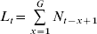
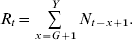
The total number of workers L t and the total number of retired persons R t at time t is given by
The dependency ratio z t is defined as the quotient of pensioners to workers

For later reference, we also define the (relative) pension level q t by

The pension level thus indicates which fraction of average income the representative member of a generation receives in a given year of his or her retirement. The growth rate of wages g t+1 is given by

and we write the size of the different cohorts as

In equation (6), ηt can be a interpreted as a known value that is used to describe the pattern of the population. Or, alternatively, one can also think of ηt as a stochastic term that is ex-ante uncertain and that is distributed with zero mean and variance σ η2. We will use both interpretations in the following. Finally, we assume that the budget of the pension system is balanced in every period. The income of the pension system in time t is given by w tτtL t, while the total expenditures are given by p tR t=w tq tR t. Thus, the balanced budget condition (BBC) can be written as

A ‘demographic steady state’ is defined as a situation where the working population is constant, that is N t= , ∀t. From (1), (2) and (7), it follows that the BBC reduces to τtG=q tM. The steady state dependency ratio for a constant population, a constant retirement age G, and a constant life expectancy Y comes out as
 . Denoting the steady state level of the contribution rate and the pension level by
 and
 , respectively, the BBC (7) implies the following relation

The values for and can be freely chosen as long as (8) is fulfilled.
3.2 The automatic adjustment factor
The automatic adjustment factor states how the contribution rate and the pension level have to be changed when the dependency ratio z t changes. This factor can be expressed formally in the following way

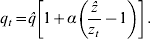
Equations (9) and (10) determine how the adjustment to an increase in the dependency ratio z t is borne by workers and pensioners. If α=0, the pension level is held constant at and thus the full burden of adjustment to demographic fluctuations is shouldered by the working population via changes in the contribution rate. This corresponds to the defined benefit (DB) case. The reverse is true for α=1, where the contribution rate stays constant at and solely the pension level is varied to achieve a balanced budget. This refers to the defined contribution (DC) case. In general, α determines how the ‘demographic burden’ is shared between contributors and pensioners. In 2003, Germany introduced an automatic adjustment factor similar to (9) and (10) (and termed it the ‘sustainability factor’) for which the relative adjustment weight was set equal to α=0.25 (cf. KNFSS, 2003 and Börsch-Supan et al., Reference Börsch-Supan, Reil-Held and Wilke2003, 15).Footnote 5 It is straightforward to show that a pension system characterized by (9) and (10) leads to a constantly balanced budget.Footnote 6
3.3 Definition of the internal rate of return
There exist various measures of intergenerational distribution that can be used to evaluate the distributional properties of existing pension schemes and the effects of proposed pension reforms. Four widely used measures are the IRR, the present value ratio, the net present value, and the implicit tax rate (cf. Geanakoplos et al., Reference Geanakoplos, Mitchell, Zeldes, Mitchell, Myers and Young1999; Fenge and Werding, Reference Fenge and Werding2003). In this paper, we want to focus on the IRR since it is a commonly used indicator in this context. The IRR has the additional advantage that it does not require a decision about an appropriate discount rate. The implicit tax rate, however, which is also frequently used to assess the intergenerational distribution, depends on the choice of the discount rate, which is a controversial issue. For the special case where the discount rate is assumed to be equal to the growth rate of the economy, it can be shown, however, that the main properties of the IRR and the implicit tax rate are basically identical (see Appendix B.2).
The IRR δk for generation k is defined as the rate that equates the present value of benefits to the present value of contributions. In formal terms

In the rest of the paper, we assume that wages grow at a constant rate, that is g t=g, ∀t. Using this in (11) together with (4) leads to a simple implicit definition of the IRR:  . If we use the linear approximation
 , we can find a closed-form solution for the generation-specific IRR δk

3.4 The internal rate of return implied by the automatic adjustment factor
In Appendix B.1, we show how one can use a Taylor approximation (around N t+j=, ∀j) of (12) to write the IRR in a compact and intuitive form. We summarize the result in the following proposition.
Proposition 1
If a pension system uses the adjustment factors given in equations (9) and (10) and if the development of cohort sizes is given by equation (6), then the IRR of generation k can be approximated as
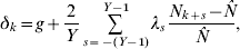
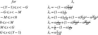
where λs is a piecewise linear function of s given by
It holds that
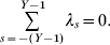
The coefficient λs can be interpreted as the (semi-)elasticity of the IRR δk with respect to the deviation of cohort size N k+s from the reference cohort size . A value of λ20=0.02 indicates, for example, that (for Y=60) the IRR increases by 0.67 percentage points if the size of cohort N k+20 is 10% larger than . Let us consider three particular assumptions concerning the development of cohort sizes:
• If N t is constant at some level
 (where is sufficiently close to such that the approximation in (13) holds), then it follows from (13) and (14) that δk=g. In other words, for a constant population the IRR is simply given by the growth rate of wages g.
• If we interpret ηt in (6) as a stochastic process with E(ηt)=0 and Var(ηt)=ση2, then we can conclude from (13) that E(δk)=g. The expected IRR of a system where the size of the population follows a stationary stochastic process is constant and independent of the adjustment policy used (i.e., independent of the parameter α).
• In the literature, one can often find the assumption of a constantly growing population. If we assume N t=(1+n)tN 0 instead of (6), we can use (12) to calculate that δk=g+n (see Appendix B.1). In this case, the IRR equals the growth rate of the wage bill g+n. This is in fact the famous result, first derived by Samuelson (Reference Samuelson1958), that population growth in a PAYG system works like a ‘biological interest rate’.
 (where
The cases where the population is constant or constantly growing are, however, not the most interesting ones. First, the results for these cases are well known and have already been discussed in the literature. Second, the empirically more relevant situations involve cohort sizes that change from year to year in an irregular manner and where, for example, periods with large cohorts are followed by periods with smaller cohorts (‘baby boom and bust cycles’). For a discussion of this situation the linear approximation in (13) is particularly convenient since it allows a direct comprehension of the distributional consequences of fluctuating cohort sizes.
It is useful to start the discussion with the two-period model. As can be seen from (13), in general the generations from −(Y−1) to +(Y−1) might exert an influence on the IRR. For the two-period model (Y=2), this means that generation k can only be affected by the size of the own cohort and by the sizes of the directly preceding and the directly succeeding generation (N k−1 and N k+1, respectively). From the formulas for λs in proposition 1, the elasticities for the three cohorts can be calculated as λ−1=−(1−α), λ0=1−2α, λ1=α. In the DB case (α=0), it is only the past and present generations that count since the relative size of these two cohorts determines the contribution rate that generation k has to pay during its active period. For the DC case (α =1), however, only the sizes of the present and the future generation matter since their proportion is decisive for the pension level that generation k will receive in old age. For intermediate cases (0<α<1), all three generations are important where the exact magnitude of the impact depends on the parameter α. For  , the size of the own cohort N k does not matter since the positive effect (more contributors to pay for the pensions of the old generation) and the negative effect (more pensioners that have a claim on the total contributions paid by the young generation) just cancel.
The main logic of the two-period case carries over to the multiperiod context. Nevertheless, the two-period model is quite special since it assumes that work and retirement are of the same length. Furthermore, in the two-period case, there are no generational overlaps in the working and in the pension period and accordingly also no possible counteracting effects of specific cohort sizes. The multiperiod model offers a more complex and more complete picture that is intimately related and immediately comparable to real-world situations and can be used to analyze specific developments, such as boom and bust cycles. In the next section, we want to look at this case from two different angles. First, we will present the different ‘cohort dependence structures’ associated with different adjustment policies; second, we will study how sensitive the IRR is to fluctuations in the cohort size and how a hypothetical social planner might choose among the different policies.
4 Properties of the internal rate of return
4.1 Cohort size dependence under different adjustment factor specifications
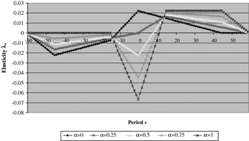
The pattern of intergenerational linkages that is present in the formulas for the elasticities λs can best be illustrated by the use of a specific numerical example. This is done in Figure 1 for five different values of α and under the assumption that G=45, M=15, and Y=60. These values broadly conform to the case of the ‘standard pensioner’ that is often used to assess properties of the real-world pension system. The standard pensioner is a fictitious person who enters the labor market at the age of 20, works at the average wage for exactly 45 years, and retires at the statutory retirement age of 65. In addition, the numerical example is based on an assumed life expectancy of 80 years, which is close to the current value for Germany.Footnote 7 Later we will sometimes also refer to two alternative numerical examples where we assume that individuals retire at the age of 60 (that is G=40, M=20, Y=60) or where we assume that they retire at the age of 60 and enter the labor market at the age of 25 and (that is G=35, M=20, Y=55).
Elasticity (λs) of the Internal Rate of Return of Generation k (δk) to the Size of Different Cohorts (Nk+s)

The one characteristic of these figures that immediately catches the eye is that the patterns look quite different and that the intergenerational distribution seems to depend heavily on the parameter α. Every pension scheme thus involves some underlying (explicit or implicit) ‘cohort dependence structure’. An important distinguishing characteristic of the different curves is that they cut the zero line at different values. This means that the adjustment parameter α determines which cohort sizes have a positive or a negative influence on a generation's IRR. In the next proposition, we summarize some properties of this cut-off value.
Proposition 2
(i) For each generation k, the IRR δkis unaffected by the size of one specific cohort
in −M⩽⩽M for which .(ii) for
, this cut-off cohort is the own cohort, that is .(iii) for
, the cut-off cohort is given by , while, for , we have that . It follows that . Furthermore, for (), it holds that >0 () and λ0<0 (λ0>0).
 in −M⩽
 .
 , this cut-off cohort is the own cohort, that is
 .
 , the cut-off cohort is given by
 , while, for
 , we have that
 . It follows that
 . Furthermore, for
 (
 ), it holds that
 ) and λ0<0 (λ0>0).
Proof:
See Appendix B.3. As stated in proposition 2, for  the elasticity with respect to the size of the own generation is zero, while the elasticities with respect to generations that have been born before (after) themselves are negative (positive). The weight
 is given by the fraction of the total life span that is spent in retirement, that is
 . For the two-period case, the cut-off value is thus given by
 =0.5, while for the example of Figure 1, it comes out as
 . The own cohort is working for G periods (thereby increasing the contribution base) and receives a pension for M periods (thereby reducing the volume of available pension funds) and, for
 , these two effects exactly cancel each other. For
 , the size of the own cohort has a negative net effect (that is λ0<0) since the fact that more people are in retirement at the same time now outweighs the effect that more people are contributing during the working years. The identity of the cohort
 , for which the two effects exactly neutralize each other (that is for which
 =0), depends on the magnitudes of G, M, and α as stated in part (iii) of proposition 2. For α=0, for example, it is given by
 and for α=1 by
 .Footnote 8 This cut-off value
 increases in the parameter α as is also visible in Figure 1. The parameter
 will be important later when we discuss the sensitivity of the IRR to fluctuations in the cohort size.
In order to understand the intuition behind the shape of the elasticities, it is useful to discuss one of the two benchmark cases more extensively. For the DC case (α=1), the contribution rate is fixed at  for all times and thus members of generation k do not care about the dependency ratio while they are working. This changes, however, once they retire in period k+45 (that is k+G) since then the relative sizes of L and R have an impact on their pension levels. When they reach retirement age, there are 14 older generations that are already receiving pensions. The more numerous these pensioner cohorts are, the lower will be the relative pension and the IRR of generation k. If the size of the pensioners aged 79 (cohort k−14) is large, then this is not so dramatic since they will only be around for one more year and will thus only depress the pension level for one year of the total retirement span. This is different, however, for the cohort that is only one year older (generation k−1). They will be alive almost for the whole pension period of generation k and will accordingly lower the pension level for 14 years. The worst impact on the IRR of generation k is, however, the size of the own cohort, as shown in Figure 1, where for α=1 the negative impact is largest for cohort size N k.
Possible negative effects can of course be counterbalanced if the work force is large during generation k's retirement period. This is, however, a double-edged sword. If cohort k+1 is large, this is not very helpful since generation k will gain nothing from this large size until they are retired. Then, however, they have only one year to benefit from the large size of cohort k+1 since a year later the latter will retire themselves from when on they will depress the relative pensions of generation k for 14 additional years. As shown in Figure 1, the net effect of a large cohort N k+1 is clearly negative. In fact, this net effect stays negative up to cohort k+12.Footnote 9 Generation k will prefer a situation where the large cohorts are the ones that contribute to the pension system for a long time while being at the same time young enough so that they will only reach retirement age when generation k is already dead and gone. Cohorts k+15 to k+44 will pay contributions for the entire time when generation k is in pension and thus their impact on the IRR is largest and identical as shown by the straight segment in Figure 1. For generations that are still younger (k+45 to k+59), this positive impact weakens since generation k will die before it can reap the full benefits of eventual larger cohort sizes. The intuition for the opposite case with α=0 (DB) and policies with different α's is similar.Footnote 10
4.2 The impact of fluctuations in the cohort size on fluctuations in the IRR
PAYG systems are often studied under the perspective of risk-sharing and intergenerational insurance. As discussed briefly in Section 2, the existing literature has so far concentrated primarily on fluctuations in wages and it has mostly used two-period models to analyze the risk-sharing properties of DB (α=0) and DC (α=1) models. In the present paper, we take a somewhat different approach since we focus on fluctuations in cohort sizes in a multiperiod framework. We want to investigate which adjustment policy will minimize the sensitivity of the IRR with respect to fluctuations in the cohort size. We will deal with two measures of variability: the variance of the IRR and the sum of absolute values of the elasticities λs.Footnote 11 The latter measure is useful in this context since it reflects the total effect that variations in the cohort size might have on the IRR, irrespective of the specific assumptions concerning the stochastic process of the cohort sizes. The following proposition summarizes some crucial properties of this measure.
Proposition 3
Let  . It holds that
 . Therefore, |λ|sumhas a minimum at
 where it is given by |λ|sum=1.
Proof:
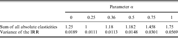
See Appendix B.4. The sum of the absolute value of the elasticities λs as defined in Proposition 3 gives a useful indication of the total potential effect of fluctuations on the IRR. In the first line of Table 1, we report the measure |λ|sum for our numerical example of Figure 1 (M=15, Y=60) and for six values of α (including the de facto value for the German system of α=0.36). It is largest for α=1 and smallest for α=0.25. In fact, it is shown in Proposition 3 that it is not only true that |λ|sum=1 for α=0.25 for this specific example but holds for every case where  . For the two alternative numerical examples, the parameter values that minimize |λ|sum are given by α=0.33 (for M=20, Y=60) and α=0.36 (for M=20, Y=55), respectively.
Summary of Elasticties for Special Groups of Cohorts
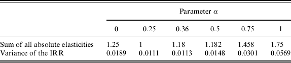
Note: The table is based on the example with M=15, G=45 and Y=60. The first line shows the sum |λ|sum of the absolute value of all elasticities λs. The second line shows the (normalized) variance Var(δk)/ση2 of the internal rate of return δk.
The second indicator of the receptiveness of the IRR to fluctuations in cohort size is its variance. In this case, we interpret again the development of cohort sizes in (6) as a stochastic process where ηt is an i.i.d. shock. The next proposition summarizes the main properties.
Proposition 4
The variance of the IRR is given by  . The α for which the variance is at a minimum can be calculated as

for  , we have that
 .
Proof:
See Appendix B.5. Using equation (15), we can calculate the variance-minimizing value of α for various extreme assumptions about the length of retirement M and the life span Y. For M=0 (no retirement), we get αMinVar=0; for  (equal share of work and retirement), we have
 ; and for M=Y (no work),
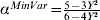 . For ‘reasonable’ values of Y and M, however, we get that αMinVar is smaller than 0.5 and in general close to
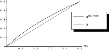
 . For Y=60 and M=15, for example, it comes out as αMinVar=0.295 (while =0.25).Footnote 12 This is illustrated in Figure 2, where we plot αMinVar and for
 . As indicated in Proposition 4 only for
 and for the degenerate case with M=0, the minimum-variance value for α is in fact given by . Figure 2 shows, however, that αMinVar is always fairly close to .
In the second row of Table 1, we report the variance for the six values of α. We observe that the variance for α=0.25 and α=0.36 is not much different from the minimum variance value at αMinVar=0.295, where it is given by 0.0109. If we use the two alternative numerical examples, we get αMinVar=0.37 (for M=20, Y=60) and αMinVar=0.39 (for M=20, Y=55), respectively.
Parameters for α that minimize the sensitivity of the IRR to fluctuations in cohort size

Summing up, we have seen in this section that for reasonable numerical values for the length of working life, the retirement age, and life expectancy (with Y between 55 and 60 and M between 15 and 20), an adjustment parameter between α=0.25 and α=0.39 seems to be an appropriate choice to achieve a low sensitivity of the IRR with respect to fluctuations in cohort sizes. These interval includes both the de jure German value of α=0.25 (for which the sum of absolute elasticities |λ|sum is lowest if M=15 and Y=60) and the de jure value of α=0.36 (which almost corresponds to αMinVar in the case where M=20 and Y=60).
4.3 The choice of an optimal adjustment factor
The results concerning the variance-minimizing value of α are also interesting since they can be interpreted from a social welfare perspective. In particular, one can assume a risk-averse individual (or social planner) who has to choose an adjustment policy ex-ante (behind the ‘veil of ignorance’) and who cares about the mean and variance of the IRR and abstracts from all behavioral decisions. Since the expected value of the IRR is independent of the adjustment parameter α (cf. Proposition 1), such a risk-averse individual behind the veil of ignorance will choose the adjustment policy that delivers the smallest variance given the stochastic process of population growth. In other words, it will choose the policy parameter αMinVar. Given this perspective the social planner will thus also choose a parameter between α=0.25 and α=0.39. Taken all together, the German weight of α=0.25 (or the de facto weight of α=0.36) is supported by these considerations. This justification based on a minimum-variance argument for the choice of the German adjustment parameter looks somewhat surprising since it does not seem to be the case that the choice has been primarily motivated by such principal considerations but rather by the pragmatic objective of keeping the contribution rate below some threshold value.Footnote 13
One should, however, be cautious not to stretch this result too far.
First, the choice of a constant α that minimizes the variance of the IRR is certainly not an uncontroversial criterion for a social planner. One could also try to find a complete path of αt (or, more generally, of generation-specific contribution rates and pension levels) that leads to identical IRRs for every cohort. Under this perspective, the task would thus be to come up with the smallest fluctuations in τt and q t that are able to deliver such a constant IRR. Our perspective, however, is exactly the mirror image in that we look for a constant α that is associated with the smallest fluctuations in the IRR. We have chosen this approach for two reasons. First, the adjustment factors (9) and (10) only require information about the current cohort size and no forecasted values. It is thus straightforward to implement the policy even in the presence of uncertainty about the future development of cohort sizes. Second, the German example and other existing PAYG systems indicate that transparency, reliability, and predictability are important properties of the pension system that are easier to accomplish with simple and sparsely parameterized schemes. Political economy arguments would further suggest that the choice of a single parameter α might be helpful to deal with potential problems of time inconsistency when policy makers might have an incentive to deviate ex-post from a path for αt that has looked optimal ex-ante. We leave a more extensive analysis of these interesting questions for future research.
A second qualification of the results of the paper has to do with the fact that the model concentrates on fluctuations in the cohort size and abstracts, for example, from stochastic productivity growth and also from increases in life expectancy. The latter issue is particularly relevant since over the last decade one could observe a steady increase in life expectancy by about 0.15 to 0.25 years in each calender year. For a constant retirement age M, such an increase in life expectancy Y will affect the IRR for each generation under every adjustment policy. A detailed analysis of this situation is, however, again beyond the scope of this paper. In particular, for this case of increasing life expectancy, one would have to consider an additional crucial policy parameter – the determination of the statutory retirement age. We would guess, however, that the broad implications of different parameter values α on the relative intergenerational distribution of different cohort sizes will stay qualitatively the same.
Furthermore, we have not taken explicit behavioral responses concerning savings, labor supply, and fertility into account. Our focus is the choice of an adjustment policy for a given pattern of behavioral responses and a given (deterministic or stochastic) demographic process. Even from this perspective, however, there exist additional criteria that could be taken into account when judging the choice of an adjustment regime. In particular, one can observe from Figure 1 that adjustment factors with a large α seem to be more ‘forward looking’ than DB policies, that is their IRR seems to be influenced to a larger extent by the size of future (succeeding) cohorts. This property might in fact be important in as far as it could be (and was) argued that fluctuations in the IRR between different generations might be justifiable by reference to their reproductive or ‘birth-promoting’ behavior. On an individual basis, there exists in fact an ongoing debate whether cohorts with a smaller numbers of descendants should shoulder a larger part of the demographic burden, both because they are partly responsible for the drop in the size of birth cohorts and because they are in a better (financial) situation to make good for the shortfall through private provisions. On an individual level, this argument amounts to linking the contributions and benefits to a person's number of children.Footnote 14
Under a collective (cohort-based) perspective, considerations concerning a reasonable and intergenerationally equitable pension system could thus be put forward to argue that the IRR should as strongly as possible be related to the number of children a cohort has produced. In particular, it could be stated that the IRR should primarily reflect the size of the cohorts of generation k's prospective children, that is approximately of generations k+20 to k+40. The negative financial consequences of a declining cohort size should be borne by the parent generation while – vice versa – the latter should also accredit gains from a possible increase.
Such a point of view would thus look more favorably towards a DC policy that shows the largest dependence on the size of these potential descendant generations. On the other hand, however, the difference with respect to this criterion between the policies with values for α between 0.25 and 1 are not very pronounced. Furthermore, it should be stressed that all adjustment policies involve also a reaction to the cohort size of preceding generations, which is not compatible with the argument that the IRR should reflect the pattern of collective responsibility. In order to include the argument of individual or collective responsibility into the model of a pension system, it would be necessary to explicitly introduce fertility decisions. An important aspect of such an extension would also be related to the trade-off between the quantity of children and their educational achievements. It might well be the case that the higher average human capital of relatively smaller generations offsets the detrimental impact of their pure size on the IRR.
5 Conclusion
In this paper, we have analyzed the properties of automatic adjustment factors that can be used to keep PAYG pension systems financially balanced in the case of fluctuations in cohort sizes. In order to study the implications of different adjustment factors on the intergenerational distribution, we have used the internal rate of return (IRR). We have shown that the IRR can be expressed as an additive function of the deviation of cohort sizes from some reference cohort size where the elasticity of the IRR of one cohort with respect to the size of some other cohort depends (inter alia) on the distance between the two generations.
We have used this simple and intuitive representation of the IRR to derive a number of results that are helpful in judging the distributional properties of existing practices and in guiding the choice of future policies. In this context we have stressed that it is important to take the highly dissimilar cohort dependence structure of different adjustment policies into account when deciding on the adjustment weight α. We have shown that the total effect on the IRR of fluctuations in the cohort size is smallest for a parameter that is equal to the fraction of the retirement period to the total time spent in the pension system. For reasonable numerical examples, the sum of the absolute elasticities is lowest for values between α=0.25 and α=0.36 and the smallest variance of the IRR will be observed for values of α between 0.29 and 0.39. The chosen weight for the German sustainability factor of α=0.25 (or de facto of α=0.36) can thus be interpreted as (intentionally or unintentionally) reflecting the choice of an adjustment policy that minimizes intergenerational fluctuations in the IRR.
Appendix A
A.1 Relation of (9) and (10) to the German sustainability factor
The German sustainability factor is closely related to equations (9) and (10). There exist, however, three differences between this formulation and its real-world pendant as mentioned in the text. In the following, we want to briefly discuss the most important difference. This refers to the fact that equation (10) is not fully accurate since in Germany a ‘modified gross earnings indexation’ is used that can be translated into the language of the model as followsFootnote 15

Increases in the contribution rate will thus lead to a slower adjustment of the pension value than specified in (10). The expression in terms of levels that corresponds to equation (16) can be written as
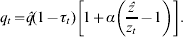
An adjustment regime given by (9) and (17) will work in exactly the same way as a regime that is determined by (9) and (10). The only difference is that the neat separation between the contribution rate and the pension level that is characteristic for the latter regime is not present in the first regime since here the contribution rate also enters the formula for the pension level. A change in the dependency ratio will thus have a direct effect on q t (via the term  ) and an indirect effect (via the effect on τt). In the following, we want to show that one can solve the system given by (9) and (17) and arrive at modified expressions for τt and q t.
We start by noting that using  in (7), we can write
 . Solving this for τt, we can derive that
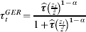
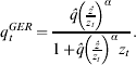
Note that τtGER⩽τt and q tGER⩽q t. This expression can be linearized around  to arrive at


where  . Using an automatic adjustment factor that is based on equations (9) and (17) will thus lead to results that are completely analogous to the results based on a pension system given by (9) and (10). The only difference is that one has to be careful in calibrating the model. Using the German choice of α=0.25 and the current German contribution rate of
 leads to a value of β=0.36. This is the de facto value inherent in the current German system that determines its degree of intergenerational burden-sharing.
Appendix B: Proofs
B.1 Proposition 1
The expression for δk in (12) can be written as  , where
 .
A Taylor approximation of δk around  , ∀j can be written as

Using (9) and (10), we can derive that for  , ∀j it holds that
 and thus
 and
 , ∀t. In this case,
 (this follows from (8)),
 and thus
 . Therefore,
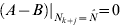 and thus also
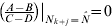 . Furthermore, we also have that
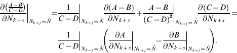
We can calculate that 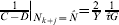 . Therefore
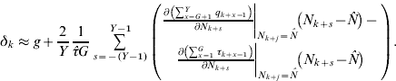
Note that in each of the summands in 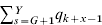 and
 , each cohort N k+s appears at most one time − either in L k+x−1 or in R k+x−1, depending on whether the cohort was part of the labor force or part of the pension cohorts in that specific period. For some period k+x, there exist therefore four possible effects:
• The reaction of τk+x to a change in N k+s if N k+s was part of L k+x in period k+x
• The reaction of τk+x to a change in N k+s if N k+s was part of R k+x in period k+x
• The reaction of q k+x to a change in N k+s if N k+s was part of L k+x in period k+x
• The reaction of q k+x to a change in N k+s if N k+s was part of R k+x in period k+x




So, if cohort (k+s) is large and if it is part of the pension cohorts in some period m, then it will increase the contribution rate in this period. If generation k is working in this period m and is thus affected by the increase in the contribution rate, then this will (ceteris paribus) lower its IRR. If, however, the same large generation is also part of the labor force while generation k is working, then this will decrease the contribution rate and increase the IRR. Similar effects happen for the other cases where generation k is already retired.
The important question is, how often a certain generation k+s is part of the four groups. Some will appear a number of times, both in the work force and in the pension population, while others will influence δk only once. For example, the cohort born in k−(Y−1) is in the last year of its pension when generation k starts to work. It thus only has an influence (for α<1) in this year via its effect on the contribution rate, that is ετ,R. The cohort born in k+(Y−1), however, enters the labor force when generation k receives its last pension. This cohort will thus affect generation k ‘s IRR also only once, via εq,L . We can count and collect the various influences for each cohort to arrive at the following expression (which is equation (13) in the paper)
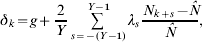
where
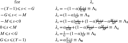
Note that λs is a piecewise linear function of the period s.
We can calculate that
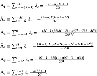
In addition, we have that  . Thus, we can derive that

For a constantly growing population, we have N t+1=(1+n)N 0. In this case, the dependency ratio (3) can be approximated as  . In a stationary state, this is constant at
 and thus
 . We can use this expression together with
 and the formulas (1), (2), (9), and (10) in the expression for the IRR ((12)). Linearizing the resulting expression around n=0 gives δk=g+n.
B.2 Relation of the internal rate of return to the implicit tax rate
The implicit tax is defined as the difference between the present value of pension benefits and the present value of contributions divided by the life-time income earned by a specific generation. In formal terms one can write

where ρ stands for the discount rate. Under the condition that this discount rate is equal to the growth rate of the economy (that is ρ=g) and using (4) we can simplify (23) to

This expression is in fact fairly similar to (13). We can now use the same steps as in B.1 to express ITR k as a linear function of cohort size N k+s. Note that one can write  , where A and B are defined as in B.1 and where C−D=G. Again it holds that
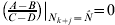 and thus

The main difference to the calculation of the IRR is that there 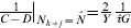 , while here
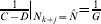 . Therefore
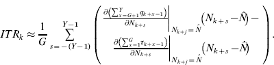
The rest of the calculation is exactly the same as in B.1 and the final expression for ITRk is also parallel
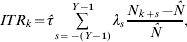
where the λs are defined as in B.1. For a stationary demographic situation with  , the implicit tax rate is thus zero for all generations. Otherwise, the implicit tax rate depends on the general size of the PAYG system (as measured by
 ) and on the exact development of cohort sizes. The pattern of the ITR for different generations can be inferred from Figure 1 (by multiplying λs with ).
B.3 Proposition 2
Part (i) We can derive from the expression for Λ1 to Λ6 that
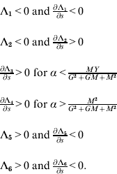
So all λs<−M are negative (and  ) and all λs>M are positive (and
 ). Since
 and
 are linear in s with exactly one extreme value, we can conclude that for each α there exists exactly one
 in
 for which
 .
Parts (ii) and (iii). The result follows from setting Λ3=0 (or equivalently Λ4=0) and solving for α. From this it also follows immediately that  . For
 , we can derive that
 and
 . Similarly, for
 we get that
 and
 . Since our model is formulated in discrete time, the
 should be understood as integer values of the respective formulas. Finally, we have that
 and
 .
B.4 Proposition 3
We use the fact (from proposition 1) that  , where the sums of positive and negative elasticities λ+ and λ− are defined as
 for λs>0 and
 for λs<0, respectively. Therefore,
 . The sum λ+ can be calculated for the two subintervals. For
 , we have that λ+=
 . It comes out as
 . For
 , we have that
 . It comes out as
 . For
 , we can calculate that
 . Furthermore, it holds that
 . From this it follows that λ+ is smallest for
 .
B.5 Proposition 4
The term  can be calculated as

Solving  for α gives the parameter αMinVar, where the variance of the IRR is at a minimum (if the second derivative is positive, which we have checked numerically). It comes out as the expression in (15).
 , q tR t=
 [(1−α)R t+αẑL t], and that
 (from (
 . This would not be necessary in the continuous time version of the model.
 ) as:
 .