A. Data

We estimate the U.S. term structure models using the zero-coupon yield data constructed by Gürkaynak et al. (Reference Gürkaynak, Sack and Wright2007) (GSW), available for download at the Federal Reserve Board’s website. The data set provides Nelson–Siegel–Svensson parameters. We use these parameters to back out the yields for maturities from 3 months to 10 years with a monthly increment. The data coverage goes back to June 14, 1961, which is the earliest starting point for the samples we study, matching the starting date of the ACM 10-year term premium provided by the Federal Reserve Bank of New York’s website.Footnote ³

We also estimate international yield curves using the updated Du, Im, and Schreger (Reference Du, Im and Schreger2018) data, which is originally from Bloomberg. The Bloomberg sample periods differ across countries, but all start after 1990. For Canada and the United Kingdom, the respective central banks provide longer yield curve data than Bloomberg, so we adopt the central banks’ data.

B. Estimation

We use the regression method of Adrian et al. (Reference Adrian, Crump and Moench2013) (ACM) to estimate both models. The method assumes that the state vector is observable and proceeds in two steps:

1. 1. Let $ {X}_t $ be the first five PCs of the yield curve. Estimate $ \boldsymbol{\mu}, \Phi, \Omega $ from equation (1) using OLS.

2. 2. Estimate $ {\Lambda}_0,{\Lambda}_1 $ from the excess bond return regression.

The regression is based on excess monthly holding period returns for maturities from 6 months to 5 years with a half-year increment, 7 years, and 10 years. The estimation of the FE model exactly follows the procedures in ACM.

For the FE model, the excess holding period return over one period is

(13) $$ {rx}_{t+1}^{(n)}={\mathcal{B}}_{n-1}^{\top}\left({\Lambda}_0-\boldsymbol{\mu} \right)-\frac{1}{2}{\mathcal{B}}_{n-1}^{\top}\Omega {\mathcal{B}}_{n-1}+{\mathcal{B}}_{n-1}^{\top}\left({\Lambda}_1-\Phi \right){X}_t+{\mathcal{B}}_{n-1}^{\top }{X}_{t+1}. $$

We add pricing errors to the excess bond returns as in ACM. The coefficients $ {\Lambda}_0 $ and $ {\Lambda}_1 $ can be backed out from regression coefficients of equation (13), which is estimated by regressing $ {rx}_{t+1}^{(n)} $ on $ {X}_t $ and $ {X}_{t+1} $ .

A. Summary Statistics

Interest rates are highly persistent. Since 1961, U.S. Treasury yields have increased steadily until 1981 and then declined almost monotonically until 2020. Between 1961 and 1981, Treasury yields rose by 10 percentage points, while from 1981 to 2020, they declined by more than 10 percentage points. The substantial changes in the yields make statistical analyses during this period highly sensitive to the choice of subsamples.

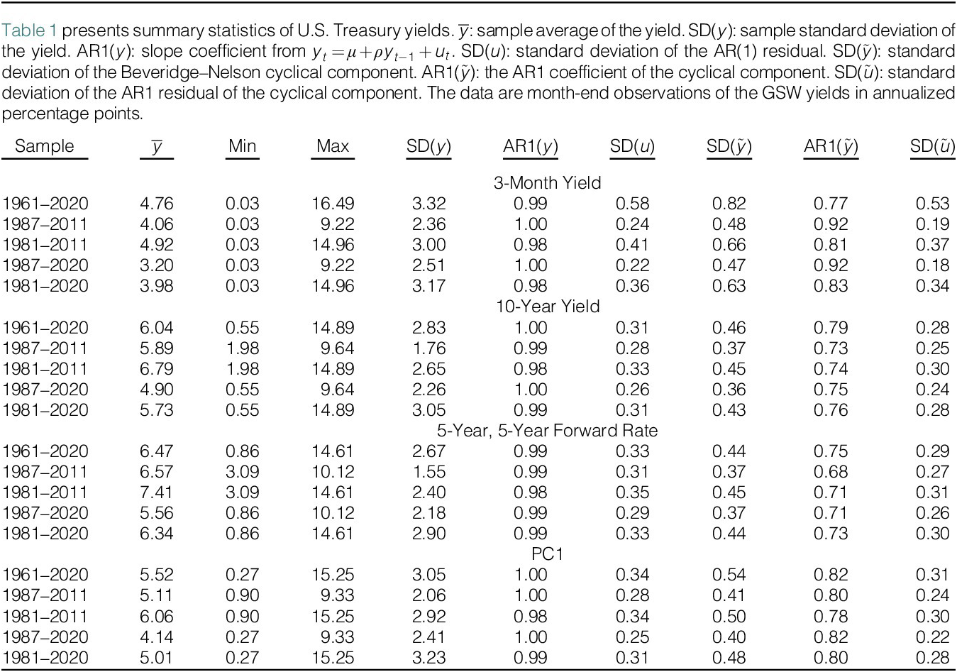
Table 1 presents the mean values ( $ \overline{y} $ ), minimum and maximum values, persistence and standard deviations of the 3-month yield, 10-year yield, 5-5 forward rate, and the first principal component 1 (PC1) of the monthly yield curve across various subsamples. Given that observed Treasury yields exhibit a single peak in 1981 during the 1961–2020 period, the average subsample yield tends to be higher when the subsample is closer to 1981. For instance, the average value of PC1 is 5.11% for the Adrian et al. (Reference Adrian, Crump and Moench2013) sample (1987–2011) but increases by nearly 1 percentage point to 6.06% when the starting date extends back to 1981. Another important statistic for the term structure model is the AR(1) coefficient, governing the rate of decay for the loading on $ {X}_t $ in equation (12). Treasury yields across all maturities are highly persistent, with AR(1) coefficients estimated across all subsamples being indistinguishable from 1. This indicates that the persistence of yield levels does not significantly contribute to the differences in estimated risk-neutral rates.

TABLE 1Summary Statistics of Treasury Yields

TABLE 1 Long description

The table contains 10 columns: Sample, y-bar (average yield), Min, Max, S D (y), A R 1 (y), S D (u), S D (y-tilde), A R 1 (y-tilde), and S D (u-tilde). Values are in annualized percentage points.

* 3-month yield section: For the full 1961 to 2020 sample, the average yield is 4.76 with a max of 16.49 and a min of 0.03. The A R 1 coefficient is 0.99.

* 10-year yield section: For the full 1961 to 2020 sample, the average yield is 6.04 with a max of 14.89 and a min of 0.55. The A R 1 coefficient is 1.00.

* 5-5 forward rate section: For the full 1961 to 2020 sample, the average yield is 6.47 with a max of 14.61 and a min of 0.86. The A R 1 coefficient is 0.99.

* P C 1 section: For the full 1961 to 2020 sample, the average yield is 5.52 with a max of 15.25 and a min of 0.27. The A R 1 coefficient is 1.00.

Across all categories, the 1981 to 2011 period consistently shows the highest average yields (e.g., 7.41 for the 5-5 forward rate) and the highest maximums. The A R 1 (y) values remain extremely high across all samples, ranging from 0.98 to 1.00, indicating high persistence in the yields.

B. Estimated Risk-Neutral Rates

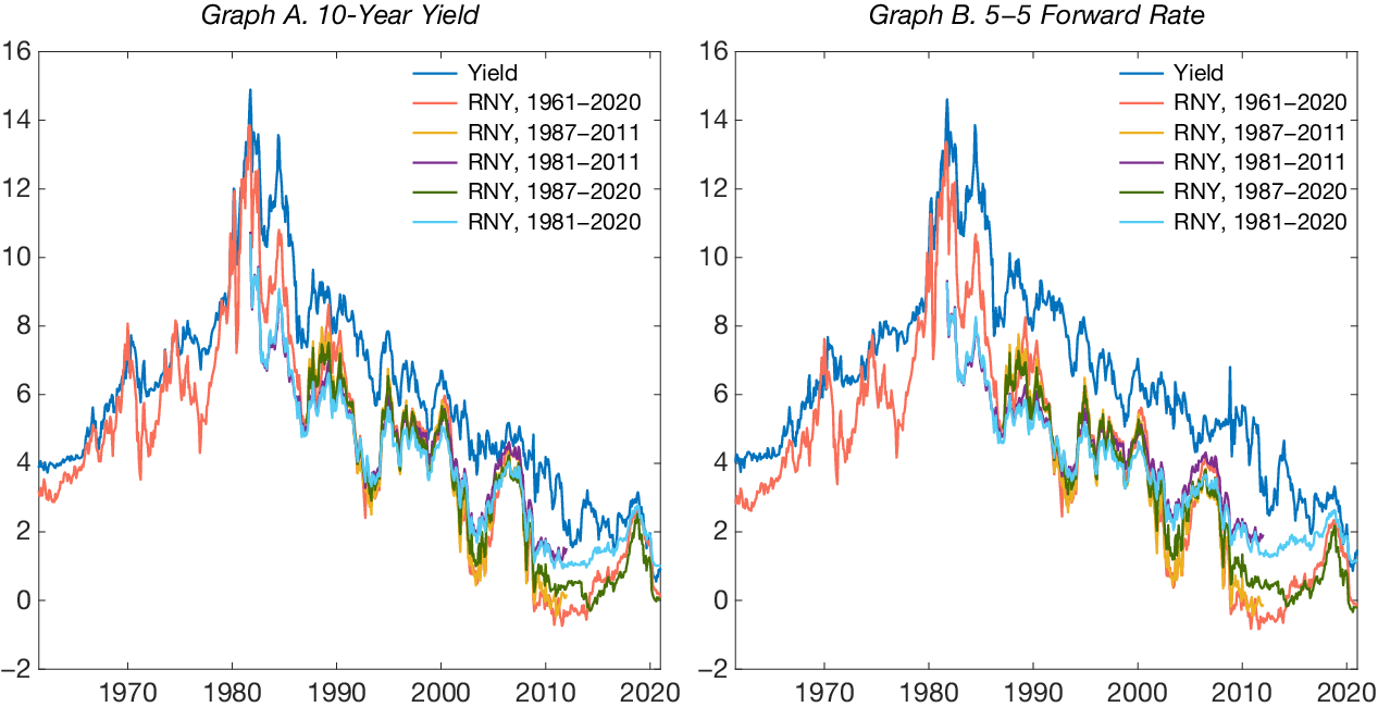
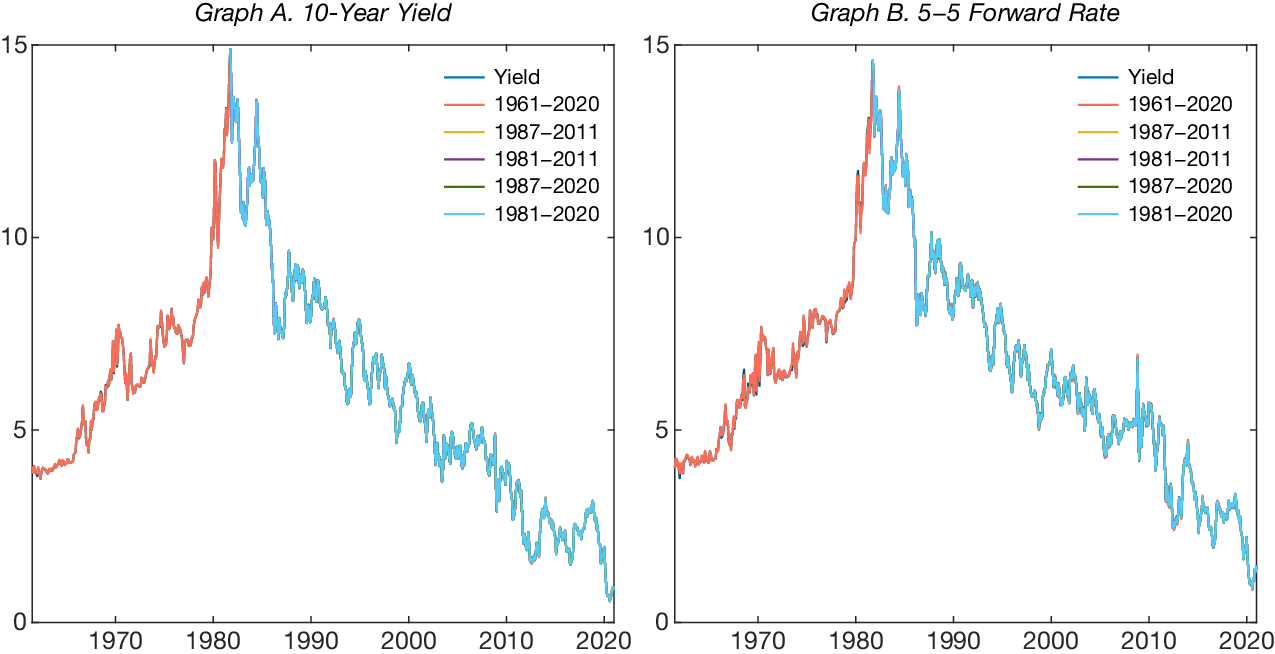
Figure 1 presents the time series of the 10-year yield (Graph A) and the 5-5 forward rates (Graph B) together with their risk-neutral components estimated using different sample periods. A striking feature is that the estimated risk-neutral rates do not coincide during the overlapping sample periods, although they should. For instance, the 10-year risk-neutral rate for January 1990 is estimated at 6.46% using the 1961–2020 sample, 4.89% using the 1987–2011 sample, and 4.23% using the 1981–2020 sample. This variation in estimates illustrates a substantial change of 52% ((6.46–4.23)/4.23). The discrepancy is even more pronounced for the 5-5 forward rate. For September 1981, the estimated risk-neutral rate is 9.29% using the 1961–2020 sample, compared to 4.70% using the 1981–2011 sample. This results in a difference of 4.6 percentage points, or an astounding 98% ((9.29–4.70)/4.70)!

FIGURE 1ACM Risk-Neutral Yields Estimated on Different Samples

In Figure 1, the risk-neutral yields are estimated from the canonical Adrian et al. (Reference Adrian, Crump and Moench2013) model using different sample periods. The “Yield” series are the observed yields.

FIGURE 1 Long description

A two-panel line graph. Both panels share a vertical Y axis ranging from 0 to 15 and a horizontal X axis representing years from 1961 to 2020.

Graph A, titled 10-Year Yield, shows six data series. The dark teal line representing Yield is the most volatile, peaking near 15 in the early 1980s before trending downward. Five R N Y (Risk-Neutral Yield) lines follow a similar but smoother trajectory. The R N Y 1961-2020 (orange) spans the full duration. Shorter series including R N Y 1987-2011 (yellow), R N Y 1981-2011 (purple), R N Y 1987-2020 (green), and R N Y 1981-2020 (light blue) begin at their respective start dates and generally cluster below the actual Yield line after 1985.

Graph B, titled 5-5 Forward Rate, displays the same six categories. The dark teal Yield line again shows the highest peaks and most significant volatility. The R N Y series in this panel are more tightly grouped together than in Graph A, particularly from 1990 onwards, where they show a consistent downward trend toward 2 percent by 2020. The green line (R N Y 1987-2020) shows the lowest values in the final decade, dipping toward 0 around 2015.

The risk-neutral rates estimated using different sample periods do not merely differ by constants, that is, they are not parallel shifts of each other. For instance, the risk-neutral rates estimated using the 1981–2020 sample are flatter than those from other sample periods and exhibit less cyclical fluctuation. This indicates that the loadings of the risk-neutral rates on the state variables, $ {\mathcal{B}}_n^{rn} $ from equation (10), are highly sensitive to the choice of sample periods. As a result, the estimated responses of risk-neutral rates to shocks can be unreliable and strongly influenced by the sample period chosen for estimating the risk-neutral rates, even when the sample for estimating impulse responses is fixed. In Section V, we present an example demonstrating that the responses of risk-neutral rates to monetary policy shocks can differ by more than fourfold, depending on whether the risk-neutral rates are estimated using the post-1961 or the post-1987 sample.

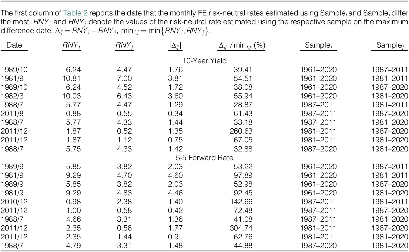
To quantify the differences in the risk-neutral rates illustrated in the figure, we compute the maximum difference between the risk-neutral rates estimated using pairs of sample periods. According to Table 2, the 10-year risk-neutral rates estimated for a given date can differ by as much as 3.81 percentage points. Similarly, the 5-5 risk-neutral forward rate can vary by 4.60 percentage points. In relative terms, this difference represents at least 29% of the lower estimate for the 10-year risk-neutral rate and 41% for the 5-5 risk-neutral forward rate.

TABLE 2Maximum Difference in Risk-Neutral Rates Estimated from Different Samples

TABLE 2 Long description

The table consists of seven columns: Date, R N Y sub i, R N Y sub j, absolute Delta sub i j, absolute Delta sub i j all over min sub i comma j (percentage), Sample i, and Sample j. It is divided into two horizontal sections.

10-year yield section:

* Row 1: 1989/10, 6.24, 4.47, 1.76, 39.41, 1961–2020, 1987–2011.

* Row 2: 1981/9, 10.81, 7.00, 3.81, 54.51, 1961–2020, 1981–2011.

* Row 3: 1989/10, 6.24, 4.52, 1.72, 38.08, 1961–2020, 1987–2020.

* Row 4: 1982/3, 10.03, 6.43, 3.60, 55.94, 1961–2020, 1981–2020.

* Row 5: 1988/7, 5.77, 4.47, 1.29, 28.87, 1987–2011, 1981–2011.

* Row 6: 2011/8, 0.88, 0.55, 0.34, 61.43, 1987–2011, 1987–2020.

* Row 7: 1988/7, 5.77, 4.33, 1.44, 33.18, 1987–2011, 1981–2020.

* Row 8: 2011/12, 1.87, 0.52, 1.35, 260.63, 1981–2011, 1987–2020.

* Row 9: 2011/12, 1.87, 1.12, 0.75, 67.05, 1981–2011, 1981–2020.

* Row 10: 1988/7, 5.75, 4.33, 1.42, 32.88, 1987–2020, 1981–2020.

5-5 forward rate section:

* Row 1: 1989/9, 5.85, 3.82, 2.03, 53.22, 1961–2020, 1987–2011.

* Row 2: 1981/9, 9.29, 4.70, 4.60, 97.89, 1961–2020, 1981–2011.

* Row 3: 1989/9, 5.85, 3.82, 2.03, 52.98, 1961–2020, 1987–2020.

* Row 4: 1981/9, 9.29, 4.83, 4.46, 92.45, 1961–2020, 1981–2020.

* Row 5: 2010/12, 0.98, 2.38, 1.40, 142.66, 1987–2011, 1981–2011.

* Row 6: 2011/12, 1.00, 0.58, 0.42, 72.48, 1987–2011, 1987–2020.

* Row 7: 1988/7, 4.66, 3.31, 1.36, 41.08, 1987–2011, 1981–2020.

* Row 8: 2011/12, 2.35, 0.58, 1.77, 304.74, 1981–2011, 1987–2020.

* Row 9: 2011/12, 2.35, 1.44, 0.91, 62.76, 1981–2011, 1981–2020.

* Row 10: 1988/7, 4.79, 3.31, 1.48, 44.88, 1987–2020, 1981–2020.

C. Bias Correction

A potential issue in estimating the term structure model is that the OLS estimator may underestimate the persistence of the state vector $ {X}_t $ in the first step of the ACM algorithm. This problem is particularly severe when the sample size is small. Since the loadings of the risk-neutral rates on $ {X}_t $ depend on the persistence matrix $ \Phi $ , this bias could contribute to the inconsistencies observed in this section. Bauer et al. (Reference Bauer, Rudebusch and Wu2012) (BRW) propose a bias-correction method based on simulations to make the estimated $ \hat{\Phi} $ more persistent than the OLS result.

In Step 1, we estimate $ \boldsymbol{\mu}, \Phi, \Omega $ using the bias-correction method instead of the standard OLS method. Given the estimated $ \boldsymbol{\mu}, \Phi, \Omega $ , we proceed to Step 2 as in Section III.B.

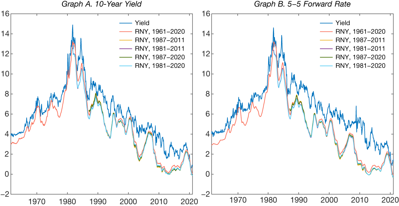
Figure 2 presents the bias-corrected ACM risk-neutral rates estimated from different sample periods. Compared with the uncorrected estimates in Figure 1, the risk-neutral rates appear to be higher, especially for those estimated using post-1981 samples. The risk-neutral rates estimated using the post-1981 samples are closer to those estimated using the 1961–2020 sample. However, there are still substantial inconsistencies in the 1980s, early 2000s, and 2010s.

FIGURE 2ACM Bias-Corrected Risk-Neutral Yields Estimated on Different Samples

In Figure 2, the risk-neutral yields are estimated from the canonical Adrian et al. (Reference Adrian, Crump and Moench2013) model, where the VAR parameters are bias-corrected using the method of Bauer et al. (Reference Bauer, Rudebusch and Wu2012). The “Yield” series are the observed yields.

FIGURE 2 Long description

A two-panel line graph. Both panels share a horizontal x-axis representing years from 1961 to 2020 and a vertical y-axis representing percentage rates from negative 2 to 16.

Graph A, titled 10-Year Yield, shows a dark blue line for Yield and five colored lines for R N Y (Risk-Neutral Yield) based on different sample periods. The Yield line peaks near 15 percent in the early 1980s before trending downward to near 1 percent by 2020. The R N Y lines generally follow the Yield trend but remain lower, particularly after 1990. The R N Y 1961-2020 (orange) and R N Y 1981-2020 (light blue) show the highest estimates among the risk-neutral models, while R N Y 1987-2011 (yellow) and R N Y 1981-2011 (purple) show the lowest, dipping near 0 percent after 2010.

Graph B, titled 5-5 Forward Rate, displays a similar structure. The Yield line (dark blue) peaks at approximately 14 percent in the early 1980s and declines to roughly 2 percent by 2020. The R N Y lines show a more pronounced divergence from the actual Yield than in Graph A. Specifically, after 2010, the R N Y 1961-2020 (orange) and R N Y 1987-2011 (yellow) drop below 0 percent, while the R N Y 1981-2020 (light blue) remains higher, around 2 percent.

A. High-Frequency Regressions

A standard approach to estimating the effects of monetary policy shocks involves regressing the dependent variable on the shock. We estimate the following equation:

(14) $$ \Delta {y}_t={\beta}_0+{\beta}_1{x}_t+{\varepsilon}_t, $$

where each $ t $ corresponds to an FOMC monetary policy announcement. Here, $ \Delta {y}_t $ is the daily change in a Treasury yield or its risk-neutral component on the announcement day, and $ {x}_t $ denotes a measure of the monetary policy shock. A standard measure of the monetary policy shock is the change in the Eurodollar futures rates, with maturities ranging from the current quarter to a year ahead, during 30-minute event windows bracketing monetary policy announcements. We summarize the Eurodollar shocks with the first PC, denoted as $ {MPS}_t $ . Furthermore, Bauer and Swanson (Reference Bauer, Swanson, Eichenbaum, Hurst and Ramey2022), (Reference Bauer and Swanson2023) argue that $ {MPS}_t $ contains a component that responds to macroeconomic news and is not fully exogenous to information before the FOMC meeting. They extract a component $ {MPS}_t^o $ from $ {MPS}_t $ that is orthogonal to macroeconomic news, which we also consider in our regression. FOMC announcements not only set the current target for the federal funds rate but also convey information about its future path. The latter is especially relevant for long-maturity yields because the expected path of the short-term interest rate (risk-neutral yield) is an important component of long-maturity yields. Following Gürkaynak et al. (Reference Gürkaynak, Sack and Swanson2005), we use their target and path factors to measure shocks to the current federal funds rate target and the expected policy rates, respectively.

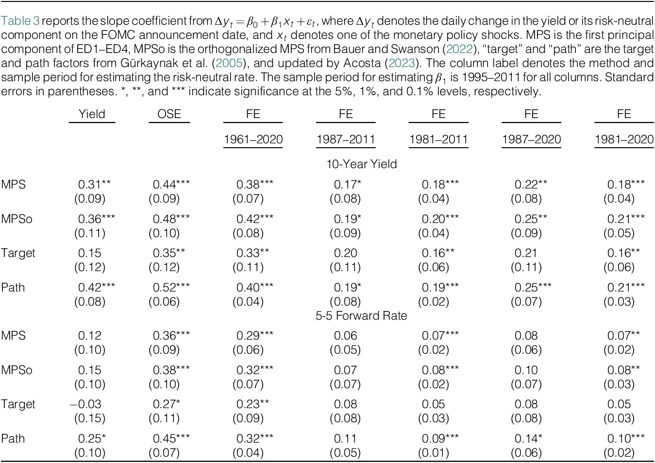
Table 3 reports the estimated responses of the 10-year yield and the 5-5 forward rate and their risk-neutral components to various measures of the monetary policy shock. We estimate the ACM risk-neutral rate parameters using the sample periods considered in Figure 1. Then, we combine the respective monthly model parameters with daily yield curve PCs to compute daily risk-neutral rates for the regression analysis. The regression sample period is from 1995 to 2011, which is the maximal intersection among all monetary policy shock data and the risk-neutral rate estimation samples.

TABLE 3Contemporaneous Effects of Monetary Policy Shocks

TABLE 3 Long description

The table reports slope coefficients (beta sub 1) from regressions of daily changes in yields on monetary policy shocks.

Header Structure:

* Column 1: Yield (raw data).

* Column 2: O S E.

* Columns 3 to 7: F E (Fixed Effects) with varying sample periods: 1961–2020, 1987–2011, 1981–2011, 1987–2020, and 1981–2020.

Section 1: 10-year yield

* M P S: Coefficients range from 0.17 to 0.44, with standard errors between 0.04 and 0.09. Most are significant at the 0.1% or 1% level.

* M P S o: Coefficients range from 0.19 to 0.48, showing slightly higher sensitivity than M P S.

* Target: Coefficients range from 0.15 to 0.35; significance is lower compared to other shocks.

* Path: Coefficients range from 0.19 to 0.52, highly significant across most columns.

Section 2: 5-5 forward rate

* M P S: Coefficients range from 0.06 to 0.36. Significance is primarily found in O S E and specific F E models.

* M P S o: Coefficients range from 0.07 to 0.38.

* Target: Coefficients range from -0.03 to 0.27, with many being statistically insignificant.

* Path: Coefficients range from 0.09 to 0.45, showing the strongest and most consistent significance in this section.

Standard errors are provided in parentheses below each coefficient. Asterisks indicate significance levels: * for 5%, ** for 1%, and *** for 0.1%.

Monetary policy shocks significantly affect long-maturity yields. For example, when $ {MPS}_t $ decreases by 1 percentage point, the 10-year yield decreases by 33 basis points. The path factor has much stronger effects on long-maturity yields than the target factor, which is intuitive. How much of the effects are due to the responses of expected short-term rates? According to the ACM model estimated using 1961–2020 data, the risk-neutral rates respond much more strongly than the term premia to monetary policy shocks.Footnote ⁴ However, the same model estimated using post-1981 data suggests that the expectations hypothesis component of the 10-year yield is less than half as responsive to monetary policy shocks as the model using 1961–2020 data suggests. More starkly, the 5-5 forward rate results differ by a factor of more than three.

B. Bias-Corrected Risk-Neutral Rates

To examine whether bias correction alleviates the inconsistency problem in high-frequency regressions, we re-estimate equation (14) using BRW bias-corrected risk-neutral yields as the dependent variable. Albagli et al. (Reference Albagli, Ceballos, Claro and Romero2019) use a similar method to estimate the risk-neutral yields and study the effects of U.S. monetary policy shocks on world long-term yields.

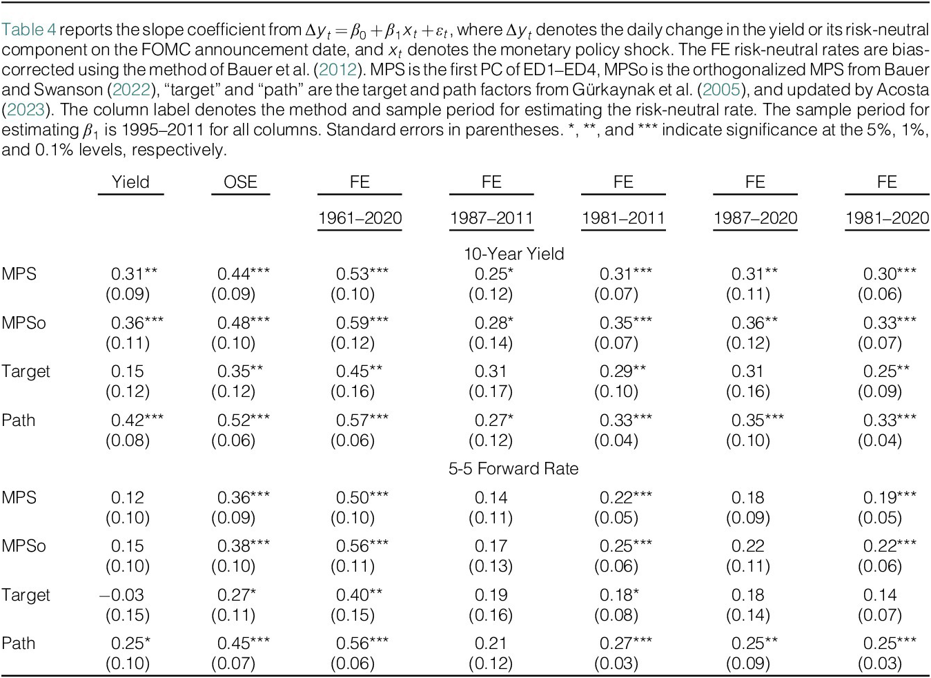
Table 4 reports the estimated effects of high-frequency monetary policy shocks on bias-corrected risk-neutral yields, where the risk-neutral yields are estimated using the same sample periods as in Table 3, and the regressions are estimated using the 1995–2011 sample. Compared with the results in Table 3, the bias-corrected risk-neutral yields are more responsive to monetary policy shocks regardless of the sample periods for estimating the term structure model. However, the bias correction does not make the estimated $ {\hat{\beta}}_1 $ more consistent across sample periods. For example, the 10-year risk-neutral yield estimated from the 1961–2020 sample is twice as responsive to monetary policy shocks as the one estimated from the 1987–2011 sample.

TABLE 4Contemporaneous Effects of Monetary Policy Shocks: Bias-Corrected Risk-Neutral Rates

TABLE 4 Long description

The table is divided into two main vertical sections: 10-year yield and 5-5 forward rate. The columns represent different estimation methods: Yield, O S E, and five variations of F E with different sample periods (1961–2020, 1987–2011, 1981–2011, 1987–2020, and 1981–2020). The rows represent four types of monetary policy shocks: M P S, M P S o, Target, and Path.

In the 10-year yield section:

* M P S coefficients range from 0.25 to 0.53, with standard errors between 0.06 and 0.12.

* M P S o coefficients range from 0.28 to 0.59, with standard errors between 0.07 and 0.14.

* Target coefficients range from 0.15 to 0.45, with standard errors between 0.09 and 0.17.

* Path coefficients range from 0.27 to 0.57, with standard errors between 0.04 and 0.12.

In the 5-5 forward rate section:

* M P S coefficients range from 0.12 to 0.50, with standard errors between 0.05 and 0.11.

* M P S o coefficients range from 0.15 to 0.56, with standard errors between 0.06 and 0.13.

* Target coefficients range from -0.03 to 0.40, with standard errors between 0.07 and 0.16.

* Path coefficients range from 0.21 to 0.56, with standard errors between 0.03 and 0.12.

Asterisks indicate statistical significance: * for 5 percent, ** for 1 percent, and *** for 0.1 percent levels. Standard errors are provided in parentheses below each coefficient.

A. A Shifting Endpoint Model

The same state vector $ {X}_t $ as in the FE model determines the yield curve. However, we now assume that $ {X}_t $ contains a random walk component

(15) $$ {\displaystyle \begin{array}{l}{X}_t=\boldsymbol{\mu} +\Gamma {\boldsymbol{\tau}}_t+{\tilde{X}}_t,\\ {}{\boldsymbol{\tau}}_t={\boldsymbol{\tau}}_{t-1}+{\boldsymbol{\eta}}_t,\hskip1em {\boldsymbol{\eta}}_t\sim \mathcal{N}\left(0,{\Omega}_{\eta}\right)\\ {}{\tilde{X}}_t=\Phi {\tilde{X}}_{t-1}+{\tilde{U}}_t,\hskip1em {\tilde{U}}_t\sim \mathcal{N}\left(0,\tilde{\Omega}\right),\end{array}} $$

where $ {\boldsymbol{\tau}}_t $ is a $ {K}_{\tau}\times 1 $ random walk and $ {\tilde{X}}_t $ is a $ K\times 1 $ stationary VAR(1). The shocks are IID (independent and identically distributed) over time and $ {\boldsymbol{\eta}}_t\perp {\tilde{U}}_t $ . Define

$$ {Z}_t\equiv {\left[{\boldsymbol{\tau}}_t^{\top}\hskip0.5em {X}_t^{\top}\right]}^{\top },{U}_t\equiv \Gamma {\boldsymbol{\eta}}_t+{\tilde{U}}_t,\Omega \equiv \mathbf{E}\left[{U}_t{U}_t^{\top}\right]={\Gamma \Omega}_{\eta }{\Gamma}^{\top }+\tilde{\Omega}. $$

The SDF is exponentially affine:

(16) $$ \ln {M}_{t,t+1}=-{\delta}_0-{\boldsymbol{\delta}}_1^{\top }{X}_t-\frac{1}{2}{\Lambda}_t^{\top }{\Lambda}_t-{\Lambda}_t^{\top }{\Omega}^{-\frac{1}{2}}{U}_{t+1}. $$

The price of risk is an affine function of $ {Z}_t $ :

(17) $$ {\Lambda}_t={\Sigma}^{-1}\left({\Lambda}_0+{\Lambda}_1{Z}_t\right), $$

where $ {\Sigma \Sigma}^{\top }=\Omega $ .

Note that the log SDF is affine in $ {X}_t $ , but the market prices of risk are affine in $ {Z}_t $ . The shock $ {U}_{t+1} $ is a $ K\times 1 $ dimensional vector with the same dimension as $ {X}_t $ but is a combination of shocks to $ {\boldsymbol{\tau}}_t $ and $ {\tilde{X}}_t $ . We assume that $ {\Lambda}_1 $ satisfies

(18) $$ {\Lambda}_1=\left[\begin{array}{c}\left(I-\Phi \right)\Gamma, {\Lambda}_{12}\end{array}\right], $$

that is, the first $ {K}_{\tau } $ column of $ {\Lambda}_1 $ (the loading on $ {\boldsymbol{\tau}}_t $ ) equals $ \left(I-\Phi \right)\Gamma $ and the remaining $ K $ columns are an unrestricted $ K\times K $ matrix $ {\Lambda}_{12} $ . This implies that the log bond prices are still affine in $ {X}_t $ , taking the same form as equation (6). Although the trend $ {\boldsymbol{\tau}}_{\mathbf{t}} $ does not directly affect the observed yields, it affects term premia by affecting the price of risk, so the risk-neutral bond prices are

(19) $$ \ln {P}_t^{(n) rn}={\mathcal{A}}_n^{rn}+{\mathcal{B}}_n^{rn\top }{X}_t+{\mathcal{C}}_n^{rn\top }{\boldsymbol{\tau}}_t. $$

The risk-neutral parameters solve the following recursions:

(20) $$ {\displaystyle \begin{array}{l}{\mathcal{A}}_n^{rn}={\mathcal{A}}_{n-1}^{rn}-{\delta}_0+{\mathcal{B}}_{n-1}^{rn\top}\left(I-\Phi \right)\boldsymbol{\mu} +\frac{1}{2}{\mathcal{B}}_{n-1}^{rn\top}\Omega {\mathcal{B}}_{n-1}^{rn},\\ {}+\frac{1}{2}\left({\mathcal{B}}_{n-1}^{rn\top }{\Gamma \Omega}_{\eta }{\mathcal{C}}_{n-1}^{rn}+{\mathcal{C}}_{n-1}^{rn\top }{\Omega}_{\eta }{\Gamma}^{\top }{\mathcal{B}}_{n-1}\right)+\frac{1}{2}{\mathcal{C}}_{n-1}^{rn\top }{\Omega}_{\eta }{\mathcal{C}}_{n-1}^{rn},\hskip1em {\mathcal{A}}_1=-{\delta}_0,\end{array}} $$

(21) $$ {\mathcal{B}}_n^{rn\top }={\mathcal{B}}_{n-1}^{rn\top}\Phi -{\boldsymbol{\delta}}_1^{\top },\hskip1em {\mathcal{B}}_1=-{\boldsymbol{\delta}}_1, $$

(22) $$ {\mathcal{C}}_n^{rn\top }={\mathcal{B}}_{n-1}^{rn\top}\left(I-\Phi \right)\Gamma +{\mathcal{C}}_{n-1}^{rn\top },\hskip1em {\mathcal{C}}_1=\mathbf{0}. $$

B. Estimation

We follow similar estimation procedures as the FE model. The excess holding period return over one period for the shifting endpoint model is

(23) $$ {rx}_{t+1}^{(n)}={\mathcal{B}}_{n-1}^{\top}\left({\Lambda}_0-\left(I-\Phi \right)\boldsymbol{\mu} \right)-\frac{1}{2}{\mathcal{B}}_{n-1}^{\top}\Omega {\mathcal{B}}_{n-1}+{\mathcal{B}}_{n-1}^{\top}\left({\Lambda}_{12}-\Phi \right){X}_t+{\mathcal{B}}_{n-1}^{\top }{X}_{t+1}. $$

Note that $ \Phi $ here refers to the persistence parameter of the cyclical component $ {\tilde{X}}_t $ of the state vector, whereas the $ \Phi $ in equation (13) refers to the persistence parameter of the state vector $ {X}_t $ . This is the main reason that the two models produce different estimates of the risk-neutral rates.

A prerequisite for estimating the risk-neutral rates is to obtain a $ {\tau}_t $ series. For the monthly model, we estimate $ {\tau}_t $ as the Beveridge–Nelson trend of the first PC of the yield curve using the method of Kamber, Morley, and Wong (Reference Kamber, Morley and Wong2018), (Reference Kamber, Morley and Wong2025). Alternatively, we can estimate equation (15) using the Bayesian method as in Bauer and Rudebusch (Reference Bauer and Rudebusch2020) and Del Negro, Giannone, Giannoni, and Tambalotti (Reference Del Negro, Giannone, Giannoni, Tambalotti, Eberly and Stock2017). The two methods produce virtually identical results, but our method is much faster.Footnote ⁵ Since $ {\tau}_t $ is estimated, we refer to this method as the “estimated shifting endpoint” (ESE) model, following Bauer and Rudebusch (Reference Bauer and Rudebusch2020). The state variables $ {X}_t,{\tau}_t $ and the model parameters $ \mathcal{A},\mathcal{B},{\mathcal{A}}^{rn},{\mathcal{B}}^{rn},{\mathcal{C}}^{rn} $ are estimated using data from each subsample. At the daily frequency, the estimation of $ {\tau}_t $ becomes unreliable. Instead, we proxy $ {\tau}_t $ with the first PC of the sum of daily changes in Treasury yields during three-day windows bracketing FOMC announcements. Hillenbrand (Reference Hillenbrand2025) shows that the series explains the persistent variations in Treasury yields almost perfectly, making it a suitable proxy for $ {\tau}_t $ in the shifting endpoint model. We denote this method as the “observed shifting endpoint” (OSE) model.Footnote ⁶

C. ESE Risk-Neutral Rates

Figure 3 presents the monthly 10-year yield (Graph A) and the 5-5 forward rate (Graph B) alongside their ESE risk-neutral components, estimated using the same sample periods as in Figure 1. Notably, the risk-neutral components for a given yield estimated with different samples almost coincide, effectively addressing the discrepancy problem associated with the FE model. Furthermore, the risk-neutral rates implied by the ESE model are higher than those implied by the FE model and are more parallel to the observed yields.

FIGURE 3ESE Risk-Neutral Yields Estimated on Different Samples

In Figure 3, the risk-neutral yields are estimated from the ESE model using different sample periods. The “Yield” series are the observed yields.

FIGURE 3 Long description

Two side-by-side line graphs. Both share a vertical Y axis ranging from minus 2 to 16 and a horizontal X axis representing years from 1970 to 2020.

Graph A, titled 10-Year Yield, displays a dark teal line for actual Yield and five colored lines for R N Y (Risk-Neutral Yield) estimates based on different sample periods: 1961-2020 (orange), 1987-2011 (yellow), 1981-2011 (purple), 1987-2020 (green), and 1981-2020 (light blue). All lines show a sharp climb from 1970, peaking around 1981 at approximately 15 percent, followed by a long-term stochastic decline toward 0 percent by 2020. The actual Yield line remains consistently higher than the R N Y estimates after 1985.

Graph B, titled 5-5 Forward Rate, follows a nearly identical trajectory and color scheme. The actual Yield (dark teal) shows higher volatility and remains elevated above the clustered R N Y estimates from the mid-1980s onward. In both graphs, the various R N Y estimates (1987-2011, 1981-2011, 1987-2020, and 1981-2020) are tightly grouped, while the 1961-2020 estimate occasionally diverges slightly higher during the 1970s.

A. Contemporaneous Effects

We revisit the high-frequency regression equation (14) using OSE risk-neutral yields. Since the empirical proxy for $ {\tau}_t $ is only available after 1989, we consider two sample periods for estimating the term structure model: 1989–2011 and 1989–2020. The sample period for estimating equation (14) is 1995–2011.

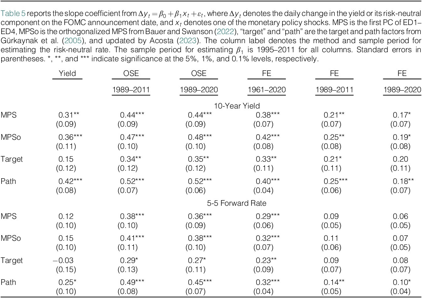
Table 5 reports the effects of high-frequency monetary policy shocks on OSE risk-neutral yields. To facilitate comparison, we reproduce the ACM FE risk-neutral yields using the 1989–2011 and 1989–2020 sample periods. The estimated $ {\hat{\beta}}_1 $ is much more stable across sample periods for the OSE risk-neutral yields than for the FE ones.

TABLE 5Contemporaneous Effects of Monetary Policy Shocks

TABLE 5 Long description

The table is structured with six columns of data under the headings Yield, O S E (1989–2011), O S E (1989–2020), F E (1961–2020), F E (1989–2011), and F E (1989–2020). It is divided into two horizontal sections.

Section 1: 10-year yield.

* M P S: Coefficients range from 0.17 to 0.44, with standard errors between 0.07 and 0.09.

* M P S o: Coefficients range from 0.19 to 0.48, with standard errors between 0.08 and 0.11.

* Target: Coefficients range from 0.15 to 0.35, with standard errors between 0.11 and 0.12.

* Path: Coefficients range from 0.18 to 0.52, with standard errors between 0.04 and 0.08.

Section 2: 5-5 forward rate.

* M P S: Coefficients range from 0.06 to 0.38, with standard errors between 0.05 and 0.10.

* M P S o: Coefficients range from 0.07 to 0.41, with standard errors between 0.05 and 0.11.

* Target: Coefficients range from -0.03 to 0.29, with standard errors between 0.07 and 0.15.

* Path: Coefficients range from 0.10 to 0.49, with standard errors between 0.04 and 0.10.

Statistical significance is indicated by asterisks: * for 5 percent, ** for 1 percent, and *** for 0.1 percent levels. Standard errors are provided in parentheses below each coefficient.

Interestingly, the OSE results are similar to the FE results estimated from the 1961–2020 sample, and the differences in $ {\hat{\beta}}_1 $ between the FE, 1961–2020 column and the FE, post-1989 columns are much larger than the difference between the FE, post-1989 columns. This further indicates that the high-frequency regression results are highly sensitive to the sample periods for estimating the FE term structure model, and the OSE method significantly stabilizes the estimation results.

B. Cumulative Effects of Monetary Policy Announcements

In an intriguing paper, Hillenbrand (Reference Hillenbrand2025) demonstrates that 3-day windows around FOMC announcements can almost perfectly explain the persistent variations in long-maturity Treasury yields since 1989. How much of this phenomenon is attributable to the expectations hypothesis component? We show that the answer to this question, according to the FE model, highly depends on the sample period used to estimate the risk-neutral rates.

To quantify the fraction of total variations in the FOMC-window changes explained by the expectations hypothesis component, we define the adjusted R-squared $ {\tilde{R}}^2 $ as follows:

(24) $$ {\tilde{R}}^2=1-\frac{\sum_t{\left({y}_t^{FOMC}-{y}_t^{rn, FOMC}\right)}^2}{\sum_t{\left({y}_t^{FOMC}-{y}_t^{rn, FOMC}\right)}^2+{\sum}_t{\left({y}_t^{FOMC}-{y}_t^{tp, FOMC}\right)}^2}. $$

In this equation, $ {y}_t^{FOMC} $ denotes the cumulative change in $ {y}_t $ during FOMC windows up to $ t $ , while $ {y}_t^{rn, FOMC} $ and $ {y}_t^{tp, FOMC} $ denote the cumulative changes in the risk-neutral and term premium components of $ {y}_t $ during FOMC windows up to $ t $ . Note that $ {y}_t^{rn, FOMC}+{y}_t^{tp, FOMC}={y}_t^{FOMC} $ , and $ {\tilde{R}}^2\in \left[0,1\right] $ . A bigger $ {\tilde{R}}^2 $ indicates that the risk-neutral component explains a larger fraction of the total variations in $ {y}_t^{FOMC} $ .

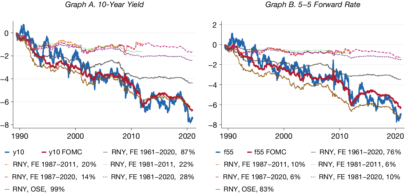
In Figure 4, we present the actual 10-year yield (Graph A) and the 5-5 forward rate (Graph B), along with their cumulative changes during FOMC windows and the cumulative changes in their risk-neutral components during these windows. When risk-neutral rates are estimated using the 1961–2020 sample or directly sourced from the Federal Reserve Bank of New York’s website, the expectations hypothesis explains 87% of the cumulative change in the 10-year yield and 76% of that in the 5-5 forward rate during the FOMC windows. In contrast, when risk-neutral rates are estimated using sample periods closely aligned with the FOMC sample, such as the 1987–2020 sample, the expectations hypothesis results in a significantly lower $ {\tilde{R}}^2 $ of only 14% for the 10-year yield and 6% for the 5-5 forward rate. However, utilizing the post-1989 sample with the OSE method indicates that the expectations hypothesis explains nearly all of the yield dynamics during the FOMC windows. The $ {\tilde{R}}^2 $ for this case is strikingly high at 99% for the 10-year yield and 83% for the 5–5 forward rate.

FIGURE 4Cumulative Change in the Risk-Neutral Rates During FOMC Windows

In Figure 4, the series y10 and f55 are the observed 10-year Treasury yield and 5-5 forward rate relative to their initial values, y10FOMC and f55FOMC are the sums of daily changes in y10 and f55 during FOMC windows, and the remaining series are cumulative changes in the risk-neutral rates from the OSE or FE model estimated on different samples. The percentage number indicates the fraction of total variation in y10FOMC or f55FOMC explained by the respective risk-neutral rate.

FIGURE 4 Long description

A two-panel line graph. Both panels share an x-axis ranging from 1990 to 2020 and a y-axis ranging from -8 to 2.

Graph A, titled 10-Year Yield, tracks y 10 and y 10 F O M C. The blue line y 10 shows high volatility, ending near -8. The thick red line y 10 F O M C follows a similar downward trend, ending near -7. Several thinner lines represent R N Y models. The R N Y O S E model in brown closely tracks the red line with 99 percent explanation. Other models like R N Y F E 1961-2020 in grey and various dashed lines for different year ranges stay higher on the y-axis, ending between -2 and -4.

Graph B, titled 5-5 Forward Rate, tracks f 55 and f 55 F O M C. The blue line f 55 and thick red line f 55 F O M C both trend downward to approximately -7. The R N Y O S E model in brown tracks the downward trend most closely at 83 percent. The R N Y F E 1961-2020 model in grey ends near -3.5, while other F E models for 1987-2011, 1981-2011, 1987-2020, and 1981-2020 cluster between -1 and -2.5 at the end of the period.

A. Consistency of Parameters

Why are the risk-neutral rates estimated from the FE model highly sensitive to sample periods? Table 1 suggests that the average yields differ substantially over time, so the estimate of $ \boldsymbol{\mu} $ is sensitive to the choice of sample periods. According to equation (11), differences in $ \boldsymbol{\mu} $ lead to differences in $ {\mathcal{A}}_n^{rn} $ , the intercept for risk-neutral rates. Consequently, the levels of risk-neutral rates estimated from different subsamples are different.

More interestingly, the risk-neutral rates estimated from different sample periods also exhibit different slopes and volatility of cyclical fluctuations, indicating differences in $ {\mathcal{B}}_n^{rn} $ . Figure 6A plots the FE model’s $ {\mathcal{B}}_n^{rn} $ against maturity $ n $ . Each graph of Figure 6A plots the coefficient on an element of $ {X}_t $ . For example, the point with a horizontal coordinate 50 in graph $ {\mathcal{B}}^{rn}1 $ corresponds to the loading of the 50-month log risk-neutral bond price on the first element of $ {X}_t $ , that is, the first PC of the yield curve. The curves coincide at maturity 1, indicating that all sample periods yield identical estimates of $ {\boldsymbol{\delta}}_1 $ (ref. equation (12)), but the values estimated from different sample periods diverge at longer maturities.

FIGURE 6Slope Parameters of Risk-Neutral Bond Prices from the FE and ESE Models

In Figure 6, for the fixed-endpoint model, the risk-neutral bond price is $ \ln {P}_t^{(n) rn}={\mathcal{A}}_n+{\mathcal{B}}_n^{rn\top }{X}_t $ ; for the shifting endpoint model, the risk-neutral bond price is $ \ln {P}_t^{(n) rn}={\mathcal{A}}_n+{\mathcal{B}}_n^{rn\top }{X}_t+{\mathcal{C}}_n^{rn}{\tau}_t $ . $ {X}_t $ is the first five yield curve principal components. Each graph of the $ {\mathcal{B}}^{rn} $ figure presents the coefficient on the respective principal component. The horizontal axis denotes maturity (months).

FIGURE 6 Long description

The image contains 11 line graphs organized into three sections. All graphs use maturity in months on the x-axis from 0 to 120. Five colored lines represent different time periods: 1961-2020 (blue), 1987-2011 (orange), 1981-2011 (yellow), 1987-2020 (purple), and 1981-2020 (green).

Graph A. Fixed Endpoint (Top Left): Contains five panels labeled B super rn 1 through B super rn 5.

- B super rn 1 and B super rn 2 show downward sloping curves, with values dropping from 0 to between -0.4 and -0.9.

- B super rn 3 and B super rn 4 show upward sloping curves, reaching values between 1 and 4.

- B super rn 5 shows a sharp downward curve reaching -10.

Graph B. Shifting Endpoint (Top Right): Contains five panels labeled B super rn 1 through B super rn 5.

- These graphs show significantly flatter trajectories compared to Graph A.

- B super rn 1 and B super rn 2 stay between 0 and -0.5.

- B super rn 3 and B super rn 4 stay between 0 and 1.

- B super rn 5 stays between 0 and -2.5.

Graph C. Shifting Endpoint (Bottom): A single large panel labeled C super rn 5.

- It shows a highly linear negative trend for all five time periods, starting at 0 and descending at a constant slope to approximately -0.8 at 120 months maturity. The lines are tightly clustered with the 1961-2020 blue line at the bottom and the 1987-2020 purple line at the top of the cluster.

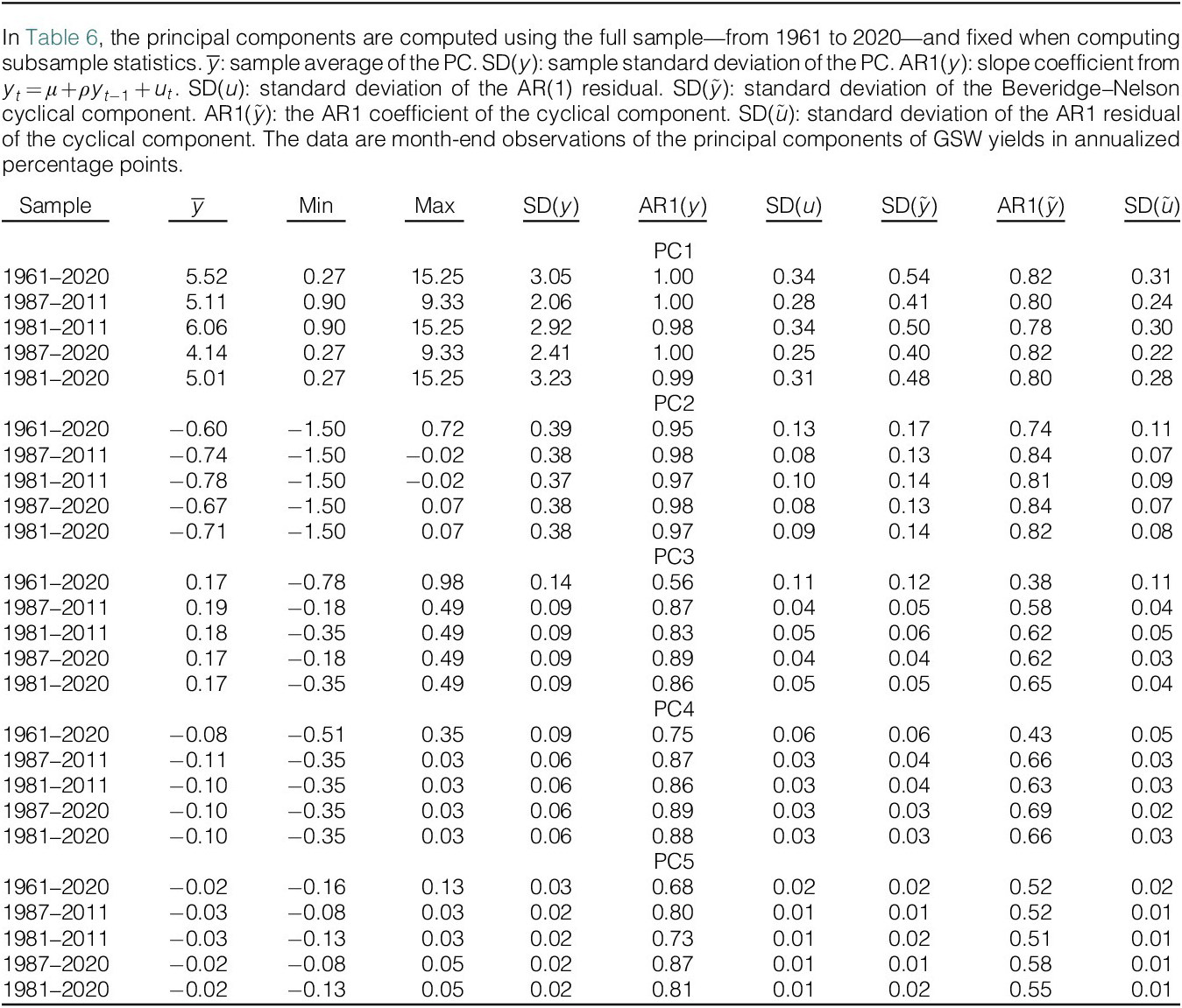
According to equation (12), the value of $ {\mathcal{B}}_n^{rn} $ depends on $ {\boldsymbol{\delta}}_1 $ and the persistence parameter $ \Phi $ of the yield curve PCs. Since $ {\boldsymbol{\delta}}_1 $ is identical across sample periods, $ \Phi $ must be different. Table 6 reports the AR(1) coefficients of the first five yield curve PCs estimated from different samples. To isolate the variation in estimated parameters from the PCs, we fix the latter to be estimated from the full sample, ranging from 1961 to 2020. The average yield (PC1) is highly persistent, with the AR(1) coefficient close to 1 across all sample periods. Similarly, the slope factor (PC2) also shows consistent degrees of persistence throughout the different periods. In contrast, the curvature factor (PC3) has an AR(1) coefficient of 0.56 over the 1961–2020 sample, but this coefficient ranges from 0.83 to 0.89 across other subsamples. Beyond the third PC, higher-order PCs also exhibit significantly different degrees of persistence across subsamples. Therefore, the primary reason for the discrepancies in $ {\mathcal{B}}_n^{rn} $ is that the high-order PCs of the yield curve exhibit different degrees of persistence across sample periods.

TABLE 6Summary Statistics of the Yield Curve Principal Components

TABLE 6 Long description

The table contains summary statistics for five principal components (P C 1, P C 2, P C 3, P C 4, and P C 5). The columns represent: Sample period, y-bar (average), Min, Max, S D (y) (standard deviation), A R 1 (y) (autocorrelation), S D (u) (residual standard deviation), S D (y-tilde) (cyclical standard deviation), A R 1 (y-tilde) (cyclical autocorrelation), and S D (u-tilde) (cyclical residual standard deviation).

* P C 1 (Level): For the full 1961 to 2020 sample, y-bar is 5.52, S D (y) is 3.05, and A R 1 (y) is 1.00. Values for y-bar range from 4.14 to 6.06 across subsamples.

* P C 2 (Slope): For the full sample, y-bar is minus 0.60, S D (y) is 0.39, and A R 1 (y) is 0.95. Subsample y-bar values are consistently negative, ranging from minus 0.78 to minus 0.67.

* P C 3 (Curvature): For the full sample, y-bar is 0.17, S D (y) is 0.14, and A R 1 (y) is 0.56. Subsample y-bar values are stable around 0.17 to 0.19.

* P C 4: For the full sample, y-bar is minus 0.08, S D (y) is 0.09, and A R 1 (y) is 0.75. Subsample y-bar values are approximately minus 0.10.

* P C 5: For the full sample, y-bar is minus 0.02, S D (y) is 0.03, and A R 1 (y) is 0.68. Subsample y-bar values range from minus 0.03 to minus 0.02.

Across all components, the A R 1 (y) values indicate high persistence, particularly in P C 1 and P C 2 where they reach 1.00 and 0.98 respectively.

Why does the shifting endpoint model produce highly consistent risk-neutral rates from different sample periods? Recall that the risk-neutral bond price is $ \ln {P}_t^{(n) rn}={\mathcal{A}}_n+{\mathcal{B}}_n^{rn\top }{X}_t+{\mathcal{C}}_n^{rn}{\tau}_t $ . As shown in Figure 6B, the magnitudes of $ {\mathcal{B}}_n^{rn} $ from the shifting endpoint model are smaller than those from the FE model, and the discrepancies in $ {\mathcal{B}}_n^{rn} $ across sample periods are also reduced. This reduction in variability can be attributed to the fact that $ \Phi $ in the recursion equation (21) is the persistence parameter of the cyclical component $ {\tilde{X}}_t $ , and Table 1 suggests that the cyclical yields are much less persistent than the actual yields. Additionally, Figure 6C shows that $ {\mathcal{C}}_n^{rn} $ remains very similar across samples. Note that $ {\tau}_t $ is the Beveridge–Nelson trend of the first PC of the yield curve, and the two series have similar degrees of variation. The magnitude of $ {\mathcal{C}}^{rn} $ in Figure 6C is larger than that of $ {\mathcal{B}}^{rn}1 $ in Figure 6B, suggesting that the variations of the risk-neutral rates from the ESE model are mainly driven by fluctuations in $ {\tau}_t $ . The consistency of $ {\mathcal{C}}^{rn} $ across estimation samples implies that the estimated risk-neutral rates are robust across sample periods.

B. Estimated States Versus Parameters

Note that the state variables $ {X}_t,{\tau}_t $ are estimated from observed yields, so the parameters producing them may also vary across sample periods. To examine the contributions of the state variables and the yield curve parameters $ {\mathcal{A}}^{rn},{\mathcal{B}}^{rn},{\mathcal{C}}^{rn} $ to the (in)stability of estimated risk-neutral yields, we conduct two exercises.

Fixed parameters. The parameters $ {\mathcal{A}}^{rn},{\mathcal{B}}^{rn},{\mathcal{C}}^{rn} $ are estimated from the 1961–2020 sample. For each subsample, we only re-estimate $ {X}_t $ and $ {\tau}_t $ , and combine them with the fixed $ {\mathcal{A}}^{rn},{\mathcal{B}}^{rn},{\mathcal{C}}^{rn} $ to produce risk-neutral yields.

Fixed states. The state variables $ {X}_t,{\tau}_t $ are estimated from the 1961–2020 sample. For each subsample, the respective $ {X}_t,{\tau}_t $ are extracted from the fixed full sample. Then, we estimate $ {\mathcal{A}}^{rn},{\mathcal{B}}^{rn},{\mathcal{C}}^{rn} $ and combine with the state variables to produce risk-neutral yields.

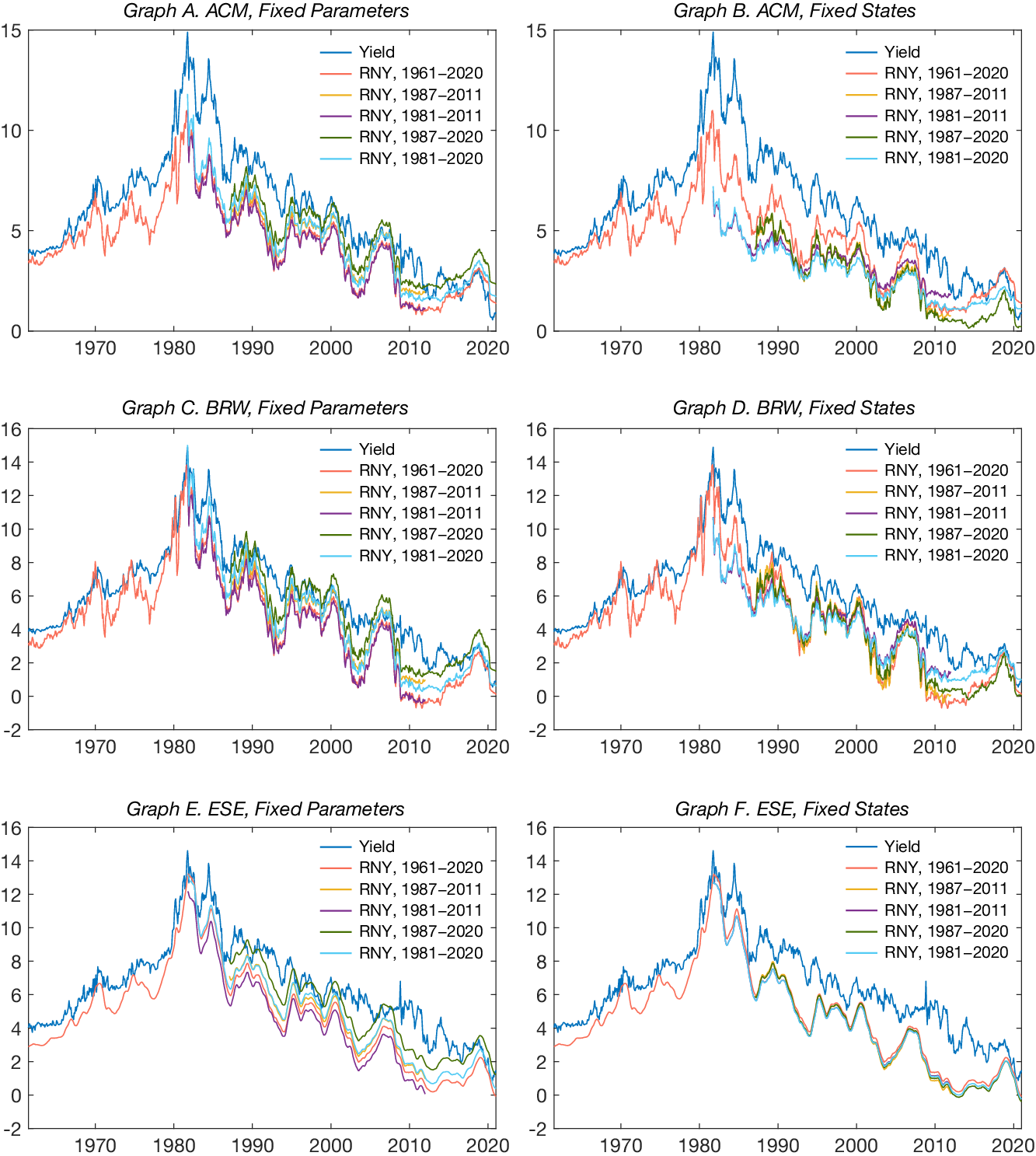
Figure 7 presents the 10-year risk-neutral yields implied by the ACM, BRW, and ESE models. For all models, the fixed-parameter exercise produces unstable risk-neutral yields across subsamples. This reflects the fact that the state variables $ {X}_t $ and $ {\tau}_t $ are estimated and are thus unstable across subsamples. Notice that the shifting-endpoint model does not make the state estimation more stable. On the other hand, the fixed-state exercise forces the state variables to be consistent across subsamples. The variations in the risk-neutral yields across subsamples are solely due to inconsistencies in $ {\mathcal{A}}^{rn},{\mathcal{B}}^{rn},{\mathcal{C}}^{rn} $ . The BRW bias correction makes the yield curve parameters more stable than those implied by the canonical ACM method, but there are still substantial discrepancies in the risk-neutral yields in the 1980s and 2010s. In contrast, the risk-neutral yields implied by the ESE method almost coincide, suggesting more consistent estimates of the yield curve parameters.

FIGURE 7Fixed Parameters or States: 10-Year Risk-Neutral Yield

In Figure 7, ACM: Adrian et al. (Reference Adrian, Crump and Moench2013) fixed-endpoint model. BRW: the ACM fixed-endpoint model adopting the Bauer et al. (Reference Bauer, Rudebusch and Wu2012) correction. ESE: shifting-endpoint model with an estimated trend. Fixed parameters: all subsamples use the parameters $ {\mathcal{A}}^{rn},{\mathcal{B}}^{rn},{\mathcal{C}}^{rn} $ estimated from the 1961–2020 sample. The state variables are estimated separately for each subsample. Fixed states: compute the principal components and $ {\tau}_t $ using the 1961–2020 sample, then take the snapshot according to the subsample periods; the yield curve parameters $ {\mathcal{A}}^{rn},{\mathcal{B}}^{rn},{\mathcal{C}}^{rn} $ are estimated using each snapshot.

FIGURE 7 Long description

A multi-panel figure containing six line graphs labeled Graph A through Graph F. Each graph plots yield percentages on the Y-axis against years from 1961 to 2020 on the X-axis.

* Graph A (A C M, Fixed Parameters) and Graph B (A C M, Fixed States): Y-axis ranges from 0 to 15. Both show a sharp peak around 1981 followed by a long-term decline. Graph B shows more divergence in the R N Y sub-samples after 1990 compared to Graph A.

* Graph C (B R W, Fixed Parameters) and Graph D (B R W, Fixed States): Y-axis ranges from -2 to 16. These models show similar volatility to A C M but with lower troughs, particularly in the 2010 to 2020 period where some R N Y lines dip toward zero.

* Graph E (E S E, Fixed Parameters) and Graph F (E S E, Fixed States): Y-axis ranges from -2 to 16. Graph E shows a distinct vertical spread between the different R N Y sub-samples (1961-2020, 1987-2011, 1981-2011, 1987-2020, and 1981-2020). Graph F shows these lines tightly clustered, nearly overlapping the main Yield line after 1990.

Common Legend: A dark blue line represents Yield. Other colored lines represent R N Y (Risk-Neutral Yield) for various time intervals: 1961-2020 (red), 1987-2011 (yellow), 1981-2011 (purple), 1987-2020 (green), and 1981-2020 (light blue).

C. Monetary Policy Transmission

Finally, we investigate why the estimated effects of monetary policy shocks on FE risk-neutral yields are sensitive to the sample periods for estimating the risk-neutral yields and why the results for the OSE risk-neutral yields are more stable.

The FE model implies that the risk-neutral yields are

(25) $$ {y}_t^{(n) rn}={A}_n^{rn}+{B}_n^{rn\top }{X}_t, $$

and the OSE model implies

(26) $$ {y}_t^{(n) rn}={A}_n^{rn}+{B}_n^{rn\top }{X}_t+{C}_n^{rn}{\tau}_t, $$

with $ {A}_n^{rn}=-\frac{1}{n}{\mathcal{A}}_n^{rn} $ , $ {B}_n^{rn}=-\frac{1}{n}{\mathcal{B}}_n^{rn} $ , and $ {C}_n^{rn}=-\frac{1}{n}{\mathcal{C}}_n^{rn} $ . We investigate how the responses of $ {X}_t,{\tau}_t $ and $ {B}_{n,i}^{rn}{X}_{i,t},{C}_n^{rn}{\tau}_t $ depend on the sample periods. Since the “fixed states” exercise mechanically generates identical responses of the state variables across sample periods, we jointly estimate the state variables and model parameters on each subsample, and then regress the model-implied risk-neutral yields on the high-frequency monetary policy shocks.

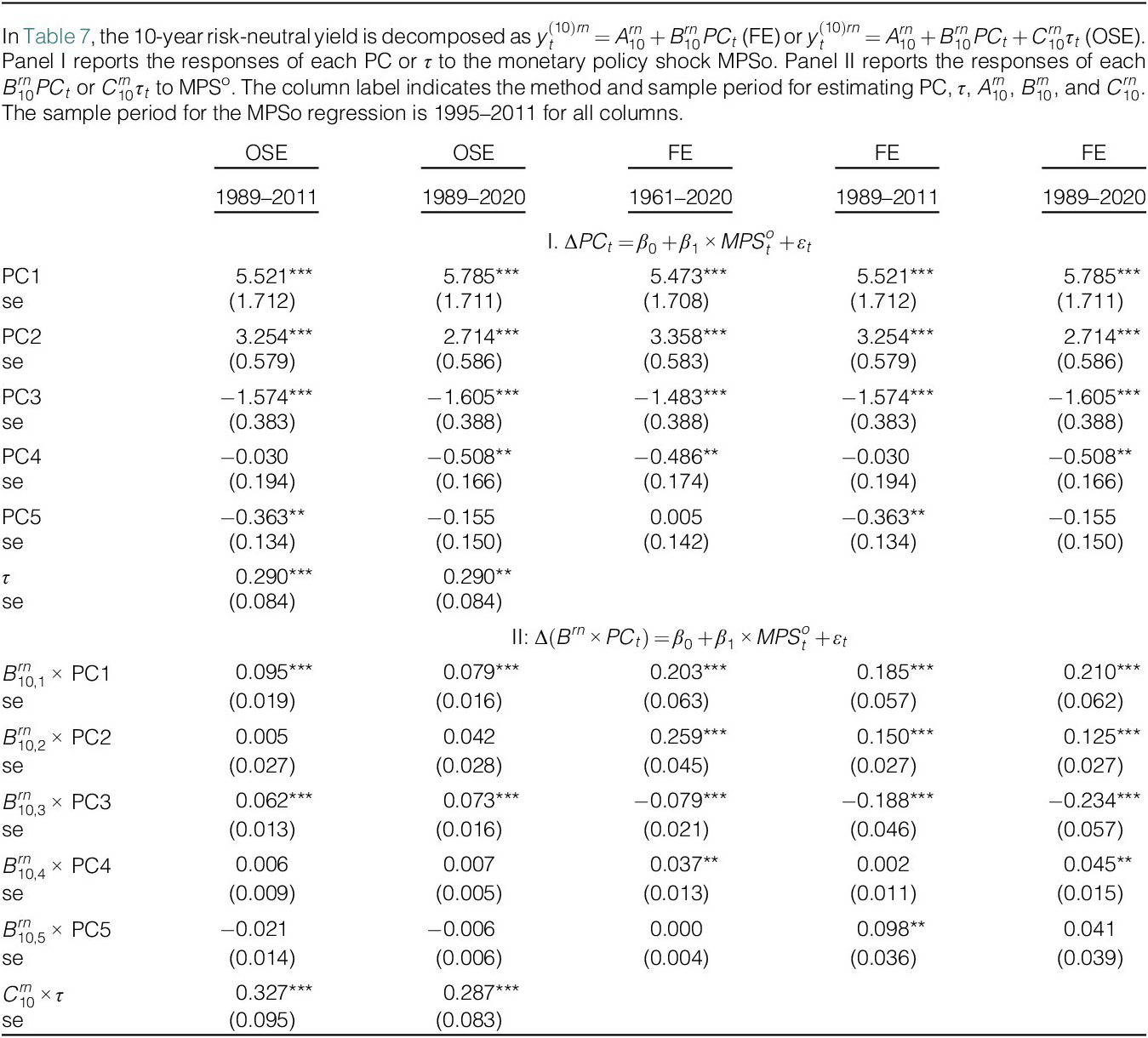
Table 7 reports the response of the estimated 10-year risk-neutral yield to MPSo, the first PC of Eurodollar shocks. Among the state variables, the level (PC1) and slope (PC2) factors are the most responsive to the monetary policy shock, and the response of the slope factor is the most sensitive to sample periods in absolute terms. In the FE model, the variation in $ {B}_n^{rn} $ amplifies the sensitivity of the estimated risk-neutral yields’ responses to sample periods. According to the FE model, the response of $ {B}_{10,2}^{rn}\times PC{2}_t $ varies by more than 100% across sample periods, and the higher-order PCs times the respective $ {B}_n^{rn} $ vary by even more percentages. The responses of the $ {B}_n^{rn}{PC}_t $ components in the OSE model are also sensitive to the sample periods, but are orders of magnitude smaller than in the FE model. Instead, the response of $ {C}_n^{rn}{\tau}_t $ is large and stable, significantly reducing the variation in the risk-neutral yield across sample periods.

TABLE 7Decomposing the 10-Year RNY Response to MPSo

TABLE 7 Long description

The table is organized into two main panels across five columns. The columns are categorized by method and sample period: O S E 1989–2011, O S E 1989–2020, F E 1961–2020, F E 1989–2011, and F E 1989–2020.

Panel I analyzes the regression Delta P C sub t = beta sub 0 + beta sub 1 times M P S super o sub t + epsilon sub t.

* P C 1 values range from 5.473 to 5.785, all significant at the 0.01 level.

* P C 2 values range from 2.714 to 3.358, all significant at the 0.01 level.

* P C 3 values are negative, ranging from -1.483 to -1.605, all significant at the 0.01 level.

* P C 4 and P C 5 show varying significance, with P C 4 being significant in the 1989–2020 and 1961–2020 samples.

* Tau is reported only for O S E columns at 0.290.

Panel II analyzes the regression Delta (B super r n times P C sub t) = beta sub 0 + beta sub 1 times M P S super o sub t + epsilon sub t.

* B sub 10,1 super r n times P C 1 shows positive coefficients across all columns, ranging from 0.079 to 0.210.

* B sub 10,2 super r n times P C 2 is significant only in the F E columns (0.125 to 0.259).

* B sub 10,3 super r n times P C 3 shows positive coefficients for O S E (0.062 to 0.073) but negative coefficients for F E (-0.079 to -0.234).

* C sub 10 super r n times tau is reported for O S E at 0.327 and 0.287, both significant at the 0.01 level.

Standard errors (s e) are provided in parentheses below each coefficient.

This decomposition clarifies why the shifting-endpoint model’s results merit greater confidence: its primary driver of responses to policy shocks—the $ {\tau}_t $ term—is stable across sample periods, ensuring robustness of the estimated policy channel. By contrast, FE’s reliance on unstable PCs amplifies sample-period sensitivity, making its estimates far less reliable when long historical data are unavailable.

A. Time Series of Risk-Neutral Rates

We focus on the domestic currency nominal sovereign yields of the G10 countries: Australia (AUD), Canada (CAD), Switzerland (CHF), Denmark (DKK), the Eurozone/Germany (EUR), the United Kingdom (GBP), Japan (JPY), Norway (NOK), New Zealand (NZD), and Sweden (SEK). The sovereign yield data are updated from Du et al. (Reference Du, Im and Schreger2018). For most countries, the sample starts in the early 1990s. For Norway, the sample starts in 1998. For Canada and the United Kingdom, we obtain the yield curve data from the respective central bank’s website, which start earlier than the Bloomberg data. The Canadian yield curve starts in January 1986, and the U.K. yield curve starts in January 1979.

We consider the following three specifications of sample periods:

• • Earliest observation: 2020.

• • Earliest observation: 2011. The sample stops at the end of the Adrian et al. (Reference Adrian, Crump and Moench2013) sample.

• • 2001–2020: The sample has roughly the same length as the previous one but covers the later part of the full sample.

We begin by estimating the FE model for each G10 country individually. Figure 8 presents the observed yields alongside their risk-neutral components, estimated from the FE model using different samples. The risk-neutral rates for some countries show significantly larger discrepancies than those observed for the United States during the post-1990 period. For instance, the 10-year risk-neutral rates of Australia, Switzerland, and Denmark appear essentially flat when estimated using the start-2011 sample. However, when estimated using the start-to-2020 sample, these rates exhibit much stronger downward trends and cyclical fluctuations. The discrepancies in the 5-5 risk-neutral forward rates are even more pronounced. For example, in September 2011, the 5-5 risk-neutral forward rates estimated from the start-to-2011 sample and the 2000–2020 sample differ by 1.42 percentage points, which represents 266% of the latter’s value. In several countries—including Australia, Switzerland, Denmark, the Eurozone, Norway, New Zealand, and Sweden—the maximum vertical difference in the 5-5 risk-neutral forward rates, when estimated using these two samples, exceeds 100% of the value derived from the 2000–2020 sample. Notably, Sweden experiences a staggering 2676% difference. In absolute terms, New Zealand has the maximum difference of 3.86 percentage points, which was recorded in December 2011.

FIGURE 8FE Risk-Neutral Yields Estimated on Different Samples

In Figure 8, the risk-neutral yields are estimated country-by-country from the FE model. The term structure model is the canonical Adrian et. al (Reference Adrian, Crump and Moench2013) model. The “Yield” series are the observed yields.

FIGURE 8 Long description

The figure consists of 22 individual line graphs organized into two columns: Graph A. 10-Year Yield and Graph B. 5-5 Forward Rate. Each column contains 11 panels corresponding to currencies: A U D, C A D, C H F, D K K, E U R, G B P, J P Y, N O K, N Z D, S E K, and U S D.

* Axes and Legend: The X-axis represents years, typically ranging from the early 1990s to 2020, though G B P starts in 1980. The Y-axis represents percentage yields. A shared legend at the bottom of each column identifies four lines: a dark blue line for Yield, a red line for R N Y start-2020, a yellow line for R N Y start-2011, and a purple line for R N Y 2000-2020.

* Data Trends in Graph A: Across all currencies, the dark blue Yield line shows a consistent long-term downward trend, starting between 5 and 15 percent and ending near or below 0 percent by 2020. The R N Y (Risk-Neutral Yield) estimates generally track below the actual yield. The yellow line (start-2011) often terminates earlier than the others. The red and purple lines show high correlation, frequently overlapping as they decline toward zero.

* Data Trends in Graph B: The 5-5 Forward Rates mirror the downward trajectory seen in Graph A but often exhibit higher volatility in the early years. In several panels like A U D and C H F, the yellow R N Y line appears as a flat horizontal segment during the mid-2000s before resuming a downward slope. By 2020, almost all metrics across all currencies converge at their lowest historical points, with many R N Y estimates dipping into negative territory for C H F, D K K, and E U R.

Next, we estimate the ESE model on a country-by-country basis. Figure 9 displays the risk-neutral 10-year yield and the 5-5 forward rates estimated from different sample periods. While the ESE risk-neutral rates do not coincide perfectly across samples, they demonstrate significantly greater robustness to the specification of sample periods than the FE risk-neutral rates. Additionally, the ESE risk-neutral rates reveal stronger downward trends than their FE counterparts. In this international context, our findings align with those of Bauer and Rudebusch (Reference Bauer and Rudebusch2020), indicating that the shifting endpoint model attributes a larger fraction of the observed decline in long-term yields to the expectations component than the FE model does.

FIGURE 9ESE Risk-Neutral Yields Estimated on Different Samples

In Figure 9, the risk-neutral yields are estimated country-by-country from the ESE model. The term structure model is the Bauer and Rudebusch (Reference Bauer and Rudebusch2020) model. The “Yield” series are the observed yields.

FIGURE 9 Long description

The figure contains twenty-two subplots organized into two main columns: Graph A. 10-Year Yield and Graph B. 5-5 Forward Rate. Each column contains eleven subplots for currencies: A U D, C A D, C H F, D K K, E U R, G B P, J P Y, N O K, N Z D, S E K, and U S D.

Each subplot features an x-axis representing years (ranging from approximately 1980 to 2020 depending on the currency) and a y-axis representing percentage yields. Four lines are plotted in each graph:

* A dark teal line representing the actual Yield.

* An orange line representing R N Y, start-2020.

* A yellow line representing R N Y, start-2011.

* A purple line representing R N Y, 2000-2020.

Across all currencies and both graph types, there is a consistent downward trend from high yields (often between 10 and 15 percent in the 1980s and 1990s) toward near-zero or slightly negative yields by 2020. The teal Yield line typically remains the highest, while the various R N Y (Risk-Neutral Yield) estimates track below it, showing significant volatility and convergence in the later years of the sample. The G B P and C A D plots show the longest historical data starting from 1980, while others like N O K and E U R begin around 1995 to 2000.

B. U.S. Monetary Policy Spillover

The global financial cycle literature documents that U.S. monetary policy shocks significantly affect international long-term yields. How much of the spillover effect is attributable to interest rate expectations? We estimate the regression

(27) $$ \Delta {y}_{i,t}={\beta}_0+{\beta}_1{MPS}_t^o+{\varepsilon}_t $$

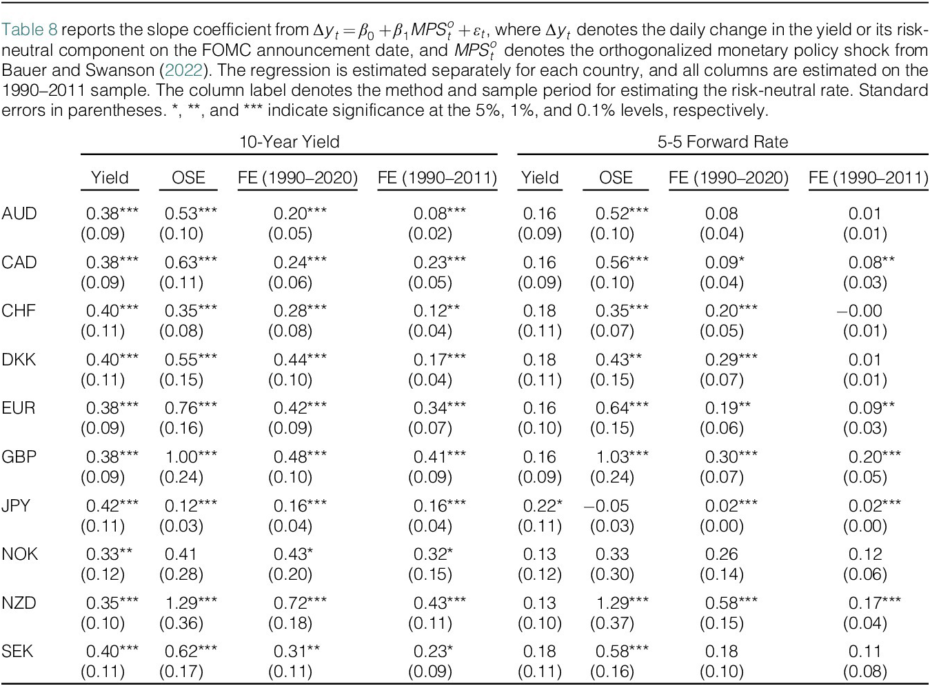
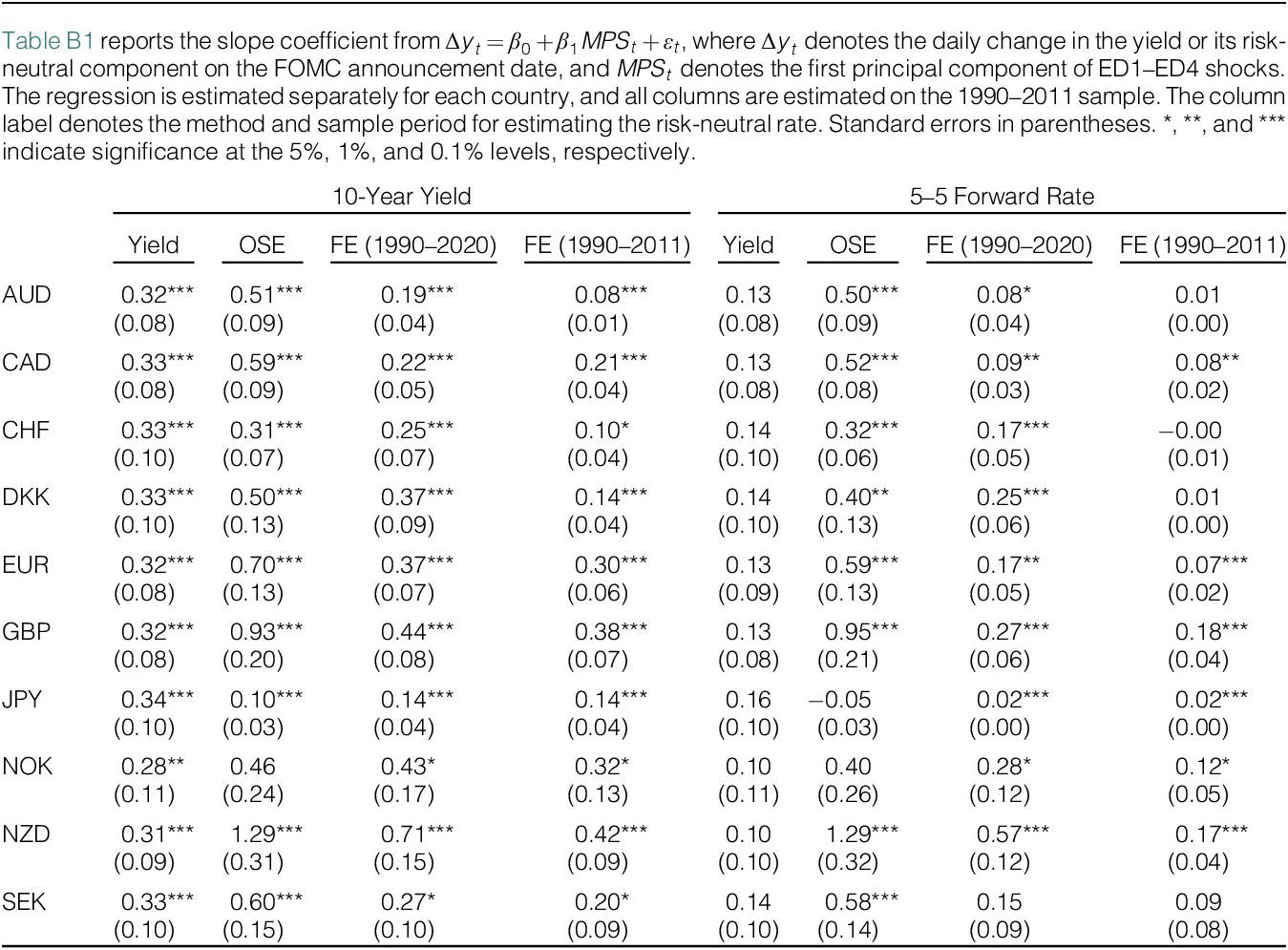
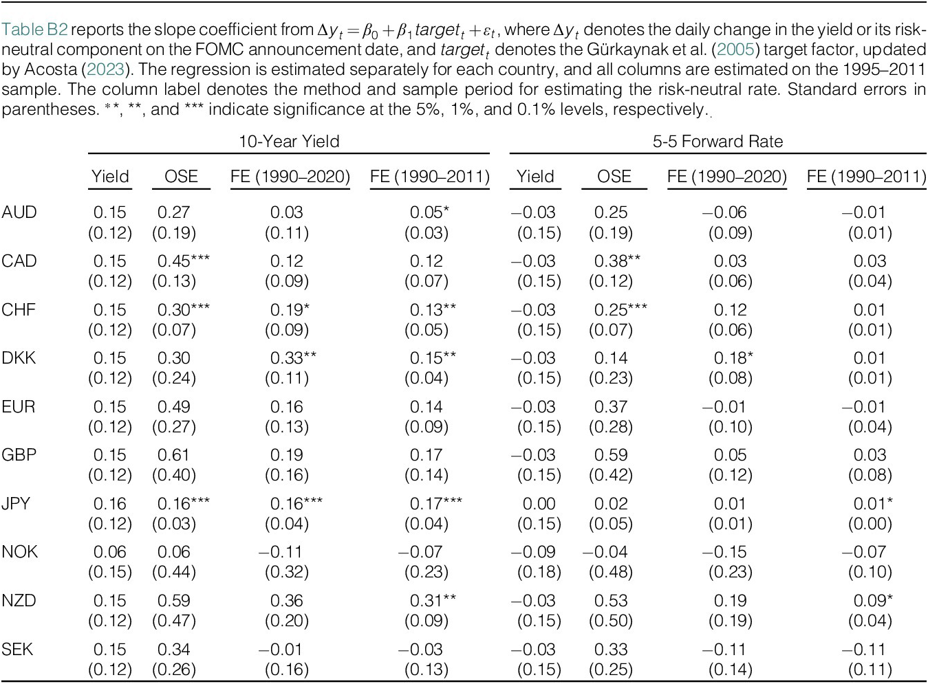
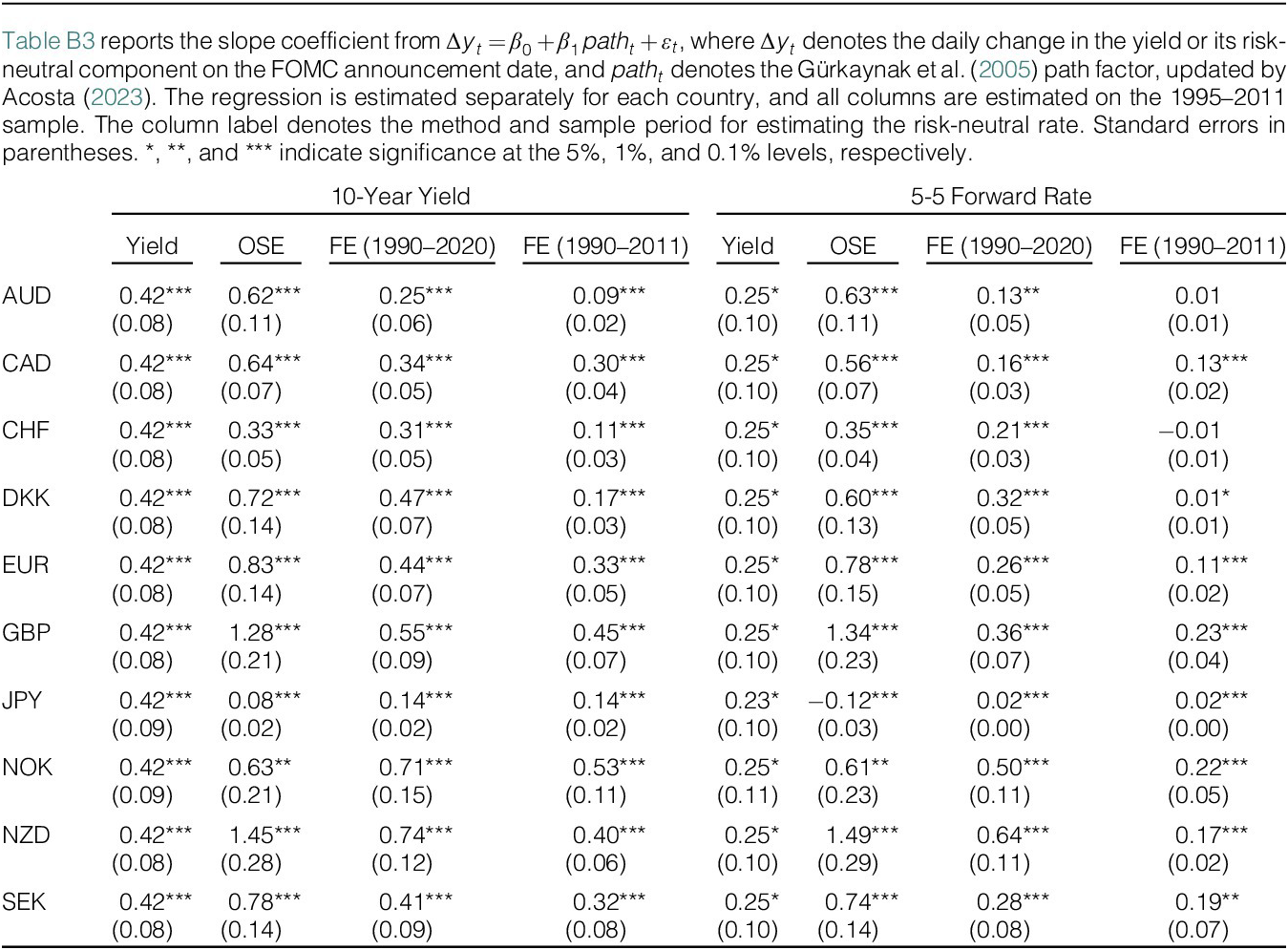
for each country, where $ \Delta {y}_{i,t} $ is the daily change in a long-term yield or its risk-neutral component of country $ i $ on the FOMC announcement date, and $ {MPS}_t^o $ is the orthogonalized monetary policy shock from Bauer and Swanson (Reference Bauer, Swanson, Eichenbaum, Hurst and Ramey2022). The sample for estimating equation (27) is 1990–2011, and we consider two alternative sample periods for estimating the FE risk-neutral rates: 1990–2020 and 1990–2011. In Appendix B, we present the spillover effects of other high-frequency measures of U.S. monetary policy shocks.

Table 8 reports the estimation results for the slope coefficient. We focus on the 10-year yield and the 5-5 forward rate. For each yield, the first column uses the daily change in the yield as the dependent variable, and the other columns use the daily change in the risk-neutral rate as the dependent variable. U.S. monetary policy shocks significantly affect G10 countries’ 10-year yields, but the effects on the 5-5 forward rates are smaller and insignificant. The estimated responses of international FE risk-neutral rates to U.S. monetary policy shocks are not robust to the choice of sample periods, although the sample periods for estimating risk-neutral rates only differ by 9 years. For example, the estimated values of $ {\hat{\beta}}_1 $ for Switzerland and Denmark’s 10-year FE risk-neutral rates differ by more than two times across the sample periods. The contrasts for the 5-5 risk-neutral forward rates are stronger, but the estimates of $ {\hat{\beta}}_1 $ are noisier.

TABLE 8International Transmission of U.S. Monetary Policy Shock

TABLE 8 Long description

The table presents regression slope coefficients for the impact of U. S. monetary policy shocks on international yields.

Header Structure:

Columns are divided into two main categories: 10-Year Yield and 5-5 Forward Rate. Each category has four sub-columns: Yield, O S E, F E 1990–2020, and F E 1990–2011.

Data Rows (Coefficient followed by Standard Error in parentheses):

• A U D: 10-Year Yields range from 0.08 to 0.53; 5-5 Forward Rates range from 0.01 to 0.52.

• C A D: 10-Year Yields range from 0.23 to 0.63; 5-5 Forward Rates range from 0.08 to 0.56.

• C H F: 10-Year Yields range from 0.12 to 0.40; 5-5 Forward Rates range from -0.00 to 0.35.

• D K K: 10-Year Yields range from 0.17 to 0.55; 5-5 Forward Rates range from 0.01 to 0.43.

• E U R: 10-Year Yields range from 0.34 to 0.76; 5-5 Forward Rates range from 0.09 to 0.64.

• G B P: 10-Year Yields range from 0.38 to 1.00; 5-5 Forward Rates range from 0.16 to 1.03.

• J P Y: 10-Year Yields range from 0.12 to 0.42; 5-5 Forward Rates range from -0.05 to 0.22.

• N O K: 10-Year Yields range from 0.32 to 0.43; 5-5 Forward Rates range from 0.12 to 0.33.

• N Z D: 10-Year Yields range from 0.35 to 1.29; 5-5 Forward Rates range from 0.13 to 1.29.

• S E K: 10-Year Yields range from 0.23 to 0.62; 5-5 Forward Rates range from 0.11 to 0.58.

Statistical significance is indicated by asterisks: * for 5 percent, ** for 1 percent, and *** for 0.1 percent levels.