


1. Introduction
Spontaneous imbibition is a phenomenon whereby a wetting fluid driven by capillary force enters capillaries or porous media to displace the in situ fluid. Because of its widespread presence in natural and industrial processes, such as enhanced oil recovery (Tavassoli, Zimmerman & Blunt Reference Tavassoli, Zimmerman and Blunt2005; Xu et al. Reference Xu, Bai, Wu, Hou, Meng, Sun, Li, Lu and Kang2019), underground gas storage (Guo et al. Reference Guo, Bandilla, Nordbotten, Celia, Keilegavlen and Doster2016), inkjet printing (Wijshoff Reference Wijshoff2018) and water uptake in plant tissues (Finch-Savage, Rowse & Dent Reference Finch-Savage, Rowse and Dent2005), spontaneous imbibition has received extensive attention for more than a century (Bell & Cameron Reference Bell and Cameron1906; Zhao et al. Reference Zhao, Qin, Fischer, Kang, Derome and Carmeliet2021). For spontaneous imbibition in a circular capillary with high viscosity ratio of wetting to non-wetting fluids, the well-known Lucas–Washburn equation shows that the imbibition length is proportional to the square root of time, with the proportionality factor given by  $(\sigma R \cos \theta /2\mu _R)^{1/2}$, where
 $\sigma$,
 $\theta$,
 $\mu _R$ and
 $R$ are the surface tension coefficient, the contact angle measured from the wetting fluid side, the dynamic viscosity of the wetting fluid and the radius of the capillary, respectively (Lucas Reference Lucas1918; Bell & Cameron Reference Bell and Cameron1906; Washburn Reference Washburn1921). However, when it comes to porous media, the imbibition dynamics becomes complicated as the invasion process is related to many factors, such as the geometric characteristics and connectivity of porous media (Sadjadi & Rieger Reference Sadjadi and Rieger2013; Chang & Kim Reference Chang and Kim2020), the wettability of the solid surface (Andersen & Ahmed Reference Andersen and Ahmed2021; Mason & Morrow Reference Mason and Morrow2013) and the physicochemical properties of the fluids (Høgnesen, Standnes & Austad Reference Høgnesen, Standnes and Austad2004). Due to the inherent complexity, spontaneous imbibition in porous media remains not fully understood, especially with regard to the exact scaling law for the imbibed amount of the wetting fluid and to the associated displacement patterns.
Extensive works have been done to comprehend two-phase displacement in porous media, and three typical displacement patterns, namely capillary fingering, viscous fingering and compact displacement (also known as stable displacement), are identified in drainage or forced imbibition, which strongly depend on the capillary number and viscosity ratio (Lenormand, Touboul & Zarcone Reference Lenormand, Touboul and Zarcone1988; Riaz et al. Reference Riaz, Tang, Tchelepi and Kovscek2007; Zhang et al. Reference Zhang, Oostrom, Wietsma, Grate and Warner2011; Sharma, Inwood & Kovscek Reference Sharma, Inwood and Kovscek2012; Hu et al. Reference Hu, Lan, Wei and Chen2019, Reference Hu, Patmonoaji, Zhang and Suekane2020; Xiao et al. Reference Xiao, Zhu, Zhang, Yao and Sun2021). Unlike drainage and forced imbibition, spontaneous imbibition does not impose a fixed injection velocity at the inlet boundary, so the capillary number cannot be defined. In this context, existing studies of spontaneous imbibition were mainly concerned about the viscosity ratio. For example, Sun, Kharaghani & Tsotsas (Reference Sun, Kharaghani and Tsotsas2016) conducted a spontaneous imbibition experiment with an air-filled micromodel invaded by mixtures of ethanol and water with various proportions, and showed that compact displacement with relatively flat advancement of wetting front occurs when the viscosity ratio of wetting to non-wetting fluids is much greater than  $1$. By changing the viscosity ratio, Liu et al. (Reference Liu, Sun, Wu, Wei and Hou2021) numerically observed unstable fingering and compact displacement for spontaneous imbibition in a micromodel with regular pore geometries. On the other hand, as emphasised by Golmohammadi et al. (Reference Golmohammadi, Ding, Kuechler, Reuter, Schlueter, Amro and Geistlinger2021), the gravitational force could lead to the instability of the advancing front in a vertical imbibition process, thus altering the displacement pattern. This factor, however, is always ignored in previous studies of spontaneous imbibition and is worthy of further exploration.
In compact displacement, the wetting front progresses uniformly in one direction, indicating one-dimensional (1-D) flow characteristics (Kang et al. Reference Kang, Perfect, Cheng, Bilheux, Gragg, Wright, Lamanna, Horita and Warren2013; Sun et al. Reference Sun, Kharaghani and Tsotsas2016). Due to the 1-D similarity of compact displacement to capillary-driven flow in a single circular capillary, researchers have extended the Lucas–Washburn equation to the quantification of compact displacement in porous media by considering the geometrical complexity of the pore structure (Cai et al. Reference Cai, Jin, Kou, Zou, Xiao and Meng2021). Typically, the geometrical complexity can be considered by using the equivalent radius derived from the fractal geometry theory (Cai et al. Reference Cai, Yu, Zou and Luo2010; Li & Zhao Reference Li and Zhao2012; Shi, Yassin & Dehghanpour Reference Shi, Yassin and Dehghanpour2018; Wang & Zhao Reference Wang and Zhao2021), or by using an effective hydraulic radius computed from the macroscopic properties of porous media, including the permeability, porosity, pore shape and so on (Benavente et al. Reference Benavente, Lock, Del Cura and Ordóñez2002; Fries & Dreyer Reference Fries and Dreyer2008; Babchin et al. Reference Babchin, Bentsen, Faybishenko and Geilikman2016). However, the former suffers from ignoring the connectivity of porous media, since a porous medium is ideally simplified as a bundle of capillaries without interaction in the fractal geometry theory. The latter preserves the connectivity of porous media, but cannot fully consider the geometric characteristics and wettability of the pore structure. Specifically, the Hagen–Poiseuille assumption for evaluating viscous pressure drop makes the extended Lucas–Washburn equation inaccurate when applied to thin porous media, e.g. a micromodel, because the viscous force in a rectangular capillary is entirely different from that in a circular capillary (Ouali et al. Reference Ouali, McHale, Javed, Trabi, Shirtcliffe and Newton2013). In addition, recent studies showed that using a geometrical apparent contact angle to represent the wettability of complex porous media is inaccurate (Blunt et al. Reference Blunt, Lin, Akai and Bijeljic2019; Hou et al. Reference Hou, Zhang, Sun, Wang, Wang, Zhang and Li2020; Sun et al. Reference Sun, McClure, Mostaghimi, Herring, Berg and Armstrong2020). Thus, methods based on energy analysis have been developed to improve the accuracy of measuring the wettability of porous media in spontaneous imbibition (Blunt et al. Reference Blunt, Lin, Akai and Bijeljic2019, Reference Blunt, Alhosani, Lin, Scanziani and Bijeljic2021; Alinejad & Dehghanpour Reference Alinejad and Dehghanpour2021), but the impact of viscous dissipation which is hard to evaluate is neglected in such energy analysis (Akai et al. Reference Akai, Lin, Bijeljic and Blunt2020). To deepen the understanding of spontaneous imbibition in complex porous media where flow channels are of non-circular cross-sections, it is critical to fully consider the geometric and wetting characteristics at the pore scale and to develop a new theoretical model for the accurate prediction of the compact displacement process.
In the past 30 years, porous media micromodels have been increasingly applied to fundamental research activities (Karadimitriou & Hassanizadeh Reference Karadimitriou and Hassanizadeh2012; Gogoi & Gogoi Reference Gogoi and Gogoi2019; Zhu et al. Reference Zhu, Wang, Yan, Liu, Zhu and Chen2022) and many industrial fields, such as the food and wood industries (Anbari et al. Reference Anbari, Chien, Datta, Deng, Weitz and Fan2018), for the understanding of multiphase flow behaviour inside microstructures. The use of micromodels for pore-scale study has many unique advantages, which mainly include the following. (1) Direct visualisation of the transient fluid distribution without special microtomography equipment. This means that one can easily observe displacement scenarios at the pore scale, and measure the multiphase flow properties, such as the fluid saturation, interfacial area and so on. Many typical geophysical flow phenomena, e.g. Haines jumps, were found to cascade through 10–20 geometrically defined pores (Berg et al. Reference Berg2013; Armstrong et al. Reference Armstrong, Evseev, Koroteev and Berg2015; Li et al. Reference Li, Kazemifar, Blois and Christensen2017), and it is very expensive and challenging to implement real-time three-dimensional (3-D) microtomography over such a large domain. (2) Independent manipulation of the properties of porous media, such as the porosity, pore-throat size and shape, connectivity and wetting properties, which are not limited by the inherent properties of natural porous media. This makes it possible to separately investigate the influence of each factor on the displacement process. (3) Convenient construction of the digital pore network geometry. Benefiting from this, one can easily conduct direct numerical simulation of the digital micromodel geometry, and the images obtained from micromodel visualisation experiments could serve as benchmark solutions for the assessment of numerical models or methods. Because of these significant advantages, micromodels have been extensively used in numerical and experimental studies (Alizadeh & Fatemi Reference Alizadeh and Fatemi2021; Chen et al. Reference Chen, Huang, Mo, Xue, Liu and Chen2021; Liu et al. Reference Liu, Sun, Wu, Wei and Hou2021; Wang, Mehmani & Xu Reference Wang, Mehmani and Xu2021; Xie et al. Reference Xie, Lei, Balhoff, Wang and Chen2021; Mohammadi, Nikbin-Fashkacheh & Mahani Reference Mohammadi, Nikbin-Fashkacheh and Mahani2022; Otumudia et al. Reference Otumudia, Hamidi, Jadhawar and Wu2022; Zhang et al. Reference Zhang, Su, Li, Da, Hao, Wang, Liu, Gao, Zhao and Wang2022). Despite widespread use, the spontaneous imbibition process in micromodels is still not well understood, especially in the presence of gravity.
Pore-scale simulation has emerged as a powerful tool to complement theoretical and experimental studies. It can not only provide simultaneous information on fluid distribution, flow velocity and pressure, but also reproduce pore-level flow phenomena, such as preferential flow paths, trapping events and the capillary valve effect, which are crucial for macroscopic displacement behaviour and efficiency. A number of numerical approaches have been developed for pore-scale simulation of two-phase flows in porous media, including the pore-network model (Gruener et al. Reference Gruener, Sadjadi, Hermes, Kityk, Knorr, Egelhaaf, Rieger and Huber2012; Joekar-Niasar & Hassanizadeh Reference Joekar-Niasar and Hassanizadeh2012; Sun et al. Reference Sun, Kharaghani and Tsotsas2016; Qin & van Brummelen Reference Qin and van Brummelen2019; Qin et al. Reference Qin, Wang, Hefny, Zhao, Chen and Guo2022), the lattice Boltzmann method (LBM) (Gunstensen et al. Reference Gunstensen, Rothman, Zaleski and Zanetti1991; Sukop et al. Reference Sukop, Huang, Lin, Deo, Oh and Miller2008; Porter, Schaap & Wildenschild Reference Porter, Schaap and Wildenschild2009; Boek & Venturoli Reference Boek and Venturoli2010; Jiang & Tsuji Reference Jiang and Tsuji2015; Zheng, Ju & Wang Reference Zheng, Ju and Wang2018) and traditional computational fluid dynamics methods like volume-of-fluid (Raeini, Blunt & Bijeljic Reference Raeini, Blunt and Bijeljic2012; Yin et al. Reference Yin, Zarikos, Karadimitriou, Raoof and Hassanizadeh2019), level set (Prodanović & Bryant Reference Prodanović and Bryant2006; Jettestuen, Helland & Prodanović Reference Jettestuen, Helland and Prodanović2013) and phase-field (Badalassi, Ceniceros & Banerjee Reference Badalassi, Ceniceros and Banerjee2003; Akhlaghi Amiri & Hamouda Reference Akhlaghi Amiri and Hamouda2013) methods. Among these approaches, the LBM is the most popular one owing to its simplicity in treating complex pore geometries coupled with interfacial dynamics (Chen & Doolen Reference Chen and Doolen1998; Liu et al. Reference Liu, Kang, Leonardi, Schmieschek, Narvaez, Jones, Williams, Valocchi and Harting2016). It also allows for direct simulation in realistic pore geometries obtained from image data, making it possible to directly compare with experimental results and serve as an alternative to pore-scale experiments. To minimise the computational cost, two-dimensional (2-D) LBM simulations have been widely used for the investigation of two-phase flows through porous media and have had great success (Zhao et al. Reference Zhao2019). However, 3-D effects such as the depth-oriented interface curvature and the viscous resistance from top and bottom walls are essential for the successful simulation of spontaneous imbibition in porous media micromodels (Liu et al. Reference Liu, Sun, Wu, Wei and Hou2021). Therefore, the recently developed quasi-three-dimensional (quasi-3D) colour-gradient LBM (Liu et al. Reference Liu, Sun, Wu, Wei and Hou2021), which incurs 2-D computational cost only but accounts for the essential 3-D effects, will be adopted as our simulation tool. Because the depth-averaged assumption is involved in the derivation of the quasi-3D method, it is only applicable to two-phase flows in a micromodel or channel with low aspect ratio. So an open question is how low is the eligible aspect ratio for the application of the quasi-3D method, which will be clarified with the help of the developed theoretical model.
In this paper, a theoretical model for spontaneous imbibition in porous media micromodels is presented, which is developed from the model of a single rectangular capillary while incorporating porosity and permeability for the viscous pressure drop and an equivalent contact angle for the effective capillary force. Focusing on spontaneous imbibition in a single rectangular capillary, we first establish the application condition of the quasi-3D colour-gradient LBM by comparing the simulated results with the theoretical solutions for various aspect ratios. We then simulate spontaneous imbibition in micromodels with various geometries and flow conditions. Different displacement patterns are identified for varying viscosity ratios and gravitational accelerations. For the compact displacement process, we demonstrate that the developed theoretical model provides an accurate prediction of the imbibition length as a function of the time. Finally, the developed theoretical model and LBM simulation are further verified by reproducing the results of micromodel experiments.
2. Theoretical model for spontaneous imbibition in rectangular capillary and micromodel
Given that the micromodel is composed of interconnected rectangular channels, we first consider the imbibition dynamics in a single rectangular capillary. As sketched in figure 1, the wetting (red) fluid is spontaneously imbibed into the rectangular capillary to displace the non-wetting (blue) fluid. The capillary has a length of  $L$, a width of
 $w_s$ and a depth of
 $h$. At time
 $t$, the imbibition length of the wetting fluid is
 $l$. The capillary pressure across a quasi-static interface can be calculated using the interface shape. Although some mathematical attempts have been made (Ajaev & Homsy Reference Ajaev and Homsy2001a,Reference Ajaev and Homsyb), it is still difficult to formulate the accurate interface shape and thus the capillary pressure for a rectangular channel with arbitrary aspect ratio (Ichikawa, Hosokawa & Maeda Reference Ichikawa, Hosokawa and Maeda2004). Therefore, we simplify the pressure difference calculation in a rectangular capillary using two orthogonal principal radii of curvature, with one in the horizontal direction and the other in the depth direction (Anoop & Sen Reference Anoop and Sen2015). According to the Young–Laplace equation, the pressure difference across the interface can be written as
 \begin{equation} \Delta P_{Lap} = \frac{2\sigma \cos \theta} {h} + \frac{2\sigma \cos \theta} {w_s}, \end{equation}
where  $\theta$ is the contact angle measured from the wetting fluid side and
 $\sigma$ is the surface tension coefficient. Then, the capillary driving force
 $F_{Lap}$ can be calculated as
 \begin{equation} F_{Lap} = \Delta P_{Lap} w_s h=2\sigma \cos \theta \left( w_s + h\right) . \end{equation}
According to Ouali et al. (Reference Ouali, McHale, Javed, Trabi, Shirtcliffe and Newton2013), the viscous resistance of the fluid system can be evaluated by
 \begin{equation} F_{vis} ={-} \left[ \frac{12\bar{u} \mu_R l}{\varepsilon \xi\left( \varepsilon\right) } +\frac{12\bar{u} \mu_B \left( L-l\right) }{\varepsilon \xi\left( \varepsilon\right) } \right] \end{equation}
with
 \begin{equation} \xi\left( \varepsilon\right) = \frac{1}{1+0.362374\varepsilon+1.020980\varepsilon^2}, \end{equation}
where  $\bar {u}$ is the mean velocity of the interface,
 $\varepsilon = h/w_s$ is the aspect ratio of the capillary and
 $\mu _R$ and
 $\mu _B$ are the dynamic viscosities of wetting and non-wetting fluids, respectively. For a vertically placed capillary with the inlet connected to the bottom supply, the effect of gravity has to be considered. Here, gravity is only applied to the more viscous fluid (Xiao, Cai & Xu Reference Xiao, Cai and Xu2018), as its influence on the less viscous fluid is so small that it can be ignored safely in commonly seen gas–liquid imbibition systems. In this manner, the gravity
 $G$ can be expressed as
 \begin{equation} G= \left\{\begin{array}{@{}ll} \rho g w_s h l & \mbox{for} \ \mu_R > \mu_B,\\ \rho g w_s h \left( L-l\right) & \mbox{for} \ \mu_R < \mu_B, \end{array} \right. \end{equation}
where  $\rho$ is the fluid density and
 $g$ is the gravitational acceleration with a positive value for gravity acting upward and a negative value for gravity acting downward. Assuming that the interface progresses in a quasi-static fashion, the force balance is satisfied, which is given by
 \begin{equation} \frac{12\bar{u} \mu_R l}{\varepsilon \xi\left( \varepsilon\right) } +\frac{12\bar{u} \mu_B \left( L-l\right) }{\varepsilon \xi\left( \varepsilon\right) } = 2\sigma \cos \theta \left( w_s + h\right) + \rho g w_s h l \end{equation}
for  $\mu _R > \mu _B$ and
 \begin{equation} \frac{12\bar{u} \mu_R l}{\varepsilon \xi\left( \varepsilon\right) } +\frac{12\bar{u} \mu_B \left( L-l\right) }{\varepsilon \xi\left( \varepsilon\right) } = 2\sigma \cos \theta \left( w_s + h\right) + \rho g w_s h \left( L-l\right) \end{equation}
for  $\mu _R < \mu _B$. By substituting
 $\bar {u} = {\rm d}l/{\rm d}t$ into (2.6) and (2.7), we obtain the ordinary differential equation describing the time evolution of
 $l(t)$ for spontaneous imbibition in a rectangular capillary, which reads as
 \begin{equation} \frac{{\rm d}l}{{\rm d}t} = \frac{\varepsilon \xi\left( \varepsilon\right) \left[ \rho g w_s h l+ 2\sigma \cos \theta (w_s + h)\right] }{12 \left[ \mu_R l + \mu_B(L-l)\right] } \end{equation}
for  $\mu _R > \mu _B$ and
 \begin{equation} \frac{{\rm d}l}{{\rm d}t} = \frac{\varepsilon \xi\left( \varepsilon\right) \left[ \rho g w_s h (L-l)+ 2\sigma \cos \theta (w_s + h)\right] }{12 \left[ \mu_R l + \mu_B(L-l)\right] } \end{equation}
for  $\mu _R < \mu _B$.
Schematic diagram of spontaneous imbibition in a single rectangular capillary: (a) perspective view and (b) plan view.

Next, we derive the mathematical model for spontaneous imbibition into a micromodel. Without loss of generality, we consider a micromodel with length  $L$, cross-sectional area
 $A$, depth
 $h$, porosity
 $\phi$ and intrinsic permeability
 $K$, which is analogised to a rectangular capillary with length
 $L$, width
 $w_s$ and depth
 $h$. According to Darcy's law, the flow rate through the micromodel,
 $Q_m$, is related to the pressure drop between the inlet and outlet,
 $\Delta P$, by
 \begin{equation} Q_m = K\frac{A\Delta P}{\mu L }, \end{equation}
where  $\mu$ is the dynamic viscosity of the fluid flowing through the micromodel. When the fluid flows through the rectangular capillary, the driving force and the viscous resistance can be written as
 \begin{equation} F_{d} = \Delta P w_s h, \quad F_{vis} ={-}\frac{12\bar{u} \mu L}{\varepsilon \xi\left( \varepsilon\right) }. \end{equation}
Their balance leads to  $\bar {u}={\Delta P h^2\xi ( \varepsilon )}/{12\mu L}$. So the flow rate through the capillary,
 $Q_c$, can be determined by
 \begin{equation} Q_c = \bar{u} w_s h=\frac{w_s h^3 \xi\left( \varepsilon\right) \Delta P}{12\mu L }. \end{equation}
As an analogue of the micromodel, the rectangular capillary should provide the same flow rate as the micromodel, i.e.  $Q_c=Q_m$. Thus, we obtain the following relationship:
 \begin{equation} K =\frac{w_s h^3 \xi\left( \varepsilon\right)}{12A} =\phi \frac{h^2 \xi\left( \varepsilon\right)}{12}, \end{equation}
where  $\phi = w_s h/A$ has been used. Equation (2.13) indicates that the width of the analogue
 $w_s$ (implicitly involved in
 $\varepsilon$) can be calculated using macroscopic properties of the micromodel, including the intrinsic permeability
 $K$, porosity
 $\phi$ and depth
 $h$, which is actually the equivalent width of the micromodel and is thus denoted as
 $w_e$ for micromodels hereafter. Substituting
 $w_e$ into (2.8) and (2.9), we obtain the prediction equation for imbibition length
 $l(t)$ in a micromodel. Recall that this prediction equation is derived based on the analogy of a micromodel into a rectangular capillary, meaning that it is only suitable for a 1-D imbibition process, i.e. compact displacement, in micromodels. In addition, we note that in micromodels, due to the presence of a capillary valve effect caused by the sudden geometry expansion (Wu, Kharaghani & Tsotsas Reference Wu, Kharaghani and Tsotsas2016; Xu, Liu & Valocchi Reference Xu, Liu and Valocchi2017), the contact angle is no longer a static one in the prediction equation, which is shown later. For the convenience of description, all the results are presented in dimensionless quantities unless otherwise stated. For example, the dimensionless imbibition length and the dimensionless time are defined as
 $l^* = l/L$ and
 $t^*=t/T$, respectively, where
 $l^*$ approximately equals the saturation of the wetting fluid for the compact displacement and
 $T$ is the time required for the wetting fluid to break through the pore network or the time required for the system to reach the steady state.
3. Numerical method
A quasi-3D colour-gradient LBM, recently developed by Liu et al. (Reference Liu, Sun, Wu, Wei and Hou2021) based on its 2-D counterpart, is adopted for the high-fidelity simulation of spontaneous imbibition in rectangular capillaries and micromodels. This method not only retains the advantages of its 2-D counterpart, such as the ability to deal with complex geometries, strict mass conservation for each fluid and precise modelling of surface wettability, but also realises essential 3-D effects, including depth-oriented curvature and viscous resistance from top and bottom walls, with 2-D computational cost (see Appendix A for details of the method and boundary conditions). The quasi-3D method was shown to be capable of simulating spontaneous imbibition in micromodels with uniform depth (Liu et al. Reference Liu, Sun, Wu, Wei and Hou2021), but it remains unknown as to how small the aspect ratio should be for the successful use of this method. In the next section, we attempt to clarify this by simulating spontaneous imbibition in rectangular capillaries with various aspect ratios. To accelerate the simulations, we implement the quasi-3D colour-gradient LBM on graphics processing units (NVIDIA Tesla V100) using the CUDA programming technique. Considering that the target micromodels contain abundant solid nodes that do not participate in flow computation, the sparse storage method with storage only for the fluid and boundary nodes is used (Pan, Prins & Miller Reference Pan, Prins and Miller2004), which can effectively save memory space and reduce memory swapping.
4. Results and discussion
In this section, we first study spontaneous imbibition in a single rectangular capillary. By comparing the simulated results with those obtained from the prediction equations, i.e. (2.8) and (2.9), we establish the condition of the aspect ratio for the reasonable application of the quasi-3D method. We then numerically investigate the imbibition process in micromodels for varying geometrical structures, gravitational accelerations, micromodel depths, viscosity ratios of wetting to non-wetting fluids and contact angles, and discuss the imbibition patterns and the evolution curves of  $l^*$ in detail. In particular, for compact displacement, we show how to obtain the equivalent contact angle in the prediction equation, which does not equal the static one because of the capillary valve effect. Finally, we further assess the capability of the quasi-3D method and the developed prediction equation by reproducing the results of micromodel experiments.
4.1. Spontaneous imbibition in rectangular capillary
The problem set-up is depicted in figure 1. The rectangular capillary has a width of  $w_s= 90$, a length of
 $L=10w_s$ and a depth of
 $h$, whose value depends on the aspect ratio. To start with, we consider a less viscous fluid displacing a more viscous one. The viscosities of wetting and non-wetting fluids are
 $\mu _R=1/300$ and
 $\mu _B=0.1$, yielding a viscosity ratio of
 $\lambda =1/30$, and their surface tension coefficient is
 $\sigma =0.01$. The contact angle and the gravitational acceleration are specified as
 $\theta = 45^\circ$ and
 $g=0$, respectively. The wetting fluid column initially has a length of
 $40$, and four aspect ratios are considered here:
 $\varepsilon =1$,
 $1/2$,
 $1/3$ and
 $1/4$. We conduct the quasi-3D simulations in the
 $x$–
 $y$ plane with the computational domain size of
 $L\times w_s$. As previously done by Liu et al. (Reference Liu, Sun, Wu, Wei and Hou2021), no-slip and wetting boundary conditions are imposed on the left and right walls, while modified periodic boundary conditions are applied on the bottom inlet and top outlet so that the wetting fluid can spontaneously imbibe into the capillary from the inlet. The simulation results are recorded until the wetting fluid breaks through the outlet.
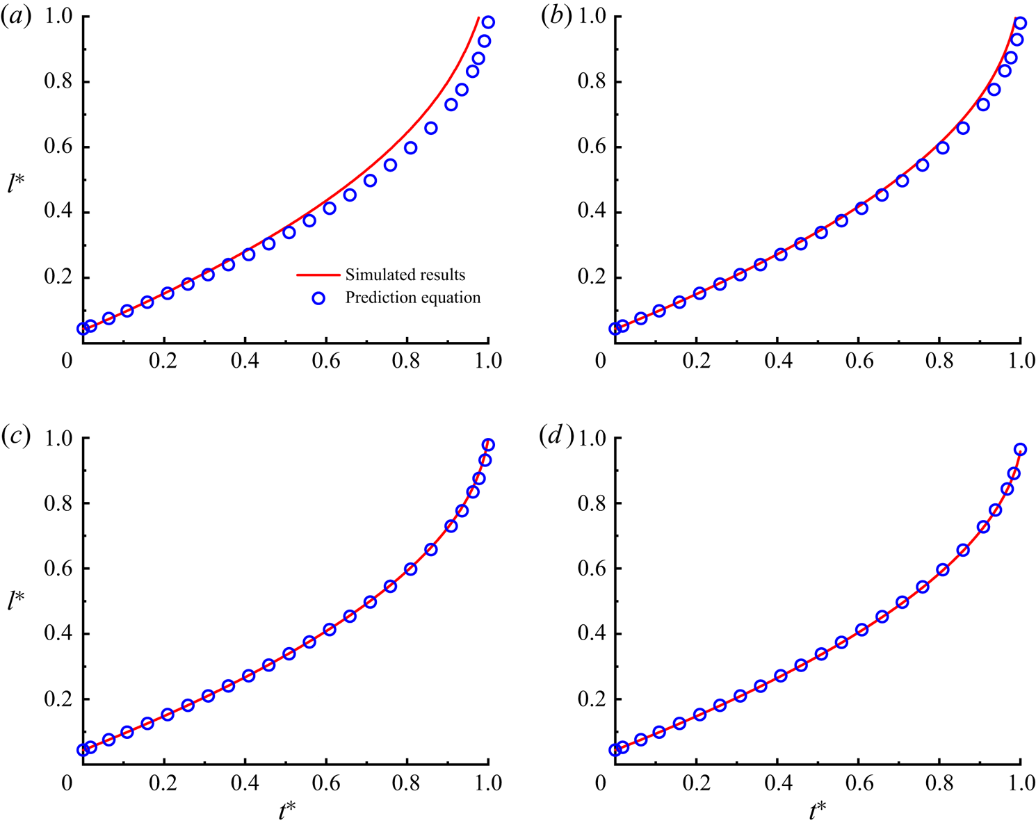
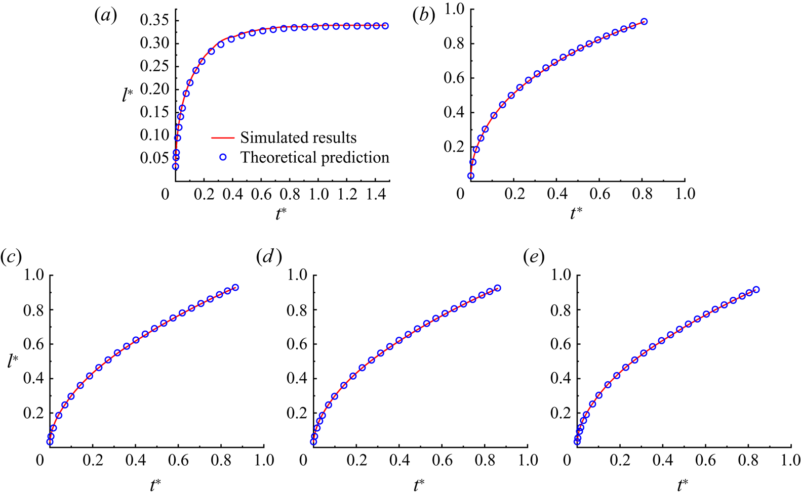
Figure 2 shows the simulated imbibition length as a function of time, where the analytical predictions from (2.8) or (2.9) are also plotted for comparison. It is seen that the evolution curves of  $l^*$ exhibit concave-up shapes for all cases. This is because the length of the non-wetting fluid column gradually decreases as the imbibition proceeds. In the condition of
 $\lambda < 1$, the viscous resistance of the system decreases with time, leading to a higher imbibition rate at a later stage. In addition, we notice that the simulated imbibition profiles agree well with the analytical predictions at
 $\varepsilon = 1/3$ and
 $1/4$. This means that the quasi-3D method can provide satisfactory simulation results only when
 $\varepsilon \leqslant 1/3$. To verify this conclusion, we also simulate the imbibition processes with
 $\varepsilon = 1/3$ for higher viscosity ratios of
 $\lambda =30$ and 50, which are realised by adjusting the value of
 $\mu _B$ but fixing
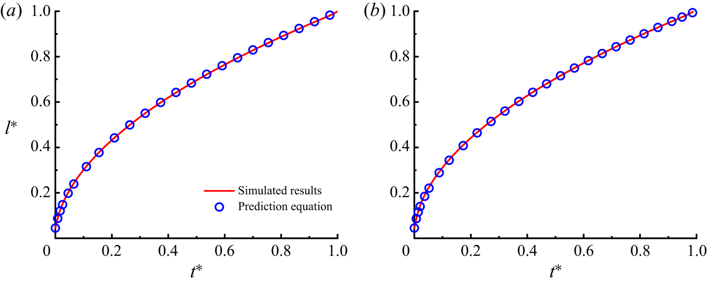
 $\mu _R=0.1$. Figure 3 shows a comparison between the simulated imbibition profiles and the analytical predictions for
 $\lambda =30$ and 50. It is seen that the imbibition profiles show concave-down shapes in the condition of
 $\lambda > 1$, which is due to the increased amount of more viscous wetting fluid resulting in an increased viscous resistance during the imbibition. As anticipated, good agreement between simulation results and analytical predictions is again observed, verifying that the quasi-3D method works well for
 $\varepsilon \leqslant 1/3$, regardless of the viscosity ratio.
The imbibition length  $l^*$ versus time
 $t^*$ at
 $\lambda =1/30$ for aspect ratios of (a)
 $\varepsilon =1$, (b)
 $\varepsilon =1/2$, (c)
 $\varepsilon =1/3$ and (d)
 $\varepsilon =1/4$. The simulation results are represented by solid lines, while the analytical predictions from (2.8) or (2.9) are represented by discrete symbols.


4.2. Spontaneous imbibition in micromodel
After obtaining the application condition of the quasi-3D method, we use it to study spontaneous imbibition in a porous media micromodel, which has a uniform depth with porosity of  $0.484$. Figure 4(a) displays the micromodel geometry in the
 $x$–
 $y$ plane, where black and grey regions represent the solid grains and the void space, respectively. The micromodel is discretised into a pore network with a grid size of
 $3000\times 4000$, and its depth is set to
 $h=5$ or
 $10$. With such a grid resolution, the narrowest flow path has a width of
 $30$, which means that the condition of
 $\varepsilon \leqslant 1/3$ can be satisfied in the whole computational domain. It is noted that the intrinsic permeability of the micromodel varies with the depth
 $h$, and its value is found to be
 $K=0.505$ for
 $h=5$ and
 $K=1.88$ for
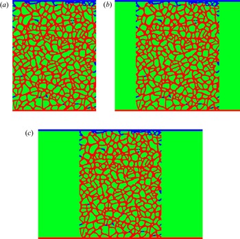
 $h=10$. To ensure that the wetting and non-wetting fluids can flow in and out continuously by using the modified periodic boundary conditions (Liu et al. Reference Liu, Sun, Wu, Wei and Hou2021), a number of layers of void nodes are added to the top and bottom sides of the pore network serving as inlet and outlet sections. For a better visualisation of the geometry set-up, we also plot the simplified diagram of the computational domain in figure 4(b), where the bottom inlet section, the middle pore network and the top outlet section can be clearly seen. To minimise the effect of the inlet (outlet) section size, we conduct a series of numerical tests with various inlet (outlet) section lengths and inlet (outlet) section widths, which are respectively denoted as
 $L_d$ and
 $W_d$ in figure 4(b). Detailed numerical results are presented in Appendix B, which shows that the inlet (outlet) section size with
 $L_d=60$ and
 $W_d=3000$ could produce reasonable outcomes and thus is used in subsequent simulations. Initially, the whole computational domain is saturated with the non-wetting fluid except the inlet section, which is occupied by the wetting fluid. In the simulations, the contact angles are kept in the range from
 $25^{\circ }$ to
 $60^{\circ }$, and most of them are not less than
 $45^{\circ }$, so the development of corner films is unfavourable. In addition, the surface tension coefficient and the viscosity of the more viscous fluid are fixed at
 $0.05$ and
 $0.2$, respectively, and the values of other parameters are specified for each case below. For each case, we run the simulation until the wetting fluid breaks through the top side of the pore network or the system reaches the steady state.
(a) The micromodel geometry and (b) the simplified diagram of the computational domain in the  $x$–
 $y$ plane. In (b), the bottom inlet section, the middle pore network and the top outlet section can be clearly seen. The void space and solid grains are indicated in grey and black, respectively. The left and right boundaries are both solid walls.

4.2.1. Low viscosity ratio
We first focus on the imbibition with a low viscosity ratio, i.e.  $\lambda =1/30$. The contact angle and the micromodel depth are set to
 $45^\circ$ and
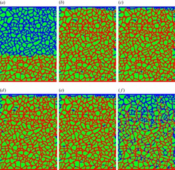
 $10$, respectively. Figure 5 shows the final fluid distributions for various values of gravitational acceleration, that is,
 $g = -5 \times 10^{-6}$,
 $-1 \times 10^{-6}$,
 $0$,
 $5 \times 10^{-6}$,
 $2.5 \times 10^{-5}$ and
 $5 \times 10^{-5}$. Recall that a negative value of
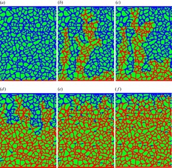
 $g$ means a downward gravitational force. It is seen that the fingering regime is identified at
 $g=0$, where preferential flow paths towards the outlet with limited or no lateral flows form in the pore network (see figure 5c). This is understandable, because once the preferential flow path of less viscous fluid is formed, it will have lower flow resistance along this path, favouring the development of a longer finger. When
 $g$ is increased from
 $-1 \times 10^{-6}$ to
 $5 \times 10^{-5}$, we can observe a significant regime shift from fingering to compact displacement, in which the front progresses forward in a nearly flat manner with very little non-wetting fluid left behind. To understand this phenomenon, we need to clarify the role of gravity in these cases. On the one hand, taking the case of
 $g=5 \times 10^{-5}$ as an example, an upward gravitational force is able to promote the imbibition process. However, it acts only on the more viscous fluid, i.e. the non-wetting defending fluid, so the promoting effect positively correlates with the amount of the non-wetting defending fluid, as can be seen from (2.5). The longer finger corresponds to less non-wetting fluid, meaning a weaker promoting effect from gravity. Therefore, the preferential flow is inhibited, and the imbibition shows a relatively compact advancing front, as shown in figures 5(e) and 5( f). On the other hand, as we decrease
 $g$ to a negative value, the gravitational force acts as a resistance for the imbibition, like the viscous force exerted on the non-wetting fluid. As a consequence, a longer finger corresponds to a lower flow resistance, leading to more pronounced fingering and thus narrower preferential flow paths, which can be seen from figure 5(b). However, once the negative gravity is large enough to counteract the effect of the capillary force, the wetting fluid would fail to displace the non-wetting fluid, and such an interesting situation is shown in figure 5(a).
Final fluid distributions in the micromodel for gravitational accelerations of (a)  $g=-5 \times 10^{-6}$, (b)
 $g=-1 \times 10^{-6}$, (c)
 $g=0$, (d)
 $g=5 \times 10^{-6}$, (e)
 $g=2.5 \times 10^{-5}$ and ( f)
 $g=5 \times 10^{-5}$. The wetting and non-wetting fluids are indicated in red and blue, respectively, while the solid grains are indicated in green. The wetting fluid is imbibed into the pore network from the bottom inlet.

When compact displacement occurs, which is of 1-D nature, we examine whether the developed theoretical model is able to predict the imbibition process. Substituting the values of  $K$,
 $\phi$ and
 $h$ into (2.13), we can obtain the equivalent width
 $w_e=11.15$ for the micromodel considered. For the sake of simplicity, the contact angle
 $\theta$ is provisionally taken as its static value of
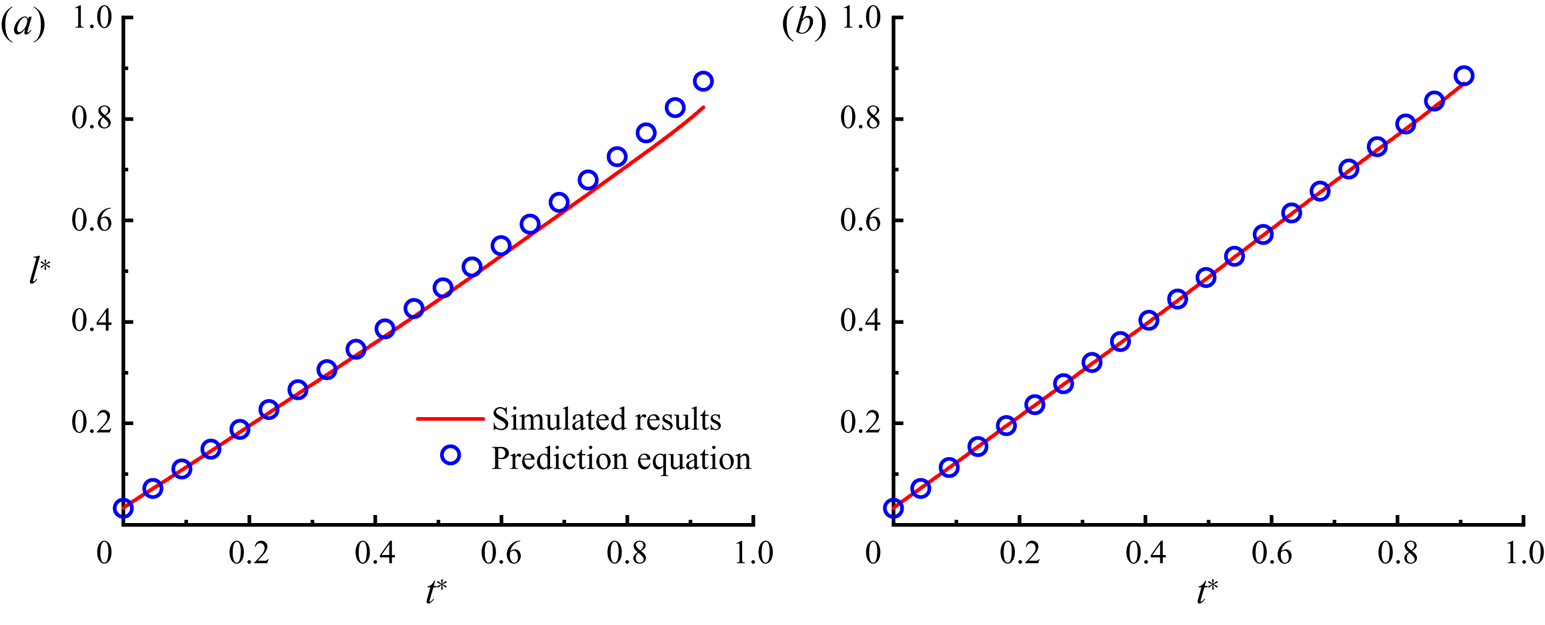
 $45^\circ$ in the prediction equation (its rationality is justified or explained in § 4.2.2). Figure 6 shows a comparison between the predicted and simulated saturations of the wetting fluid as a function of time for
 $g=2.5 \times 10^{-5}$ and
 $5 \times 10^{-5}$. It is clear that the predicted results agree well with the simulated ones except for a subtle difference at late stage, which can be explained by the imbibition patterns shown in figures 5(e) and 5( f). In the late stage of the imbibition, the advancing fronts exhibit fingering as the effect of gravity becomes less pronounced. Therefore, the prediction equation that is applicable only to the 1-D imbibition process cannot predict well the growth of
 $l^*$ in this stage. Also, the increased amount of non-wetting fluid left behind the fronts may contribute to this difference, because its influence is not able to be evaluated in the theoretical analysis. On the other hand, we notice that the evolution curve of
 $l^*$ somehow looks like a straight line, especially for
 $g=5\times 10^{-5}$. With the aid of prediction equation (2.9), we can explain this based on the force analysis. Although the gravitational force and viscous resistance exerted on the non-wetting fluid decrease as the wetting front advances, they both play a dominant role during most of the imbibition. For example, even when
 $l^*$ is as high as
 $0.6$, we can obtain the following relationships:
 \begin{equation} \frac{\rho g w_e h (L-l)}{2\sigma \cos \theta (w_e + h)} = 5.97, \quad \frac{\mu_B(L-l)}{\mu_R l} = 20, \end{equation}
where the first equation represents the ratio of the gravitational force to the capillary force and the second denotes the ratio of the viscous force exerted on the non-wetting fluid to that exerted on the wetting fluid. Therefore, in the early and middle stages of the imbibition, one can approximately write (2.9) as
 \begin{equation} \frac{{\rm d}l^*}{{\rm d}t} \approx \frac{\varepsilon \xi\left( \varepsilon\right) \left[ \rho g w_e h (1-l^*)\right]}{12\left[\mu_B(1-l^*)\right]}=\frac{\varepsilon \xi\left( \varepsilon\right) \rho g w_e h}{12\mu_B}. \end{equation}
This indicates that the saturation of the wetting fluid linearly increases with time. Also, stronger gravity can lead to a larger value of  $[ \rho g w_e h (L-l)] / [ 2\sigma \cos \theta (w_e + h)]$, and thus to a longer linear growth duration of
 $l^*$, which can be seen from a comparison between figures 6(a) and 6(b).
Time evolution of wetting fluid saturation  $l^*$ for gravitational accelerations of (a)
 $g=2.5 \times 10^{-5}$ and (b)
 $g=5 \times 10^{-5}$. The simulation results are represented by solid lines, while the analytical predictions from (2.9) are represented by discrete symbols.

4.2.2. High viscosity ratio
Next, we study spontaneous imbibition with high viscosity ratio, which is commonly encountered in natural and industrial applications (Elizalde, Urteaga & Berli Reference Elizalde, Urteaga and Berli2015; Wijshoff Reference Wijshoff2018; Wang & Zhao Reference Wang and Zhao2021). Here, the viscosity ratio is set to  $30$ or
 $50$, and various values of contact angle, micromodel depth and gravitational acceleration are considered. Unlike the cases in § 4.2.1, gravitational force is applied to the wetting fluid, which is more viscous. Figure 7 shows the fluid distributions at breakthrough or in the steady state for different groups of
 $g$ and
 $\theta$ at
 $\lambda =30$. When
 $g$ is increased from
 $-5 \times 10^{-6}$ to
 $1.25 \times 10^{-4}$ at
 $\theta =45^\circ$ (see figure 7a,b,c, f), we can identify two different imbibition regimes, namely compact displacement and fingering, which occur at
 $g\leqslant 0$ (i.e.
 $g=-5 \times 10^{-6}$,
 $-1 \times 10^{-6}$ and
 $0$) and
 $g >0$ (i.e.
 $g=1.25 \times 10^{-4}$), respectively. This can be explained as follows. An upward gravitational force (
 $g >0$) can promote imbibition, and its magnitude positively correlates with the amount of the wetting fluid, as can be seen from (2.5). Upon the onset of a preferential flow path in the pore network, a larger gravitational force would speed up the advancing front, thus favouring the development of fingering. We also notice in figure 7( f) that fingering is present in a dispersed form, similar to the viscous fingering observed in drainage experiments and simulations (Liu, Valocchi & Kang Reference Liu, Valocchi and Kang2013; Chang et al. Reference Chang, Kneafsey, Tokunaga, Wan and Nakagawa2021). By contrast, a downward gravitational force plays the same role as the viscous resistance exerted on the wetting fluid, which inhibits the development of preferential flow paths (Liu et al. Reference Liu, Sun, Wu, Wei and Hou2021). Thus, a compact advancing front would be formed, as shown in figures 7(a)–7(e). In particular, for imbibition at
 $g=-5 \times 10^{-6}$, as more wetting fluid is imbibed into the pore network, the gravitational force increases until reaching a balance with the capillary force, and the wetting front eventually stabilises at around one-third the length of the micromodel (see figure 7a).
Final fluid distributions in the micromodel for (a)  $g=-5 \times 10^{-6}$,
 $\theta =45^\circ$, (b)
 $g=-1 \times 10^{-6}$,
 $\theta =45^\circ$, (c)
 $g=0$,
 $\theta =45^\circ$, (d)
 $g=0$,
 $\theta =25^\circ$, (e)
 $g=0$,
 $\theta =60^\circ$ and ( f)
 $g=1.25 \times 10^{-4}$,
 $\theta =45^\circ$. Note that the micromodel depths are all set to
 $h=10$ except in the case (d) where
 $h=5$. The wetting and non-wetting fluids are indicated in red and blue, respectively, while the solid grains are indicated in green. The wetting fluid is imbibed into the pore network from the bottom inlet.

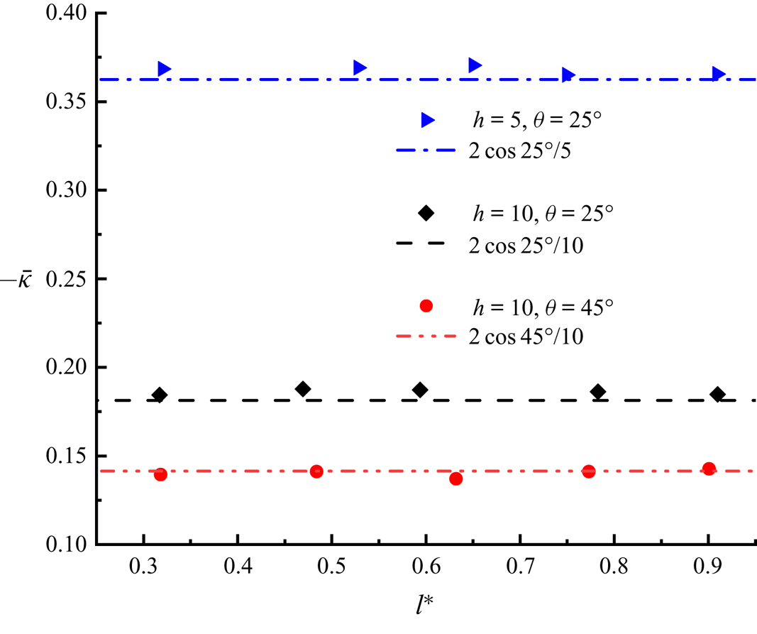
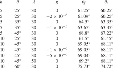
We also record the wetting fluid saturations during imbibition for 11 different cases, among which five typical cases are shown in figure 8. It is surprisingly found that the theoretical predictions with static contact angle  $\theta$ deviate considerably from the simulation results for all the cases considered, and thus we fit the simulation data using the prediction equation with an adjustable contact angle but all the other parameters following their original definitions. The fitting contact angles for all cases are listed in table 1. Recall that in the previous theoretical derivation, the contact angle appears only to estimate the interface curvature involved in the capillary force. Therefore, we turn to monitoring the variation of the mean interface curvature during imbibition, where the mean interface curvature
 $\bar {\kappa }$ is computed by averaging all the interface curvatures
 $\kappa$ at the advancing front. As examples, figure 9 plots
 $-\bar {\kappa }$ against the wetting fluid saturation
 $l^*$ for three groups of
 $h$ and
 $\theta$ at
 $g=0$ and
 $\lambda =30$. It is seen that the values of
 $-\bar {\kappa }$ approximately equal
 $2\cos \theta /h$ during imbibition, which means that the mean interface curvature in the
 $x$–
 $y$ plane is so small that it can be ignored. (Theoretically,
 $-\bar {\kappa } = -\bar {\kappa }_{xy} + 2\cos \theta /h$, where
 $\bar {\kappa }_{xy}$ is the mean interface curvature in the
 $x$–
 $y$ plane and
 $-2\cos \theta /h$ is the depth-oriented interface curvature.) To clarify the cause of
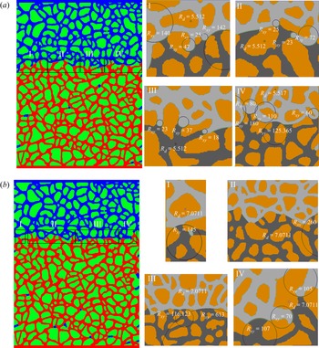
 $\bar {\kappa }_{xy}\approx 0$, we take a closer look at local fluid distributions extracted from the instantaneous results at
 $l^*=0.59$ for
 $h=10$ and
 $\theta =25^\circ$, and at
 $l^*=0.63$ for
 $h=10$ and
 $\theta =45^\circ$, which are displayed in figure 10. We can see that the advancing front frequently flows through intersections of different flow paths, which gives a relatively large curvature radius (
 $R_{xy}$) and thus a small value of interface curvature in the
 $x$–
 $y$ plane. In addition, the frequently encountered capillary valve resistance, which occurs when the advancing front undergoes a sudden geometry expansion, also reduces the mean interface curvature
 $\bar {\kappa }_{xy}$. This is because the front shows a convex shape in the capillary valve structure (Wu et al. Reference Wu, Kharaghani and Tsotsas2016; Xu et al. Reference Xu, Liu and Valocchi2017), and the resulting interface curvature would counteract the curvature created by the concave interface in the throat. However, the depth-oriented interface curvature would not be influenced by these local structures, since the entire micromodel has a uniform depth. Based on the above discussion, we can define an equivalent contact angle
 $\theta _e$ as
 \begin{equation} \frac{2 \cos \theta_e}{h} + \frac{2 \cos \theta_e}{w_e} = \frac{2 \cos \theta}{h}, \end{equation}
where  $\theta$ is the static contact angle specified as an input parameter in the simulation. Obviously, the equivalent contact angle would coincide with the static contact angle for a sufficiently low ratio of the height
 $h$ to the equivalent width
 $w_e$. It is worth emphasising that in the prediction equations of the micromodel, the equivalent contact angle
 $\theta _e$ should be used instead of the static one in order to exclude the capillary force in the
 $x$–
 $y$ plane. Table 1 also presents the predicted
 $\theta _e$ values from (4.3). It is seen that the fitting contact angles match well with the predicted ones, with the largest deviation of
 $1.58^{\circ }$, validating our theoretical derivations for micromodels. In principle, the developed prediction equations, i.e. (2.8), (2.13) and (4.3), can be applied for the quantification of contact angle in micromodels, where direct measurement is often a difficult task (Blunt et al. Reference Blunt, Lin, Akai and Bijeljic2019; Sun et al. Reference Sun, McClure, Mostaghimi, Herring, Berg and Armstrong2020). In addition, we find that at
 $h=10$,
 $\theta =45^\circ$ and
 $g=0$, the results of
 $\lambda =30$ and
 $\lambda =50$ are almost the same, consistent with the previous finding that the viscosity of non-wetting fluid has a negligible influence on the imbibition for
 $\lambda \geqslant 30$ (Liu et al. Reference Liu, Sun, Wu, Wei and Hou2021). We also examine the flow regimes for the imbibition cases shown in table 1. To start with, we define the Reynolds number as
 \begin{equation} Re = \frac{\rho U_f L_c}{\mu_c}, \end{equation}
where  $U_f$ is the mean velocity of wetting front and
 $\mu _c$ is the characteristic viscosity. Length
 $L_c$ is the characteristic length, and it is selected as the width of the flow channel or the hydraulic diameter
 $D = 2 h w / (h + w)$, in which
 $w$ is the width of the flow channel (Zacharoudiou et al. Reference Zacharoudiou, Chapman, Boek and Crawshaw2017). Strictly speaking, the imbibition process includes two stages, namely the very early stage and the mid-to-late stage. In the mid-to-late stage, a sufficient amount of more viscous wetting fluid has been imbibed into the micromodel, so the viscosity of wetting fluid plays a dominant role. Accordingly, we choose the viscosity of wetting fluid as the characteristic viscosity. In the simulations, the mean velocity of the wetting front is usually of the order of
 $10^{-4}$ or less, and the density, length scale and viscosity are usually of the orders of
 $10^0$,
 $10{^1}$ and
 $10^{-1}$, respectively (all the quantities are shown in lattice units here). Thus, the resulting Reynolds number is
 $Re \sim 10^{-2}$, which means that fluid flows through the micromodel are typically in the Stokes regime. In the very early stage, the less viscous non-wetting fluid almost occupies the entire micromodel, and thus its viscous pressure drop will dominate the imbibition process, which means that the characteristic viscosity in
 $Re$ should be the viscosity of non-wetting fluid. In this condition, if the viscosity of non-wetting fluid is extremely low, the Reynolds number will be high. Therefore, the very early stage is often called the ‘inertial regime’, where the Stokes flow condition does not hold. However, previous studies showed that this stage is too short to have a visible influence on the entire imbibition process (Zacharoudiou et al. Reference Zacharoudiou, Chapman, Boek and Crawshaw2017; Liu et al. Reference Liu, Sun, Wu, Wei and Hou2021; Ruiz-Gutiérrez et al. Reference Ruiz-Gutiérrez, Armstrong, Lévêque, Michel, Pagonabarraga, Wells, Hernández-Machado and Ledesma-Aguilar2022). To demonstrate this, we consider a typical case with viscosity ratio of 30, static contact angle of
 $45^\circ$ and gravitational acceleration of 0, and the results are displayed in figure 8(c). According to (2.3), the competition between the viscous pressure drops across the wetting and non-wetting fluids can be expressed as
 \begin{equation} \lambda_f = \frac{\mu_R l}{\mu_B(L-l)}. \end{equation}
It is clear that when  $\lambda _f>3$, the viscous pressure drop across the wetting fluid will play a dominant role, meaning that the imbibition has entered the mid-to-late stage. Substituting
 $\mu _R / \mu _B=30$ and
 $\lambda _f>3$ into (4.5), we have
 $l^* =l/L> 1/11$. Using the data shown in figure 8(c), it is found that the corresponding dimensionless time is
 $t^*>0.0083$. This suggests that the very early stage lasts at most until
 $t^* =0.0083$, which is extremely short for the entire duration of imbibition. Therefore, we conclude that the Stokes flow condition can be well satisfied in the entire process of spontaneous imbibition. It is also worth noting that the Stokes flow means the front motion happens on a time scale
 $\tau _f$ (
 $\tau _f = L_c / U_f$) much slower than the time scale
 $\tau _\nu$ (
 $\tau _\nu = \rho L^2_c / \mu _c$) for a viscous flow to reach steady state. Thus, the quasi-static assumption made in the derivation of the theoretical model (see § 2) does hold in our simulations.
Time evolution of wetting fluid saturation  $l^*$ for (a)
 $g=-5 \times 10^{-6}$,
 $\theta =45^\circ$, (b)
 $g=-1 \times 10^{-6}$,
 $\theta =45^\circ$, (c)
 $g=0$,
 $\theta =45^\circ$, (d)
 $g=0$,
 $\theta =25^\circ$ and (e)
 $g=0$,
 $\theta =60^\circ$. Note that the micromodel depth is set to
 $h=10$ in all cases except in (d) where
 $h=5$. In these cases, the predicted curves are obtained using the fitting contact angles, and their values are given in table 1.

Plots of  $-\bar {\kappa }$ versus
 $l^*$ during imbibition for different groups of
 $h$ and
 $\theta$ at
 $g=0$ and
 $\lambda =30$. Note that the values of
 $2\cos \theta /h$ are also plotted as straight lines for comparison.

The instantaneous fluid distributions at (a)  $l^*=0.59$ for
 $h=10$ and
 $\theta =25^ \circ$ and (b)
 $l^*=0.63$ for
 $h=10$ and
 $\theta =45^ \circ$. In each case, the right-hand panels show close-ups of the front regions where the circles with radii
 $R_{xy}$ are added to highlight the interface curvatures in the
 $x$–
 $y$ plane, while the circle with radius
 $R_{d}$ is plotted to show the interface curvature in the depth direction.

Comparison between the fitting contact angle  $\theta _f$ and the theoretical value
 $\theta _e$ in various cases. Note that in each case,
 $\theta _f$ is obtained by fitting the simulated results with (2.8).

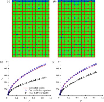
The above studies are carried out on the basis of irregular geometries, while regular geometries composed of orderly pores and throats are also encountered quite often in both experimental and numerical researches (Corapcioglu, Chowdhury & Roosevelt Reference Corapcioglu, Chowdhury and Roosevelt1997; Sun et al. Reference Sun, Kharaghani and Tsotsas2016; Wu et al. Reference Wu, Kharaghani and Tsotsas2016; Gasow et al. Reference Gasow, Kuznetsov, Avila and Jin2021; Xie et al. Reference Xie, Lei, Balhoff, Wang and Chen2021; Yang et al. Reference Yang, Fu, Du, Xu, Balhoff, Weston and Lu2021). To examine whether the developed prediction equations are general enough to describe various geometries, we investigate imbibition in a regular micromodel. The micromodel has a uniform depth of  $10$, and its 2-D pore network, which has a size of
 $3070\times 4715$, consists of square pores connected by rectangular throats. The intrinsic permeability and porosity of the micromodel are
 $1.2797$ and
 $0.3251$, respectively. With these parameters, we are able to solve the equivalent width of the micromodel,
 $w_e=11.32$, and the equivalent contact angles
 $\theta _e=62.62^\circ$ and
 $67.94^\circ$ for
 $\theta =30^\circ$ and
 $45^\circ$, respectively. The simulations are run with
 $\mu _R=0.2$,
 $\lambda =30$ and
 $\sigma =0.05$, and two different cases are considered: one with
 $\theta =45^\circ$ and
 $g=0$ and the other with
 $\theta =30^\circ$ and
 $g=-5\times 10^{-7}$. Figure 11 shows the fluid distributions at breakthrough and the evolution curves of
 $l^*$ for these two cases. As expected, the wetting front progresses forward in a nearly flat manner, which thus allows us to predict the imbibition processes using the developed equation (2.8) with
 $w_s$ and
 $\theta$ replaced by
 $w_e$ and
 $\theta _e$. In figures 11(c) and 11(d), in addition to our predicted results, we also plot the results obtained from the prediction equation of Fries & Dreyer (Reference Fries and Dreyer2008), which has been commonly used to model the capillary rise of liquids in porous media. It is seen that our theoretical predictions agree well with the simulated results, while the theoretical predictions from Fries & Dreyer (Reference Fries and Dreyer2008) deviate a lot from the simulated results. This difference can be explained as follows: Fries & Dreyer (Reference Fries and Dreyer2008) derived the prediction equation on the basis of the cylindrical tube assumption, and the key geometrical characteristics of the micromodel were thus ignored in their derivation. For example, in the micromodel, which consists of flow channels with rectangular cross-section, the mathematical expression of viscous resistance is totally different from that of a cylindrical tube (Ouali et al. Reference Ouali, McHale, Javed, Trabi, Shirtcliffe and Newton2013). In addition, as shown above, the depth-oriented interface curvature completely determines the capillary force of the advancing front in the micromodel, which should be taken into consideration when deriving the prediction equation. We also note that, for the theoretical predictions shown in figure 6, the deviation caused by inaccurate contact angle is not pronounced (see the comparison between the results from the prediction equation with static contact angle and from the prediction equation with equivalent contact angle in figure 12), which is because the imbibition is primarily driven by gravity rather than by the capillary force. This also explains why the predicted results are closer to the simulated ones for
 $g=5 \times 10^{-5}$ than for
 $g=2.5 \times 10^{-5}$ in figure 6.
The fluid distributions at breakthrough and wetting fluid saturation  $l^*$ versus time
 $t^*$ for (a,c)
 $\theta =45^\circ$ and
 $g=0$ and (b,d)
 $\theta =30^\circ$ and
 $g=-5 \times 10^{-7}$. In (c,d), the circles represent the theoretical predictions from (2.8) where
 $w_s$ and
 $\theta$ should be replaced by
 $w_e$ and
 $\theta _e$, while the triangles represent the theoretical predictions from Fries & Dreyer (Reference Fries and Dreyer2008).

Time evolution of wetting fluid saturation  $l^*$ for gravitational accelerations of (a)
 $g=2.5 \times 10^{-5}$ and (b)
 $g=5 \times 10^{-5}$. The simulation results are represented by solid lines, while the analytical predictions from (2.9) with static contact angle
 $\theta$ and with equivalent contact angle
 $\theta _e$ are represented by discrete circles and triangles, respectively.

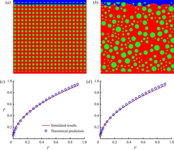
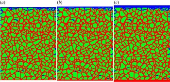
Finally, to show the generality of the proposed model, we investigate spontaneous imbibition in three more micromodels, namely the homogeneous micromodel, the heterogeneous micromodel and the VORONOI-like micromodel. Figures 13(a) and 13(b) show the homogeneous and heterogeneous micromodel geometries in the  $x$–
 $y$ plane, both of which are discretised into a
 $2000 \times 2000$ computational domain, and the depths are set to 10. The homogeneous micromodel is composed of uniformly distributed circular grains with a diameter of 60, and the centre distance between two neighbouring grains is 100. In this condition, the intrinsic permeability and porosity of the homogeneous micromodel are found to be 4.17 and 0.7379, respectively. The heterogeneous micromodel consists of randomly distributed circular grains, with the smallest grain diameter of 30 and the largest grain diameter of 150. To ensure sufficient computing accuracy, we assign 30 lattices for the narrowest channel inside the pore space, while the widest channel has a width of 500, which is around 16.7 times the width of the narrowest channel. The intrinsic permeability and porosity are 4.33 and 0.7422, which are close to those of the homogeneous micromodel. We run the simulations with a viscosity ratio of
 $\lambda = 30$, static contact angle of
 $\theta = 60^\circ$ and gravitational acceleration of
 $g = 0$ for these two geometries. Figures 13(a) and 13(b) show the final fluid distributions in the homogeneous and heterogeneous micromodels. As we expect, the imbibitions in both geometries exhibit compact displacement patterns, so we can use the proposed theoretical model to predict the imbibition processes. According to the simulation parameters used, the equivalent widths and contact angles can be calculated, and their values are
 $w_e=18.98$ and
 $\theta _e=70.89^\circ$ for the homogeneous micromodel and
 $w_e=20.2$ and
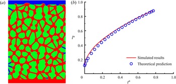
 $\theta _e=70.5^\circ$ for the heterogeneous micromodel. Figures 13(c) and 13(d) show a comparison between the predicted and simulated results, and good agreements are obtained in both micromodels. This indicates that the proposed theoretical model can provide satisfactory prediction of spontaneous imbibition in the micromodels with homogeneous or heterogeneous geometries. Then, we consider spontaneous imbibition in the VORONOI-like micromodel. As shown in figure 14(a), the randomly distributed throats with widths of 30 and circular pores with diameters of 76 constitute the pore space. The micromodel has a size of
 $1426 \times 2052$ in the
 $x$–
 $y$ plane, and its depth is 10. The intrinsic permeability and porosity of the micromodel are 1.68 and 0.4583, respectively. In the simulation, we again choose the viscosity ratio as
 $30$, so that imbibition occurs in the compact displacement regime. The static contact angle and gravitational acceleration are set to
 $46^\circ$ and
 $0$, respectively. With these parameters, we compute the equivalent width and contact angle, and their values are
 $w_e=10.52$ and
 $\theta _e=69.14^\circ$. The fluid distribution at breakthrough is shown in figure 14(a), where we observe the wetting front advancing upward in a flat manner. Figure 14(b) plots the wetting fluid saturation versus the dimensionless time, in which the predicted values from the theoretical model are also shown for comparison. Obviously, the simulated results match fairly well with the predicted values. Based on the results shown above, we conclude that the proposed model is general enough to provide accurate prediction of spontaneous imbibition in various micromodels.
The fluid distributions at breakthrough and wetting fluid saturation  $l^*$ versus the dimensionless time
 $t^*$ in (a,c) the homogeneous micromodel and (b,d) the heterogeneous micromodel.

(a) The fluid distributions at breakthrough and (b) wetting fluid saturation  $l^*$ versus the dimensionless time
 $t^*$ for spontaneous imbibition in the VORONOI-like micromodel.

4.3. Quantitative comparison with experiment
In this section, we conduct an experiment on absolute ethanol spontaneously imbibed into a vertically placed micromodel to displace in situ air, and the obtained results are used to further verify the quasi-3D simulations and the developed prediction equation. To allow for a direct visualisation of the advancing front, we choose transparent polydimethylsiloxane material to fabricate the micromodel, which has a size of  $57.2\ {\rm mm} \times 58.2\ {\rm mm} \times 50\ \mathrm {\mu }{\rm m}$. The micromodel pattern is represented by a 2-D pore network in which void space consists of square pores with side length of
 $1$ mm, and interconnected rectangular throats with widths uniformly distributed from 0.194 to 0.795 mm (for more details on the pore network geometry, interested readers are referred to https://github.com/file-cloud-world/geometry). The porosity and intrinsic permeability of the micromodel are
 $0.5236$ and
 $6.2073 \times 10^{-11}\ {\rm m}^2$, respectively. The micromodel experiment is carried out at room temperature (
 $25\,^{\circ }\mathrm {C}$) with gravitational acceleration of
 $-9.81\ {\rm m}\ {\rm s}^{-2}$. In this condition, the dynamic viscosities of the wetting and non-wetting fluids are
 $1.013 \times 10^{-3}$ and
 $1.8523 \times 10^{-5}\ {\rm Pa}\ {\rm s}$, respectively, and their surface tension is
 $2.197 \times 10^{-2}\ {\rm N}\ {\rm m}^{-1}$. The measured contact angle is around
 $55^\circ$, and detailed information on the micromodel experiment and measurement can be found in Wu et al. (Reference Wu, Zhang, Ye, Zhao, Tsotsas and Kharaghani2020). According to these parameters, we can compute the equivalent width and equivalent contact angle of the micromodel, and their values are
 $w_e=7.1236 \times 10^{-5}$ m and
 $\theta _e=70.3^\circ$, respectively. The LBM simulation is conducted in the lattice space, and we can map the physical parameters to the lattice space by using three reference scales: the length scale
 $L_0=9.7 \times 10 ^{-6}$ m, the time scale
 $T_0=1.516 \times 10 ^{-6}$ s and the mass scale
 $M_0=7.21 \times 10 ^{-13}$ kg. Specifically, a physical parameter with dimensions
 $[ \text {m}]^{n_1} [ \text {s}]^{n_2} [ \text {kg}]^{n_3}$ is divided by
 $[ L_0]^{n_1} [ T_0]^{n_2} [ M_0]^{n_3}$ to obtain its corresponding LBM parameter (Liu & Zhang Reference Liu and Zhang2017; Li et al. Reference Li, Liu, Zhang, Jiang and Xi2021). Following this criterion, we can obtain, for example, the LBM value of the viscosity
 $\mu _R^{phy}$ by
 \begin{equation} \mu_R=\mu_R^{phy}\left/ \left(\frac{M_0}{L_0 T_0}\right)\right. =1.013 \times 10^{{-}3}\frac{( 9.7 \times 10 ^{{-}6}) ( 1.516 \times 10 ^{{-}6}) }{7.21 \times 10 ^{{-}13}} =0.021, \end{equation}
the LBM value of the gravity acceleration  $g^{phy}$ by
 \begin{equation} g=g^{phy}\left/ \left(\frac{L_0}{T_0^2}\right)\right. ={-}9.81\frac{( 1.516 \times 10 ^{{-}6})^2 }{9.7 \times 10 ^{{-}6}} ={-}2.324\times 10^{{-}6} \end{equation}
and the LBM value of the surface tension coefficient  $\sigma ^{phy}$ by
 \begin{equation} \sigma=\sigma^{phy}\left/ \left(\frac{M_0}{T_0^2}\right)\right.=2.197\times 10^{{-}2}\frac{( 1.516 \times 10 ^{{-}6})^2 }{7.21 \times 10 ^{{-}13}} =0.07, \end{equation}
where the superscript ‘ $phy$’ represents the physical parameter and it is added to distinguish from the LBM parameter. Initially, the vertical placed micromodel is fully saturated with air, and its bottom side is just in touch with the absolute ethanol. Driven by the capillary force, the interface advances upward as the experiment proceeds, and the height of the front is recorded as a function of time.
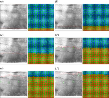
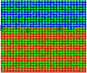
Figure 15 shows a comparison of the fluid distributions obtained from experiment (left-hand half of each panel) and simulation (right-hand half of each panel) for several typical moments during the imbibition. As expected, the imbibition occurs in the compact displacement regime due to the combined effect of favourable viscosity ratio ( $\lambda >1$) and downward gravity. In the early to middle stages, the simulated wetting fronts are close to the corresponding experimental results, as shown in figure 15(a–c). As the wetting front advances, small discrepancies start to appear in figure 15(d), where the imbibition height is a little lower in the simulation. This may be due to that (1) some 3-D effects, such as wetting fluid stretching along corners (Zhao, MacMinn & Juanes Reference Zhao, MacMinn and Juanes2016; Hu et al. Reference Hu, Wan, Yang, Chen and Tokunaga2018; Zhao et al. Reference Zhao2019; Golmohammadi et al. Reference Golmohammadi, Ding, Kuechler, Reuter, Schlueter, Amro and Geistlinger2021; Zhao et al. Reference Zhao, Qin, Fischer, Kang, Derome and Carmeliet2021), thin film along the surface (Lukyanov et al. Reference Lukyanov, Sushchikh, Baines and Theofanous2012) and the wetting transition (Odier et al. Reference Odier, Levaché, Santanach-Carreras and Bartolo2017; Zhao et al. Reference Zhao, Pahlavan, Cueto-Felgueroso and Juanes2018), are not taken into consideration in the quasi-3D simulation; and/or (2) the micromodel used in the experiment may not be perfect in terms of wall smoothness and uniform wetting properties, which causes the necessity of including contact angle hysteresis (Xu et al. Reference Xu, Liu and Valocchi2017; Qin et al. Reference Qin, Zhao, Kang, Derome and Carmeliet2021). In spite of the discrepancies, the simulated results overall match well with the experimental ones, which can be also seen in figure 16. In addition, we notice that some trapped blobs observed in experiment are exactly reproduced by the present simulation; see, for example, those highlighted by the green boxes in figure 15(d–f). These agreements indicate that the quasi-3D simulations can capture essential flow physics underlying spontaneous imbibition in a micromodel, thus serving as a promising alternative to direct 3-D simulations, which are not affordable with our available computational resources. For example, it takes 222.5 GPU hours to simulate the present experiment in a
 $5900 \times 6000$ 2-D domain for the quasi-3D simulation, while direct 3-D simulation requires a least 10 times longer computational time and 10 times more memory consumption. Finally, we predict the imbibition height against time using the developed equation (2.8), and the predicted results are also presented in figure 16. It is seen that the predicted results agree well with the experimental data during the whole imbibition process, suggesting that our prediction equation can provide satisfactory predictions of the imbibition experiment.
Comparison between experimental (a,c,e) and simulated (b,d, f) fluid distributions at (a)  $t=0.76$ s, (b)
 $t=1.54$ s, (c)
 $t=7.12$ s, (d)
 $t=19.86$ s, (e)
 $t=42.28$ s and ( f)
 $t=65.0$ s. Some small boxes are included to show the trapped blobs in both experiment and simulation. For the experimental results, the fronts are highlighted by red lines.

The imbibition height as a function of time obtained from experiment, theoretical prediction and quasi-3D simulation.

5. Conclusions
In this work, we have conducted mathematical modelling and simulation of spontaneous imbibition including gravity in rectangular capillaries and porous media micromodels. By establishing the force balance of the imbibition system, we derive the mathematical model for predicting the imbibition length as a function of time in a single rectangular capillary. We also extend the developed prediction equation to the prediction of compact displacement in a micromodel using an equivalent width  $w_e$, which is derived by the analogy of a micromodel into a rectangular capillary. Then, a recently developed quasi-3D LBM is applied to simulate spontaneous imbibition in rectangular capillaries with various aspect ratios (
 $\varepsilon$), and the obtained results when compared with theoretical predictions show that the application condition of the quasi-3D LBM is
 $\varepsilon \leqslant 1/3$. Next, it is used to study spontaneous imbibition in micromodels with various geometries and flow conditions. Results show that the imbibition pattern is heavily dependent on the gravitational acceleration
 $g$. At low viscosity ratios, e.g.
 $\lambda =1/30$, we find that imbibition undergoes a regime transition from fingering to compact displacement as
 $g$ increases from negative to positive values. At high viscosity ratios, e.g.
 $\lambda =30$, the imbibition exhibits a fingering pattern when
 $g \gg 0$ but compact displacement occurs when
 $g \leqslant 0$. It is also found that during imbibition, the capillary effect of the advancing front is primarily determined by the depth-oriented interface curvature. Taking this into consideration, we introduce an equivalent contact angle
 $\theta _e$ into the prediction equation so that the capillary driving force can be appropriately evaluated. With the aid of
 $\theta _e$, the mathematical model is shown to be highly predictive of the compact displacement process in micromodels with various geometries and flow conditions. Finally, we present a micromodel experiment using absolute ethanol imbibed into a vertically placed micromodel to displace the air, and further verify the developed mathematical model and the quasi-3D simulation by reproducing the experimental results.
Funding
This work is supported by Open Fund (PLC20210309) of State Key Laboratory of Oil and Gas Reservoir Geology and Exploitation (Chengdu University of Technology), the National Natural Science Foundation of China (nos. 12072257 and 51876170), the National Key Project (no. GJXM92579) and the Major Special Science and Technology Project of the Inner Mongolia Autonomous Region (no. 2020ZD0022).
Declaration of interests
The authors report no conflict of interest.
Appendix A. Quasi-3D colour-gradient LBM and boundary conditions
Numerical simulation of spontaneous imbibition in a porous media micromodel has to account for 3-D effects, because the capillary force originating from the depth-oriented curvature is needed to overcome the capillary valve resistance, which is caused by the pore-throat structure in the horizontal plane. However, direct 3-D simulation of spontaneous imbibition in a micromodel is a great challenge since it requires a very large number of grids to correctly capture the interface curvature in the direction of micromodel depth, which is usually much smaller than the narrowest throat in the horizontal plane. To tackle this challenge, Liu et al. (Reference Liu, Sun, Wu, Wei and Hou2021) recently proposed a quasi-3D colour-gradient LBM for the simulation of two-phase flows in the micromodel, which only incurs 2-D computational cost but considers essential 3-D effects, including the depth-oriented curvature and viscous resistance from the top and bottom walls.
In the quasi-3D colour-gradient LBM, two distribution functions, namely  $f_{\alpha }^R$ and
 $f_{\alpha }^B$, are introduced to represent the immiscible red and blue fluids, respectively. Each of the distribution functions experiences collision and streaming steps expressed as
 \begin{equation} f_\alpha^{k} ({{\boldsymbol{x}}+\boldsymbol{e}_\alpha\delta_t,t+\delta_t}) = f_\alpha^k ( {{\boldsymbol{x}},t} ) + ( \varOmega_\alpha^k)^ {\left(3 \right)} [( \varOmega_\alpha^k)^ {(1)} +(\varOmega_\alpha^k)^{(2)}], \quad k=R \ \text{or} \ B, \end{equation}
where  $\delta _t =1$ is the lattice time step,
 $\boldsymbol {e}_{\alpha }$ is the lattice velocity in the
 $\alpha$th direction,
 $f_\alpha ^k( {{\boldsymbol {x}},t} )$ is the distribution function along
 $\boldsymbol {e}_{\alpha }$ at position
 $\boldsymbol {x}$ and time
 $t$, and
 $( \varOmega _\alpha ^k )^ {(1 )}$,
 $( \varOmega _\alpha ^k )^ {(2 )}$ and
 $( \varOmega _\alpha ^k )^ {(3 )}$ are the single-phase collision, perturbation and recolouring operators, respectively. For the 2-D nine-velocity (D2Q9) lattice model used in the present method, the lattice velocity
 $\boldsymbol {e}_{\alpha }$ reads as
 \begin{equation} \left[\begin{array}{@{}cccc@{}} \boldsymbol{e}_{1}, & \boldsymbol{e}_{2}, & \ldots, & \boldsymbol{e}_{8} \end{array}\right]= \begin{bmatrix} 0 & 1 & 0 & -1 & 0 & 1 & -1 & -1 & 1 \\ 0 & 0 & 1 & 0 & -1 & 1 & 1 & -1 & -1 \end{bmatrix}. \end{equation}
For simplicity, we assume that both red and blue fluids are of equal density, which allows us to implement the single-phase collision operator via the total distribution function, which is defined as  $f_{\alpha }=f_{\alpha }^R+f_{\alpha }^B$. With the multiple-relaxation-time collision model, the single-phase collision operator is given by (Ginzburg & d'Humières Reference Ginzburg and d'Humières2003)
 \begin{equation} \left( \varOmega_\alpha \right)^ {\left(1 \right)}={-}\sum_{\beta}( \boldsymbol{M}^{{-}1}\boldsymbol{S}\boldsymbol{M})_{\alpha\beta}( f_{\beta} - f_{\beta}^{eq}), \end{equation}
where  $f_{\alpha }^{eq}$ is the equilibrium distribution function, it being related to the depth-averaged velocity
 $\boldsymbol {u}$ and the total density
 $\rho$ by
 \begin{equation} f_{\alpha}^{eq}=\rho w_\alpha\left[1+\frac{{\boldsymbol{e}}_\alpha\boldsymbol{\cdot} {\boldsymbol{u}}}{c_s^2}+\frac{({\boldsymbol{e}}_\alpha\boldsymbol{\cdot} {\boldsymbol{u}})^2}{2c_s^4}-\frac{{\boldsymbol{u}}^2}{2c_s^2}\right]. \end{equation}
Herein,  $c_s=1/\sqrt {3}$ is the speed of sound and
 $w_\alpha$ is the weight factor, given as
 $w_0=4/9$,
 $w_{1-4}=1/9$ and
 $w_{5-8}=1/36$. The transformation matrix
 $\boldsymbol {M}$ is to map the distribution functions onto the moment space, and its explicit expression can be found in Lallemand & Luo (Reference Lallemand and Luo2000). Matrix
 $\boldsymbol {S}$ is the diagonal relaxation matrix, given by
 $\boldsymbol {S}=\mathrm {diag}[1.0,1.0,1.0,1.0,1.0,1.0,1.0,\omega,\omega ]$, where
 $\omega$ is related to the dynamic viscosity
 $\mu$ of the fluid mixture by
 $\mu =\rho c_s^2(1/\omega -0.5)\delta _t$ (Ginzburg & d'Humières Reference Ginzburg and d'Humières2003; Fei & Luo Reference Fei and Luo2017). To account for different viscosities of two fluids, a harmonic mean is adopted to determine the dynamic viscosity
 $\mu$, given by (Liu et al. Reference Liu, Ba, Wu, Li, Xi and Zhang2018)
 \begin{equation} \frac{1}{\mu}=\frac{1+\rho^N}{2\mu_R}+\frac{1-\rho^N}{2\mu_B}, \end{equation}
where  $\mu _R$ and
 $\mu _B$ are the dynamic viscosities of pure red and blue fluids, respectively. Function
 $\rho ^N$ is the colour function introduced to distinguish different fluids and is defined as
 \begin{equation} \rho^N({\boldsymbol{x}}, t) = \frac{\rho^R({\boldsymbol{x}}, t) - \rho^B({\boldsymbol{x}}, t)}{\rho^R({\boldsymbol{x}}, t) + \rho^B({\boldsymbol{x}}, t)}, \end{equation}
where  $\rho ^R({\boldsymbol {x}}, t)=\sum _{\alpha }f_{\alpha }^R({\boldsymbol {x}}, t)$ and
 $\rho ^B({\boldsymbol {x}}, t)=\sum _{\alpha }f_{\alpha }^B({\boldsymbol {x}}, t)$ are the local densities of red and blue fluids, respectively. It is clear that
 $\rho ^N$ ranges from
 $-1$ to
 $1$, with
 $\rho ^N=1$ and
 $\rho ^N=-1$ representing the pure red and blue fluids, respectively.
As stated above, two important 3-D effects are considered in the present method, namely the viscous resistance from the top and bottom walls and the depth-oriented interface curvature. The former can be realised by adding a force term
 \begin{equation} \boldsymbol{F}_v ={-}\frac{\mu}{K}\boldsymbol{u} \end{equation}
to the momentum equations, where  $K=h^2/12$ is the equivalent permeability in the depth direction (Horgue et al. Reference Horgue, Augier, Duru, Prat and Quintard2013), while the latter can be analytically expressed through the contact angle
 $\theta$ and the channel or micromodel depth
 $h$ as (Yin et al. Reference Yin, Zarikos, Karadimitriou, Raoof and Hassanizadeh2019)
 \begin{equation} C_d ={-}\frac{2\cos\theta}{h}. \end{equation}
Then, the perturbation operator, which is to realise the capillary and 3-D effects, can be defined as (Yu & Fan Reference Yu and Fan2010)
 \begin{equation} (\varOmega_\alpha^k)^{(2)}={\boldsymbol{M}}^{{-}1}(\boldsymbol{I}-\tfrac{1}{2}\boldsymbol{S}) \boldsymbol{M}\tilde{\boldsymbol{F}}, \end{equation}
where  $\boldsymbol {I}$ is a
 $9\times 9$ unit matrix and
 $\tilde {\boldsymbol {F}}=[ \tilde {F}_0,\tilde {F}_1,\tilde {F}_2,\ldots,\tilde {F}_{9}] ^{\rm T}$ is given by (Guo, Zheng & Shi Reference Guo, Zheng and Shi2002)
 \begin{equation} \tilde{F}_\alpha=w_\alpha\left[ \frac{\boldsymbol{e}_\alpha-\boldsymbol{u}}{c_s^{2}}+\frac{\left( \boldsymbol{e}_\alpha\boldsymbol{\cdot}\boldsymbol{u}\right) \boldsymbol{e}_\alpha}{c_s^{4}}\right] \boldsymbol{\cdot}\left( \boldsymbol{F}_s + \boldsymbol{F}_v\right) . \end{equation}
Using the continuum surface force model, the capillary force  $\boldsymbol {F}_s$ can be written as (Brackbill, Kothe & Zemach Reference Brackbill, Kothe and Zemach1992; Lishchuk, Care & Halliday Reference Lishchuk, Care and Halliday2003)
 \begin{equation} \boldsymbol{F}_s = \tfrac{1}{2}\sigma\kappa\boldsymbol{\nabla}\rho^N, \end{equation}
where  $\kappa = - [ \boldsymbol {\nabla }-\boldsymbol {n} ( \boldsymbol {n}\boldsymbol{\cdot}\boldsymbol {\nabla })]\boldsymbol{\cdot} \boldsymbol {n} + C_d$ is the interface curvature and
 $\boldsymbol {n}= \boldsymbol {\nabla }\rho ^N/|\boldsymbol {\nabla }\rho ^N|$ is the unit vector normal to the interface in the horizontal plane. Through Chapman–Enskog multiscale analysis, it is shown that the pressure
 $P$ and the depth-averaged velocity
 $\boldsymbol {u}$ can be calculated by (Guo et al. Reference Guo, Zheng and Shi2002; Liu et al. Reference Liu, Sun, Wu, Wei and Hou2021)
 \begin{equation} P=\rho c_s^2, \quad \boldsymbol{u} = \frac{\displaystyle\sum\nolimits_{\alpha}f_\alpha\boldsymbol{e}_\alpha + \dfrac{1}{2}{\boldsymbol{F}_s}}{\rho + \dfrac{\mu}{2K}}. \end{equation}
After the perturbation step, the recolouring operator is implemented to demix the two different fluids so that a reasonable interface can be obtained. The recolouring operator is exactly the same as that in previous studies (Latva-Kokko & Rothman Reference Latva-Kokko and Rothman2005; Halliday, Hollis & Care Reference Halliday, Hollis and Care2007; Liu, Valocchi & Kang Reference Liu, Valocchi and Kang2012), and is thus not repeated here.
There are two kinds of boundary conditions involved in the present study: the inlet and outlet boundaries and the solid boundaries. In spontaneous imbibition, in order to achieve zero pressure difference between the inlet and outlet while ensuring that the wetting (red) fluid continuously flows in from the inlet and the non-wetting (blue) fluid continuously flows out from the outlet, modified periodic boundary conditions are applied (Liu et al. Reference Liu, Sun, Wu, Wei and Hou2021), which are implemented by exchanging the red and blue distribution functions that point to the outside of the computational domain before the streaming step. On the solid boundaries, no-slip boundary conditions are imposed using the halfway bounce-back scheme (Ladd Reference Ladd1994). In addition, the wetting boundary condition proposed by Xu et al. (Reference Xu, Liu and Valocchi2017) is applied on the solid boundaries to achieve the desired contact angle. Its basic idea is to correct the orientation of the colour gradient  $\boldsymbol {\nabla } \rho ^N$ at the contact lines so as to match the desired contact angle. This wetting boundary condition has shown great success in the simulation of two-phase flows through porous media (Xu et al. Reference Xu, Liu and Valocchi2017; Xu & Liu Reference Xu and Liu2018; Gu et al. Reference Gu, Zhu, Zhang and Liu2019; Gu, Liu & Wu Reference Gu, Liu and Wu2021; Liu et al. Reference Liu, Sun, Wu, Wei and Hou2021), and the reader is referred to Xu et al. (Reference Xu, Liu and Valocchi2017) for its details.
Appendix B. Effect of the inlet (outlet) section size
To show the influence of the inlet (outlet) section size, we simulate spontaneous imbibition in a micromodel with different values of  $L_d$ and
 $W_d$ (see figure 4b). The case corresponding to figure 7(c) is chosen as the base case, in which the inlet (outlet) section has a size of
 $L_d=60$ and
 $W_d=3000$ (equal to the width of the pore network). First, we consider the imbibition processes for different inlet (outlet) section widths, that is,
 $W_d = 3000$, 4500 and 6000, and the corresponding fluid distributions at breakthrough and saturation curves are shown in figures 17 and 18, respectively. It is seen that
 $W_d$ has negligible effect on the final fluid distribution and saturation curve. Then, we conduct simulations to investigate the effect of the inlet (outlet) section length on the imbibition process. Figure 19 shows the final fluid distributions for
 $L_d = 30$, 60 and 120. It is clear that the fluid distributions are almost the same for these three cases. We also compare the evolutions of wetting fluid saturation for different values of
 $L_d$, as shown in figure 20. Again, very good agreement is observed for the three cases. The above results suggest that the inlet (outlet) section size with
 $L_d=60$ and
 $W_d=3000$ is a proper choice for the present study.
Final fluid distributions for inlet (outlet) section widths of (a)  $W_d=3000$, (b)
 $W_d=4500$ and (c)
 $W_d=6000$. All the simulation and geometric parameters are exactly the same as those used in the base case except that
 $W_d$ may be varied. The wetting and non-wetting fluids are indicated in red and blue, respectively, while the solid grains are indicated in green.

Time evolution of the wetting fluid saturation for various inlet (outlet) section widths.

Final fluid distributions for inlet section lengths of (a)  $L_d=30$, (b)
 $L_d=60$ and (c)
 $L_d=120$. All the simulation and geometric parameters are exactly the same as those used in the base case except that
 $L_d$ may be varied. The wetting and non-wetting fluids are indicated in red and blue, respectively, while the solid grains are indicated in green.

Time evolution of the wetting fluid saturation for various inlet (outlet) section lengths in the flow direction.