1 Introduction
Recent advances stemming from the fields of miniaturized electronics (Dixit & Ghosh Reference Dixit and Ghosh2015; Baïri et al.
Reference Baïri, Alilat, Baïri, Hocine and Hamouda2017) and densely packed photovoltaics (Fernández et al.
Reference Fernández, Laguna, Rosell, Vilarrubí, Ibañez, Sisó, Illa and Barrau2018; Sharaf & Orhan Reference Sharaf and Orhan2018) have generated the need for high heat removal rates in heat exchangers and heat sinks, which could be based on natural convection (Haddad et al.
Reference Haddad, Baïri, Alilat, Bauzin and Laraqi2017; Baïri Reference Baïri2018a
; Baïri, Laraqi & Adeyeye Reference Baïri, Laraqi and Adeyeye2018) or forced convection (Kewalramani, Agrawal & Saha Reference Kewalramani, Agrawal and Saha2017; Jing et al.
Reference Jing, Song, Pan and Wang2018; Li et al.
Reference Li, Luo, Zhang and Xie2018) heat transfer. Convective cooling techniques are designed such that device temperatures remain below material and reliability limits (Liang & Mudawar Reference Liang and Mudawar2019). Micro/minichannels, which differ from conventional channels mainly in terms of the channel hydraulic diameter, have been widely used in heat sinks and exchangers (Dixit & Ghosh Reference Dixit and Ghosh2015). According to Mehendale, Jacobi & Shah (Reference Mehendale, Jacobi and Shah2000), microchannels have hydraulic diameters ranging from 1 to
 $100~\unicode[STIX]{x03BC}\text{m}$
. On the other hand, according to the classification provided by Kandlikar et al. (Reference Kandlikar, Garimella, Li, Colin and King2006) based on fabrication constraints, minichannels have hydraulic diameters ranging from
 $200~\unicode[STIX]{x03BC}\text{m}$
to 3 mm while microchannels have hydraulic diameters in the range of 10–
 $200~\unicode[STIX]{x03BC}\text{m}$
. Micro/minichannels can vary with respect to their cross-sectional area (e.g. parallel plate, rectangular, circular, trapezoidal, elliptical, etc.), channel shape (e.g. straight, converging–diverging, wavy, etc.), and heat transfer fluid (HTF) type.
Among the most promising HTFs for enhancement of the thermal performance of micro/minichannel heat sinks and exchangers are nanofluids. Nanofluids are engineered nanoparticle colloidal dispersions that were first synthesized by Masuda et al. (Reference Masuda, Ebata, Teramae and Hishinuma1993), with the term ‘nanofluid’ coined by Choi & Eastman (Reference Choi and Eastman1995). Because of their favourable and adaptable thermophysical properties and high dispersion stability, nanofluids have been widely adopted as HTFs and transport media in numerous engineering applications. This includes electronics cooling (Baïri Reference Baïri2018b ), nuclear reactors (Zarifi, Jahanfarnia & Veysi Reference Zarifi, Jahanfarnia and Veysi2013), combustion (Basu & Miglani Reference Basu and Miglani2016), lubrication (Sidik, Samion & Ghaderian Reference Sidik, Samion, Ghaderian and Yazid2017), engine cooling (Tijani & bin Sudirman Reference Tijani and bin Sudirman2018), fuel-cell cooling (Zakaria et al. Reference Zakaria, Mohamed, Azmi, Mamat, Mamat and Daud2018), solar thermal collectors (Ghaderian & Sidik Reference Ghaderian and Sidik2017), solar volumetric absorbers (Sharaf et al. Reference Sharaf, Kyritsis, Al-Khateeb and Abu-Nada2018), solar photovoltaic cooling (Hosseinzadeh et al. Reference Hosseinzadeh, Salari, Sardarabadi and Passandideh-Fard2018), and biotechnology and medicine (Yapici et al. Reference Yapici, Al Nabulsi, Rizk, Boularaoui, Christoforou and Lee2019). For applications in geothermal and solar thermal systems the following have been studied: natural convection of nanofluids under the influence of a magnetic field in a permeable enclosure by considering non-uniform magnetic field effects (Sheikholeslami & Shehzad Reference Sheikholeslami and Shehzad2018b ); nanofluid viscosity variations with fluid temperature, particle volume fraction and magnetic induction (Sheikholeslami & Shehzad Reference Sheikholeslami and Shehzad2018a ); thermal non-equilibrium effects (Sheikholeslami & Shehzad Reference Sheikholeslami and Shehzad2018c ); a sinusoidal hot inner cylinder (Sheikholeslami & Shehzad Reference Sheikholeslami and Shehzad2017a ); a thermal radiation source term (Sheikholeslami & Shehzad Reference Sheikholeslami and Shehzad2017b ); Brownian motion effects on effective nanofluid properties (Sheikholeslami & Shehzad Reference Sheikholeslami and Shehzad2017c ); and nanoparticle shape factor effects on effective nanofluid properties (Sheikholeslami & Shehzad Reference Sheikholeslami and Shehzad2017d ). By virtue of their complementary thermophysical properties, hybrid nanofluids (i.e. nanofluids with multiple nanoparticle materials and/or geometries) were employed in forced convection heat transfer applications such as minichannel heat sinks (Kumar & Sarkar Reference Kumar and Sarkar2018), plate heat exchangers (Bhattad, Sarkar & Ghosh Reference Bhattad, Sarkar and Ghosh2018a ), corrugated plate evaporators (Bhattad, Sarkar & Ghosh Reference Bhattad, Sarkar and Ghosh2018b ), louvered fin automobile radiators (Sahoo, Ghosh & Sarkar Reference Sahoo, Ghosh and Sarkar2017), shell-and-tube condensers (Singh & Sarkar Reference Singh and Sarkar2018), milk chilling (Bhattad, Sarkar & Ghosh Reference Bhattad, Sarkar and Ghosh2018c ) and solar thermal collectors (Sarkar, Ghosh & Adil Reference Sarkar, Ghosh and Adil2015).
From the thermal and hydrodynamic transport perspective, a nanofluid is a dispersed fluid–solid two-phase system. As such, a variety of computational modelling techniques have been adopted for the simulation of nanofluid flow and heat transfer. The simplest and most widely used approach is the single-phase model in which the fluid and particle phases are treated as a single phase. In this context, the nanofluid is treated as a homogeneous medium with effective properties. A great amount of work has been dedicated to the evaluation of these effective nanofluid properties using both theoretical and experimental tools. In these studies, effective properties are described as a function of the following: nanoparticle material, concentration and size; base fluid type; and fluid working temperature (Abu-Nada Reference Abu-Nada2011; Bahiraei Reference Bahiraei2014; Alawi et al. Reference Alawi, Sidik, Xian, Kean and Kazi2018; Sun & Zhang Reference Sun and Zhang2018; Wang et al. Reference Wang, Deng, Wu, Su and Qiu2018). Contrary to the common single-phase approach, Eulerian–Eulerian modelling is the most commonly used nanofluid two-phase modelling technique (Buongiorno Reference Buongiorno2006; Kalteh et al. Reference Kalteh, Abbassi, Saffar-Avval, Frijns, Darhuber and Harting2012; Rabienataj Darzi, Farhadi & Lavasani Reference Rabienataj Darzi, Farhadi and Lavasani2016; Kumar & Sarkar Reference Kumar and Sarkar2018). This approach is based on treating the fluid and particle phases as intermixed continua. As such, the discrete nature of nanoparticles is not captured, with no detailed description of particle dispersion and trajectories, particle–particle interactions and particle–wall interactions. The lattice Boltzmann method is another technique that has been increasingly used in nanofluid modelling (Yang & Lai Reference Yang and Lai2011). In this technique, particle–fluid and particle–particle interactions can be readily accounted for in a way that connects micro-level interactions with macro-level properties.
A recent review by Bahiraei (Reference Bahiraei2016) emphasized the role of particle migration in nanofluid flow and heat transfer characteristics due to the spatially non-uniform distribution of thermophysical properties. In fact, overlooking particle migration effects has been identified as a key reason behind inconsistencies in the nanofluid literature (Bahiraei Reference Bahiraei2016). This is especially true for systems operating under low Reynolds numbers, where particle migration effects are more pronounced. Nonetheless, most nanofluid microchannel systems studied in the literature have only considered relatively large Reynolds numbers (i.e.
 ${>}10$
) (Chamkha et al.
Reference Chamkha, Molana, Rahnama and Ghadami2018). Conventional single-phase models cannot capture the flow and thermal features induced by particle migration effects since such models are based on a homogeneous particle distribution assumption. Moreover, slip motion is ignored and thermal equilibrium is assumed between fluid and particles in single-phase models. Thus, in order to take into account lateral migration of the particle phase and velocity and temperature slips between fluid and particle phases in a nanofluid, Eulerian–Lagrangian modelling approaches are employed. In Eulerian–Lagrangian modelling, the two phases are solved in two different frames of reference. That is, instead of correlations for the effective nanofluid properties, only individual properties of the fluid and nanoparticles are required. Hence, reliability of the model does not depend on accuracy of the mixture relations used to find the effective nanofluid properties. Moreover, the discrete nature of the particle phase is inherently accounted for in the Eulerian–Lagrangian approach, which is unlike the Eulerian–Eulerian approach where fluid and particle phases are assumed to have thermal equilibrium and the particle phase is treated from an Eulerian perspective without description of the relevant micro-scale processes and particle trajectories. This translates into the capacity of the Eulerian–Lagrangian approach to accommodate such physical phenomena as particle size distribution (Kondaraju, Jin & Lee Reference Kondaraju, Jin and Lee2011), particle–particle interactions (Gorman & Sparrow Reference Gorman and Sparrow2018), particle–wall interactions (Baghdar Hosseini, Haghighi Khoshkhoo & Javadi Malabad Reference Baghdar Hosseini, Haghighi Khoshkhoo and Javadi Malabad2017), non-spherical particle geometries (Liu et al.
Reference Liu, Cai, Wang and Zhao2018), turbulent diffusion (Loth Reference Loth2000), particle clustering (Breuer & Almohammed Reference Breuer and Almohammed2015) and flow with different particle types (Bhattad et al.
Reference Bhattad, Sarkar and Ghosh2018a
).
In Eulerian–Lagrangian modelling, the carrier phase is treated in an Eulerian reference frame based on a variety of formulations, which largely depends on whether the flow is laminar or turbulent and whether the fluid is gaseous or liquid. This includes finite difference (Mirzaei, Saffar-Avval & Naderan Reference Mirzaei, Saffar-Avval and Naderan2014), finite volume (Deepak Selvakumar & Dhinakaran Reference Deepak Selvakumar and Dhinakaran2017), finite element (Dong et al. Reference Dong, Zheng, Zhang, Wu and Shen2014), direct numerical simulation (Schillings et al. Reference Schillings, Doche, Tano Retamales, Bauer, Deseure and Tardu2017), large eddy simulation (de Souza, de Vasconcelos Salvo & de Moro Martins Reference de Souza, de Vasconcelos Salvo and de Moro Martins2012), and Reynolds-averaged Navier–Stokes (El-Askary et al. Reference El-Askary, Eldesoky, Saleh, El-Behery and Dawood2016). On the other hand, large numbers of particles are individually tracked as point masses (i.e. with a point-force treatment of surface forces rather than a surface-resolved one) in a Lagrangian reference frame. The tracked particles could be real particles with deterministic soft-sphere collision models (i.e. discrete element method) or computational particles that represent a bundle of real particles with hard-sphere collision models (i.e. discrete parcel method). The discrete element method is commonly used for very dense granular flow systems with relatively large particle sizes (e.g. fluidized beds (Liu, Bu & Chen Reference Liu, Bu and Chen2013)) where interaction with the fluid is often unimportant. For nano-sized particles, the discrete element method is computationally expensive and limited to very small domains (i.e. limited number of particles) and short simulation times (Kondaraju, Jin & Lee Reference Kondaraju, Jin and Lee2010). Therefore, the discrete parcel method is adopted in this study.
Although Eulerian–Lagrangian modelling overcomes many of the shortcomings in single-phase and Eulerian–Eulerian models, a number of limitations are common in Eulerian–Lagrangian nanofluid studies in the literature, especially those concerned with laminar flow (which is characteristic of microchannels). This includes ignoring interphase effects of the particle phase on the fluid phase (Inthavong, Tian & Tu Reference Inthavong, Tian and Tu2016), neglecting energy exchange between the two phases (He et al.
Reference He, Men, Zhao, Lu and Ding2009; Wen, Zhang & He Reference Wen, Zhang and He2009), not accounting for forces that have a strong effect on particles at the nano-size (e.g. Brownian force) (Bianco et al.
Reference Bianco, Chiacchio, Manca and Nardini2009), being limited to steady-state operation without any insight into the simultaneous evolution of the fluid and particulate phases (Bianco et al.
Reference Bianco, Chiacchio, Manca and Nardini2009; Mahdavi, Sharifpur & Meyer Reference Mahdavi, Sharifpur and Meyer2015; Yousefi-Lafouraki, Ramiar & Ranjbar Reference Yousefi-Lafouraki, Ramiar and Ranjbar2018), imposing an initial nanoparticle injection boundary condition instead of taking nanoparticles to be initially randomly distributed within the base fluid in channel systems (Maganti et al.
Reference Maganti, Dhar, Sundararajan and Das2016; Khodabandeh & Abbassi Reference Khodabandeh and Abbassi2018) and liberally using expressions for the non-dimensional thermophoretic coefficient developed for particulate suspensions in gases (Brock Reference Brock1962; Talbot et al.
Reference Talbot, Cheng, Schefer and Willis1980) in both gaseous- and liquid-based particulate systems (Rostami & Abbassi Reference Rostami and Abbassi2016). Moreover, most microchannel studies only consider relatively high Reynolds numbers (i.e.
 ${>}10$
) (Chamkha et al.
Reference Chamkha, Molana, Rahnama and Ghadami2018) where lateral migration effects due to Brownian motion and thermophoresis are less pronounced, despite relatively low Reynolds numbers (i.e.
 ${\leqslant}10$
) being more characteristic of microchannels. Finally, few Eulerian–Lagrangian studies used a non-dimensional formulation for the fluid-phase governing equations. However, very few have attempted to non-dimensionalize the particle-phase governing equations, which is crucial for identifying the most relevant parameters affecting the particle phase.
A limited number of studies have used an Eulerian–Lagrangian modelling approach for nanofluid flow and heat transfer characterization in a micro/minichannel operating at relatively low Reynolds numbers (i.e.
 ${\leqslant}10$
). Therefore, in this study, a transient, two-way coupled Eulerian–Lagrangian two-phase model is detailed and verified for the purpose of analysing fluid flow and heat transfer characteristics in a parallel-plate microchannel nanofluid system with account taken of both momentum and energy interphase exchanges. In the current approach, equations for the carrier and particulate phases have been fully non-dimensionalized in order to identify key parameters governing nanofluid flow and heat transfer. A computationally effective coupling technique is developed and implemented via an in-house code for the simultaneous evolution of the carrier and particulate phases while considering timescale differences between the two phases. Furthermore, particulate-phase initial and boundary conditions are carefully chosen to mimic the actual operation of a micro/minichannel system. The mechanisms of lateral particle migration, particle deposition and convective heat transfer enhancement are investigated for different Reynolds numbers, particle loadings and particle sizes.
2 Mathematical model
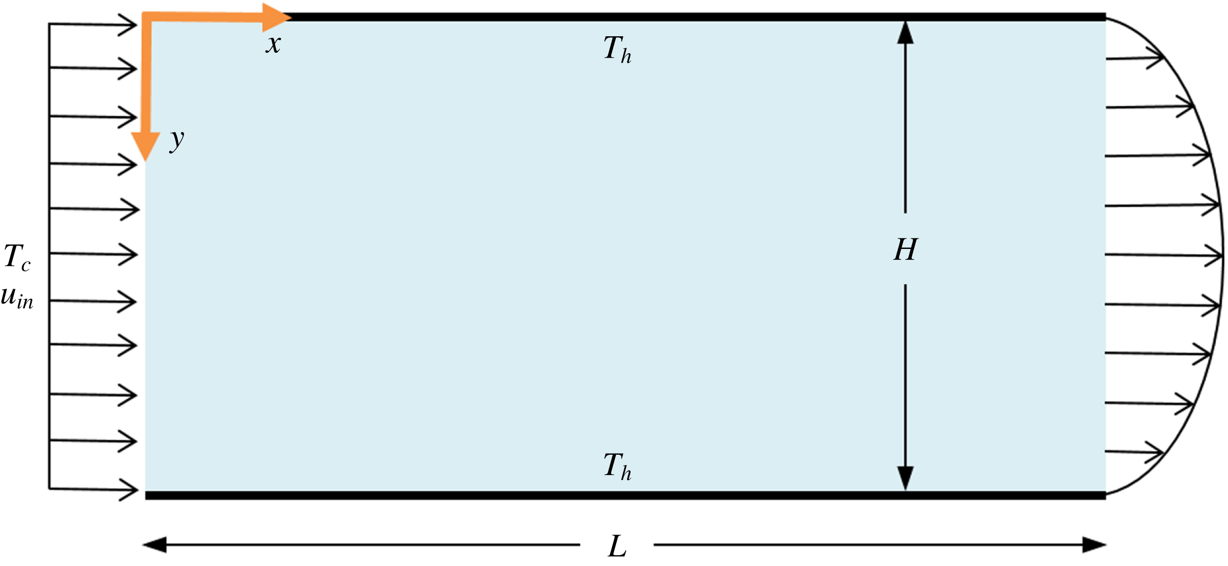
A transient, two-way coupled hybrid Eulerian–Lagrangian model is used to characterize nanofluid flow, heat transfer and particle distribution in a micro/minichannel. The problem selected for this study is related to a channel with a rectangular cross-sectional area (with a height of
 $H$
and width of
 $W$
) and a channel length of
 $L$
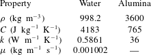
, as shown in figure 1. (All mathematical variable are defined in the Nomenclature at the end of the paper.) In the two-way coupling approach, Lagrangian treatment of the particle phase is combined with Eulerian treatment of the fluid phase, taking into account hydrodynamic and thermal interactions between the two phases. The fluid-phase governing equations are described using a vorticity–stream function formulation, whereas the particle-phase governing equations take into account drag, Brownian motion, thermophoresis, slip-shear-induced lift, gravity and buoyancy body forces, and particle–wall collisions. Alumina nanoparticles dispersed in a water base fluid are used (properties listed in table 1). The following assumptions and conditions are maintained throughout this study.
Schematic representation of the microchannel under investigation.

Physical properties of base fluid and nanoparticles.

(i) The flow is two-dimensional
 $(W\gg H)$
, Newtonian and incompressible.
(ii) The flow Reynolds number
$Re$
is restricted to the laminar regime.(iii) Radiative heat transfer is negligible since the radiation–conduction number
$N_{RC}=\unicode[STIX]{x1D70E}T_{h}^{3}H/k\ll 1$
(Al-Amri & El-Shaarawi Reference Al-Amri and El-Shaarawi2010; Atashafrooz & Nassab Reference Atashafrooz and Nassab2012) for the conditions of this study.
$N_{RC}$
quantifies the importance of surface radiation relative to its conduction counterpart in internal channel flows.(iv) Viscous dissipation and particle rotation are neglected.
(v) All surfaces are impermeable and electrically neutral, with energy dissipation by viscous damping in particle–wall collisions neglected.
(vi) The standard Boussinesq approximation is used to account for fluid density differences in the buoyancy source term, with fluid density assumed constant everywhere else. This is justified because
$\unicode[STIX]{x1D6FD}_{f}\unicode[STIX]{x0394}T_{f,max}=0.0125\ll 1$
, where
$\unicode[STIX]{x1D6FD}_{f}=2.09\times 10^{-4}~\text{K}^{-1}$
.(vii) All nanoparticles are non-deformable, non-reactive, spherical and have the same size.
(viii) The point-mass approximation of the particle phase is utilized (since the size of the particles is considerably smaller than the Eulerian grid) such that particles are treated as volumeless mathematical points with surface-averaged physical models used to describe all interphase fluid–particle exchanges (Migdal & Agosta Reference Migdal and Agosta1967; Durst, Miloievic & Schönung Reference Durst, Miloievic and Schönung1984).
(ix) Collisional, colloidal and hydrodynamic particle–particle interactions are ignored due to the relatively low particle volume fractions under consideration.
(x) It is assumed that nanoparticles are sterically protected against particle clustering effects such as soft agglomeration and hard aggregation (Yu et al. Reference Yu, Chen, Liang, Xu, Lee, Liang, Tao and Deng2017; Mahian et al. Reference Mahian, Kolsi, Amani, Estellé, Ahmadi, Kleinstreuer, Marshall, Siavashi, Taylor and Niazmand2019). Therefore, the nanofluid exhibits Newtonian behaviour (Kim et al. Reference Kim, Kim, Lee and Park2011).






2.1 Continuous-phase governing equations
The carrier fluid phase is described from an Eulerian continuous perspective. The continuum description of the fluid phase is justified based on
 $Kn_{p}=MFP_{f}/D_{p}=0.3~\text{nm}/20~\text{nm}<1$
, in which nanoparticle diameter
 $D_{p}$
is used as a characteristic length, indicating negligible slip-boundary effects at the interface between fluid and particle phases (Michaelides Reference Michaelides2013, Reference Michaelides2014). Utilizing a vorticity–stream function formulation, the fluid governing equations are
 $$\begin{eqnarray}\displaystyle & \displaystyle \frac{\unicode[STIX]{x2202}^{2}\unicode[STIX]{x1D713}_{f}}{\unicode[STIX]{x2202}x^{2}}+\frac{\unicode[STIX]{x2202}^{2}\unicode[STIX]{x1D713}_{f}}{\unicode[STIX]{x2202}y^{2}}=-\unicode[STIX]{x1D714}_{f}, & \displaystyle\end{eqnarray}$$
 $$\begin{eqnarray}\displaystyle & \displaystyle \frac{\unicode[STIX]{x2202}\unicode[STIX]{x1D714}_{f}}{\unicode[STIX]{x2202}t_{f}}+u_{f}\frac{\unicode[STIX]{x2202}\unicode[STIX]{x1D714}_{f}}{\unicode[STIX]{x2202}x}+v_{f}\frac{\unicode[STIX]{x2202}\unicode[STIX]{x1D714}_{f}}{\unicode[STIX]{x2202}y}=\unicode[STIX]{x1D708}_{f}\left(\frac{\unicode[STIX]{x2202}^{2}\unicode[STIX]{x1D714}_{f}}{\unicode[STIX]{x2202}x^{2}}+\frac{\unicode[STIX]{x2202}^{2}\unicode[STIX]{x1D714}_{f}}{\unicode[STIX]{x2202}y^{2}}\right)+g\unicode[STIX]{x1D6FD}_{f}\left(\frac{\unicode[STIX]{x2202}T_{f}}{\unicode[STIX]{x2202}x}\right)+s_{pm}, & \displaystyle\end{eqnarray}$$
 $$\begin{eqnarray}\displaystyle & \displaystyle \frac{\unicode[STIX]{x2202}T_{f}}{\unicode[STIX]{x2202}t_{f}}+u_{f}\frac{\unicode[STIX]{x2202}T_{f}}{\unicode[STIX]{x2202}x}+v_{f}\frac{\unicode[STIX]{x2202}T_{f}}{\unicode[STIX]{x2202}y}=\unicode[STIX]{x1D6FC}_{f}\left(\frac{\unicode[STIX]{x2202}^{2}T_{f}}{\unicode[STIX]{x2202}x^{2}}+\frac{\unicode[STIX]{x2202}^{2}T_{f}}{\unicode[STIX]{x2202}y^{2}}\right)+s_{pe}. & \displaystyle\end{eqnarray}$$
Equation (2.1) is the stream function equation (which identically satisfies continuity), equation (2.2) is the vorticity transport equation and (2.3) is the energy equation. The first term on the left-hand side of (2.2)–(2.3) is the transient term, the second and third terms on the left-hand side of (2.2)–(2.3) represent convection and the first term on the right-hand side of (2.2)–(2.3) represents diffusion. The second term on the right-hand side of (2.2) is the natural convection source term (utilizing the Boussinesq approximation), while the last terms on the right-hand side of (2.2)–(2.3) represent the particle source terms (detailed in § 2.3). The vorticity transport equation (2.2) is derived from the incompressible momentum equation by eliminating pressure as a dependent variable via cross-differentiation. Equations (2.1)–(2.3) are written in non-dimensional form as follows:
 $$\begin{eqnarray}\displaystyle & \displaystyle \frac{\unicode[STIX]{x2202}^{2}\unicode[STIX]{x1D6F9}_{f}}{\unicode[STIX]{x2202}X^{2}}+\frac{\unicode[STIX]{x2202}^{2}\unicode[STIX]{x1D6F9}_{f}}{\unicode[STIX]{x2202}Y^{2}}=-\unicode[STIX]{x1D6FA}_{f}, & \displaystyle\end{eqnarray}$$
 $$\begin{eqnarray}\displaystyle & \displaystyle \frac{\unicode[STIX]{x2202}\unicode[STIX]{x1D6FA}_{f}}{\unicode[STIX]{x2202}\unicode[STIX]{x1D70F}_{f}}+U_{f}\frac{\unicode[STIX]{x2202}\unicode[STIX]{x1D6FA}_{f}}{\unicode[STIX]{x2202}X}+V_{f}\frac{\unicode[STIX]{x2202}\unicode[STIX]{x1D6FA}_{f}}{\unicode[STIX]{x2202}Y}=\frac{1}{Re}\left(\frac{\unicode[STIX]{x2202}^{2}\unicode[STIX]{x1D6FA}_{f}}{\unicode[STIX]{x2202}X^{2}}+\frac{\unicode[STIX]{x2202}^{2}\unicode[STIX]{x1D6FA}_{f}}{\unicode[STIX]{x2202}Y^{2}}\right)+Ri\left(\frac{\unicode[STIX]{x2202}\unicode[STIX]{x1D703}_{f}}{\unicode[STIX]{x2202}X}\right)+S_{pm}, & \displaystyle\end{eqnarray}$$
 $$\begin{eqnarray}\displaystyle & \displaystyle \frac{\unicode[STIX]{x2202}\unicode[STIX]{x1D703}_{f}}{\unicode[STIX]{x2202}\unicode[STIX]{x1D70F}_{f}}+U_{f}\frac{\unicode[STIX]{x2202}\unicode[STIX]{x1D703}_{f}}{\unicode[STIX]{x2202}X}+V_{f}\frac{\unicode[STIX]{x2202}\unicode[STIX]{x1D703}_{f}}{\unicode[STIX]{x2202}Y}=\frac{1}{Re\,Pr}\left(\frac{\unicode[STIX]{x2202}^{2}\unicode[STIX]{x1D703}_{f}}{\unicode[STIX]{x2202}X^{2}}+\frac{\unicode[STIX]{x2202}^{2}\unicode[STIX]{x1D703}_{f}}{\unicode[STIX]{x2202}Y^{2}}\right)+S_{pe}. & \displaystyle\end{eqnarray}$$
Expressions for the source terms on the right-hand side of (2.5)–(2.6) are detailed in § 2.3. The non-dimensional velocities are given as
 $$\begin{eqnarray}U_{f}=\frac{\unicode[STIX]{x2202}\unicode[STIX]{x1D6F9}_{f}}{\unicode[STIX]{x2202}Y},\quad V_{f}=-\frac{\unicode[STIX]{x2202}\unicode[STIX]{x1D6F9}_{f}}{\unicode[STIX]{x2202}X}.\end{eqnarray}$$
It is worth mentioning that the vorticity–stream function formulation has also been used for the study of more complicated two-dimensional (2D) geometries, such as lid-driven flow in a triangular cavity (Ribbens, Watson & Wang Reference Ribbens, Watson and Wang1994; Li & Tang Reference Li and Tang1996; Erturk & Gokcol Reference Erturk and Gokcol2007; Wang & Shi Reference Wang and Shi2014), lid-driven flow in wavy cavities (Öztop et al. Reference Öztop, Sakhrieh, Abu-Nada and Al-Salem2017) and natural convection in triangular enclosures (Akinsete & Coleman Reference Akinsete and Coleman1982; Asan & Namli Reference Asan and Namli2000; Varol, Koca & Oztop Reference Varol, Koca and Oztop2006). Moreover, Jyotsna & Vanka (Reference Jyotsna and Vanka1995) used a multi-grid technique for viscous flow in a triangular cavity. In general, the key challenges that should be addressed in the extension to irregular-shaped geometries are finding the appropriate geometric coordinate transformations, transformation metrics, discretization schemes and vorticity boundary conditions at the corners. For example, for the case of a triangular-shaped lid-driven cavity, the following general steps can be followed to break down the problem.
(1) It is possible to map a general triangle from the physical domain into a right-angled triangle in the computational domain using geometric coordinate transformations.
(2) This is followed by transformation of the governing equations and boundary conditions in a vorticity–stream function formulation for the unknowns
$\unicode[STIX]{x1D6F9}_{f},\unicode[STIX]{x1D6FA}_{f}$
and
$\unicode[STIX]{x1D703}_{f}$
from the physical domain variables into the transformation domain variables using transformation metrics.(3) After that, a finite difference representation of the transformed governing equations and boundary conditions is performed using discretization schemes. Special attention is required here for the vorticity boundary conditions at the corners.
(4) Finally, the solved
$\unicode[STIX]{x1D6F9}_{f},\unicode[STIX]{x1D6FA}_{f}$
and
$\unicode[STIX]{x1D703}_{f}$
fields are transformed back from the computational domain to the physical domain.


2.2 Continuous-phase boundary conditions
The non-dimensional boundary conditions for the Eulerian fluid phase are given as follows:
 $$\begin{eqnarray}\displaystyle & \displaystyle 0<X<1,\quad Y=0:\quad \unicode[STIX]{x1D6F9}_{f}=0,\quad \unicode[STIX]{x1D6FA}_{f}=-\frac{\unicode[STIX]{x2202}^{2}\unicode[STIX]{x1D6F9}_{f}}{\unicode[STIX]{x2202}Y^{2}},\quad \unicode[STIX]{x1D703}_{f}=1, & \displaystyle\end{eqnarray}$$
 $$\begin{eqnarray}\displaystyle & \displaystyle 0<X<1,\quad Y=1:\quad \unicode[STIX]{x1D6F9}_{f}=\unicode[STIX]{x1D703}_{f}=1,\quad \unicode[STIX]{x1D6FA}_{f}=-\frac{\unicode[STIX]{x2202}^{2}\unicode[STIX]{x1D6F9}_{f}}{\unicode[STIX]{x2202}Y^{2}}, & \displaystyle\end{eqnarray}$$
 $$\begin{eqnarray}\displaystyle & \displaystyle X=0,\quad 0<Y<1:\quad \unicode[STIX]{x1D6F9}_{f}=Y,\quad \unicode[STIX]{x1D6FA}_{f}=-\frac{\unicode[STIX]{x2202}^{2}\unicode[STIX]{x1D6F9}_{f}}{\unicode[STIX]{x2202}X^{2}},\quad \unicode[STIX]{x1D703}_{f}=0, & \displaystyle\end{eqnarray}$$
 $$\begin{eqnarray}\displaystyle & \displaystyle X=1,\quad 0<Y<1:\quad \frac{\unicode[STIX]{x2202}\unicode[STIX]{x1D6F9}_{f}}{\unicode[STIX]{x2202}X}=\frac{\unicode[STIX]{x2202}\unicode[STIX]{x1D6FA}_{f}}{\unicode[STIX]{x2202}X}=\frac{\unicode[STIX]{x2202}\unicode[STIX]{x1D703}_{f}}{\unicode[STIX]{x2202}X}=0. & \displaystyle\end{eqnarray}$$
Thus, the channel upper and lower surfaces are maintained at
 $T_{h}$
with no-slip boundary conditions between the fluid and walls, the flow enters as plug flow at
 $T_{c}$
and zero-gradient conditions in the flow direction are used at the outlet. The no-slip boundary condition at the interface between the fluid and microchannel walls is justified based on
 $Kn_{ch}=MFP_{f}/H=0.3~\text{nm}/50~\unicode[STIX]{x03BC}\text{m}\ll 1$
, in which channel height
 $H$
is used as a characteristic length, indicating negligible slip-boundary effects at the fluid–channel interface. Nonetheless, it is important to note that other parameters can also affect the degree of slip at the fluid–channel interface, such as strength of the solid–fluid coupling, fluid temperature and density of the solid wall, which can be accounted for by appropriately modifying the no-slip boundary condition (Zhang et al.
Reference Zhang, Zhang, Zheng and Ye2010; Zhang, Zhang & Ye Reference Zhang, Zhang and Ye2012).
2.3 Discrete-phase governing equations
The dispersed particle phase is described from a Lagrangian discrete perspective, where properties of a number of computational particles are tracked in time. Each computational particle (also known as a parcel) is a representation of a bundle of many real nanoparticles with identical properties (e.g. size, velocity, temperature). Representing the large number of nanoparticles in a particulate flow using computational particles results in a computationally manageable number of particle equations to be solved. The source terms on the right-hand side of (2.2)–(2.3) and (2.5)–(2.6) represent the particle momentum and energy exchange with the fluid (i.e. the two-way coupling terms), respectively. Two-way coupling entails particles exchanging mass, momentum and energy with the fluid phase. This coupling approach is known as the particle source-in-cell (PSI-cell) method (Crowe, Sharma & Stock Reference Crowe, Sharma and Stock1977). In the PSI-cell coupling method, particle momentum and thermal feedback source terms are introduced into the continuous-phase equations in order to represent momentum and thermal interphase interactions between fluid and particle. The expressions for
 $S_{pm}$
and
 $S_{pe}$
in a single computational cell are defined by tracking (from a Lagrangian perspective) changes in momentum and energy along each computational particle trajectory within the computational cell by the effect of the fluid phase, as follows:
 $$\begin{eqnarray}\displaystyle & \displaystyle S_{pm}=\frac{\unicode[STIX]{x03C0}D_{p}^{3}\,f_{p}}{6\forall _{cell}\,f_{\unicode[STIX]{x1D70C}}}\left(\frac{\unicode[STIX]{x2202}}{\unicode[STIX]{x2202}X}\mathop{\sum }_{j=1}^{N_{cp,cell}}\left(\frac{\text{d}V_{p,j}}{\text{d}\unicode[STIX]{x1D70F}_{f}}-B_{y,j}\right)-\frac{\unicode[STIX]{x2202}}{\unicode[STIX]{x2202}Y}\mathop{\sum }_{j=1}^{N_{cp,cell}}\left(\frac{\text{d}U_{p,j}}{\text{d}\unicode[STIX]{x1D70F}_{f}}-B_{x,j}\right)\right), & \displaystyle\end{eqnarray}$$
 $$\begin{eqnarray}\displaystyle & \displaystyle S_{pe}=\frac{\unicode[STIX]{x03C0}D_{p}^{3}\,f_{p}}{6\forall _{cell}\,f_{\unicode[STIX]{x1D70C}}\,f_{C}}\mathop{\sum }_{j=1}^{N_{cp,cell}}\left(\frac{\text{d}\unicode[STIX]{x1D703}_{p,j}}{\text{d}\unicode[STIX]{x1D70F}_{f}}\right), & \displaystyle\end{eqnarray}$$
where
 $B_{x}$
and
 $B_{y}$
are the non-dimensional sums of all external body forces acting on a particle (i.e. due to gravity and buoyancy forces in this study). A computational cell is centred around each Eulerian grid node, where
 $N_{cp,cell}$
is the number of computational particles within the domain of a computational cell (set to ten times the total number of computational cells in this study). Computational particles are seeded within the computational domain to recover the volume fraction of nanoparticles. Hence, each computational particle is given a statistical weight (i.e. the number of real particles represented by the computational particle) defined by the parcel factor
 $f_{p}$
:
 $$\begin{eqnarray}f_{p}=\frac{N_{p,tot}}{N_{cp,tot}}=\frac{6\unicode[STIX]{x1D719}_{p}\forall _{tot}}{\unicode[STIX]{x03C0}D_{p}^{3}N_{cp,tot}},\end{eqnarray}$$
where
 $N_{p,tot}$
and
 $N_{cp,tot}$
are the total numbers of real nanoparticles and computational particles, respectively. All computational particles have the same
 $f_{p}$
, such that
 $\sum _{j=1}^{N_{cp,tot}}f_{p,j}=N_{p,tot}$
. Equations (2.12)–(2.13) show that the magnitude of the particle source terms is strongly affected by the density ratio
 $f_{\unicode[STIX]{x1D70C}}$
and specific heat capacity ratio
 $f_{C}$
. Moreover, equation (2.14) indicates that when
 $\unicode[STIX]{x1D719}_{p}$
is increased for the same
 $D_{p}$
, the number of real nanoparticles represented by each computational particle increases by means of
 $f_{\unicode[STIX]{x1D70C}}$
.
The dispersed particle-phase dynamics is dominated by particle–fluid interactions. Thus, in the particle motion equations, we consider the effects of drag (Maxey & Riley Reference Maxey and Riley1983), Brownian motion (Abuzeid, Busnaina & Ahmadi Reference Abuzeid, Busnaina and Ahmadi1991), thermophoresis (McNab & Meisen Reference McNab and Meisen1973), transverse slip-shear-induced lift (Saffman Reference Saffman1965), and gravity and buoyancy body forces. As such, Lagrangian tracking of the computational particles is governed by the following equations:
 $$\begin{eqnarray}\frac{\text{d}u_{p}}{\text{d}t_{p}}=\left[\frac{18\unicode[STIX]{x1D707}_{f}C_{i}}{\unicode[STIX]{x1D70C}_{p}D_{p}^{2}C_{c}}(u_{f}-u_{p})\right]+\left[\frac{\unicode[STIX]{x1D6FF}}{m_{p}}\sqrt{\frac{6\unicode[STIX]{x03C0}\unicode[STIX]{x1D705}_{B}T_{f}D_{p}\unicode[STIX]{x1D707}_{f}}{C_{c}\unicode[STIX]{x0394}t_{p}}}\right]+\left[\frac{u_{T}}{\unicode[STIX]{x1D70F}_{m}}\right],\end{eqnarray}$$
 $$\begin{eqnarray}\displaystyle \frac{\text{d}v_{p}}{\text{d}t_{p}} & = & \displaystyle \left[\frac{18\unicode[STIX]{x1D707}_{f}C_{i}}{\unicode[STIX]{x1D70C}_{p}D_{p}^{2}C_{c}}(v_{f}-v_{p})\right]+\left[\frac{\unicode[STIX]{x1D6FF}}{m_{p}}\sqrt{\frac{6\unicode[STIX]{x03C0}\unicode[STIX]{x1D705}_{B}T_{f}D_{p}\unicode[STIX]{x1D707}_{f}}{C_{c}\unicode[STIX]{x0394}t_{p}}}\right]+\left[\frac{v_{T}}{\unicode[STIX]{x1D70F}_{m}}\right]+\left[g\left(1-\frac{\unicode[STIX]{x1D70C}_{f}}{\unicode[STIX]{x1D70C}_{p}}\right)\right]\nonumber\\ \displaystyle & & \displaystyle +\left[\frac{9.69}{\unicode[STIX]{x03C0}\unicode[STIX]{x1D70C}_{p}D_{p}}\sqrt{\unicode[STIX]{x1D70C}_{f}\unicode[STIX]{x1D707}_{f}\left|\frac{\unicode[STIX]{x2202}u_{f}}{\unicode[STIX]{x2202}y}\right|}(u_{f}-u_{p})\text{sgn}\left(\frac{\unicode[STIX]{x2202}u_{f}}{\unicode[STIX]{x2202}y}\right)\right],\end{eqnarray}$$
 $$\begin{eqnarray}\frac{\text{d}x_{p}}{\text{d}t_{p}}=u_{p},\quad \frac{\text{d}y_{p}}{\text{d}t_{p}}=v_{p}.\end{eqnarray}$$
The first three terms on the right-hand side of (2.15)–(2.16) represent steady-state drag force due to relative motion between fluid and particle phases, amplitude of Brownian force over a time interval
 $\unicode[STIX]{x0394}t_{p}$
due to random fluid molecule collisions with the particle phase and thermophoretic force due to temperature gradient in the fluid phase, respectively. The fourth term on the right-hand side of (2.16) represents gravity and buoyancy (hydrostatic pressure gradient) forces. The last term on the right-hand side of (2.16) represents the transverse slip-shear-induced lift (Saffman lift) force for small
 $Re_{p}$
values, which acts in the direction of the highest slip velocity magnitude.
In our modelling approach, the random motion of nanoparticles is taken to be a result of a continuous random force acting on the nanoparticles. Thus, in (2.15)–(2.16), Brownian force is expressed as a white-noise stochastic process. On the other hand, thermophoretic force is expressed as the ratio between thermophoretic velocity and particle momentum relaxation time. The thermophoretic velocity is expressed as
 $$\begin{eqnarray}u_{T}=\frac{-K_{T}\unicode[STIX]{x1D707}_{f}}{\unicode[STIX]{x1D70C}_{f}T_{f}}\frac{\text{d}T_{f}}{\text{d}x},\quad v_{T}=\frac{-K_{T}\unicode[STIX]{x1D707}_{f}}{\unicode[STIX]{x1D70C}_{f}T_{f}}\frac{\text{d}T_{f}}{\text{d}y}.\end{eqnarray}$$
The particle momentum relaxation time
 $\unicode[STIX]{x1D70F}_{m}$
is the characteristic timescale for the particles, defined as
 $$\begin{eqnarray}\unicode[STIX]{x1D70F}_{m}=\frac{\unicode[STIX]{x1D70C}_{p}D_{p}^{2}C_{c}}{18\unicode[STIX]{x1D707}_{f}};\end{eqnarray}$$
 $\unicode[STIX]{x1D70F}_{m}$
measures the time required for a particle to respond to changes in the carrier fluid velocity. Other hydrodynamic forces, such as Basset history, virtual mass (added mass), inertial pressure gradient, Faxen and slip-rotation-induced lift (Magnus lift) have been reported to have a small effect for nano-sized particles with small
 $Re_{p}$
values and are not considered in the present formulation.
Using non-dimensional quantities listed in the Nomenclature, the non-dimensional form of (2.15)–(2.17) is expressed as follows:
 $$\begin{eqnarray}\frac{\text{d}U_{p}}{\text{d}\unicode[STIX]{x1D70F}_{p}}=\left[\frac{C_{i}}{St}(U_{f}-U_{p})\right]+\left[\frac{\unicode[STIX]{x1D6FF}}{St}\sqrt{\frac{2}{Pe_{B}\unicode[STIX]{x0394}\unicode[STIX]{x1D70F}_{p}}}\right]+\left[\frac{1}{St\,Pe_{T}}\left(\frac{\unicode[STIX]{x2202}\unicode[STIX]{x1D703}_{f}}{\unicode[STIX]{x2202}X}\right)\right],\end{eqnarray}$$
 $$\begin{eqnarray}\displaystyle \frac{\text{d}V_{p}}{\text{d}\unicode[STIX]{x1D70F}_{p}} & = & \displaystyle \left[\frac{C_{i}}{St}(V_{f}-V_{p})\right]+\left[\frac{\unicode[STIX]{x1D6FF}}{St}\sqrt{\frac{2}{Pe_{B}\unicode[STIX]{x0394}\unicode[STIX]{x1D70F}_{p}}}\right]+\left[\frac{1}{St\,Pe_{T}}\left(\frac{\unicode[STIX]{x2202}\unicode[STIX]{x1D703}_{f}}{\unicode[STIX]{x2202}Y}\right)\right]+\left[\frac{1}{Fr^{2}}(1-f_{\unicode[STIX]{x1D70C}})\right]\nonumber\\ \displaystyle & & \displaystyle +\left[\frac{9.69}{\unicode[STIX]{x03C0}}\sqrt{\frac{C_{c}\,f_{\unicode[STIX]{x1D70C}}}{18\,St}\left|\frac{\unicode[STIX]{x2202}U_{f}}{\unicode[STIX]{x2202}Y}\right|}(U_{f}-U_{p})\text{sgn}\left(\frac{\unicode[STIX]{x2202}U_{f}}{\unicode[STIX]{x2202}Y}\right)\right],\end{eqnarray}$$
 $$\begin{eqnarray}\frac{\text{d}X_{p}}{\text{d}\unicode[STIX]{x1D70F}_{p}}=U_{p},\quad \frac{\text{d}Y_{p}}{\text{d}\unicode[STIX]{x1D70F}_{p}}=V_{p}.\end{eqnarray}$$
It can be seen from (2.20) to (2.21) that Stokes number
 $St$
and density ratio
 $f_{\unicode[STIX]{x1D70C}}$
are key dimensionless parameters affecting contributions from the different particle force terms.
In order to account for fluid inertia effects (i.e. whenever the
 $Re_{p}\ll 1$
condition is not satisfactorily met), Stokes drag is corrected by a fluid inertia correction factor, given using the empirical correlation of Schiller & Naumann (Reference Schiller and Naumann1933) as follows:
 $$\begin{eqnarray}C_{i}=1+0.15Re_{p}^{0.687}.\end{eqnarray}$$
This correlation is valid up to
 $Re_{p}<800$
. Due to their very small size, nanoparticles typically have
 $Re_{p}$
values
 $\ll 1$
(Mahian et al.
Reference Mahian, Kolsi, Amani, Estellé, Ahmadi, Kleinstreuer, Marshall, Siavashi, Taylor and Niazmand2019). Therefore, nanofluid flow is within the validity range of the Schiller and Naumann correlation, where higher values of
 $Re_{p}$
are not expected to occur and
 $C_{i}\approx 1$
. This means that the fluid flow seen by nanoparticles remains laminar and principally within the Stokes regime, where viscous effects are dominant and no flow separation around the particles occurs. Similarly, for nano-sized particles, Stokes drag is corrected by a Cunningham slip correction factor to account for any slip-boundary effects at the particle–fluid interface that result in a drop in the drag force, given as (Davies Reference Davies1945)
 $$\begin{eqnarray}C_{c}=1+2Kn_{p}\left(1.257+0.4\exp \left(\frac{-1.1}{2Kn_{p}}\right)\right).\end{eqnarray}$$
This correlation is valid for
 $Re_{p}<0.25$
and submicron particles in Stokesian flow conditions (i.e.
 $Kn_{p}\ll 1$
). Although the empirical correlation in (2.24) has been devised for systems with a gaseous fluid phase, it is reasonable to assume that the experimental data of the Stokesian drag for particles in air would agree with the corresponding drag on small, solid nanoparticles in liquids, for the same values of
 $Re_{p}$
and
 $Kn_{p}$
(Michaelides Reference Michaelides2014, Reference Michaelides2015). Since the validity conditions for (2.24) are maintained in this study, and due to the lack of an equivalent correlation specifically designed for nanofluid flow, we extend its applicability to nanoparticles dispersed in liquids. Ultimately, since
 $Kn_{p}\ll 1$
for nano-sized particles in liquids, slip-boundary effects will be quite small and
 $C_{c}\approx 1$
. In (2.20)–(2.21), Stokes number
 $St$
is a measure of the particle inertia. When
 $St\ll 1$
, particles will closely follow the fluid, whereas for
 $St>1$
, the fluid and particles will have a relatively large relative velocity. As a characteristic timescale for the fluid, the fluid laminar convection time
 $\unicode[STIX]{x1D70F}_{F}$
is defined as
 $$\begin{eqnarray}\unicode[STIX]{x1D70F}_{F}=\frac{H}{u_{in}}.\end{eqnarray}$$
For evaluation of the Brownian and thermophoretic forces, the Brownian Péclet number
 $Pe_{B}$
and thermophoretic Péclet number
 $Pe_{T}$
represent the relative importance of convective forces compared to Brownian diffusive forces and thermophoretic diffusive forces, respectively. The corrected Brownian diffusivity
 $D_{B}$
is defined as
 $$\begin{eqnarray}D_{B}=\frac{\unicode[STIX]{x1D705}_{B}T_{f}C_{c}}{3\unicode[STIX]{x03C0}D_{p}\unicode[STIX]{x1D707}_{f}},\end{eqnarray}$$
while we define the thermophoretic diffusivity
 $D_{T}$
as
 $$\begin{eqnarray}D_{T}=-K_{T}\frac{\unicode[STIX]{x1D707}_{f}(T_{h}-T_{c})}{\unicode[STIX]{x1D70C}_{f}T_{f}}.\end{eqnarray}$$
McNab & Meisen (Reference McNab and Meisen1973) derived
 $K_{T}$
for liquids from experimental data, as follows:
 $$\begin{eqnarray}K_{T}=0.26\frac{k_{f}}{2k_{f}+k_{p}}.\end{eqnarray}$$
It is assumed that there are no spatial temperature variations within the body of a nanoparticle. This is based on
 $Bi\ll 1$
for metallic nano-sized particles. Thus, particle temperature is tracked by applying the first law of thermodynamics on the particle:
 $$\begin{eqnarray}m_{p}C_{p}\frac{\text{d}T_{p}}{\text{d}t_{p}}=\unicode[STIX]{x03C0}hD_{p}^{2}(T_{f}-T_{p}).\end{eqnarray}$$
In non-dimensional form, equation (2.29) is expressed as
 $$\begin{eqnarray}\frac{\text{d}\unicode[STIX]{x1D703}_{p}}{\text{d}\unicode[STIX]{x1D70F}_{p}}=\frac{St_{\unicode[STIX]{x1D703}}Nu_{p}}{2}(\unicode[STIX]{x1D703}_{f}-\unicode[STIX]{x1D703}_{p}).\end{eqnarray}$$
Thermal Stokes number
 $St_{\unicode[STIX]{x1D703}}$
, defined in terms of
 $\unicode[STIX]{x1D70F}_{\unicode[STIX]{x1D703}}$
, is a measure of the thermal response of a particle. The particle thermal relaxation time
 $\unicode[STIX]{x1D70F}_{\unicode[STIX]{x1D703}}$
, which measures the time required for the particle to respond to changes in the carrier fluid temperature, is defined as (Michaelides Reference Michaelides2013)
 $$\begin{eqnarray}\unicode[STIX]{x1D70F}_{\unicode[STIX]{x1D703}}=\frac{C_{p}\unicode[STIX]{x1D70C}_{p}D_{p}^{2}}{12k_{f}}.\end{eqnarray}$$
Ranz & Marshall (Reference Ranz and Marshall1952) obtained an empirical correlation for the convective heat transfer of small solid particles, as follows:
 $$\begin{eqnarray}Nu_{p}=2+0.6Pr^{1/3}Re_{p}^{1/2}.\end{eqnarray}$$
This correlation should only be used for solid spheres in the absence of mass transfer on the particle surface and is valid up to
 $Re_{p}<1\times 10^{4}$
(Michaelides, Crowe & Schwarzkopf Reference Michaelides, Crowe and Schwarzkopf2017), which is applicable to the range of
 $Re_{p}$
in the current study and in typical nanofluid systems where
 $Re_{p}\ll 1$
. Moreover, the Ranz & Marshall correlation exhibits the correct asymptotic behaviour for steady-state heat transfer from a sphere as
 $Re_{p}\rightarrow 0$
where
 $Nu_{p}=2$
. Since
 $Re_{p}$
for nanoparticles is indeed
 $\ll 1$
, conduction is the dominant mode of heat transfer from nanoparticles to the surrounding fluid, and
 $Nu_{p}\approx 2$
according to (2.32). Therefore, due to the lack of an equivalent correlation specifically designed for nanofluid flow, the Ranz & Marshall correlation has been extensively adopted in the nanofluid literature for the description of convective heat transfer between solid nanoparticles and the surrounding fluid.
The point treatment of surface forces and heat transfer, rather than a surface-resolved treatment, allows us to avoid the tremendous computational effort necessary for resolving the fluid flow and temperature fields around each particle in practical particulate flow systems. Thus, although particle volume is not explicitly resolved in the Eulerian–Lagrangian approach based on the point-mass approximation, particle volume has a great effect on most of the closure models used to describe the interphase fluid–particle exchanges. This effect can be clearly observed from the strong dependence of such dimensionless parameters as
 $St$
,
 $St_{\unicode[STIX]{x1D703}}$
,
 $Re_{p}$
,
 $Pe_{B}$
,
 $Nu_{p}$
,
 $f_{p}$
,
 $K_{n,p}$
,
 $C_{c}$
and
 $Bi$
on particle diameter
 $D_{p}$
.
2.4 Discrete-phase boundary conditions
Initially, nanoparticles are randomly distributed within the base fluid in the channel with
 $U_{p}=V_{p}=\unicode[STIX]{x1D703}_{p}=0$
(i.e. both phases are initially at rest within the channel). A nanoparticle that reaches the channel outlet is reinjected at the channel inlet at a randomized
 $y$
-location with
 $X_{p}=V_{p}=\unicode[STIX]{x1D703}_{p}=0$
and
 $U_{p}=1$
.
Regarding particle–wall interactions, a particle may adhere to the wall or rebound from it upon a collision, depending on the particle kinetic energy and particle–wall interaction potential. The particle rebounds when its kinetic energy is sufficient to escape adhesive forces at the wall surface. We define a collision to take place whenever the distance between particle surface and wall surface is smaller than or equal to a particle–wall equilibrium separation distance
 $\unicode[STIX]{x1D709}$
, where
 $\unicode[STIX]{x1D709}$
mimics asperities at the interacting surfaces. By taking the particle–wall van der Waals interaction potential
 $E$
to be unchanged before and after collision, we can link the particle energy before and after collision with a wall using the normal coefficient of restitution
 $r$
, as follows (Friedlander Reference Friedlander1977):
 $$\begin{eqnarray}\frac{m_{p}v_{p,re}^{2}}{2}+E=\left(\frac{m_{p}v_{p,i}^{2}}{2}+E\right)r^{2},\end{eqnarray}$$
where
 $r=1$
for a perfectly elastic collision and
 $r<1$
due to dissipative processes. Physically, the parameter
 $r$
is a function of wall and nanoparticle material, size, shape, surface roughness, wetness, collision velocity, etc. Although there are many works that have attempted to determine the value of
 $r$
for microparticles in gas–solid systems (Hu et al.
Reference Hu, Luo, Wang, Junjie and Fan2019), no such works have been reported for the case of nanoparticle dispersions in liquid media. Therefore,
 $r$
is treated as a free parameter in this study. We assume that particle deposition does not alter the roughness of channel walls beyond the original surface asperities. In reality, nanoparticle deposition, especially at high particle loadings, can increase the surface roughness of channel walls, which can affect the degree of boundary slip at the walls and even the overall volumetric flow rate of the nanofluid (Zhang et al.
Reference Zhang, Yuan, Liu, Cheng, Ye and Ding2018). Using (2.33), we can define a critical capture normal velocity
 $v_{C}$
at which
 $v_{p,re}=0$
, as follows:
 $$\begin{eqnarray}v_{C}=\sqrt{\frac{12E}{\unicode[STIX]{x03C0}\unicode[STIX]{x1D70C}_{p}D_{p}^{3}}\left(\frac{1-r^{2}}{r^{2}}\right)}.\end{eqnarray}$$
Thus, if
 $|v_{p,i}|\leqslant v_{C}$
, the particle cannot escape the wall adhesive forces and, thus, it sticks to the wall (i.e. particle deposition) without rolling or sliding. On the other hand, if
 $|v_{p,i}|>v_{C}$
, the particle rebounds from the wall (i.e. particle reflection) with a particle rebound normal velocity magnitude as per (2.33). On the other hand, the particle kinetic energy due to motion parallel to the wall is taken to be conserved throughout a collision with the normal component of velocity
 $v_{p,i}$
independent of tangential motion. In (2.33)–(2.34),
 $E$
is given from (Dahneke Reference Dahneke1971):
 $$\begin{eqnarray}E=\left|\frac{-A_{H}D_{p}}{12\unicode[STIX]{x1D709}}\right|,\end{eqnarray}$$
where
 $A_{H}$
for alumina nanoparticles in a water base fluid interacting with an alumina wall is
 $2.75\times 10^{-20}$
J (Ackler, French & Chiang Reference Ackler, French and Chiang1996) and
 $\unicode[STIX]{x1D709}$
is set to 4 Å. The approximate expression in (2.35) is valid as long as the ratio
 $\unicode[STIX]{x1D709}/D_{p}\ll 1$
(Gregory Reference Gregory1981), which applies to all
 $D_{p}$
values in this study.
3 Computational algorithm and coupling approach
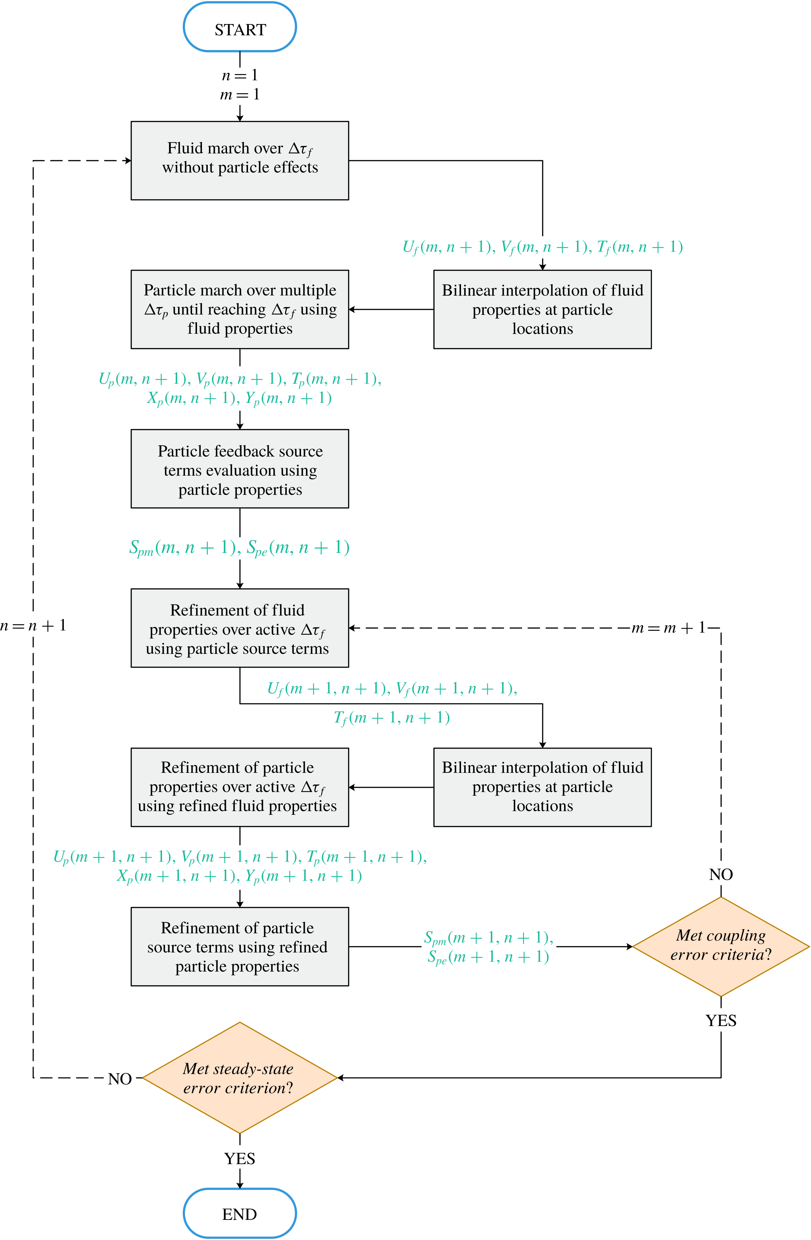
In this study, the Eulerian and Lagrangian fields are solved using a hybrid transient coupling approach implemented via an in-house code developed in the MATLAB environment. In this approach, coupling between the two phases is done in an iterative manner, where during a single fluid (Eulerian) time step, the particle phase is tracked over multiple particle (Lagrangian) time steps. This approach is used in order to avoid the high computational cost associated with equating the fluid and particle time steps (since
 $\unicode[STIX]{x0394}t_{p}\ll \unicode[STIX]{x0394}t_{f}$
). The coupling and marching procedures in the current approach are detailed as follows.
(1) Using the finite difference method, the fluid phase is marched in time for a single fluid (Eulerian) time step ((2.4)–(2.6)) without account for particle contributions.
(2) Using the Euler implicit method, the particle phase is tracked over multiple particle (Lagrangian) time steps ((2.20)–(2.22) and (2.30)), where fluid properties at cell boundaries are assumed constant as seen by the particles. Particles are tracked until reaching the end of the fluid (Eulerian) time step.
(3) Using the required particle-phase properties (
$U_{p},V_{p},\unicode[STIX]{x1D703}_{p}$
) at the end of the fluid (Eulerian) time step, particle momentum and energy source terms ((2.12)–(2.13)) are evaluated.(4) The fluid-phase equations are recalculated for the current fluid (Eulerian) time step, but with addition of the particle source terms.
(5) The particle-phase equations are recalculated during the current fluid (Eulerian) time step over multiple particle (Lagrangian) time steps using the updated fluid-phase properties.
(6) The particle source terms are recalculated using the updated particle-phase properties at the end of the current fluid (Eulerian) time step.
(7) The differences in fluid and particle properties before and after updating the particle source terms are quantified using coupling residual errors, defined as follows:
where(3.1a )$$\begin{eqnarray}\displaystyle & \displaystyle \max _{1\leqslant i\leqslant N_{\mathit{cp}}}|u_{p}^{m+1}-u_{p}^{m}|_{i}\leqslant 10^{-7}, & \displaystyle\end{eqnarray}$$
(3.1b )$$\begin{eqnarray}\displaystyle & \displaystyle \max _{\substack{ 1\leqslant i\leqslant N_{x} \\ 1\leqslant j\leqslant N_{y}}}|u_{f}^{m+1}-u_{f}^{m}|_{i,j}\leqslant 10^{-7}, & \displaystyle\end{eqnarray}$$
$m$
denotes the coupling refinement iteration number. Steps (4)–(6) are repeated for the current fluid (Eulerian) time step until the fluid and particle coupling residual errors stopping criteria are met.(8) Upon satisfying the coupling residual errors stopping criteria, the fluid phase is marched in time into the next fluid (Eulerian) time step and steps (1)–(7) are repeated.
(9) Steps (1)–(8) are repeated until a steady-state residual error stopping criterion is met. The steady-state residual error is calculated by comparing the maximum difference in fluid temperature across the domain for two successive time steps, as follows:
(3.2)where$$\begin{eqnarray}\max _{\substack{ 1\leqslant i\leqslant N_{x} \\ 1\leqslant j\leqslant N_{y}}}|\unicode[STIX]{x1D703}_{f}^{n+1}-\unicode[STIX]{x1D703}_{f}^{n}|_{i,j}\leqslant 10^{-7},\end{eqnarray}$$
$n$
denotes the fluid (Eulerian) time step number.


The described computational algorithm and coupling approach are visually illustrated in the simplified flowchart in figure 2. Solution of the particle governing equations (i.e. (2.20)–(2.22) and (2.30)) requires computation of forces exerted by the fluid on particles, as detailed in § 2.3 (i.e. drag, Brownian, thermophoretic and slip-shear lift forces). Since particle governing equations are solved using an implicit technique, evaluation of these fluid–particle forces requires knowledge of fluid properties (e.g. velocity and temperature) at the active Eulerian time step (
 $n+1$
). As seen from the flowchart in figure 2, all fluid properties are initially evaluated at
 $n+1$
without accounting for particle contributions (i.e. undisturbed fluid-phase properties). After that, the initial calculation of particle properties takes place, where all fluid–particle forces are computed using the initial estimates of undisturbed fluid properties at
 $n+1$
. Following these initial fluid and particle properties calculations, iterative refinements of fluid and particle properties and particle source terms take place until meeting the coupling residual error stopping criteria described above. Therefore, disturbed fluid properties (i.e. fluid properties with account of particle effects) at particle locations are iteratively refined
 $m$
times during a single Eulerian time step.
Simplified flowchart of the computational algorithm and coupling approach.

All required fluid-phase properties (
 $U_{f},V_{f},\unicode[STIX]{x1D703}_{f}$
) are obtained at the location of a particle using bilinear interpolation of fluid properties at boundaries of the computational cell encompassing the particle. Furthermore, it is important to note that during an active Eulerian time step, the zero-mean, unit-variance independent Gaussian random numbers
 $\unicode[STIX]{x1D6FF}$
used in the nanoparticle Brownian motion calculations need to be different for each Lagrangian time step, but the same during the coupling iterations (steps (1)–(7)) within a single active Eulerian time step. All required random numbers in this study have been generated using the MATLAB built-in Mersenne Twister algorithm, with seeding based on the clock time.
The choice of the particle integration time step
 $\unicode[STIX]{x0394}t_{p}$
for solving the particle governing equations of micro-sized particles should generally be a fraction of the particle relaxation time (Li & Ahmadi Reference Li and Ahmadi1992). However, we find that the hydrodynamic and heat transfer characteristics of the particulate and fluid phases are independent of the choice of
 $\unicode[STIX]{x0394}t_{p}$
for the case of nano-sized particle colloidal dispersions in a laminar liquid flow, provided that the simulations run until reaching steady-state conditions. This is attributed to the very small inertia of nano-sized particles. Thus, the very high computational cost associated with abiding by the above-mentioned
 $\unicode[STIX]{x0394}t_{p}$
condition is deemed unnecessary for nanoparticle colloidal dispersions. Nonetheless, the choice of
 $\unicode[STIX]{x0394}t_{p}$
should be small enough that a computational particle travels a distance much smaller than the Eulerian-phase spatial step size in a single particle time step. This conclusion regarding the choice of
 $\unicode[STIX]{x0394}t_{p}$
is revisited and further reinforced in § 4.
4 Model verification
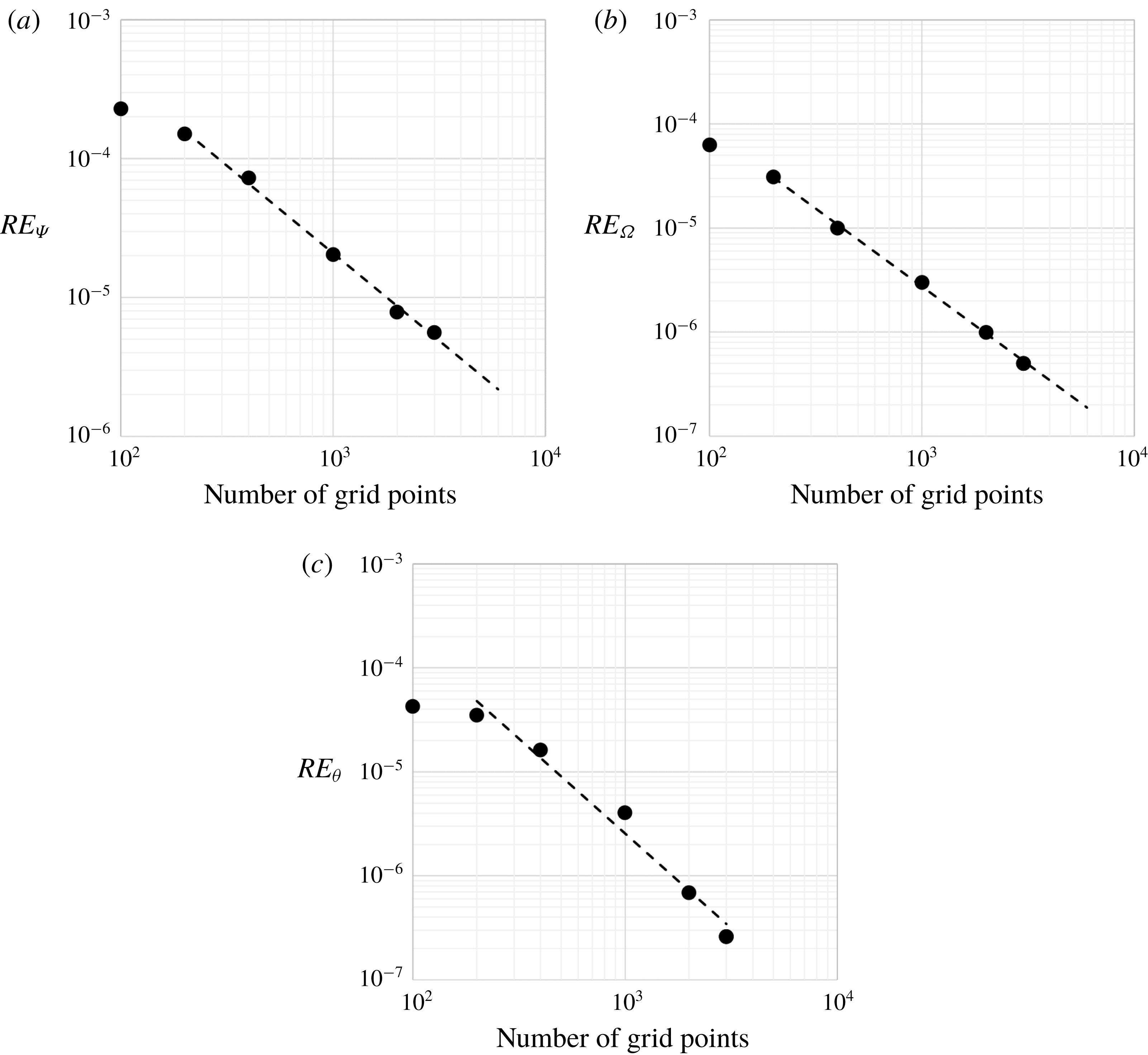
In order to show the error convergence behavior, a formal grid convergence study is performed and the relative errors in three dependent variables,
 $\unicode[STIX]{x1D6F9}_{f}$
,
 $\unicode[STIX]{x1D6FA}_{f}$
and
 $\unicode[STIX]{x1D703}_{f}$
, at the middle of the channel are presented in figure 3. The ‘exact’ solutions,
 $\unicode[STIX]{x1D6F9}_{f,ex}$
,
 $\unicode[STIX]{x1D6FA}_{f,ex}$
and
 $\unicode[STIX]{x1D703}_{f,ex}$
, are approximated to be equal to those of the finest grid (taken at 4000 grid points). The relative error is calculated using the following relation:
 $$\begin{eqnarray}RE_{Z}=\frac{|Z_{f,ex}-Z_{f}|}{Z_{f,ex}},\end{eqnarray}$$
where
 $Z$
denotes
 $\unicode[STIX]{x1D6F9}$
,
 $\unicode[STIX]{x1D6FA}$
or
 $\unicode[STIX]{x1D703}$
. Using a least-square fit of the data points, the relative errors in
 $\unicode[STIX]{x1D6F9}_{f}$
,
 $\unicode[STIX]{x1D6FA}_{f}$
and
 $\unicode[STIX]{x1D703}_{f}$
are converging towards the exact solution at rates of
 $\cong$
1.26, 1.50 and 1.82, respectively, which are consistent with the theoretical order-of-convergence of the employed finite difference discretization.
Grid convergence behaviour in terms of (a)
 $\unicode[STIX]{x1D6F9}_{f}$
, (b)
 $\unicode[STIX]{x1D6FA}_{f}$
and (c)
 $\unicode[STIX]{x1D703}_{f}$
.

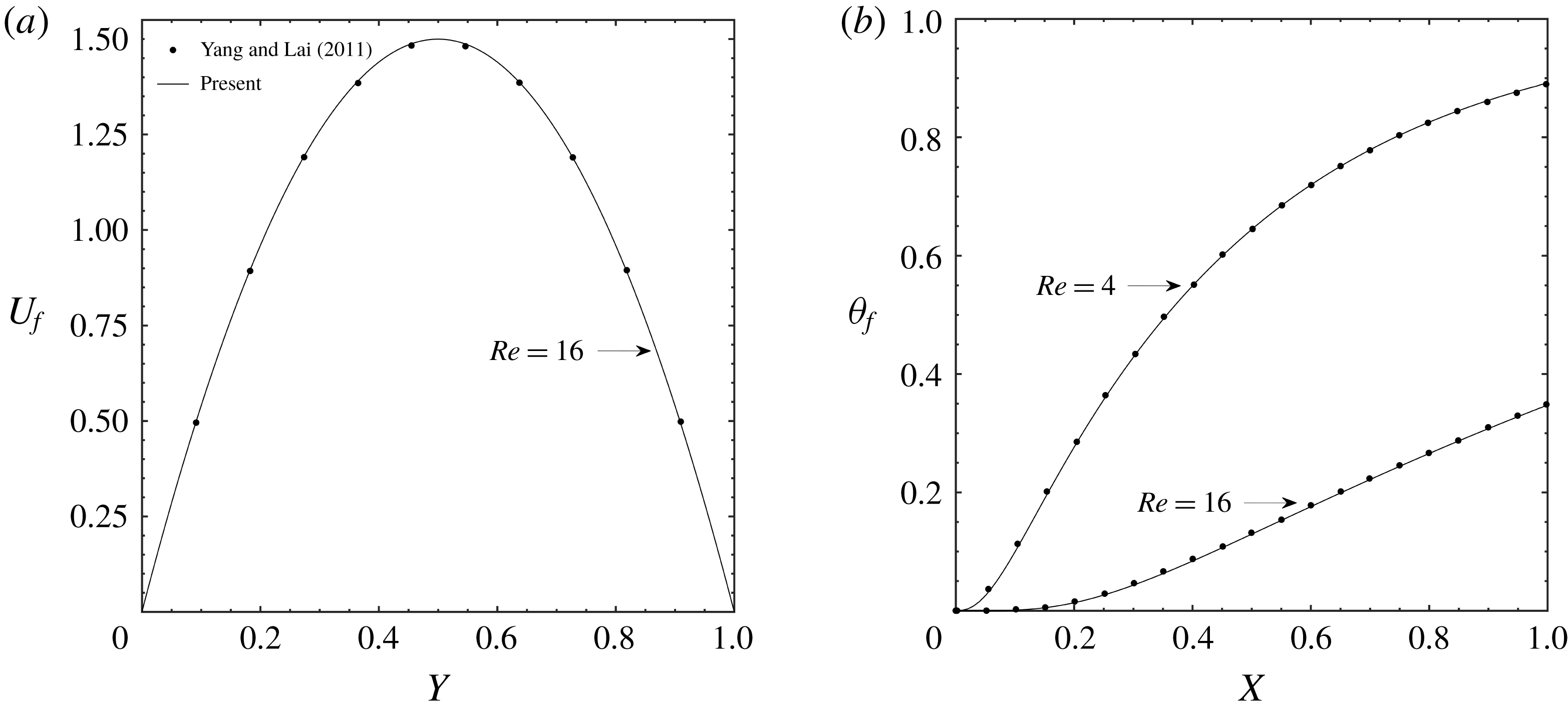
In order to verify our computations, the hydrodynamic and heat transfer characteristics (excluding Brownian motion effects) of an alumina–water nanofluid flowing in a microchannel with a rectangular cross-section are compared to the low-Reynolds-number results obtained with lattice-Boltzmann by Yang & Lai (Reference Yang and Lai2011). The top and bottom surfaces of the microchannel are maintained at a fixed temperature
 $T_{h}$
. Alumina particles size and volume fraction are 47 nm and 4 %, the channel has a
 $60\times 600~\unicode[STIX]{x03BC}\text{m}$
height and length, and the wall and fluid-inlet temperatures are respectively set to 333 K and 295 K. Figure 4(a) shows the non-dimensional velocity profile across the channel height at the channel outlet for
 $Re=16$
. Figure 4(b) shows the non-dimensional temperature profile along the channel length at the channel centre for
 $Re=4$
and
 $Re=16$
. As seen from the figure, there is a close agreement between present model results and that of Yang & Lai (Reference Yang and Lai2011).
Comparison of (a) non-dimensional velocity profile across the channel height at the channel outlet and (b) non-dimensional temperature profile along the channel length at the channel centre using the present model and published results.

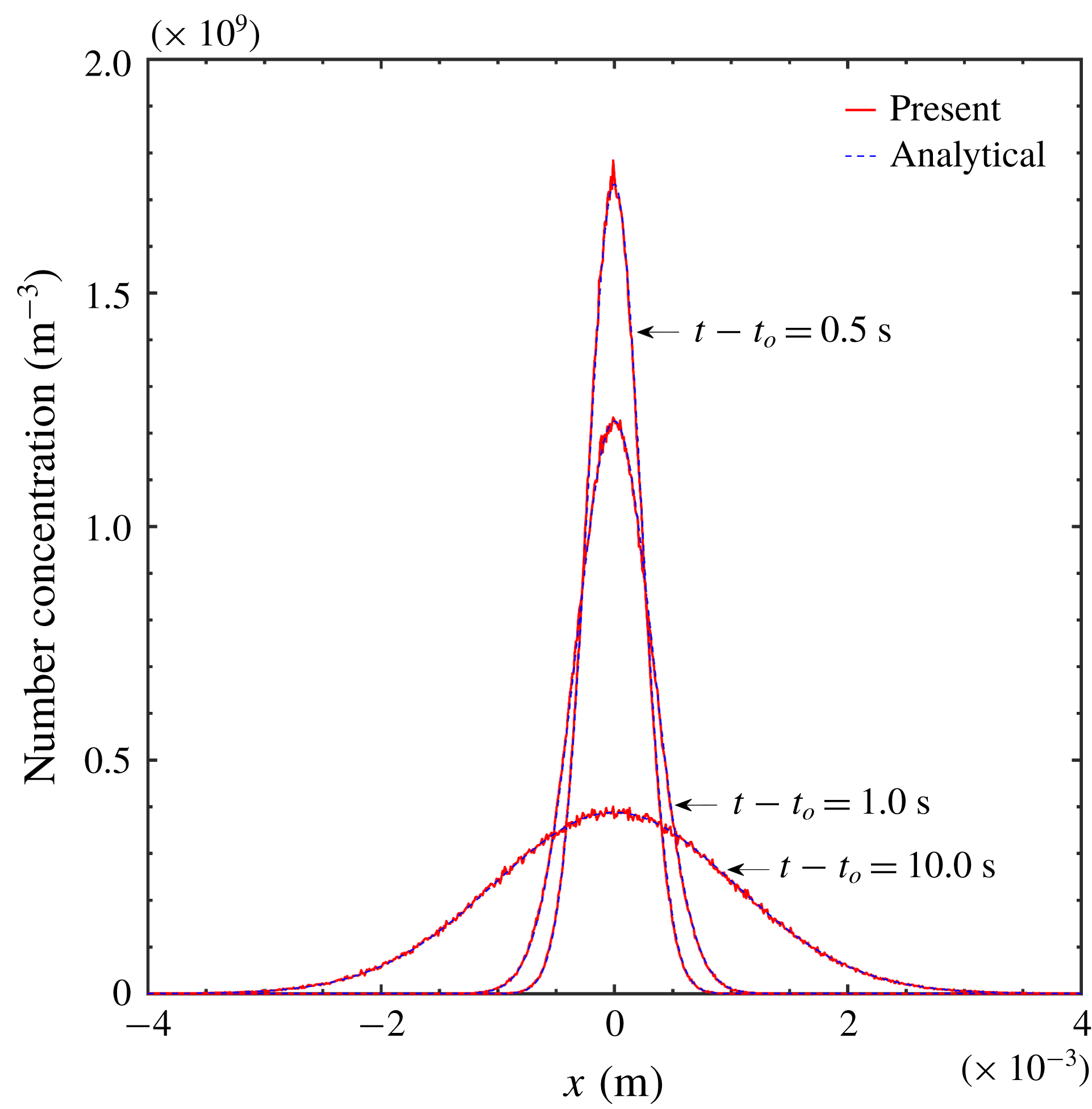
In order to verify the numerical implementation of the Brownian motion, the concentration profiles of nanoparticles allowed to freely diffuse under the influence of the random Brownian force and the systematic drag force in a stagnant fluid are computed and shown in figure 5. In figure 5, the computed concentration profiles are compared to the exact analytical solution of the diffusion equation for the case of an instantaneous source in an infinite medium, expressed as (Crank Reference Crank1975)
 $$\begin{eqnarray}c(t,x)=\frac{N_{p,0}}{\unicode[STIX]{x0394}y\unicode[STIX]{x0394}z(4\unicode[STIX]{x03C0}D_{B}(t-t_{0}))^{1/2}}\exp \left(\frac{-(x-x_{0})^{2}}{4\unicode[STIX]{x03C0}D_{B}(t-t_{0})}\right),\end{eqnarray}$$
where a total number
 $N_{p,0}$
of 1 000 000 particles with diameters of 10 nm have been released at time
 $t_{0}$
. The figure shows close agreement between numerical and analytical results. For relatively long simulation times (
 ${\sim}>0.5$
s), as shown in figure 5, it was found that the particle integration time step
 $\unicode[STIX]{x0394}t_{p}$
has no effect on the particle concentration distribution, while as the total simulation time becomes shorter, the condition on the maximum usable
 $\unicode[STIX]{x0394}t_{p}$
value becomes increasingly restrictive. Thus, in order to avoid any restrictions on
 $\unicode[STIX]{x0394}t_{p}$
(and the associated computational costs), all simulations hereinafter are run well within steady-state regime.
Comparison of particle concentration profiles after different total simulation times using the present model and the exact analytical solution of the diffusion equation.

Brownian motion could be described, according to timescale, within a Ballistic regime or a diffusive regime. In the ballistic regime (
 $t\ll \unicode[STIX]{x1D70F}_{m}$
), Brownian motion is dominated by particle inertia, whereas in the diffusive regime (
 $t\gg \unicode[STIX]{x1D70F}_{m}$
), Brownian motion is dominated by collisions with fluid molecules. Thus, and in order to determine which of the two Brownian motion regimes is relevant to our model, numerically generated mean-square displacement (MSD) results based on the Brownian force model adopted in the present study and the alternative Brownian force model proposed by Dong et al. (Reference Dong, Zheng, Zhang, Wu and Shen2014) are compared with analytical relations for the MSD in the ballistic and diffusive Brownian motion regimes. The alternative Brownian force expression proposed by Dong et al. (Reference Dong, Zheng, Zhang, Wu and Shen2014) is based on a modified Brownian motion spectral intensity expressed as
 $2R_{s}\unicode[STIX]{x1D705}_{B}T_{f}\unicode[STIX]{x1D6FE}/m^{\ast }$
, where
 $\unicode[STIX]{x1D6FE}=3\unicode[STIX]{x03C0}\unicode[STIX]{x1D707}_{f}D_{p}/m_{p}$
,
 $R_{s}=[\unicode[STIX]{x1D6FE}^{2}t^{2}+2\exp (-\unicode[STIX]{x1D6FE}t)-\exp (-2\unicode[STIX]{x1D6FE}t)-1]/[2\unicode[STIX]{x1D6FE}t+4\exp (-\unicode[STIX]{x1D6FE}t)-\exp (-2\unicode[STIX]{x1D6FE}t)-3]$
and
 $m^{\ast }=m_{p}+m_{f}/2$
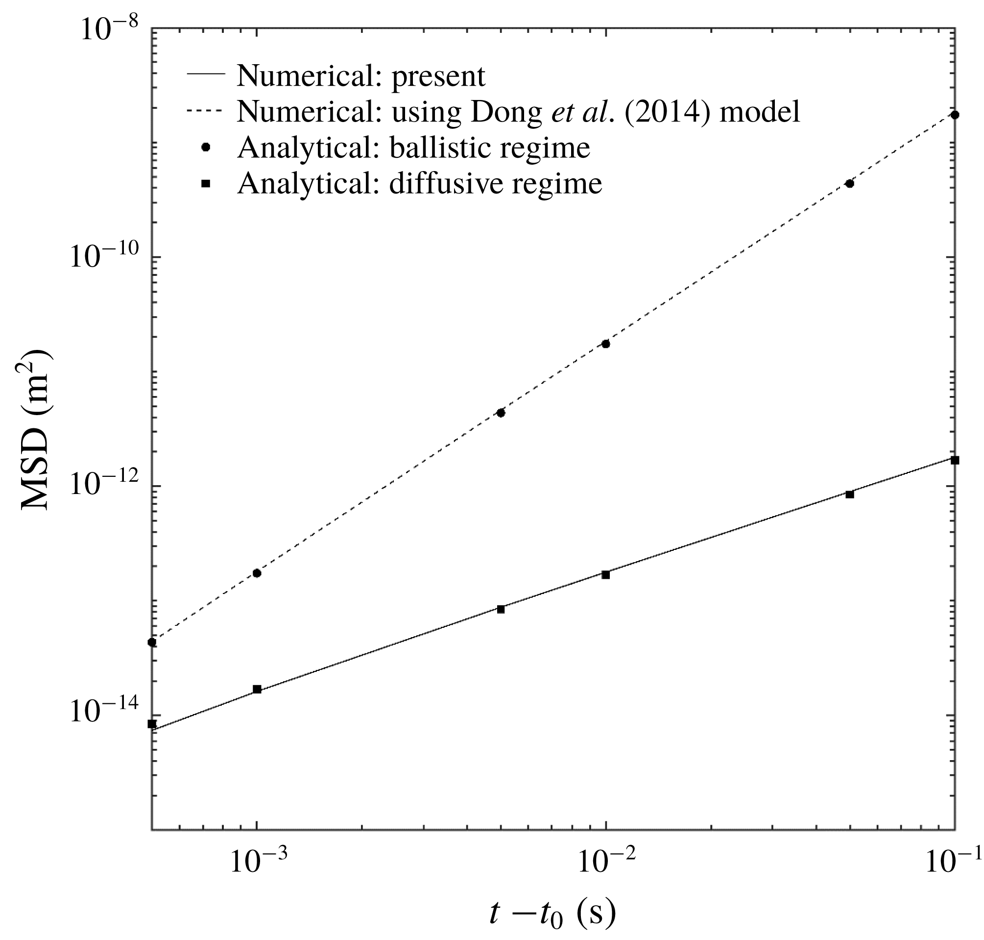
. The comparison results are shown in figure 6 for the case of
 $2.79~\unicode[STIX]{x03BC}\text{m}$
silica particles (at thermal equilibrium in air) using different total simulation times, all of which are well within the diffusive Brownian motion regime (i.e.
 $t\gg \unicode[STIX]{x1D70F}_{m}=4.85\times 10^{-5}~\text{s}$
). The figure shows that, although all considered total simulation times are within the diffusive Brownian motion regime, numerical results generated using the Dong et al. (Reference Dong, Zheng, Zhang, Wu and Shen2014) Brownian force model deviate from the diffusive regime MSD analytical relation, expressed as
 $2D_{B}(t-t_{0})$
, and instead follow the ballistic regime MSD analytical relation, expressed as
 $(6\unicode[STIX]{x1D705}_{B}T_{f}/\unicode[STIX]{x03C0}\unicode[STIX]{x1D70C}_{p}D_{p}^{3})(t-t_{0})^{2}$
. This is in contrast to the present model results that correctly follow the diffusive regime MSD analytical relation.
Comparison of MSDs within the diffusive regime
 $(t-t_{0}\gg \unicode[STIX]{x1D70F}_{m}=4.85\times 10^{-5}~\text{s})$
for numerical results generated using the adopted Brownian force model, numerical results generated using the Dong et al. (Reference Dong, Zheng, Zhang, Wu and Shen2014) Brownian force model and analytical relations for MSD in the ballistic and diffusive Brownian motion regimes.

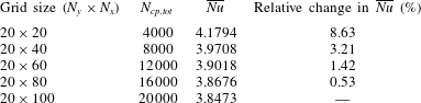
Grid-independence test showing the total number of computational particles.
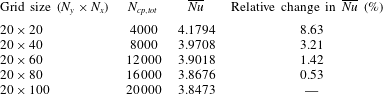
Finally, in order to ensure a grid-independent solution, the effect of spatial grid size on
 $\overline{Nu}$
is shown in table 2 for the case of
 $D_{p}=20~\text{nm}$
,
 $Re=10$
,
 $r=1.0$
and
 $L/H=100$
. It is important to note that since the number of computational particles in the Eulerian–Lagrangian computational algorithm is set to ten times the total number of Eulerian grid cells in this study (§ 2.3), the number of computational particles increases as the Eulerian grid is refined.
5 Results and discussion
5.1 Nanoparticle lateral migration
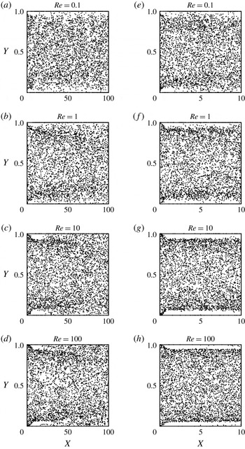
In figure 7, the spatial distribution of a sample of nanoparticles within the channel is shown for four different
 $Re$
values. Figures 7(e)–7(h) are a close-up at the entrance of the channel (first 10 % of total channel length) for the same
 $Re$
values. The figure shows that the distribution is highly non-uniform in the vicinity of the walls, especially for relatively high
 $Re$
values, indicating the inaccuracy of assuming a homogeneous particle distribution in modelling of nanofluid systems. This is unlike the core region of the channel, where nanoparticles distribution is relatively more uniform. Moreover, the non-uniform spatial distribution of nanoparticles in the channel leads to spatially non-uniform nanofluid thermophysical properties, as opposed to the spatially uniform effective nanofluid properties predicted by single-phase models.
Nanoparticle spatial distribution within the channel
 $(\unicode[STIX]{x1D719}_{p}=0.1\,\%,r=0.995)$
for (a–d) different Reynolds numbers and (e–h) a close-up at the entrance of the channel (first 10 % of total channel length) for the same Reynolds numbers.

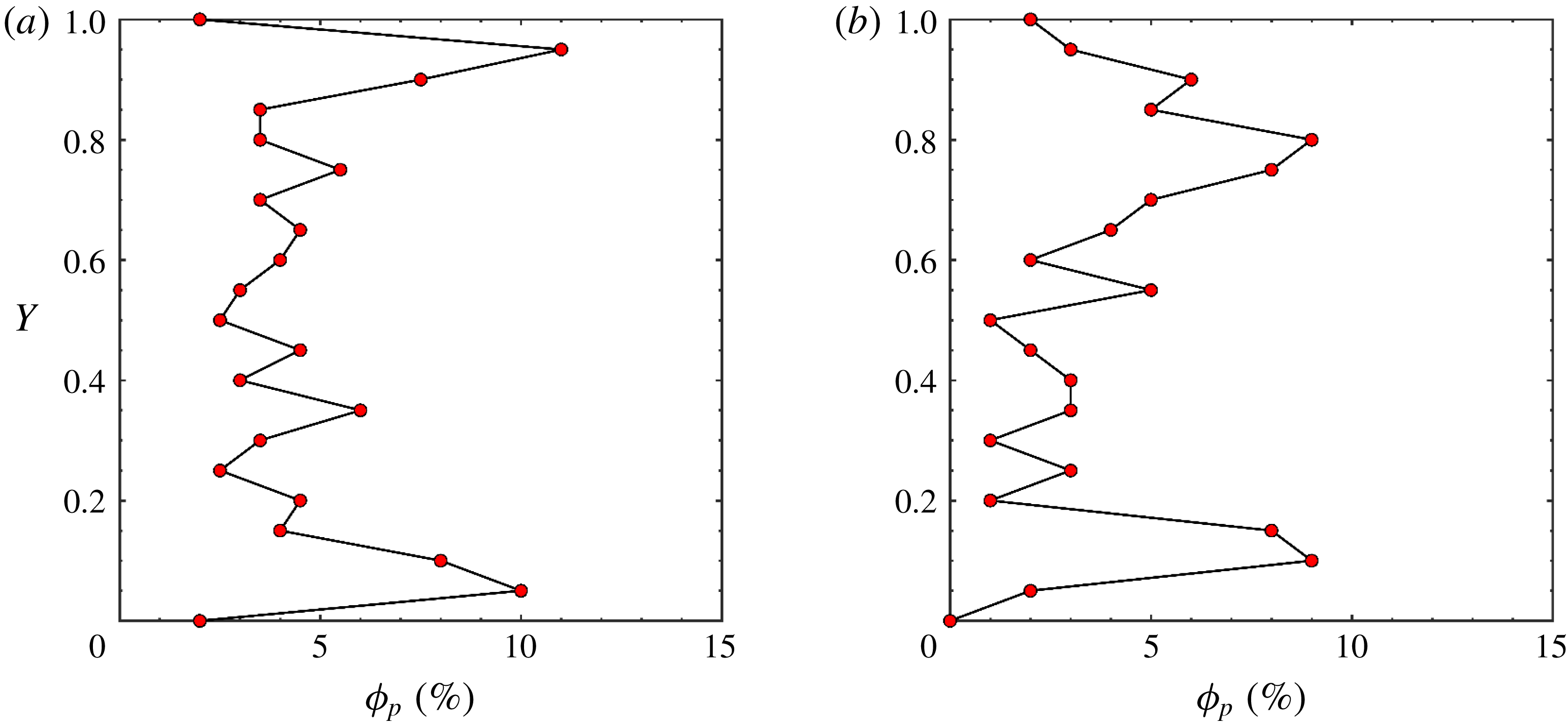
Since particles tend to migrate from high shear rate and high temperature gradient regions to low shear rate and low temperature gradient regions, nanoparticles rapidly migrate away from the vicinity of the walls where shear rate and temperature gradient are highest. This results in a low particle concentration depletion region near the walls, accompanied by the formation of a high particle concentration accumulation region between the wall and channel core, more towards the wall. These nanoparticle depletion and accumulation regions are illustrated in figure 8, where local nanoparticle volume fractions across the channel height are shown at the inlet and outlet of the channel for
 $Re=1$
. The high shear rate and temperature gradient near the walls result in a continuous flux of particles that accumulate in a region between the wall and channel core. Due to the resulting concentration gradient, diffusion of particles from the accumulation region takes place. However, the shear-rate-induced and temperature-gradient-induced fluxes (away from the walls) are higher than the concentration-induced flux (away from the accumulation region), resulting in a depletion region accompanied by an accumulation region rather than only a depletion region. It is worthy of mention that our observations regarding the non-uniform nanoparticle distribution and the formation of particle depletion and accumulation layers have not been previously reported in the nanofluid literature. This is largely attributed to the fact that the majority of works based on alternative modelling techniques (e.g. single-phase models) have inaccurately assumed nanoparticles to be homogeneously distributed within the channel.
Local particle volume fraction across the channel height at (a) the inlet and (b) outlet of the channel showing nanoparticle depletion and accumulation regions for
 $\mathit{Re}=1$
,
 $r=1.0$
and
 $\unicode[STIX]{x1D719}_{p}=5\,\%$
.

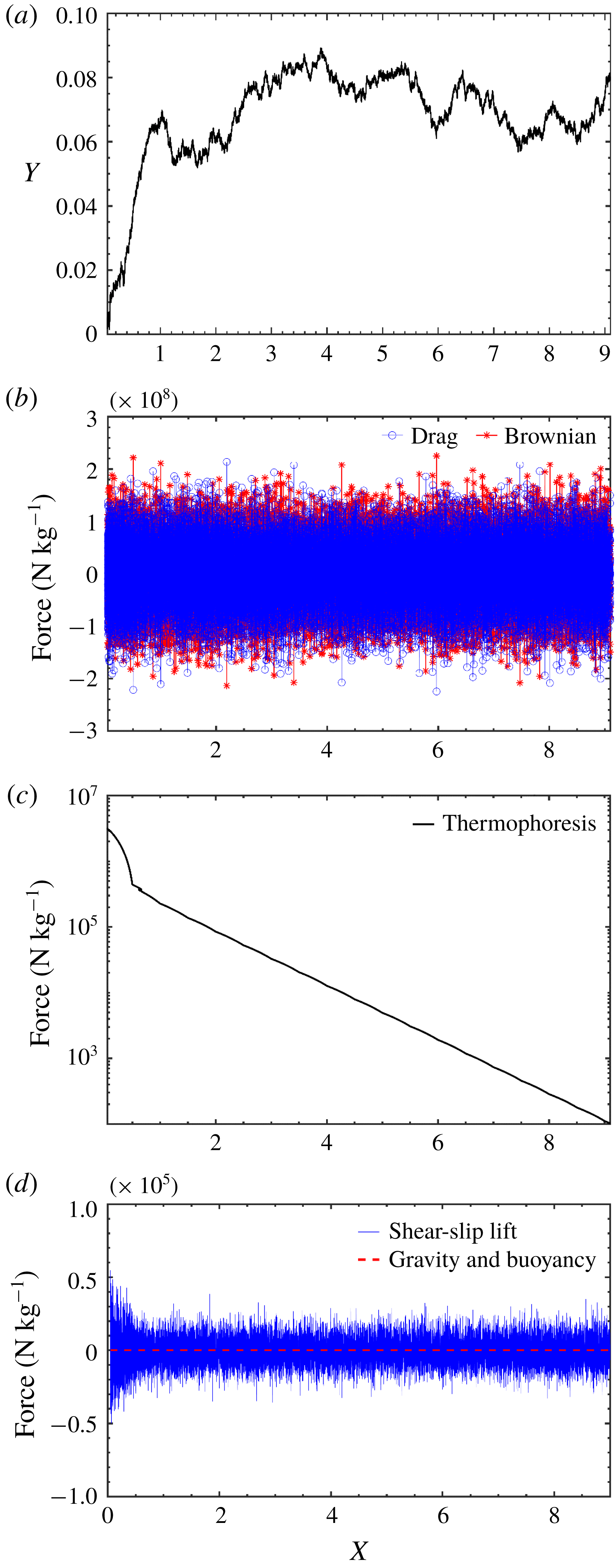
The depletion and accumulation regions start to form in the developing region of the flow where shear rate and temperature gradient near the walls are highest. This is shown in figure 9 where the history of the trajectory and transverse forces acting on a sample nanoparticle is shown for
 $Re=1$
. The figure shows that the magnitude of the thermophoretic and slip-shear-induced lift transverse forces are highest in the developing region of the microchannel. The figure also shows that drag and Brownian transverse forces are of the same order of magnitude, whereas the thermophoretic transverse force spans several orders of magnitude due to the drop in temperature gradient normal to the walls along the channel length. Gravity and buoyancy body forces are negligible for the case of nano-sized particles. In contrast to the fully continuous Eulerian–Eulerian approach, an advantage of our transient Eulerian–Lagrangian approach is that it provides access to the history of nanoparticle dispersion and trajectory as well as the relative importance of transverse forces acting on a nanoparticle, as shown in figure 9. Such information provides valuable and novel physical insights into the dynamics of fluid–particle and particle–wall interactions, which allowed us to observe and justify the phenomenon of particle depletion and accumulation regions formation in the microchannel system.
History of the (a) trajectory and (b–d) transverse specific forces (
 $\text{N}~\text{kg}^{-1}$
) acting on a sample nanoparticle along the channel length for
 $\mathit{Re}=1$
,
 $D_{p}=20~\text{nm}$
,
 $r=1.0$
and
 $\unicode[STIX]{x1D719}_{p}=5\,\%$
.

At relatively low
 $Re$
, the particle distribution near the walls gradually flattens in the streamwise direction, as seen from figures 7(e,f) and 8, due to the effect of random Brownian motion that smooths particle concentration gradients in nano-sized particle systems, whereas for relatively higher
 $Re$
values, the magnitude of shear rate increases while the relative effect of Brownian motion decreases, leading to more particle migration away from channel walls (figure 7
g,h). Moreover, at low
 $Re$
, the boundary layer is thick while the entrance length is short. This results in the thick but short particle depletion region near the walls, as seen from figure 7(a,b,e,f). On the other hand, at high
 $Re$
, the boundary layer is thin while the entrance length is long. This results in the thin but long particle depletion region near the walls, as seen from figure 7(c,d,g,h).
Our results indicate that there exists a close relation between nanoparticle dispersion and developing zone length. The onset of the observed nanoparticle depletion and accumulation layers takes place in the developing region of the microchannel, resulting in the highly non-uniform spatial particle distribution near channel walls. This is attributed to the fact that the relative magnitude of slip-shear-induced lift and thermophoretic transverse forces acting on nanoparticles are respectively highest in the hydrodynamically and thermally developing regions of the nanofluid flow, where shear rate and temperature gradient near the walls are highest. Moreover, as Reynolds number decreases, the boundary layer becomes thicker and the entrance length becomes shorter, leading to a thicker and shorter nanoparticle depletion region near channel walls. These results are an important indication that neglecting the effects of the developing region altogether by assuming the nanofluid flow to be fully developed throughout the channel, as commonly done in the nanofluid literature, can lead to erroneous results and the missing of important phenomena such as the particle depletion and accumulation regions reported in this work.
5.2 Reynolds number and nanoparticle loading effects on heat transfer
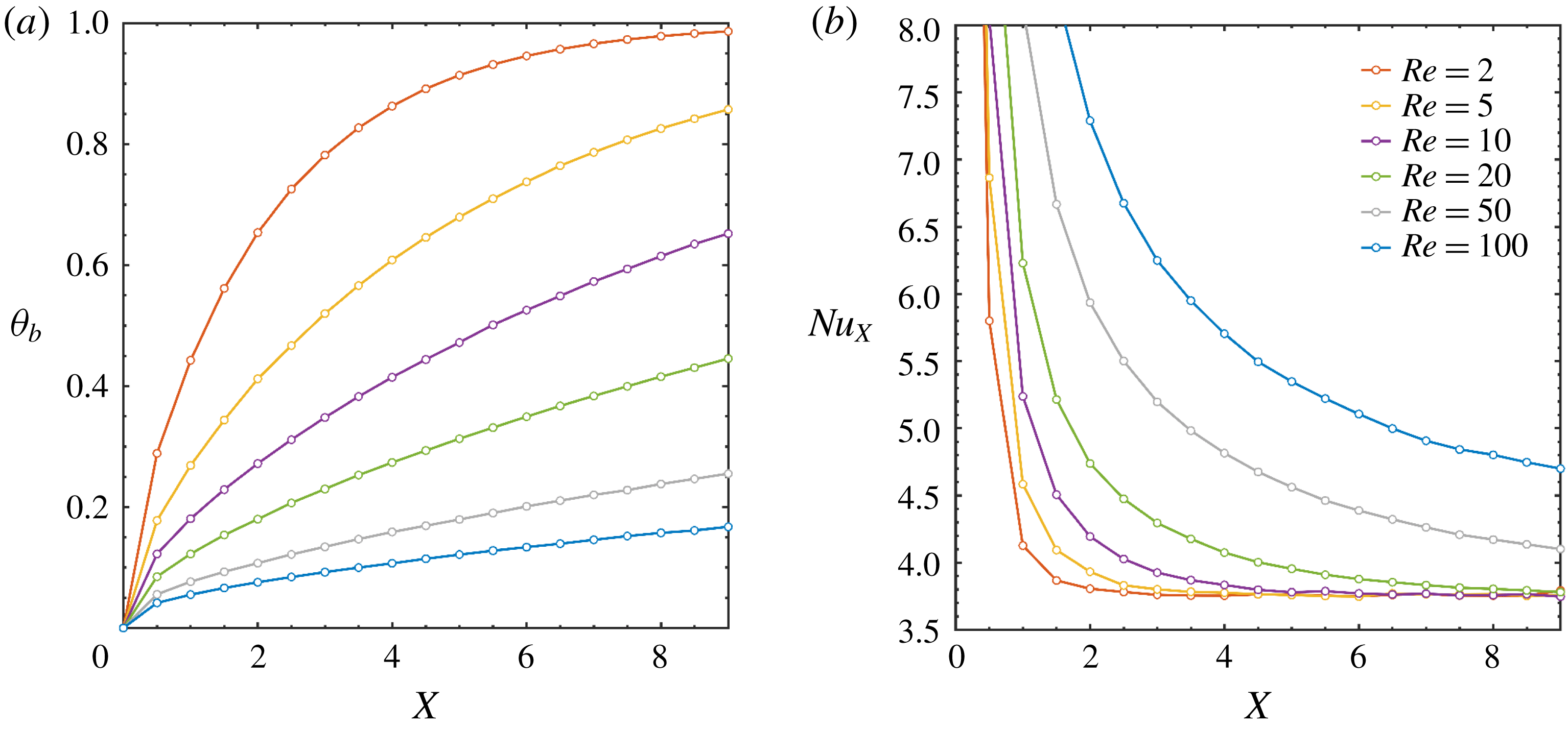
In figure 10, the effects of
 $Re$
on local bulk fluid temperature
 $\unicode[STIX]{x1D703}_{b}$
and bottom wall local Nusselt number
 $Nu_{x}$
along the channel length are shown for
 $\unicode[STIX]{x1D719}_{p}=2\,\%$
, where
 $\unicode[STIX]{x1D703}_{b}$
is expressed as
 $$\begin{eqnarray}\unicode[STIX]{x1D703}_{b}(X)=\frac{\displaystyle \int _{0}^{1}U_{f}(X,Y)\unicode[STIX]{x1D703}_{f}(X,Y)\,\text{d}Y}{\displaystyle \int _{0}^{1}U_{f}(X,Y)\,\text{d}Y}.\end{eqnarray}$$
As seen from the figure, an increase in
 $Re$
results in lower bulk fluid temperatures and a corresponding enhancement of convective heat transfer and Nusselt number from channel walls to the fluid due to the larger temperature gradient normal to the channel wall. Moreover, bulk fluid temperature increases with axial distance as a result of augmented heat transfer along channel length, as opposed to the Nusselt number which decreases with axial distance due to the smaller temperature gradient normal to the channel walls. Figure 10(b) also shows that for a higher
 $Re$
, there are more gradual changes in the Nusselt number along the channel length. This is attributed to the fact that the fully developed entrance length linearly increases with
 $Re$
, which results in a larger portion of the flow being in the developing region, where temperature gradient normal to the walls changes less rapidly in the streamwise direction. Figure 10(b) shows that heat transfer enhancement rapidly decreases with increasing distance from the entrance region. Therefore, in order to maximize heat transfer enhancement using nanofluids during the low-Reynolds-number flows at hand, it is important to design a microchannel such that the flow remains in the developing region for as long as possible in such flows. The dispersion of nanoparticles in a pure fluid is proposed as a way to increase the thermal entrance length for a given, relatively low value of the Reynolds number.
Effect of Reynolds number on (a) bulk fluid temperature and (b) bottom wall local Nusselt number across the channel length.

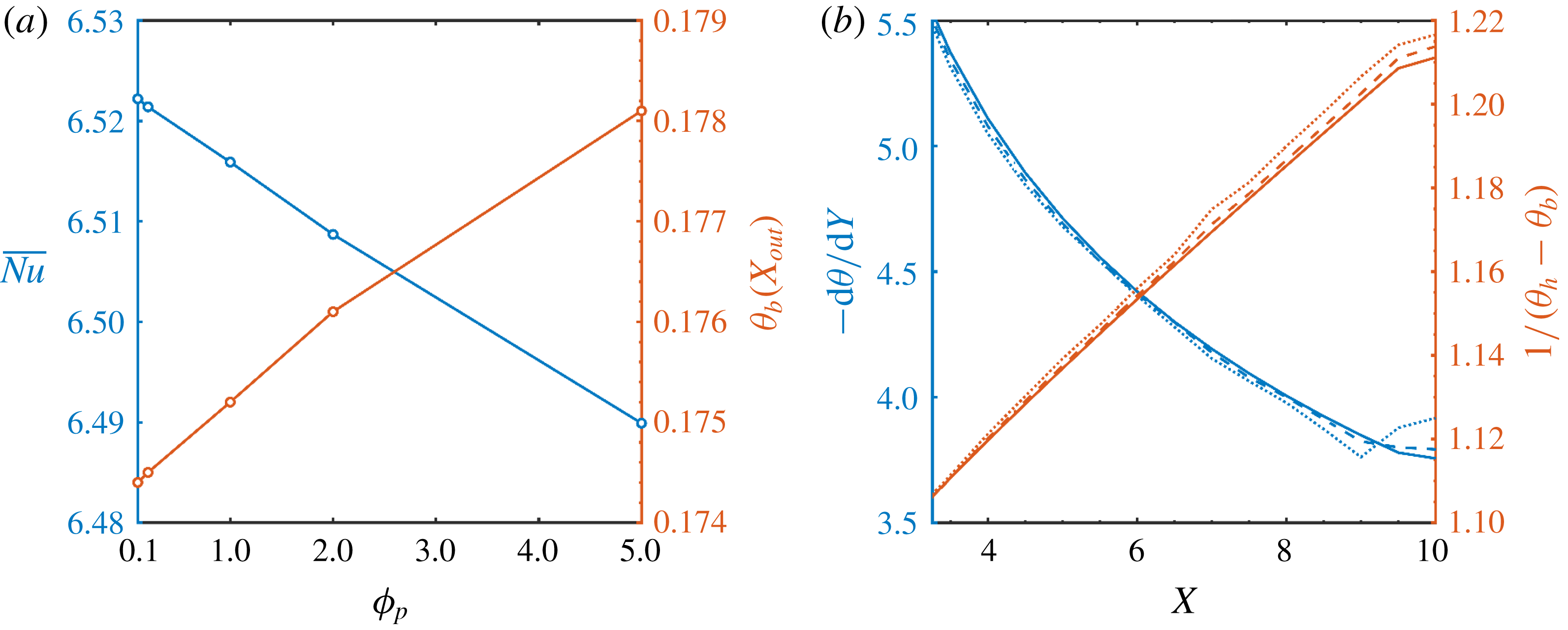
Effect of changing particle volume fraction (
 $\mathit{Re}=100$
) on (a) average Nusselt number and bulk fluid temperature at the channel exit and (b) the bulk fluid temperature term and normal temperature gradient term in the definition of local Nusselt number (solid lines:
 $\unicode[STIX]{x1D719}_{p}=0\,\%$
; dashed lines:
 $\unicode[STIX]{x1D719}_{p}=2\,\%$
; dotted lines:
 $\unicode[STIX]{x1D719}_{p}=5\,\%$
).

Figure 11(a) shows the effects of varying particle volume fraction on
 $\overline{Nu}$
and bulk fluid temperature
 $\unicode[STIX]{x1D703}_{b}$
at the channel exit for
 $Re=100$
. Increasing the particle volume fraction results in a higher bulk fluid temperature as a result of the improved heat transfer from the hot walls to the nanofluid flow. Figure 11(a) also shows that there is an inversely proportional relation between particle volume fraction and
 $\overline{Nu}$
. This negative effect of
 $\unicode[STIX]{x1D719}_{p}$
on
 $\overline{Nu}$
could be justified using figure 11(b). In figure 11(b), the effects of varying particle volume fraction on the
 $-\unicode[STIX]{x2202}\unicode[STIX]{x1D703}/\unicode[STIX]{x2202}Y|_{X}$
term and the
 $1/[\unicode[STIX]{x1D703}_{h}-\unicode[STIX]{x1D703}_{b}(x)]$
term in the definition of
 $Nu_{x}$
are shown (notice that
 $\unicode[STIX]{x1D703}_{h}=1$
, by definition). Since an increase in
 $\unicode[STIX]{x1D719}_{p}$
results in an increase in
 $\unicode[STIX]{x1D703}_{b}$
, as established from figure 11(a), the end result is an increase in the
 $1/[\unicode[STIX]{x1D703}_{h}-\unicode[STIX]{x1D703}_{b}(x)]$
term. On the other hand, since
 $\unicode[STIX]{x1D703}_{b}$
increases due to the enhanced heat transfer at higher
 $\unicode[STIX]{x1D719}_{p}$
values, the temperature gradient normal to the wall
 $-\unicode[STIX]{x2202}\unicode[STIX]{x1D703}/\unicode[STIX]{x2202}Y|_{X}$
drops with an increase in
 $\unicode[STIX]{x1D719}_{p}$
. This ultimately results in a drop in
 $Nu_{x}$
and
 $\overline{Nu}$
with
 $\unicode[STIX]{x1D719}_{p}$
, as shown in figure 11(a), as the rise in the
 $1/[\unicode[STIX]{x1D703}_{h}-\unicode[STIX]{x1D703}_{b}(x)]$
term with
 $\unicode[STIX]{x1D719}_{p}$
is slower than the drop in the
 $-\unicode[STIX]{x2202}\unicode[STIX]{x1D703}/\unicode[STIX]{x2202}Y|_{X}$
term with
 $\unicode[STIX]{x1D719}_{p}$
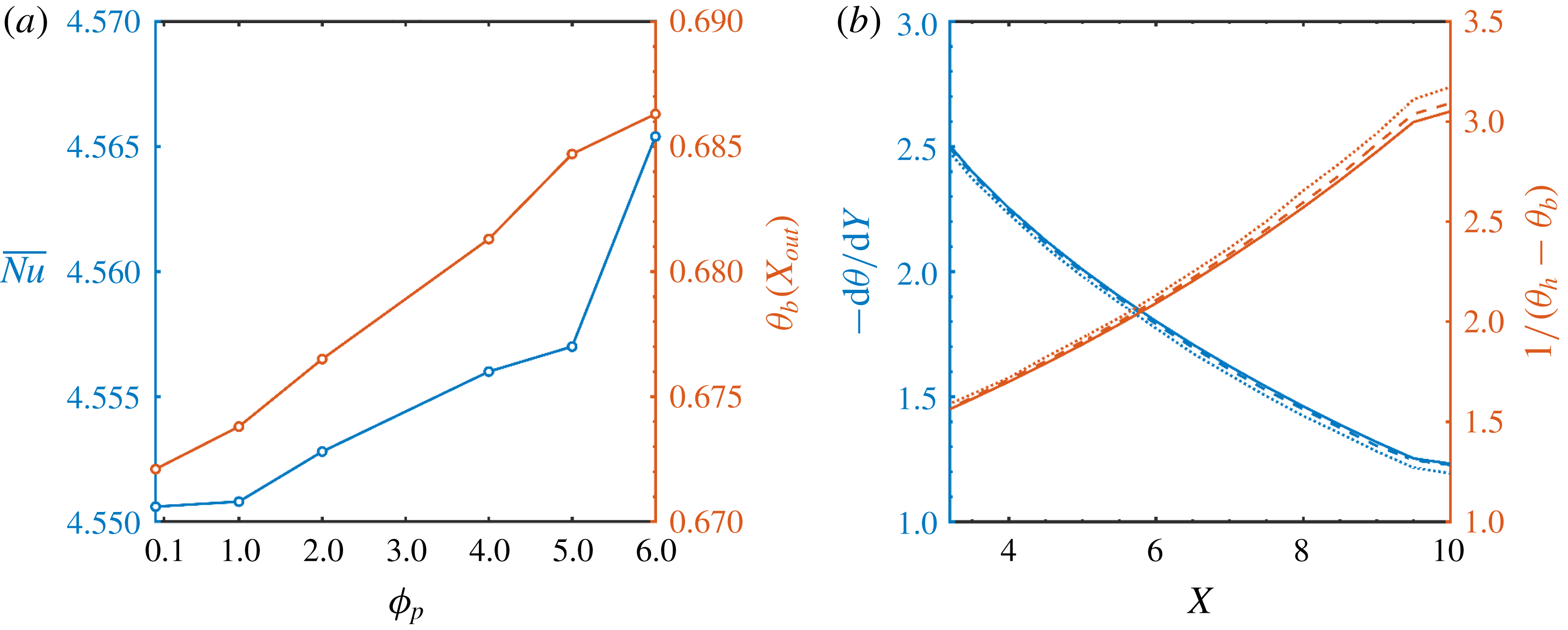
. While for a lower Reynolds number value of 10, figure 12(a) shows that
 $\overline{Nu}$
increases with
 $\unicode[STIX]{x1D719}_{p}$
which is a result of the rise in the
 $1/[\unicode[STIX]{x1D703}_{h}-\unicode[STIX]{x1D703}_{b}(x)]$
term dominating over the drop in the
 $-\unicode[STIX]{x2202}\unicode[STIX]{x1D703}/\unicode[STIX]{x2202}Y|_{X}$
term with
 $\unicode[STIX]{x1D719}_{p}$
, as shown in figure 12(b). This change of behaviour could be attributed to the effect of nanoparticles on increasing the thermal entrance length at lower
 $Re$
. By comparing figures 11(a) and 12(a), we conclude that there exists a critical Reynolds number of enhancement, beyond which the addition of nanoparticles does not increase the heat transfer coefficient from channel walls to bulk fluid. By virtue of considering developing region effects and the discrete nature of nanoparticles using our Eulerian–Lagrangian approach, our novel observation on the existence of a critical Reynolds number of enhancement in forced-convection nanofluid-based microchannel systems can elucidate contradictory results previously reported in the nanofluid literature regarding whether nanoparticle dispersion enhances or diminishes heat transfer in microchannel heat exchangers.
Effect of changing particle volume fraction (
 $\mathit{Re}=10$
) on (a) average Nusselt number and bulk fluid temperature at the channel exit and (b) the bulk fluid temperature term and normal temperature gradient term in the definition of local Nusselt number (solid lines:
 $\unicode[STIX]{x1D719}_{p}=0\,\%$
; dashed lines:
 $\unicode[STIX]{x1D719}_{p}=2\,\%$
; dotted lines:
 $\unicode[STIX]{x1D719}_{p}=5\,\%$
).

5.3 Forces acting on the dispersed phase and particle size effects
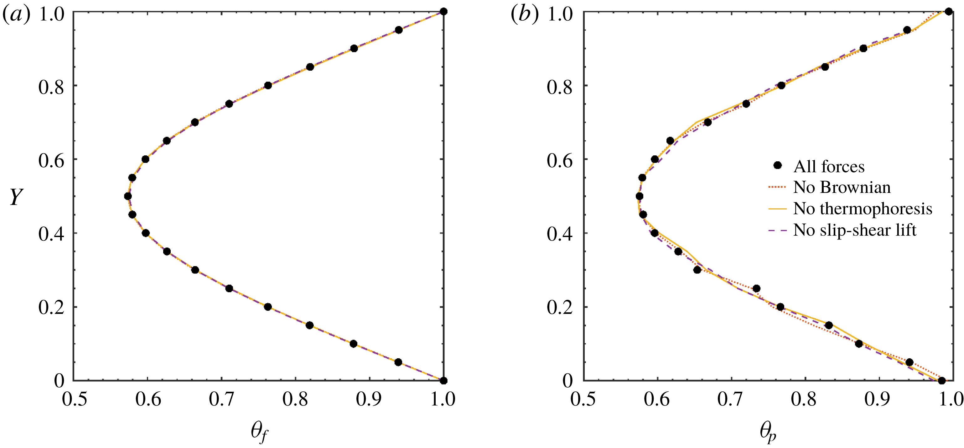
Regarding the effect of forces acting on the fluid phase, figure 13(a) shows the effect of including all forces, then excluding in turn the Brownian force, the thermophoretic force and the slip-shear-induced transverse lift force, on the temperature distribution at the channel outlet using
 $Re=10$
and
 $\unicode[STIX]{x1D719}_{p}=2\,\%$
. The figure shows that including or excluding these three forces has a negligible effect on the fluid phase. Regarding the particle phase, figure 13(b) shows that Brownian, thermophoretic and slip-shear-induced lift forces have a small effect on particle-phase temperature distribution. This is due to the dominant effect of drag force relative to all other forces for nano-sized particles.
Effect of Brownian, thermophoretic and slip-shear-induced lift forces on (a) fluid-phase and (b) particle-phase temperature distributions at channel outlet.

Nonetheless, it is found that Brownian motion has a dominant role within the vicinity of channel walls. In fact, Brownian motion is the main deposition mechanism for nano-sized particles, as the percentage of deposited particles drops from 1.85 % to 0 % when Brownian force is excluded under the current operation conditions
 $(r=0.99)$
. Thermophoresis also has a major effect on particle migration from the hot channel walls towards the cold channel centre, as the percentage of deposited particles rises from 1.85 % to 2.58 % when thermophoretic force is excluded under the current operation conditions
 $(r=0.99)$
. This is due to the role of thermophoresis in repelling nanoparticles along the temperature gradient away from the hot channel walls, thus decreasing their chances of deposition. In fact, since the temperature gradient normal to the walls is highest in the entrance region of the channel, nanoparticle deposition gradually increases along the channel length, where it reaches a maximum at the channel outlet and a minimum at the channel inlet. Thus, we conclude that Brownian and thermophoretic forces have opposing effects on the deposition of nanoparticles in confined nanofluid flows with constant-temperature walls. This new and important result regarding nanoparticle deposition is a result of accurately modelling particle–wall and fluid–particle interactions in the developing and developed regions of the flow. Such results are normally not accessible using alternative single-phase and Eulerian–Eulerian models.
Effect of particle size on (a) particle deposition percentage and (b) average Nusselt number.

As seen in figure 14(a) for
 $\unicode[STIX]{x1D719}_{p}=1\,\%$
and
 $Re=10$
, when the particle size increases, the number of deposited particles decreases. This is attributed to the smaller relative magnitude of random Brownian motion for larger particle sizes, which is the key mechanism behind nanoparticle deposition and motion slip fluctuations between fluid and nanoparticle phases. Nonetheless, as seen from figure 14(b), the average Nusselt number slightly drops with increased particle size. This could be attributed to two reasons. The first has to do with two opposing effects on nanofluid viscosity. It is generally recognized that as the nanoparticle size increases, so does the nanofluid viscosity. A higher nanofluid viscosity results in a larger thermal boundary layer and a lower rate of convective heat transfer. On the other hand, when particle migration effects in the microchannel are taken into account, larger particle sizes result in a larger particle depletion region near channel walls due to the weaker homogenizing effects of Brownian diffusion. A large particle depletion region leads to a lower nanofluid viscosity in the region adjacent to channel walls. This, in turn, results in a smaller thermal boundary layer and a higher rate of convective heat transfer. This trade-off relation between particle size and convective heat transfer results in the observed small drop in Nusselt number with an increase in nanoparticle size, as seen in figure 14(b). Although many authors have reported that an increase in nanoparticle size systematically results in a sharp drop in convective heat transfer rate, this could be attributed to ignoring lateral particle migration effects. As these effects are captured using our Eulerian–Lagrangian approach, an important trade-off is revealed between particle size and local nanofluid viscosity near channel walls, which ultimately results in the marginal drop in Nusselt number with increased particle size. The second reason has to do with averaging the local Nusselt number over relatively long microchannels. In particular, it is generally known that in the fully developed region, heat transfer enhancement by the effect of the dispersed nanoparticles is small relative to enhancement in the developing entrance region. When relatively long microchannels are used, such as the case in this study, most of the flow will be in the fully developed region and the overall effect of the entrance region will be minimal. As a result, any enhancement in heat transfer rate in the short entrance region when smaller nanoparticles are used will not be well-reflected in the average Nusselt number of a long microchannel, which is consistent with our results in figure 14(b). Regarding the effect of
 $Re$
on nanoparticle deposition, it is found that the deposition percentage drops to 1 % at approximately
 $Re=100$
, as shown in figure 15, for the current study conditions. The figure shows that as
 $Re$
increases, the deposition percentage decreases. This is attributed to the weaker effect of Brownian diffusion at relatively higher
 $Re$
values, where the depletion–accumulation phenomenon near channel walls becomes more dominant. The figure also shows that after
 $Re=1$
, nanoparticle deposition on channel walls starts to steeply decrease.
Effect of
 $Re$
on nanoparticle deposition percentage (
 $\unicode[STIX]{x1D719}_{p}=0.1\,\%$
,
 $D_{p}=20~\text{nm}$
,
 $r=0.995$
,
 $L/H=100$
).

6 Conclusions
Using a two-way coupled Eulerian–Lagrangian approach implemented via a transient in-house code, it was established that nanoparticle distribution is highly non-uniform in the vicinity of channel walls. This demonstrates the inaccuracy of assuming a homogeneous particle distribution in modelling of nanofluid microchannel systems. In particular, shear rate and thermophoresis played a key role in the lateral migration of nanoparticles and in the formation of depletion and accumulation regions near channel walls. These depletion and accumulation regions started to form in the developing region of the flow where shear rate and temperature gradient near the walls were highest. For relatively low
 $Re$
, nanoparticle distribution near the walls gradually flattened in the streamwise direction, due to the effect of random Brownian motion, whereas for relatively higher
 $Re$
, shear rate and temperature gradient effects dominated over Brownian motion, leading to higher particle non-uniformities in the vicinity of channel walls. Furthermore, convective heat transfer from channel walls to bulk fluid can improve or deteriorate with the addition of nanoparticles, depending on the flow Reynolds number. In fact, there exists a critical Reynolds number of enhancement, beyond which the addition of nanoparticles did not increase the heat transfer coefficient from channel walls to bulk fluid. This is closely related to the observed particle migration phenomenon, which can dramatically change the spatial distribution of the nanofluid thermophysical properties, especially for mini/microchannel geometries. Finally, it was established that Brownian motion and thermophoresis played a major role in nanoparticle deposition in microchannels. Brownian motion was the main deposition mechanism for nano-sized particles, whereas thermophoresis decreased the chances of particle deposition. In fact, due to diminishing thermophoresis, nanoparticle deposition gradually increased along the channel length and reached a maximum at the channel outlet.
Nomenclature
-
$A_{H}$
Hamaker constant
$\left(\text{J}\right)$
-
$B_{x},B_{y}$
Non-dimensional sum of body forces
-
$Bi$
Biot number,
$Bi=hD_{p}/6k_{p}$
-
$c$
Number concentration
$(\text{m}^{-3})$
-
$C$
Specific heat capacity
$(\text{J}~\text{kg}^{-1}~\text{K}^{-1})$
-
$C_{c}$
Cunningham slip correction factor
-
$C_{i}$
Fluid inertia correction factor
-
$D$
Diameter (m)
-
$D_{B}$
Corrected Brownian diffusivity
$(\text{m}^{2}~\text{s}^{-1})$
-
$D_{T}$
Thermophoretic diffusivity
$(\text{m}^{2}~\text{s}^{-1})$
-
$E$
Particle–wall van der Waals interaction potential (J)
-
$f_{C}$
Specific heat capacity ratio,
$f_{C}=C_{f}/C_{p}$
-
$f_{p}$
Parcel factor
-
$f_{\unicode[STIX]{x1D70C}}$
Density ratio,
$f_{\unicode[STIX]{x1D70C}}=\unicode[STIX]{x1D70C}_{f}/\unicode[STIX]{x1D70C}_{p}$
-
$Fr$
Froude number,
$Fr=u_{in}/\sqrt{gH}$
-
$g$
Gravitational acceleration,
$g=9.81~\text{m}~\text{s}^{-2}$
-
$h$
Convective heat transfer coefficient
$(\text{W}~\text{m}^{-2}~\text{K}^{-1})$
-
$H$
Channel height (m)
-
$k$
Thermal conductivity
$(\text{W}~\text{m}^{-1}~\text{K}^{-1})$
-
$Kn_{ch}$
Channel-based Knudsen number,
$Kn_{ch}=MFP_{f}/H$
-
$Kn_{p}$
Particle-based Knudsen number,
$Kn_{p}=MFP_{f}/D_{p}$
-
$K_{T}$
Thermophoresis parameter
-
$L$
Channel length (m)
-
$m$
Mass (kg)
-
$MFP$
Mean free path (m)
-
$\text{MSD}$
Mean-square displacement
$(\text{m}^{2})$
-
$N$
Number
-
$\overline{Nu}$
Average Nusselt number,
$\overline{Nu}=(1/(L/H))\int _{0}^{L/H}Nu_{x}\,\text{d}X$
-
$Nu_{p}$
Particle Nusselt number,
$Nu_{p}=hD_{p}/k_{f}$
-
$Nu_{x}$
Local Nusselt number,
$Nu_{x}=(-1/(\unicode[STIX]{x1D703}_{h}-\unicode[STIX]{x1D703}_{b}))(\unicode[STIX]{x2202}\unicode[STIX]{x1D703}/\unicode[STIX]{x2202}Y)|_{X}$
-
$Pe_{B}$
Brownian Péclet number,
$Pe_{B}=u_{in}H/D_{B}$
-
$Pe_{T}$
Thermophoretic Péclet number,
$Pe_{T}=u_{in}H/D_{T}$
-
$Pr$
Prandtl number,
$Pr=\unicode[STIX]{x1D707}_{f}C_{f}/k_{f}$
-
$r$
Normal coefficient of restitution
-
$Re$
Reynolds number,
$Re=u_{in}H/\unicode[STIX]{x1D708}_{f}$
-
$RE$
Relative error
-
$Re_{p}$
Particle relative Reynolds number,
$Re_{p}=(|u_{f}-u_{p}|D_{p})/\unicode[STIX]{x1D708}_{f}$
-
$Ri$
Richardson number,
$Ri=(g\unicode[STIX]{x1D6FD}_{f}(T_{h}-T_{c})H)/u_{in}^{2}$
-
$s_{pe}$
Particle energy source term
$(\text{K}~\text{s}^{-1})$
-
$S_{pe}$
Non-dimensional particle energy source term
-
$s_{pm}$
Particle momentum source term
$(\text{s}^{-2})$
-
$S_{pm}$
Non-dimensional particle momentum source term
-
$St$
Stokes number,
$St=\unicode[STIX]{x1D70F}_{m}/\unicode[STIX]{x1D70F}_{F}$
-
$St_{\unicode[STIX]{x1D703}}$
Thermal Stokes number,
$St_{\unicode[STIX]{x1D703}}=\unicode[STIX]{x1D70F}_{\unicode[STIX]{x1D703}}/\unicode[STIX]{x1D70F}_{F}$
-
$t$
Time (s)
-
$T$
Temperature (K)
-
$u,v$
Velocity
$(\text{m}~\text{s}^{-1})$
-
$U,V$
Non-dimensional velocity,
$U=u/u_{in}$
,
$V=v/u_{in}$
-
$u_{T},v_{T}$
Thermophoretic velocity
$(\text{m}~\text{s}^{-1})$
-
$v_{C}$
Particle capture velocity
$(\text{m}~\text{s}^{-1})$
-
$W$
Channel width (m)
-
$x,y$
Location (m)
-
$X,Y$
Non-dimensional location,
$X=x/H$
,
$Y=y/H$
-
$\forall$
Volume
$(\text{m}^{3})$













Greek letters
-
$\unicode[STIX]{x1D6FC}$
Thermal diffusivity
$(\text{m}^{2}~\text{s}^{-1})$
-
$\unicode[STIX]{x1D6FD}$
Thermal expansion coefficient
$(\text{K}^{-1})$
-
$\unicode[STIX]{x1D6FF}$
Zero-mean, unit-variance independent Gaussian random number
-
$\unicode[STIX]{x1D703}$
Non-dimensional temperature,
$\unicode[STIX]{x1D703}=(T-T_{c})/(T_{h}-T_{c})$
-
$\unicode[STIX]{x1D705}_{B}$
Boltzmann constant,
$\unicode[STIX]{x1D705}_{B}=1.38\times 10^{-23}~\text{J}~\text{K}^{-1}$
-
$\unicode[STIX]{x1D707}$
Dynamic viscosity
$(\text{kg}~\text{m}^{-1}~\text{s}^{-1})$
-
$\unicode[STIX]{x1D708}$
Kinematic viscosity
$(\text{m}^{2}~\text{s}^{-1})$
-
$\unicode[STIX]{x1D709}$
Particle-wall equilibrium separation distance (m)
-
$\unicode[STIX]{x1D70C}$
Density
$(\text{kg}~\text{m}^{-3})$
-
$\unicode[STIX]{x1D70E}$
Stefan–Boltzmann constant,
$\unicode[STIX]{x1D70E}=5.67\times 10^{-8}~\text{W}~\text{m}^{-2}~\text{K}^{-4}$
-
$\unicode[STIX]{x1D70F}$
Non-dimensional time,
$\unicode[STIX]{x1D70F}=u_{in}t/H$
-
$\unicode[STIX]{x1D70F}_{F}$
Fluid advection time (s)
-
$\unicode[STIX]{x1D70F}_{m}$
Particle momentum relaxation time (s)
-
$\unicode[STIX]{x1D70F}_{\unicode[STIX]{x1D703}}$
Particle thermal relaxation time (s)
-
$\unicode[STIX]{x1D719}$
Volume fraction
-
$\unicode[STIX]{x1D713}$
Stream function
$(\text{m}^{2}~\text{s}^{-1})$
-
$\unicode[STIX]{x1D6F9}$
Non-dimensional stream function,
$\unicode[STIX]{x1D6F9}=\unicode[STIX]{x1D713}/u_{in}H$
-
$\unicode[STIX]{x1D714}$
Vorticity
$(\text{s}^{-1})$
-
$\unicode[STIX]{x1D6FA}$
Non-dimensional vorticity,
$\unicode[STIX]{x1D6FA}=\unicode[STIX]{x1D714}H/u_{in}$










Subscripts
-
$b$
Bulk
-
$c$
Cold
-
$cell$
Computational cell
-
$ch$
Channel
-
$cp$
Computational particle (parcel)
-
$ex$
Exact
-
$f$
Fluid
-
$h$
Hot
-
$i$
Incident
-
$in$
Inlet
-
$max$
Maximum
-
$out$
Outlet
-
$p$
Particle
-
$RC$
Radiation–conduction
-
$re$
Rebound
-
$tot$
Total