

1 Introduction
Rapidly rotating flows have traditionally been investigated theoretically by neglecting the effects of viscosity and confinement, leading to the identification of inertial waves propagating in an unbounded medium according to a dispersion relationship between their frequency and their propagation wavevector relative to the axis of mean rotation (Greenspan Reference Greenspan1968). The effects of viscosity and confinement are typically taken into account via corrections relying on boundary layer approximations. Reflections off solid walls that are parallel or perpendicular to the rotation axis obey standard Euclidean rules that persist in the weakly nonlinear and weakly viscous regimes. Reflections off oblique walls are more complicated. In particular, incident and reflected wavenumbers in general differ, leading to energy transfer between wavelengths. Also, the reflected wave may be completely absorbed via viscous dissipation in the boundary layer of the oblique wall (Phillips Reference Phillips1963).
Greenspan (Reference Greenspan1969) considered a peculiar situation consisting of a rapidly rotating two-dimensional wedge. The introduction of a local perturbation results in wavepackets propagating according to the dispersion relation. Regardless of the wave frequency, the energy accumulates into one of the three corners of the wedge. Greenspan (Reference Greenspan1969) showed that, in the linear inviscid setting, it takes an infinite travel time for the wavepacket to reach the corner, concluding that there is no inviscid mechanism permitting the waves to return into the interior, except for total reflection from an (inviscidly) singular corner. He also raised the question whether the results in the linear inviscid setting are physically meaningful, noting that boundary layer approximations fail in the corners, and that the amplitude of the motion increases as the corner is approached, since the energy is concentrated into a smaller volume, implying that nonlinear processes must dominate in the corners. Greenspan (Reference Greenspan1969) initiated an experimental test of these ideas using a rotating cone (as a physically realizable analogue of the two-dimensional wedge) subjected to a small harmonic modulation of its rotation (often referred to as librational forcing). Dye visualization showed wavebeams being emitted from the circular edge at the top of the cone entering into the interior at an angle determined by the ratio of modulation and mean rotation frequencies, in agreement with the linear dispersion relation, and successively reflecting in towards the cone’s vertex. Beardsley (Reference Beardsley1970) continued this experimental study, including quantitative measurements of the dynamic pressure along the rotation axis of the cone, adding support for Greenspan’s argument that the cone/wedge geometries appear to be open geometries to inertial waves and that the inertial wave spectrum is continuous. By filling in the vertex of the cone so that the container becomes a frustum, Beardsley (Reference Beardsley1970) noted that the forced flow showed evidence of a discrete modal response, but the eigenmodes of the container were not determined.
Motivated by the earlier studies of Greenspan (Reference Greenspan1969) and Beardsley (Reference Beardsley1970), Henderson & Aldridge (Reference Henderson and Aldridge1992) considered the Poincaré problem for the rotating cone and frustum. The Poincaré problem is an eigenproblem based on the pressure obtained from the unforced Euler equations linearized about solid-body rotation with impermeable boundary conditions on the walls of the container. Lacking an analytic solution, based on full separation of variables, they tackled the problem numerically. Since the containers considered are axisymmetric, the Poincaré problem partially separates in the azimuthal direction and in time; they only considered axisymmetric flows. They verified their numerical technique on the rotating cylinder, capturing the axisymmetric Kelvin modes (Kelvin 1880), and then applied the method to the frustum, using the cone angle geometry from the experiment of Beardsley (Reference Beardsley1970). They recovered the eigenfrequencies of the modes  $1:0:2$,
 $1:0:3$ and
 $1:0:4$ (where the first and third indices correspond to the number of nodes in the radial and axial directions, and the middle index is the azimuthal wavenumber,
 $m=0$ corresponding to axisymmetric modes). These frequencies agreed to within a few per cent of the frequencies reported by Beardsley (Reference Beardsley1970). Neither the numerics of Henderson & Aldridge (Reference Henderson and Aldridge1992) nor the experiments of Beardsley (Reference Beardsley1970) found any evidence of the
 $1:0:1$ mode. When the frustum was cut much higher, so that the ratio of the radius of the bottom and top endwalls was greater than approximately 60 %, so that the frustum geometry approaches that of a cylinder, there was numerical evidence of the
 $1:0:1$ mode. As Henderson & Aldridge (Reference Henderson and Aldridge1992) decreased that ratio, so that the frustum approaches a cone, they had increasing difficulty in obtaining modal responses, consistent with the expectation of Greenspan (Reference Greenspan1969) that the cone/wedge lacks any regular (infinitely many times differentiable) modal response.
The two-dimensional wedge of Greenspan (Reference Greenspan1969) is not physically realizable, and the three-dimensional cone that he and Beardsley (Reference Beardsley1970) studied experimentally is axisymmetric and has one wall (the top) that is flat and orthogonal to the rotation axis. The inertial wavebeams that they observed to be emitted from the top edge of the cone result from the viscous torque of the librational forcing driving boundary layers on both the conical wall and the top. Here, we consider the librational forcing of a rapidly rotating fluid-filled cube whose rotation axis goes through the centre of the cube and two diagonally opposed vertices such that none of the cube’s faces is parallel or orthogonal to the rotation axis. The resulting flow is three-dimensional, and for fast rotation and small-amplitude librational forcing it is dominated by inertial wavebeams. These are driven by a combination of both viscous and pressure torques at the cube faces. The wavebeams are emitted from specific edges and vertices of the cube, depending on the ratio of libration to mean rotation frequencies. As with the wedge and cone of Greenspan (Reference Greenspan1969) and Beardsley (Reference Beardsley1970), these wavebeams reflect off walls that are oblique to the rotation axis, and they focus into either vertices or edges of the cube. As with the cone, we find no evidence of a regular modal response. This is in sharp contrast to the case when the rotation axis of the cube is through the cube’s centre and the middle of two opposing faces so that all sides of the cube are either orthogonal or parallel to the axis. In that case, both experiments (Boisson et al. Reference Boisson, Lamriben, Maas, Cortet and Moisy2012) and simulations (Wu, Welfert & Lopez Reference Wu, Welfert and Lopez2018) found that the librationally forced flow consisted of both wavebeams that followed the reflection rules dictated by the dispersion relation so that at specific frequency ratios they retraced, and resonantly excited modal responses, i.e. regular eigenmodes of the rotating cube.
In this paper, we study numerically the flow in a cube rapidly rotating about a diagonal axis subjected to small-amplitude librational forcing. Librational forcing is of interest in astrophysical settings as it provides a mechanical means to extract energy from a rapidly rotating fluid-containing body and convert it into intense, even turbulent, response flows via resonances at very low forcing amplitudes (Le Bars, Cebron & Le Gal Reference Le Bars, Cebron and Le Gal2015). From another perspective, libration can be viewed as a modulational forcing on a rotating system which can be utilized to control (either induce or inhibit) instabilities, such as in rotating Rayleigh–Bénard convection (Rubio, Lopez & Marques Reference Rubio, Lopez and Marques2008, Reference Rubio, Lopez and Marques2009). As in Wu et al. (Reference Wu, Welfert and Lopez2018), we keep the Ekman number (ratio of rotation period and viscous time) and the relative forcing amplitude equally small ( $\text{E}=\unicode[STIX]{x1D716}=10^{-7}$). The governing equations and their symmetries, and the numerical technique used to solve them, are described in § 2. Section 3 presents details of the forced response flow over the whole range of forcing frequencies supporting wavebeams. It is shown to consist of unsteady boundary layers on the faces of the cube which meet at edges, and from select edges and vertices vortex sheets enter into the interior. Section 4 develops the theory of how inviscid monochromatic planar wavebeams emerge from the cube’s edges and conical beams emerge from vertices, and how they reflect off the cube’s faces and edges. These theoretical predictions are compared in § 5 with the viscous direct numerical simulations (DNS) from § 3. Section 6 summarizes the results.
2 Governing equations and numerics
Consider a cube of side lengths  $L$, completely filled with an incompressible fluid of kinematic viscosity
 $\unicode[STIX]{x1D708}$ rotating at a mean rate
 $\unicode[STIX]{x1D6FA}$ that is modulated harmonically at a half-frequency
 $\unicode[STIX]{x1D70E}$ with relative amplitude
 $\unicode[STIX]{x1D716}$. The system is non-dimensionalized using
 $L$ as the length scale and
 $1/\unicode[STIX]{x1D6FA}$ as the time scale, and described in terms of a non-dimensional Cartesian coordinate system
 $\boldsymbol{x}=(x,y,z)\in [-0.5,0.5]^{3}$ that is fixed in the cube, with the origin at the cube centre. The rotation vector points in the direction
 $\widehat{\unicode[STIX]{x1D743}}=(1,1,1)/\sqrt{3}$ and the non-dimensional velocity field is
 $\boldsymbol{u}=(u,v,w)$. The non-dimensional angular velocity is
 $$\begin{eqnarray}\unicode[STIX]{x1D734}(t)=[1+\unicode[STIX]{x1D716}\cos (2\unicode[STIX]{x1D714}t)]\,\widehat{\unicode[STIX]{x1D743}},\end{eqnarray}$$
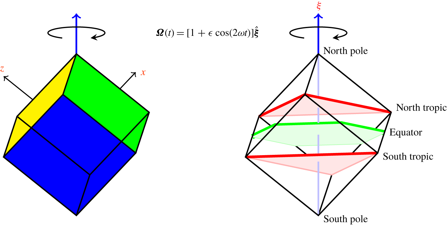
where the non-dimensional libration frequency  $2\unicode[STIX]{x1D714}=\unicode[STIX]{x1D70E}/\unicode[STIX]{x1D6FA}>0$. Figure 1 shows a schematic of the system. The non-inertial frame of reference attached to the librating cube introduces both Coriolis and Euler body forces into the (non-dimensional) governing equations:
 $$\begin{eqnarray}\frac{\unicode[STIX]{x2202}\boldsymbol{u}}{\unicode[STIX]{x2202}t}+(\boldsymbol{u}\boldsymbol{\cdot }\unicode[STIX]{x1D735})\boldsymbol{u}+2\unicode[STIX]{x1D734}\times \boldsymbol{u}+\frac{\text{d}\unicode[STIX]{x1D734}}{\text{d}t}\times \boldsymbol{x}=-\unicode[STIX]{x1D735}p+\text{E}\unicode[STIX]{x1D6FB}^{2}\boldsymbol{u},\quad \unicode[STIX]{x1D735}\boldsymbol{\cdot }\boldsymbol{u}=0,\end{eqnarray}$$
where  $p$ is the generalized pressure and
 $\text{E}=\unicode[STIX]{x1D708}/\unicode[STIX]{x1D6FA}L^{2}$ is the Ekman number. In this frame of reference, the no-slip boundary conditions are
 $\boldsymbol{u}=\mathbf{0}$ on all six walls of the cube.
Schematic of the librating cube, and the rotation axis vector  $\widehat{\unicode[STIX]{x1D743}}=(1,1,1)/\sqrt{3}$.

The vector  $\widehat{\unicode[STIX]{x1D743}}$ defines an axial coordinate
 $\unicode[STIX]{x1D709}=\widehat{\unicode[STIX]{x1D743}}\boldsymbol{\cdot }\boldsymbol{x}=(x+y+z)/\sqrt{3}$ in the direction of the rotation vector
 $\unicode[STIX]{x1D734}$. We call the plane
 $\unicode[STIX]{x1D709}=0$ the equator, containing the origin
 $(0,0,0)$. The planes
 $\unicode[STIX]{x1D709}=\pm 1/(2\sqrt{3})$, containing the vertices
 $(\mp 0.5,\pm 0.5,\pm 0.5)$,
 $(\pm 0.5,\mp 0.5,\pm 0.5)$ and
 $(\pm 0.5,\pm 0.5,\mp 0.5)$, are respectively called the north and south tropics. The vertices
 $(\pm 0.5,\pm 0.5,\pm 0.5)$ corresponding to
 $\unicode[STIX]{x1D709}=\pm \sqrt{3}/2$ are the north and south poles. The equator intersects the cube along a regular hexagon, while the north and south tropics intersect the cube along equilateral triangles. The tropical planes partition the cube into three regions: the north and south polar regions, and the tropical region between the tropics. The edges of the cube which intersect the equatorial plane are completely contained in the tropical region and are referred to as tropical edges, whereas edges connecting to the poles are contained in the polar regions and are referred to as polar edges. The angle between
 $\widehat{\unicode[STIX]{x1D743}}$ and each face of the cube is
 $\arccos (\sqrt{2/3})\approx \arccos (0.82)\approx 35^{\circ }$, while the angle between
 $\widehat{\unicode[STIX]{x1D743}}$ and each edge of the cube is
 $\arccos (\sqrt{1/3})\approx \arccos (0.58)\approx 55^{\circ }$. These angles play a critical role in the response to librational forcing, as will be detailed below.
The governing equations and boundary conditions are invariant to a discrete rotation  ${\mathcal{R}}$ of angle
 $2\unicode[STIX]{x03C0}/3$ about the rotation axis
 $\widehat{\unicode[STIX]{x1D743}}$ and a reflection through the origin
 ${\mathcal{C}}$. The actions of these two symmetries on the velocity are
 $$\begin{eqnarray}\displaystyle & \displaystyle {\mathcal{R}}:[u,v,w](x,y,z,t)\mapsto [w,u,v](z,x,y,t), & \displaystyle\end{eqnarray}$$
 $$\begin{eqnarray}\displaystyle & \displaystyle {\mathcal{C}}:[u,v,w](x,y,z,t)\mapsto [-u,-v,-w](-x,-y,-z,t). & \displaystyle\end{eqnarray}$$
The centrosymmetry  ${\mathcal{C}}$ generates a cyclic group
 $Z_{2}$ consisting of
 $\{{\mathcal{I}},{\mathcal{C}}\}$, and the rotation
 ${\mathcal{R}}$ generates a cyclic group
 $Z_{3}$ consisting of
 $\{{\mathcal{I}},{\mathcal{R}},{\mathcal{R}}^{2}\}$, where
 ${\mathcal{I}}$ is the identity, and
 ${\mathcal{C}}^{2}={\mathcal{R}}^{3}={\mathcal{I}}$. Since
 ${\mathcal{C}}{\mathcal{R}}={\mathcal{R}}{\mathcal{C}}$, the symmetry group of the system is
 $Z_{2}\times Z_{3}$. As the system is periodically forced with period
 $\unicode[STIX]{x1D70F}=\unicode[STIX]{x03C0}/\unicode[STIX]{x1D714}$, it is invariant to the time translation symmetry
 $$\begin{eqnarray}{\mathcal{T}}:[u,v,w](x,y,z,t)\mapsto [u,v,w](x,y,z,t+\unicode[STIX]{x1D70F}).\end{eqnarray}$$
The governing equations are solved via a pseudospectral method using Chebyshev polynomials of the first kind with degree less than or equal to  $n_{c}$ in each of the three directions, associated with the Chebyshev–Gauss–Lobatto collocation grid. The code is exactly the same as that used in Wu et al. (Reference Wu, Welfert and Lopez2018) and Wu, Welfert & Lopez (Reference Wu, Welfert and Lopez2020), the only difference being the details of the body force.
In order to study the flow response to librational forcing in the regime of fast mean rotation and small forcing amplitude, the Ekman number  $\text{E}$ and forcing amplitude
 $\unicode[STIX]{x1D716}$ should be as small as is practicable. To put this into perspective, experiments on a librating cube typically have
 $\text{E}\sim 10^{-5}$ and
 $\unicode[STIX]{x1D716}\sim 10^{-2}$ (Boisson et al. Reference Boisson, Lamriben, Maas, Cortet and Moisy2012), and in the related numerical study, Wu et al. (Reference Wu, Welfert and Lopez2018) used
 $\text{E}=\unicode[STIX]{x1D716}=10^{-6}$. For the present study, we have been able to push these down to
 $\text{E}=\unicode[STIX]{x1D716}=10^{-7}$, and we consider variations in the half-frequency
 $\unicode[STIX]{x1D714}\in (0,1)$. The spatial resolution used is
 $n_{c}=168$. The number of time steps used per libration period depends on
 $\unicode[STIX]{x1D714}$, and varies from 6400 for the smallest
 $\unicode[STIX]{x1D714}$ to 100 for the largest.
3 Response to low-amplitude libration
3.1 Enstrophy on the faces of the cube
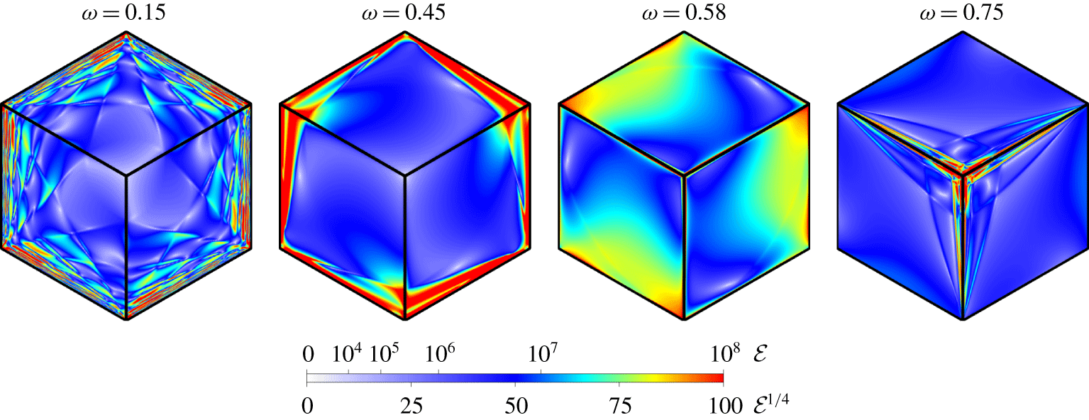
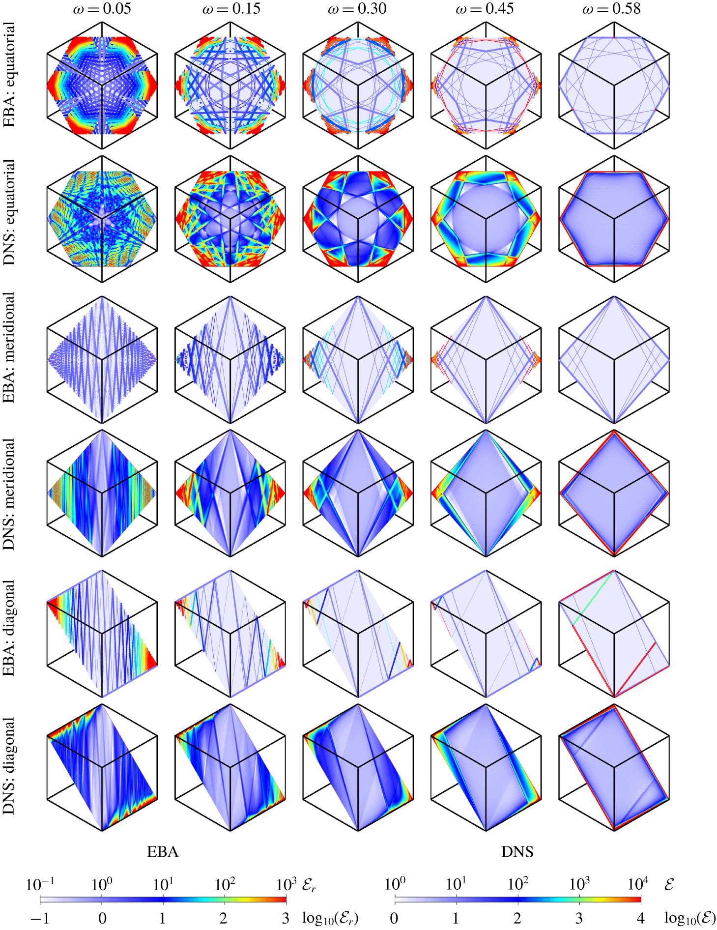
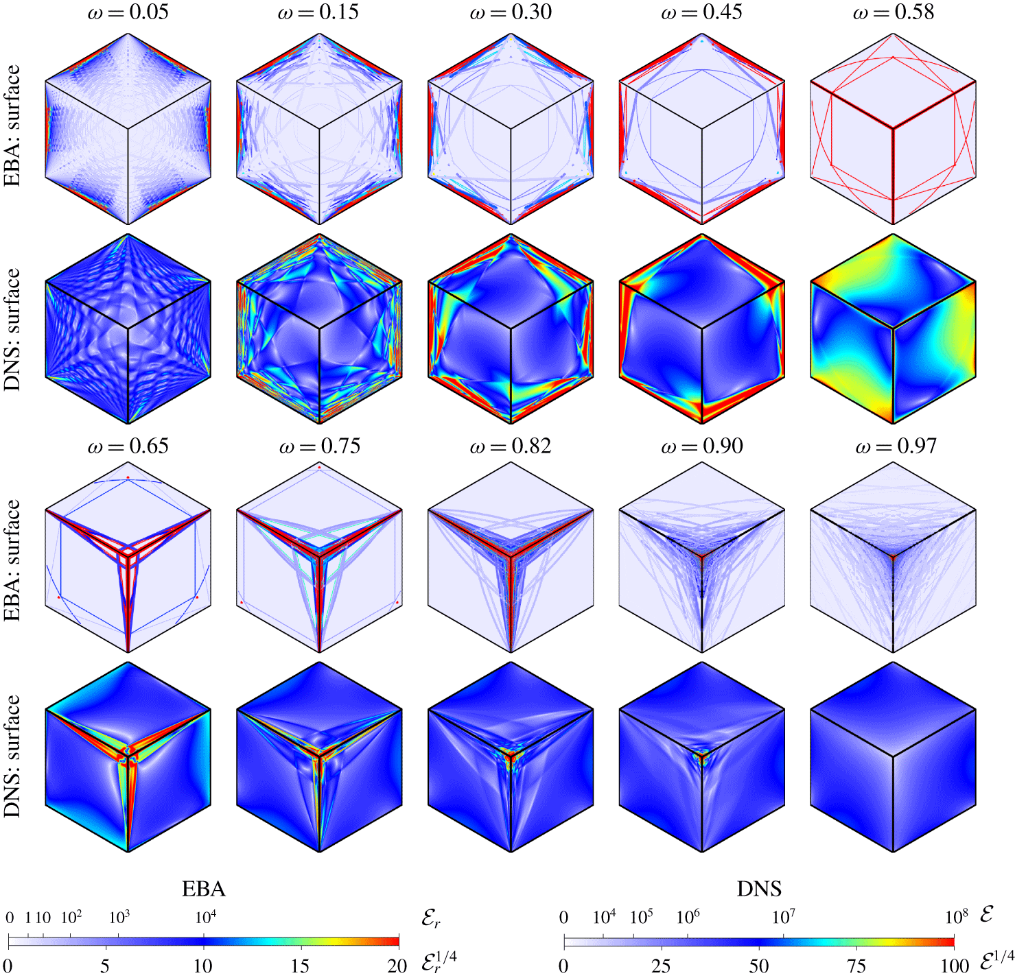
We begin by considering the enstrophy,  ${\mathcal{E}}=|\unicode[STIX]{x1D735}\times \boldsymbol{u}|^{2}$, on the faces of the cube. At the parameters considered, the enstrophy of the response flow is the same on all faces of the cube, modulo a rotation and/or a reflection, as a consequence of the invariance to the symmetries
 ${\mathcal{R}}$ and
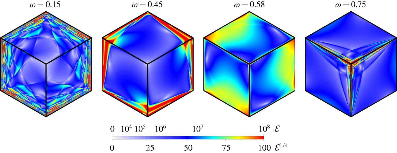
 ${\mathcal{C}}$ in the response flow. Figure 2 shows snapshots of the enstrophy on the faces of the cube at phase
 $0$ of the librational forcing for select values of
 $\unicode[STIX]{x1D714}$. The view is from above the north pole, with the rotation vector
 $\widehat{\unicode[STIX]{x1D743}}$ pointing out of the page. The six vertices surrounding the north pole are the six tropical vertices; these are connected to each other by tropical edges. Three vertices are connected to the north pole by the polar edges that are visible. The three other tropical vertices are connected to the south pole and are not visible in this view. All plots use the same colour map, with the enstrophy ranging from
 ${\mathcal{E}}=0$ (white) to
 ${\mathcal{E}}=10^{8}$ (red), and intermediate values represented by colours of the rainbow. Enstrophies larger than
 $10^{8}$ (typically up to
 $10^{10}$ around the edges) are cropped to
 $10^{8}$ to emphasize the details on the faces of the cube.
Snapshots of the enstrophy  ${\mathcal{E}}$ on the cube faces at phase
 $0$ of the forcing at half-frequencies
 $\unicode[STIX]{x1D714}$ as indicated. The colour map ranges from
 ${\mathcal{E}}=0$ (white) to
 ${\mathcal{E}}=10^{8}$ (red). The view is from a point far above the north pole; the rotation vector
 $\widehat{\unicode[STIX]{x1D743}}$ is pointing out of the page. The right half of movie 1, labelled DNS, animates snapshots of the surface enstrophy at the same phase over the half-frequency range
 $0.01\leqslant \unicode[STIX]{x1D714}\leqslant 0.99$ with
 $0.01$ increments in
 $\unicode[STIX]{x1D714}$. The bottom row of movie 2, labelled surface, animates the surface enstrophy over one libration period for several values of
 $\unicode[STIX]{x1D714}$.
The right half of movie 1 (available at https://doi.org/10.1017/jfm.2020.328), labelled DNS, consists of individual frames of the same view of the surface enstrophy at phase  $0$, with each frame corresponding to
 $\unicode[STIX]{x1D714}\in [0.01,0.99]$, with increments of 0.01, illustrating the continuous variation in the surface enstrophy with
 $\unicode[STIX]{x1D714}$. Three different regimes emerge for
 $\unicode[STIX]{x1D714}\in (0,1)$. For
 $\unicode[STIX]{x1D714}\lesssim 0.58$ (
 $\unicode[STIX]{x1D714}^{2}\lesssim 1/3$), the surface enstrophy concentrates on the tropical edges, with a criss-crossing pattern at small
 $\unicode[STIX]{x1D714}$. In contrast, for
 $\unicode[STIX]{x1D714}\gtrsim 0.58$ (
 $\unicode[STIX]{x1D714}^{2}\gtrsim 1/3$), the surface enstrophy concentrates on the polar edges, and gradually towards the poles with increasing
 $\unicode[STIX]{x1D714}$. For
 $\unicode[STIX]{x1D714}\gtrsim 0.82$ (
 $\unicode[STIX]{x1D714}^{2}\gtrsim 2/3$) the surface enstrophy is focused at the poles. At both
 $\unicode[STIX]{x1D714}\simeq 0$ and
 $\unicode[STIX]{x1D714}\simeq 1$, the surface enstrophy is significantly smaller. The bottom row of movie 2, labelled surface, animates the surface enstrophy over one libration period for several values of
 $\unicode[STIX]{x1D714}$. The sharp criss-cross patterns are seen to stay in place, periodically modulated in magnitude. In the vast regions devoid of these lines, there is a lower-energy wave that travels around the tropics in the prograde direction. This is reminiscent of the so-called whispering-gallery mode (Drijfhout & Maas Reference Drijfhout and Maas2007; Rabitti & Maas Reference Rabitti and Maas2014).
The surface enstrophy just described shows that the flow near the faces of the cube has complex spatio-temporal dynamics. The surface enstrophy has contributions from both the viscous torque (via the no-slip boundary conditions) and the pressure torque resulting from the libration (modulated rotation) of the cube, with the motion of faces having a non-trivial normal component.
3.2 Enstrophy inside the cube
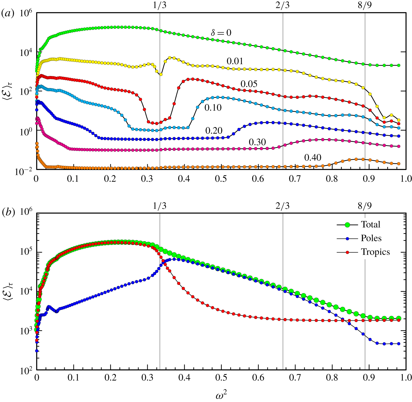
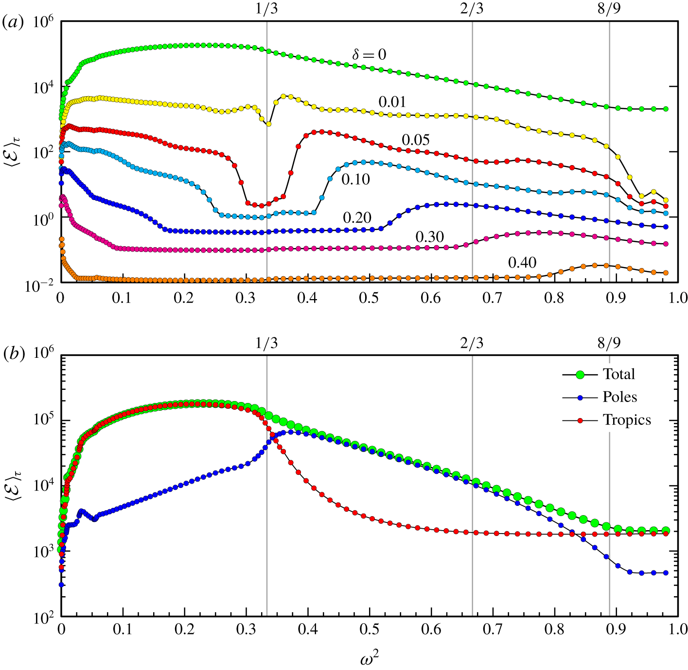
Time-averaged enstrophy response  $\langle {\mathcal{E}}\rangle _{\unicode[STIX]{x1D70F}}$ versus
 $\unicode[STIX]{x1D714}^{2}$ evaluated over
 $(a)$ the volume
 $-0.5+\unicode[STIX]{x1D6FF}\leqslant x,y,z\leqslant 0.5-\unicode[STIX]{x1D6FF}$ for
 $\unicode[STIX]{x1D6FF}$ as indicated, and
 $(b)$ the total contribution (
 $\unicode[STIX]{x1D6FF}=0$) divided up into the contributions from the polar regions and the tropics, all for
 $\text{E}=10^{-7}$ and
 $\unicode[STIX]{x1D716}=10^{-7}$.
We now examine the enstrophy of the forced flow inside the cube using the time-averaged enstrophy in subvolumes of the cube as a broad measure,
 $$\begin{eqnarray}\langle {\mathcal{E}}\rangle _{\unicode[STIX]{x1D70F}}=\frac{1}{\unicode[STIX]{x1D70F}}\int _{0}^{\unicode[STIX]{x1D70F}}\int _{-0.5+\unicode[STIX]{x1D6FF}}^{\,\,0.5-\unicode[STIX]{x1D6FF}}\int _{-0.5+\unicode[STIX]{x1D6FF}}^{\,\,0.5-\unicode[STIX]{x1D6FF}}\int _{-0.5+\unicode[STIX]{x1D6FF}}^{\,\,0.5-\unicode[STIX]{x1D6FF}}|\unicode[STIX]{x1D735}\times \boldsymbol{u}|^{2}\,\text{d}x\,\text{d}y\,\text{d}z\,\text{d}t,\end{eqnarray}$$
where  $\unicode[STIX]{x1D70F}=\unicode[STIX]{x03C0}/\unicode[STIX]{x1D714}$ is the libration period. The volume integral is over
 $-0.5+\unicode[STIX]{x1D6FF}\leqslant x,y,z\leqslant 0.5-\unicode[STIX]{x1D6FF}$, corresponding to shaving a slice of thickness
 $0\leqslant \unicode[STIX]{x1D6FF}<0.5$ from each face of the cube. Figure 3(a) shows
 $\langle {\mathcal{E}}\rangle _{\unicode[STIX]{x1D70F}}$ for various
 $\unicode[STIX]{x1D6FF}$, and quantifies how the enstrophy distribution in the cube changes with
 $\unicode[STIX]{x1D714}^{2}$. One striking aspect is that, over the entire
 $\unicode[STIX]{x1D714}^{2}$ range, a thin boundary layer region (
 $\unicode[STIX]{x1D6FF}=0.01$) contains most of the enstrophy. Figure 3(a) also shows that there is a dramatic decrease in the internal enstrophy at
 $\unicode[STIX]{x1D714}^{2}\sim 1/3$ (
 $\unicode[STIX]{x1D714}\sim 0.58$) for
 $\unicode[STIX]{x1D6FF}>0.01$. This is precisely the value of
 $\unicode[STIX]{x1D714}$ at which the surface enstrophy switches from being concentrated on the tropical edges to being concentrated on the polar edges. The total enstrophy gradually decreases as
 $\unicode[STIX]{x1D714}^{2}$ increases, before levelling off at
 $\unicode[STIX]{x1D714}^{2}\sim 8/9$ (
 $\unicode[STIX]{x1D714}\sim 0.94$), with another drop in internal enstrophy as
 $\unicode[STIX]{x1D714}\rightarrow 1$.
Figure 3(b) also shows the mean enstrophy in the entire volume ( $\unicode[STIX]{x1D6FF}=0$; green symbols), together with the contributions from the two polar regions only (
 $-1.5/\sqrt{3}\leqslant \unicode[STIX]{x1D709}\leqslant -0.5/\sqrt{3}$ and
 $0.5/\sqrt{3}\leqslant \unicode[STIX]{x1D709}\leqslant 1.5/\sqrt{3}$; blue symbols) and the tropical region only (
 $-0.5/\sqrt{3}\leqslant \unicode[STIX]{x1D709}\leqslant 0.5/\sqrt{3}$; red symbols). This very clearly shows that for
 $\unicode[STIX]{x1D714}^{2}\lesssim 1/3$ (
 $\unicode[STIX]{x1D714}\lesssim 0.58$) the total mean enstrophy resides almost exclusively in the tropics, while for
 $1/3\lesssim \unicode[STIX]{x1D714}^{2}\lesssim 2/3$ (
 $0.58\lesssim \unicode[STIX]{x1D714}\lesssim 0.82$) it is almost exclusively in the polar regions. For
 $\unicode[STIX]{x1D714}^{2}\gtrsim 2/3$ (
 $\unicode[STIX]{x1D714}\gtrsim 0.82$), there is a gradual switch back to the enstrophy being concentrated in the tropics, albeit at levels much lower than at lower
 $\unicode[STIX]{x1D714}$.
The two values of the half-frequency  $\unicode[STIX]{x1D714}=\sqrt{1/3}\approx 0.58$ and
 $\unicode[STIX]{x1D714}=\sqrt{2/3}\approx 0.82$ are related to the angles between the rotation axis
 $\widehat{\unicode[STIX]{x1D743}}$ and the edges of the cube, and between
 $\widehat{\unicode[STIX]{x1D743}}$ and the faces of the cube, respectively. Both the criss-cross enstrophy pattern on the surface of the cube at lower
 $\unicode[STIX]{x1D714}$ and the apparent connection to geometric features of the cube suggest that inertial wavebeams play an important role in organizing the distribution of enstrophy in the cube. In the following section, we first consider general theoretical aspects of these wavebeams and then specifics of these for the cube rotating about the diagonal axis
 $\widehat{\unicode[STIX]{x1D743}}$.
4 Theoretical considerations of wavebeam generation and reflections
Wavebeams in many rotating flows have been observed to emerge from edges where different types of boundary layers meet. For example, in the librating cone experiments of Greenspan (Reference Greenspan1969) and Beardsley (Reference Beardsley1970), beams were emitted from the edge where the top endwall orthogonal to the rotation axis meets the conical surface; in the simulations of Lopez & Marques (Reference Lopez and Marques2014) the beams were emitted from the edges where the axially oscillating sidewall of the rotating cylinder meets the two endwalls. Other recent observations of beams being emitted from edges between rotating and fixed/differentially rotating/librating surfaces include the experiments of Klein et al. (Reference Klein, Seelig, Kurgansky, Ghasemi, Borcia, Will, Schaller, Egbers and Harlander2014) in an annular frustum and the numerical simulations of differentially rotating split-cylinder flows of Lopez & Gutierrez-Castillo (Reference Lopez and Gutierrez-Castillo2016) and Gutierrez-Castillo & Lopez (Reference Gutierrez-Castillo and Lopez2017). Planar beams in a cube librating about the  $z$ direction were also observed experimentally (Boisson et al. Reference Boisson, Lamriben, Maas, Cortet and Moisy2012) and in simulations (Wu et al. Reference Wu, Welfert and Lopez2018). In the studies of the librating cube, as well as in the cube precessing about the
 $z$ direction (Wu et al. Reference Wu, Welfert and Lopez2020), the response flows consist of resonantly driven regular low-order modes at specific frequencies, together with planar edgebeams which exist and vary continuously with the forcing frequency. In both configurations, the edgebeams were observed to emit only from the edges where the faces of the cube that are orthogonal to the rotation axis (
 $\widehat{\boldsymbol{z}}$) meet the faces that are parallel to
 $\widehat{\boldsymbol{z}}$. As we shall demonstrate below, in the current configuration with the rotation axis aligned with a main diagonal through opposite vertices, designated as the north and south poles, edgebeams are emitted from all edges as well as vertices, with different sets of edges and vertices emitting inside the cube depending on the forcing frequency.
4.1 How inertial wavebeams are generated in the cube
As  $\text{E}\rightarrow 0$, viscous boundary layers concentrate into thin films on the faces of the librating cube and their strength, as measured by the local enstrophy, is magnified. Inertial wavebeams generated by the interactions between boundary layers at contiguous faces are emitted at edges and vertices. Once emitted, these beams are well described by polarized monochromatic waves with velocity
 $$\begin{eqnarray}\boldsymbol{u}=\boldsymbol{a}\sin \unicode[STIX]{x1D711}+\boldsymbol{b}\cos \unicode[STIX]{x1D711},\end{eqnarray}$$
where  $\unicode[STIX]{x1D711}=\boldsymbol{k}\boldsymbol{\cdot }\boldsymbol{x}-2\unicode[STIX]{x1D714}t$,
 $\boldsymbol{b}=\pm \boldsymbol{a}\times \widehat{\boldsymbol{k}}$ and
 $\widehat{\boldsymbol{k}}$ is the normalized wavevector. The
 $\pm$ sign characterizes the handedness of the wave. If
 $\boldsymbol{a}$ is orthogonal to the wavevector,
 $\boldsymbol{a}\boldsymbol{\cdot }\boldsymbol{k}=0$ (the wave is transverse), and if the dispersion relation
 $$\begin{eqnarray}(\widehat{\unicode[STIX]{x1D743}}\boldsymbol{\cdot }\widehat{\boldsymbol{k}})^{2}=\unicode[STIX]{x1D714}^{2}\end{eqnarray}$$
holds, then the wave  $\boldsymbol{u}$ and the associated pressure field
 $p=\pm 2(\widehat{\unicode[STIX]{x1D743}}\boldsymbol{\cdot }\boldsymbol{u})/|\boldsymbol{k}|$ solve the unforced inviscid equations
 $$\begin{eqnarray}\unicode[STIX]{x2202}\boldsymbol{u}/\unicode[STIX]{x2202}t+(\boldsymbol{u}\boldsymbol{\cdot }\unicode[STIX]{x1D735})\boldsymbol{u}+2\widehat{\unicode[STIX]{x1D743}}\times \boldsymbol{u}=-\unicode[STIX]{x1D735}p,\quad \unicode[STIX]{x1D735}\boldsymbol{\cdot }\boldsymbol{u}=0\end{eqnarray}$$
(see appendix A for details). The dispersion relation (4.2) defines a double cone of directions for the unit wavevector  $\widehat{\boldsymbol{k}}$ at a given half-frequency
 $\unicode[STIX]{x1D714}$. The beam’s energy propagates in the direction of the group velocity,
 $$\begin{eqnarray}\boldsymbol{c}_{g}=\unicode[STIX]{x1D735}_{\boldsymbol{k}}(2\unicode[STIX]{x1D714})=\pm 2\widehat{\unicode[STIX]{x1D743}}_{\bot }/|\boldsymbol{k}|,\end{eqnarray}$$
where  $\widehat{\unicode[STIX]{x1D743}}_{\bot }=\widehat{\unicode[STIX]{x1D743}}-(\widehat{\unicode[STIX]{x1D743}}\boldsymbol{\cdot }\widehat{\boldsymbol{k}})\widehat{\boldsymbol{k}}$ is the component of
 $\widehat{\unicode[STIX]{x1D743}}$ orthogonal to
 $\widehat{\boldsymbol{k}}$, with
 $|\widehat{\unicode[STIX]{x1D743}}_{\bot }|=(1-\unicode[STIX]{x1D714}^{2})^{1/2}$. This group velocity satisfies the transversality condition
 $\boldsymbol{c}_{g}\boldsymbol{\cdot }\widehat{\boldsymbol{k}}=0$, so that, without loss of generality,
 $$\begin{eqnarray}\widehat{\boldsymbol{a}}=\pm (1-\unicode[STIX]{x1D714}^{2})^{-1/2}\,\widehat{\unicode[STIX]{x1D743}}_{\bot }.\end{eqnarray}$$
The relation
 $$\begin{eqnarray}(\widehat{\unicode[STIX]{x1D743}}\boldsymbol{\cdot }\widehat{\boldsymbol{a}})^{2}=1-\unicode[STIX]{x1D714}^{2}\end{eqnarray}$$
defines a double cone of directions for  $\widehat{\boldsymbol{a}}$, which is dual to the cone containing
 $\widehat{\boldsymbol{k}}$, in the sense that the apertures of the two double cones are complementary.
4.1.1 Planar edgebeams
In general, points on the same edge emit beams in parallel directions that vary continuously along the edge. For the straight edges of the cube, these beams form planar sheets. The continuum of beams making up the sheet have the same  $\widehat{\boldsymbol{a}}$, but possibly different magnitudes
 $|\boldsymbol{a}|$. These magnitudes cannot be determined from inviscid considerations. In the inviscid limit
 $\text{E}\rightarrow 0$, the orientation
 $\widehat{\boldsymbol{a}}$ of an emitted wavebeam on the dual cone and the resulting orientation of the planar sheet are determined by enforcing space-time symmetries of the unforced inviscid equations (4.3) for the cube rotating about
 $\widehat{\unicode[STIX]{x1D743}}$. These symmetries result from composing the symmetries
 ${\mathcal{C}}$ or
 ${\mathcal{R}}$ with the time-reversal symmetry
 ${\mathcal{S}}$, whose action on the velocity is
 $$\begin{eqnarray}{\mathcal{S}}:[u,v,w](x,y,z,t)\mapsto [-u,-w,-v](x,z,y,-t).\end{eqnarray}$$
Note that  ${\mathcal{S}}$ is a symmetry of the inviscid system (4.3), but not of the Navier–Stokes system (2.2). For an edge in the planes
 $x=\pm 0.5$,
 ${\mathcal{S}}$ reverses the phase
 $\unicode[STIX]{x1D711}$ (with appropriate modification of the wavevector
 $\boldsymbol{k}$) and constraints the
 $y$ and
 $z$ components of
 $\boldsymbol{a}$ to be equal. As a result,
 $\widehat{\boldsymbol{a}}$ must point in the direction of a vector
 $(\unicode[STIX]{x1D6FD},1,1)$, where
 $\unicode[STIX]{x1D6FD}$ is a root of the quadratic equation obtained from (4.6),
 $$\begin{eqnarray}(\unicode[STIX]{x1D6FD}+2)^{2}=3(1-\unicode[STIX]{x1D714}^{2})(\unicode[STIX]{x1D6FD}^{2}+2).\end{eqnarray}$$
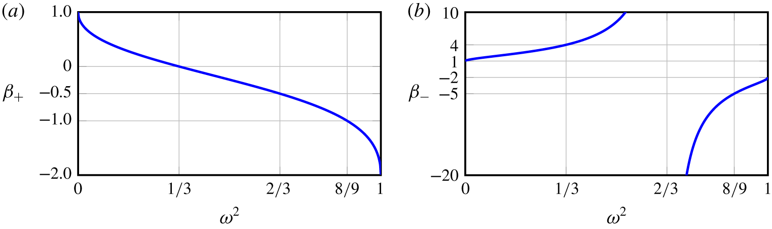
The two roots of (4.8),
 $$\begin{eqnarray}\unicode[STIX]{x1D6FD}_{\pm }=\frac{1-3\unicode[STIX]{x1D714}^{2}}{1\pm 3\sqrt{\unicode[STIX]{x1D714}^{2}(1-\unicode[STIX]{x1D714}^{2})/2}},\end{eqnarray}$$
correspond to two rays with directions  $\boldsymbol{a}_{\pm }\propto (\unicode[STIX]{x1D6FD}_{\pm },1,1)$, which are the intersections of the primary double cone, whose apex is at a point
 $p_{0}$ on the edge, with the plane containing
 $p_{0}$ and parallel to the symmetry plane
 $y=z$, forming what is commonly known as a St. Andrew’s cross. The values
 $\unicode[STIX]{x1D6FD}_{\pm }$ determine the directions
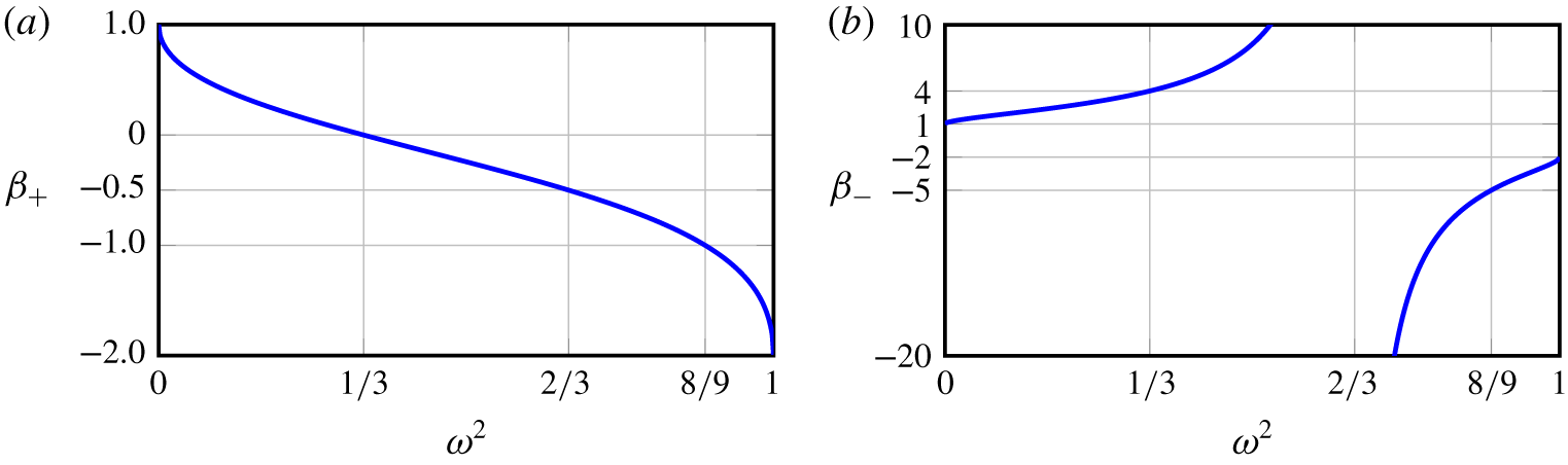
 $(\unicode[STIX]{x1D6FD}_{\pm },1,1)$ of the waves emitted from the edge, and are plotted in figure 4 as functions of
 $\unicode[STIX]{x1D714}^{2}\in (0,1)$. Figure 4 identifies four
 $\unicode[STIX]{x1D714}^{2}$ regimes where qualitatively different behaviours of the beams are found.
Functions  $\unicode[STIX]{x1D6FD}_{\pm }(\unicode[STIX]{x1D714}^{2})$ from (4.9), determining the group velocity directions of the emitted waves.
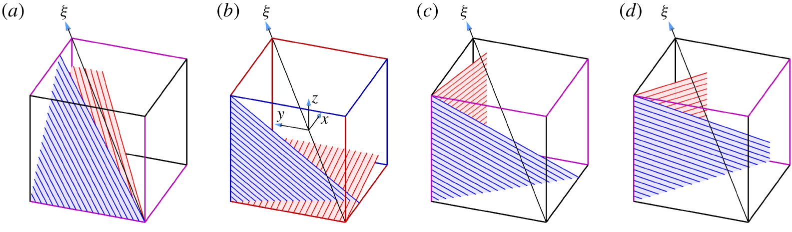
Two edgebeams formed by parallel wavebeams emitted from the polar edge  $x=z=-0.5$ and/or the tropical edge
 $x=-y=-0.5$, depending on
 $\unicode[STIX]{x1D714}^{2}$: (a)
 $\unicode[STIX]{x1D714}^{2}<1/3$ (
 $\unicode[STIX]{x1D714}=0.15$ is shown); (b)
 $1/3<\unicode[STIX]{x1D714}^{2}<2/3$ (
 $\unicode[STIX]{x1D714}=0.75$ is shown); (c)
 $2/3<\unicode[STIX]{x1D714}^{2}<8/9$ (
 $\unicode[STIX]{x1D714}=0.90$ is shown); and (d)
 $\unicode[STIX]{x1D714}^{2}>8/9$ (
 $\unicode[STIX]{x1D714}=0.98$ is shown). Like-coloured edges emit similar edgebeams related by the symmetries
 ${\mathcal{C}}$ and
 ${\mathcal{S}}$.
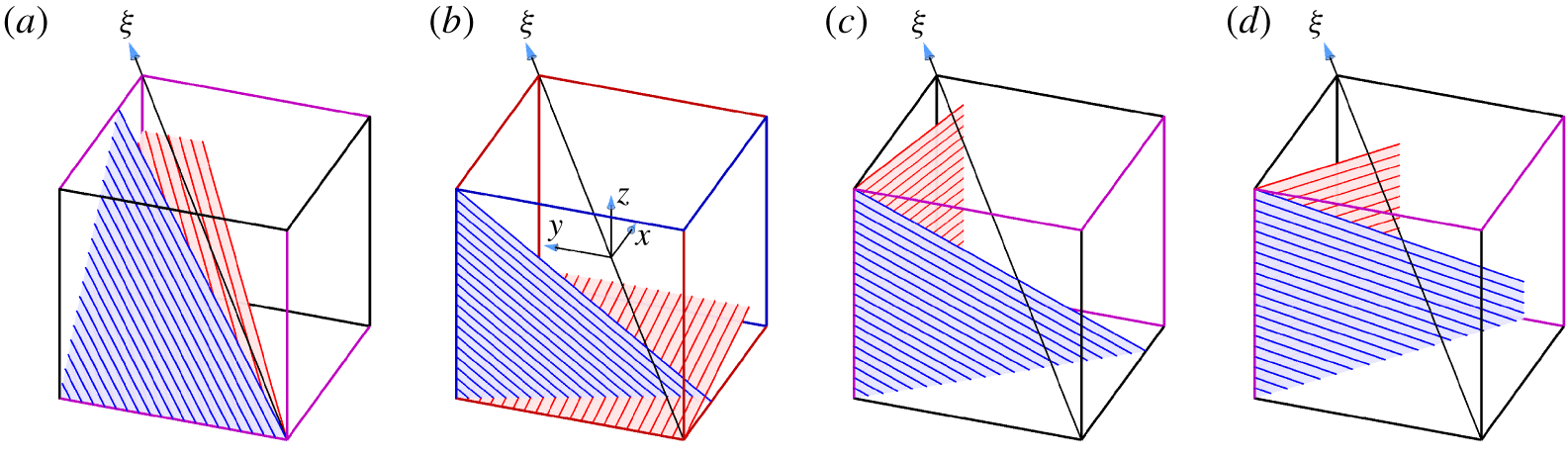
Figure 5 shows examples of wavebeams emitted from the polar edge at  $x=z=-0.5$ and the tropical edge at
 $x=-y=-0.5$ in the different
 $\unicode[STIX]{x1D714}^{2}$ regimes.
For  $\unicode[STIX]{x1D714}^{2}<1/3$, both
 $\unicode[STIX]{x1D6FD}_{\pm }>0$, and so the polar edge emits two edgebeams in directions
 $\boldsymbol{a}_{\pm }$, which are both inwards. These edgebeams are illustrated in figure 5(a). The tropical edge does not emit any wavebeam inside the cube because the dual double cone with apex on this edge is entirely outside the cube. The other five polar edges, which are like-coloured (magenta) in figure 5(a), emit similar edgebeams that are related via the symmetries
 ${\mathcal{C}}$ and
 ${\mathcal{R}}$, for a total of 12 edgebeams, two emitted from each of the six polar edges. Some of these edgebeams intersect each other.
For  $1/3<\unicode[STIX]{x1D714}^{2}<2/3$,
 $\unicode[STIX]{x1D6FD}_{+}<0<\unicode[STIX]{x1D6FD}_{-}$, so that
 $\boldsymbol{a}_{-}$ is inwards while
 $\boldsymbol{a}_{+}$ is outwards. The polar edge emits in the direction
 $\boldsymbol{a}_{-}$, but not in the direction
 $\boldsymbol{a}_{+}$. Instead, the tropical edge emits in the direction
 $-\boldsymbol{a}_{+}$. The two resulting edgebeams are illustrated in figure 5(b). All six polar edges emit one (red) edgebeam in a direction obtained via the symmetries
 ${\mathcal{C}}$ and
 ${\mathcal{R}}$ acting on
 $\boldsymbol{a}_{-}$, while all tropical edges emit one (blue) edgebeam in a direction obtained via
 ${\mathcal{C}}$ and
 ${\mathcal{R}}$ acting on
 $-\boldsymbol{a}_{+}$, for a total of 12 edgebeams. The respective edges are colour coded, red or blue, according to the direction,
 $-\boldsymbol{a}_{+}$ or
 $\boldsymbol{a}_{-}$, of the beam being emitted from them.
For  $\unicode[STIX]{x1D714}^{2}>2/3$, both
 $\unicode[STIX]{x1D6FD}_{\pm }<0$ and the polar edges do not emit any beam inside the cube. The tropical edge emits two edgebeams in directions
 $-\boldsymbol{a}_{\pm }$ (see figure 5c). Each of the six tropical edges emits two edgebeams obtained via the symmetries
 ${\mathcal{C}}$ and
 ${\mathcal{R}}$, for a total of 12 edgebeams. At
 $\unicode[STIX]{x1D714}^{2}=8/9$ the wavebeam emitted from the tropical vertex
 $(-0.5,0.5,0.5)$ in the direction
 $-\boldsymbol{a}_{+}$ hits the opposite tropical vertex at
 $(0.5,-0.5,-0.5)$. For
 $\unicode[STIX]{x1D714}^{2}>8/9$, this wavebeam impinges on the face of the cube at
 $x=0.5$, rather than on the polar edge at
 $y=z=-0.5$ (figure 5d). This switch is associated with the reduced enstrophy response for
 $\unicode[STIX]{x1D714}\sim 1$ observed in figure 3.
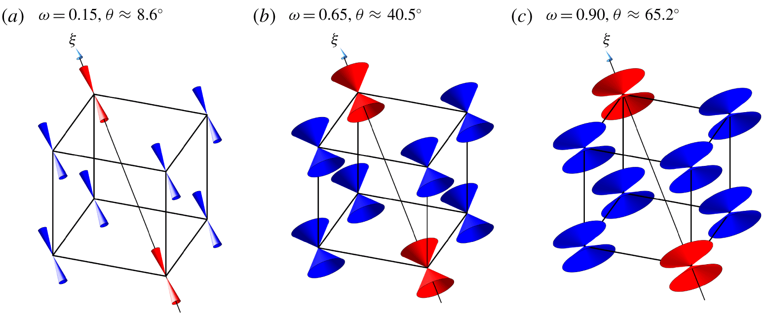
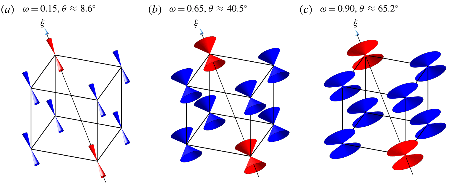
Schematics of conical vertex beams (red for beams emitted from polar vertices and blue for beams from tropical vertices), at three values of  $\unicode[STIX]{x1D714}$ representative of the three
 $\unicode[STIX]{x1D714}^{2}$ regimes.
4.1.2 Conical vertex beams
Wavebeams are also emitted from the vertices of the librating cube. The vertices are point sources, from which conical sheets of wavebeams are emitted. Depending on  $\unicode[STIX]{x1D714}$ and the vertex considered, the conical vertex beam may be emitted either completely inside, partially inside or completely outside the cube. Each vertex emits a double conical vertex beam with angle
 $\unicode[STIX]{x1D703}$ from the axis of rotation such that
 $\cos ^{2}\unicode[STIX]{x1D703}=1-\unicode[STIX]{x1D714}^{2}$. In the
 $\unicode[STIX]{x1D714}^{2}<1/3$ regime, the two poles each emit one conical beam in the direction of the opposite pole, and another conical beam away from the cube. The two conical beams emitted from each tropical vertex remain completely outside the cube. Figure 6(a) is a schematic illustrating this for
 $\unicode[STIX]{x1D714}=0.15$. The two polar conical beams are symmetrically related by
 ${\mathcal{C}}$ and intersect the equatorial plane along a circle. Intersections with other planes are conic sections (ellipses, parabolas or hyperbolas). In the
 $1/3<\unicode[STIX]{x1D714}^{2}<2/3$ regime, for the polar vertices, one of the conical beams from the double cone is completely outside the cube and the other is partially inside the cube, whereas for the tropical vertices, part of the conical beam on one side of the double cone is emitted inside the cube, as illustrated in figure 6(b). The intersections of these with planes inside the cube lead to other conic sections. In the
 $\unicode[STIX]{x1D714}^{2}>2/3$ regime, the polar beams are completely outside the cube, while the tropical conical beams from both parts of the double cone are partially inside the cube (see figure 6c).
4.2 How inertial wavebeams are reflected at the cube walls
Confinement leads to the beams that are emitted from edges impinging onto and reflecting off surfaces of the cube. The reflected beam is also circularly polarized, with velocity
 $$\begin{eqnarray}\boldsymbol{u}^{\prime }=\boldsymbol{a}^{\prime }\sin \unicode[STIX]{x1D711}^{\prime }+\boldsymbol{b}^{\prime }\cos \unicode[STIX]{x1D711}^{\prime },\end{eqnarray}$$
where  $\unicode[STIX]{x1D711}^{\prime }=\boldsymbol{k}^{\prime }\boldsymbol{\cdot }\boldsymbol{x}-2\unicode[STIX]{x1D714}^{\prime }t$ and
 $\boldsymbol{b}^{\prime }=\pm \boldsymbol{a}^{\prime }\times \widehat{\boldsymbol{k}^{\prime }}$. Phillips (Reference Phillips1963) laid down the criteria determining how waves are reflected from a surface with unit normal
 $\widehat{\boldsymbol{n}}$: (i) the reflected and incident waves,
 $\boldsymbol{u}^{\prime }$ and
 $\boldsymbol{u}$, should have the same half-frequency
 $\unicode[STIX]{x1D714}^{\prime }=\unicode[STIX]{x1D714}$, (ii) the tangential component of the associated wavevectors,
 $\boldsymbol{k}^{\prime }$ and
 $\boldsymbol{k}$, should be equal,
 $\boldsymbol{k}^{\prime }\times \widehat{\boldsymbol{n}}=\boldsymbol{k}\times \widehat{\boldsymbol{n}}$, and (iii) the reflected wave should obey the dispersion relation,
 $(\widehat{\unicode[STIX]{x1D743}}\boldsymbol{\cdot }\widehat{\boldsymbol{k}^{\prime }})^{2}=\unicode[STIX]{x1D714}^{\prime 2}$.
The condition that the tangential components be equal,  $\boldsymbol{k}^{\prime }\times \widehat{\boldsymbol{n}}=\boldsymbol{k}\times \widehat{\boldsymbol{n}}$, is equivalent to the condition that their difference is normal to the reflecting surface,
 $(\boldsymbol{k}^{\prime }-\boldsymbol{k})\Vert \widehat{\boldsymbol{n}}$. This implies a relationship of the form
 $$\begin{eqnarray}\boldsymbol{k}^{\prime }=\boldsymbol{k}-2s|\boldsymbol{k}|\widehat{\boldsymbol{n}},\end{eqnarray}$$
where  $s$ depends on the angles between the axis of rotation
 $\widehat{\unicode[STIX]{x1D743}}$, the normal to the reflecting surface
 $\widehat{\boldsymbol{n}}$ and the incident wavevector
 $\boldsymbol{k}$. From (4.11) one obtains
 $$\begin{eqnarray}|\boldsymbol{k}^{\prime }|^{2}=|\boldsymbol{k}|^{2}(1-4\unicode[STIX]{x1D70C}s+4s^{2})\quad \text{and}\quad \widehat{\unicode[STIX]{x1D743}}\boldsymbol{\cdot }\boldsymbol{k}^{\prime }=(\widehat{\unicode[STIX]{x1D743}}\boldsymbol{\cdot }\boldsymbol{k})(1-2\unicode[STIX]{x1D706}s),\end{eqnarray}$$
where
 $$\begin{eqnarray}\unicode[STIX]{x1D70C}=\widehat{\boldsymbol{k}}\boldsymbol{\cdot }\widehat{\boldsymbol{n}}\quad \text{and}\quad \unicode[STIX]{x1D706}=(\widehat{\unicode[STIX]{x1D743}}\boldsymbol{\cdot }\widehat{\boldsymbol{n}})/(\widehat{\unicode[STIX]{x1D743}}\boldsymbol{\cdot }\widehat{\boldsymbol{k}}).\end{eqnarray}$$
The scalar  $-1<\unicode[STIX]{x1D70C}<1$ is the cosine of the angle between the incident wavevector
 $\boldsymbol{k}$ and the normal
 $\widehat{\boldsymbol{n}}$ to the reflecting surface. The scalar
 $\unicode[STIX]{x1D706}$ is the ratio of cosines of the angles between the rotation axis
 $\widehat{\unicode[STIX]{x1D743}}$ and the normal
 $\widehat{\boldsymbol{n}}$ to the reflecting surface, and between the rotation axis
 $\widehat{\unicode[STIX]{x1D743}}$ and the incident wavevector
 $\boldsymbol{k}$. This ratio determines whether
 $\widehat{\boldsymbol{n}}$ is outside (subcritical reflection,
 $|\unicode[STIX]{x1D706}|<1$), on (critical reflection,
 $|\unicode[STIX]{x1D706}|=1$) or inside (supercritical reflection,
 $|\unicode[STIX]{x1D706}|>1$) the primary (double) cone containing the wavevectors
 $\boldsymbol{k}$ and
 $\boldsymbol{k}^{\prime }$. In the cube rotating about
 $\widehat{\unicode[STIX]{x1D743}}$,
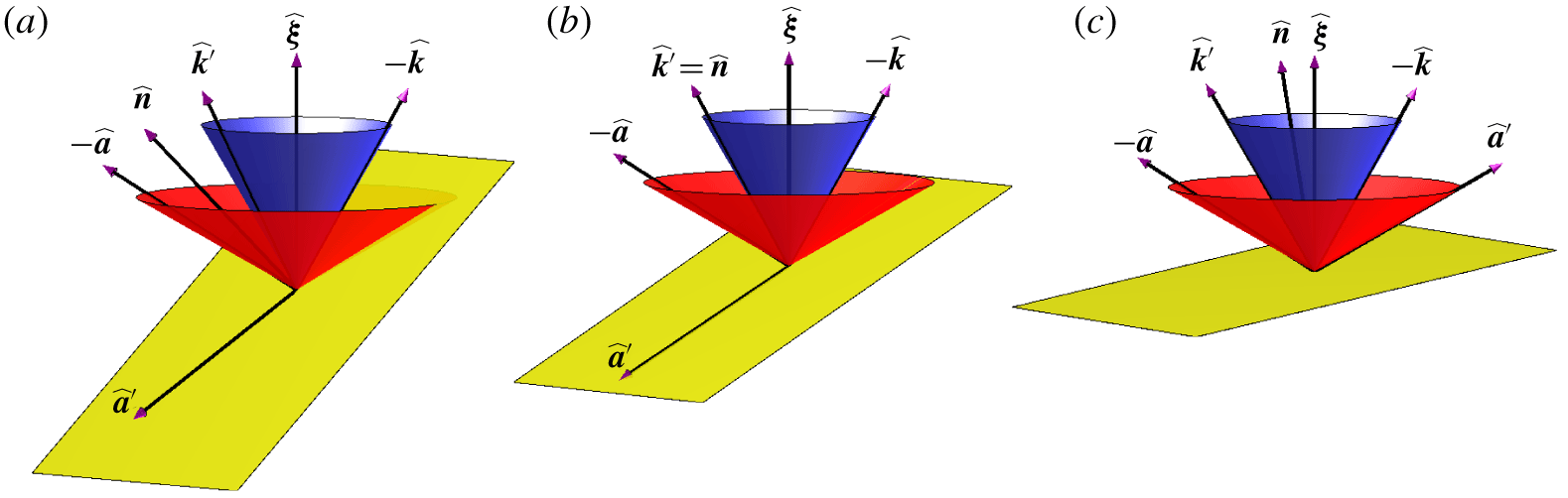
 $\unicode[STIX]{x1D706}^{2}=1/(3\unicode[STIX]{x1D714}^{2})$ for all reflections on the faces of the cube. Figure 7 shows schematics of these three cases when the primary cone is inside the dual cone. Using (4.12), the condition
 $(\widehat{\unicode[STIX]{x1D743}}\boldsymbol{\cdot }\widehat{\boldsymbol{k}^{\prime }})^{2}={\unicode[STIX]{x1D714}^{\prime }}^{2}=\unicode[STIX]{x1D714}^{2}=(\widehat{\unicode[STIX]{x1D743}}\boldsymbol{\cdot }\widehat{\boldsymbol{k}})^{2}$ yields
 $$\begin{eqnarray}1-4\unicode[STIX]{x1D70C}s+4s^{2}=|\boldsymbol{k}^{\prime }|^{2}/|\boldsymbol{k}|^{2}=(\widehat{\unicode[STIX]{x1D743}}\boldsymbol{\cdot }\boldsymbol{k}^{\prime })^{2}/(\widehat{\unicode[STIX]{x1D743}}\boldsymbol{\cdot }\boldsymbol{k})^{2}=(1-2\unicode[STIX]{x1D706}s)^{2},\end{eqnarray}$$
whose non-trivial solution is
 $$\begin{eqnarray}s=(\unicode[STIX]{x1D70C}-\unicode[STIX]{x1D706})/(1-\unicode[STIX]{x1D706}^{2}).\end{eqnarray}$$
The relation (4.11) reduces to a standard Euclidean reflection (i.e. a reflection about the normal vector  $\widehat{\boldsymbol{n}}$),
 $s=\unicode[STIX]{x1D70C}$, if
 $\unicode[STIX]{x1D706}=0$ (the rotation axis is orthogonal to the reflecting wall,
 $\widehat{\unicode[STIX]{x1D743}}\bot \widehat{\boldsymbol{n}}$) or if
 $\unicode[STIX]{x1D706}=1/\unicode[STIX]{x1D70C}$ (the wavevector
 $\boldsymbol{k}$ is orthogonal to the component of
 $\widehat{\unicode[STIX]{x1D743}}$ tangential to the reflecting wall,
 $\boldsymbol{k}\bot \widehat{\boldsymbol{n}}\times (\widehat{\unicode[STIX]{x1D743}}\times \widehat{\boldsymbol{n}})$, which holds for any
 $\boldsymbol{k}$ if the rotation axis is parallel to the reflecting wall,
 $\widehat{\unicode[STIX]{x1D743}}\,\Vert \,\widehat{\boldsymbol{n}}$).
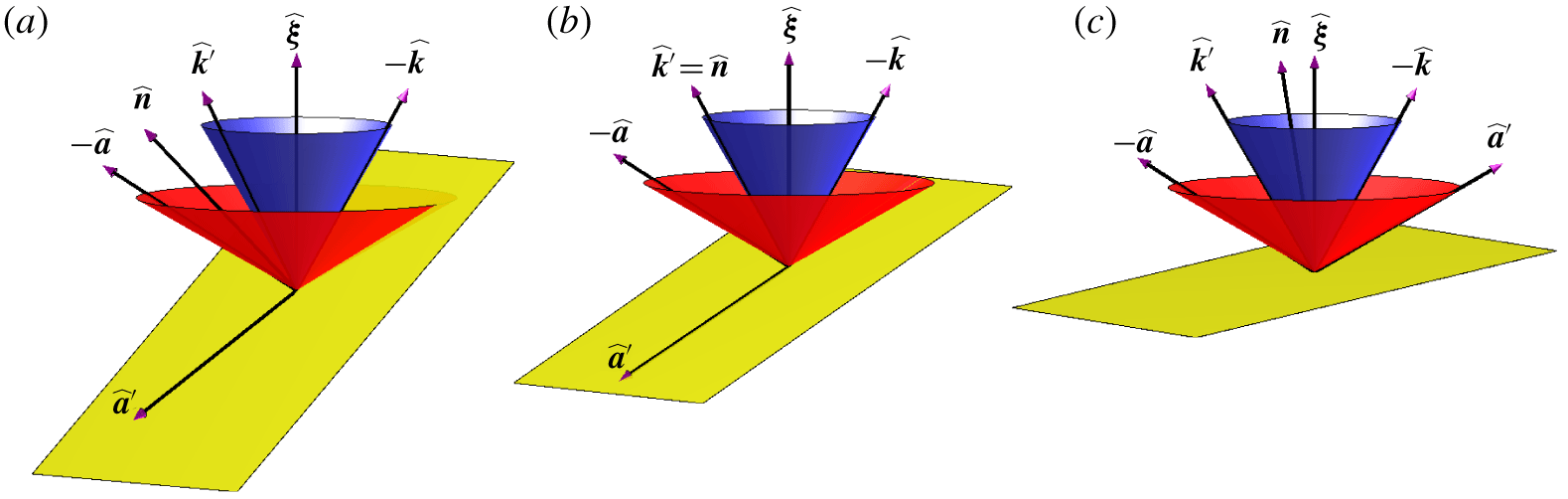
Schematics of the tangent plane (yellow) at the reflecting point in relation to the primary cone (blue) containing the incident and reflected wavevectors,  $\widehat{\boldsymbol{k}}$ and
 $\widehat{\boldsymbol{k}^{\prime }}$, and the dual cone (red) containing the incident and reflected group velocity directions
 $\widehat{\boldsymbol{a}}$ and
 $\widehat{\boldsymbol{a}^{\prime }}$, in the (a) subcritical (
 $|\unicode[STIX]{x1D706}|<1$), (b) critical (
 $|\unicode[STIX]{x1D706}|=1$) and (c) supercritical (
 $1<|\unicode[STIX]{x1D706}|\leqslant 1/\unicode[STIX]{x1D714}$) cases. The vectors
 $\widehat{\boldsymbol{k}^{\prime }}$,
 $\widehat{\boldsymbol{k}}$ and
 $\widehat{\boldsymbol{n}}$ are coplanar,
 $\widehat{\boldsymbol{k}}$ and
 $\widehat{\boldsymbol{a}}$ are orthogonal, and
 $\widehat{\boldsymbol{k}^{\prime }}$ and
 $\widehat{\boldsymbol{a}^{\prime }}$ are also orthogonal.
The formulation of (4.11) provides a simple vectorial approach to the reflection of inertial wavebeams that extends the Euclidean framework. The relation between incident and reflected waves,  $\boldsymbol{k}$ and
 $\boldsymbol{k}^{\prime }$, is usually presented in component rather than vector form, as in Manders & Maas (Reference Manders and Maas2004, equation (5a–c)), or is expressed in terms of angles
 $\unicode[STIX]{x1D713}$,
 $\unicode[STIX]{x1D703}$,
 $\unicode[STIX]{x1D6FC}$ and
 $\unicode[STIX]{x1D719}$, where
 $\cos \unicode[STIX]{x1D713}=\widehat{\unicode[STIX]{x1D743}}\boldsymbol{\cdot }\widehat{\boldsymbol{k}}$,
 $\unicode[STIX]{x1D703}=\unicode[STIX]{x03C0}/2-\unicode[STIX]{x1D713}$,
 $\sin \unicode[STIX]{x1D6FC}=\widehat{\unicode[STIX]{x1D743}}\boldsymbol{\cdot }\widehat{\boldsymbol{n}}$ and
 $\unicode[STIX]{x1D719}$ is the angle between
 $\boldsymbol{k}_{\bot }^{\phantom{\prime }}$ and
 $\widehat{\boldsymbol{n}}_{\bot }^{\phantom{\prime }}$, where
 $\boldsymbol{k}_{\bot }^{\phantom{\prime }}$ is the component of
 $\boldsymbol{k}$ orthogonal to
 $\widehat{\unicode[STIX]{x1D743}}$ and
 $\widehat{\boldsymbol{n}}_{\bot }^{\phantom{\prime }}$ is the along-slope direction. In particular, (4.11) implies that
 $\boldsymbol{k}_{\bot }^{\prime }$ satisfies a similar relation,
 $$\begin{eqnarray}\boldsymbol{k}_{\bot }^{\prime }=\boldsymbol{k}_{\bot }^{\phantom{\prime }}-2s|\boldsymbol{k}|\widehat{\boldsymbol{n}}_{\bot }^{\phantom{\prime }},\end{eqnarray}$$
so that the angle  $\unicode[STIX]{x1D719}^{\prime }$ between
 $\boldsymbol{k}_{\bot }^{\prime }$ and
 $\widehat{\boldsymbol{n}}_{\bot }^{\phantom{\prime }}$ is related to the angle
 $\unicode[STIX]{x1D719}$ between
 $\boldsymbol{k}_{\bot }^{\phantom{\prime }}$ and
 $\widehat{\boldsymbol{n}}_{\bot }^{\phantom{\prime }}$ by
 $$\begin{eqnarray}\sin \unicode[STIX]{x1D719}^{\prime }=\frac{|\boldsymbol{k}_{\bot }^{\prime }\times \widehat{\boldsymbol{n}}_{\bot }^{\phantom{\prime }}|}{|\boldsymbol{k}_{\bot }^{\prime }|\,|\widehat{\boldsymbol{n}}_{\bot }^{\phantom{\prime }}|}=\frac{|\boldsymbol{k}_{\bot }^{\phantom{\prime }}\times \widehat{\boldsymbol{n}}_{\bot }^{\phantom{\prime }}|}{|\boldsymbol{k}_{\bot }^{\prime }|\,|\widehat{\boldsymbol{n}}_{\bot }^{\phantom{\prime }}|}=\frac{|\boldsymbol{k}_{\bot }^{\phantom{\prime }}|}{|\boldsymbol{k}_{\bot }^{\prime }|}\sin \unicode[STIX]{x1D719}=\frac{|\boldsymbol{k}^{\phantom{\prime }}|}{|\boldsymbol{k}^{\prime }|}\sin \unicode[STIX]{x1D719}=\frac{\sin \unicode[STIX]{x1D719}}{|\unicode[STIX]{x1D6FC}|},\end{eqnarray}$$
as in Maas (Reference Maas2005, p. 2774), Rabitti & Maas (Reference Rabitti and Maas2013, equation (A10)) and Pillet, Maas & Dauxois (Reference Pillet, Maas and Dauxois2019, equation (2.15)), as well as Eriksen (Reference Eriksen1982, equation (8)) and Manders & Maas (Reference Manders and Maas2004, equation (7)) in equivalent forms. Upon focusing,  $|\unicode[STIX]{x1D6FC}|>1$,
 $\sin \unicode[STIX]{x1D719}^{\prime }<\sin \unicode[STIX]{x1D719}$ and the beams align themselves with the along-slope direction,
 $\widehat{\boldsymbol{n}}_{\bot }$. We find the vectorial form (4.11) to be more convenient than (4.17) for handling successive reflections, and critical in obtaining results regarding the focusing of wavebeams towards edges or vertices.
The change in wavelength upon reflection is determined by the ratio of reflected-to-incident wavevector magnitudes,
 $$\begin{eqnarray}|\unicode[STIX]{x1D6FC}|=|\boldsymbol{k}^{\prime }|/|\boldsymbol{k}|,\end{eqnarray}$$
with  $\unicode[STIX]{x1D6FC}=1-2\unicode[STIX]{x1D706}s=(1-2\unicode[STIX]{x1D70C}\unicode[STIX]{x1D706}+\unicode[STIX]{x1D706}^{2})/(1-\unicode[STIX]{x1D706}^{2})$ from (4.14) and (4.15). The ratio (4.18) agrees with both Phillips (Reference Phillips1963, equation (2.8)) and Eriksen (Reference Eriksen1982, equation (5)), and is equivalent to Manders & Maas (Reference Manders and Maas2004, equation (6)). The wavevector magnitude is conserved upon reflection,
 $|\unicode[STIX]{x1D6FC}|=1$, in the Euclidean cases
 $s=\unicode[STIX]{x1D70C}$ with
 $\unicode[STIX]{x1D706}=0$ or
 $\unicode[STIX]{x1D706}=1/\unicode[STIX]{x1D70C}$, or if
 $s=0$ with
 $\unicode[STIX]{x1D706}=\unicode[STIX]{x1D70C}$ corresponding to
 $\widehat{\boldsymbol{a}}\bot \widehat{\boldsymbol{n}}$ (group velocity tangential to the reflecting surface). An increase in wavevector magnitude,
 $|\unicode[STIX]{x1D6FC}|>1$, results in a decrease in wavelength and focusing, whereupon
 $\unicode[STIX]{x1D70C}\unicode[STIX]{x1D706}\in (\unicode[STIX]{x1D706}^{2},1)$ (subcritical case) or
 $\unicode[STIX]{x1D70C}\unicode[STIX]{x1D706}\in (1,\unicode[STIX]{x1D706}^{2})$ (supercritical case). Note that both
 $\unicode[STIX]{x1D70C}\unicode[STIX]{x1D706}=(\widehat{\boldsymbol{k}}\boldsymbol{\cdot }\widehat{\boldsymbol{n}})(\widehat{\unicode[STIX]{x1D743}}\boldsymbol{\cdot }\widehat{\boldsymbol{n}})/(\widehat{\unicode[STIX]{x1D743}}\boldsymbol{\cdot }\widehat{\boldsymbol{k}})$ and
 $\unicode[STIX]{x1D706}^{2}=(\widehat{\unicode[STIX]{x1D743}}\boldsymbol{\cdot }\widehat{\boldsymbol{n}})^{2}/(\widehat{\unicode[STIX]{x1D743}}\boldsymbol{\cdot }\widehat{\boldsymbol{k}})^{2}$ are independent of the orientation of
 $\widehat{\boldsymbol{k}}$,
 $\widehat{\boldsymbol{n}}$ or
 $\widehat{\unicode[STIX]{x1D743}}$.
The reflected beam (4.10) has group velocity
 $$\begin{eqnarray}\boldsymbol{c}_{g}^{\prime }=\unicode[STIX]{x1D735}_{\boldsymbol{ k}^{\prime }}(2\unicode[STIX]{x1D714}^{\prime })=\pm 2\widehat{\unicode[STIX]{x1D743}}_{\bot }^{\prime }/|\boldsymbol{k}^{\prime }|,\end{eqnarray}$$
where 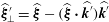 $\widehat{\unicode[STIX]{x1D743}}_{\bot }^{\prime }=\widehat{\unicode[STIX]{x1D743}}-(\widehat{\unicode[STIX]{x1D743}}\boldsymbol{\cdot }\widehat{\boldsymbol{k}^{\prime }})\widehat{\boldsymbol{k}^{\prime }}$ is the component of
 $\widehat{\unicode[STIX]{x1D743}}$ orthogonal to
 $\widehat{\boldsymbol{k}^{\prime }}$, with
 $|\widehat{\unicode[STIX]{x1D743}}_{\bot }^{\prime }|=(1-\unicode[STIX]{x1D714}^{2})^{1/2}$. Setting
 $$\begin{eqnarray}\widehat{\boldsymbol{a}^{\prime }}=\pm (1-\unicode[STIX]{x1D714}^{2})^{-1/2}\,\widehat{\unicode[STIX]{x1D743}}_{\bot }^{\prime },\end{eqnarray}$$
the no-penetration condition  $(\boldsymbol{a}+\boldsymbol{a}^{\prime })\boldsymbol{\cdot }\widehat{\boldsymbol{n}}=0$ (Phillips Reference Phillips1963) in the direction of the group velocity at the reflecting surface (
 $\widehat{\boldsymbol{n}}\boldsymbol{\cdot }\boldsymbol{x}=0$) is then satisfied if
 $$\begin{eqnarray}|\boldsymbol{a}^{\prime }|/|\boldsymbol{a}|=|\unicode[STIX]{x1D6FC}|\end{eqnarray}$$
(see appendix B for a justification). The relation  $|\boldsymbol{a}^{\prime }|/|\boldsymbol{a}|=|\boldsymbol{k}^{\prime }|/|\boldsymbol{k}|=|\unicode[STIX]{x1D6FC}|$ is consistent with the sketch in Phillips (Reference Phillips1963, figure 2). Note that
 $|\boldsymbol{c}_{g}^{\prime }|/|\boldsymbol{c}_{g}|=|\boldsymbol{k}|/|\boldsymbol{k}^{\prime }|=1/|\unicode[STIX]{x1D6FC}|$, so that upon a reflection,
 $|\boldsymbol{a}|$ changes inversely proportionally to the group velocity magnitude
 $|\boldsymbol{c}_{g}|$.
The magnitudes  $|\boldsymbol{k}|$ and
 $|\boldsymbol{a}|$ associated with the emitted beam are arbitrary and cannot be determined a priori from linear considerations alone. On the other hand, the relations (4.18) and (4.21) determine how these magnitudes change upon reflection. Furthermore, the change in enstrophy upon reflection scales with
 $\unicode[STIX]{x1D6FC}^{4}$ since both
 $\boldsymbol{k}$ and
 $\boldsymbol{a}$ scale with
 $\unicode[STIX]{x1D6FC}$. In the inviscid edgebeam analysis (EBA), we arbitrarily set the enstrophy of the generated wavebeam to one, and track how it varies upon each reflection in accord with the value of
 $|\unicode[STIX]{x1D6FC}|$ at each reflection. The enstrophy of the beam after
 $n$ reflections relative to that of the emitted beam is thus
 $$\begin{eqnarray}{\mathcal{E}}_{r}=\mathop{\prod }_{i=1}^{n}|\unicode[STIX]{x1D6FC}_{i}|^{4},\end{eqnarray}$$
where  $|\unicode[STIX]{x1D6FC}_{i}|$ is the ratio of reflected-to-incident wavevector magnitudes at the
 $i$th reflection.
In § 4.1, a beam emitted from an edge was defined by its normalized group velocity vector  $\widehat{\boldsymbol{a}}$, equation (4.5). For the initial reflection of the beam, the corresponding direction of the initial wavevector
 $\widehat{\boldsymbol{k}}$ must be determined in order to apply the reflection law (4.11). This can be done by inverting (4.5), namely
 $$\begin{eqnarray}\widehat{\boldsymbol{k}}=\pm \widehat{\boldsymbol{a}}\times (\widehat{\unicode[STIX]{x1D743}}\times \widehat{\boldsymbol{a}})/\unicode[STIX]{x1D714}=\pm (\widehat{\unicode[STIX]{x1D743}}-[\widehat{\unicode[STIX]{x1D743}}\boldsymbol{\cdot }\widehat{\boldsymbol{a}}]\widehat{\boldsymbol{a}})/\unicode[STIX]{x1D714}.\end{eqnarray}$$
The directions  $\widehat{\boldsymbol{k}}$,
 $\widehat{\boldsymbol{a}}$ and
 $\widehat{\unicode[STIX]{x1D743}}$ are coplanar. If
 $\widehat{\boldsymbol{n}}$ is also coplanar with
 $\widehat{\boldsymbol{a}}$ and
 $\widehat{\unicode[STIX]{x1D743}}$, then the reflected
 $\widehat{\boldsymbol{k}^{\prime }}$ and
 $\widehat{\boldsymbol{a}^{\prime }}$ are also coplanar with
 $\widehat{\boldsymbol{k}}$,
 $\widehat{\boldsymbol{a}}$ and
 $\widehat{\unicode[STIX]{x1D743}}$, and the reflection occurs in a two-dimensional plane.
The reflection of beams impinging directly on an edge of the cube is not clearly defined, due to the lack of a proper normal vector  $\boldsymbol{n}$. In the viscous setting, boundary layers regularize discontinuities in
 $\widehat{\boldsymbol{n}}$ in the regions where walls meet, providing a continuum of normal vectors (assuming a consistent inward orientation of the normal vectors). In the inviscid setting, an ansatz is to average the normal vectors of the two intersecting walls,
 $$\begin{eqnarray}\widehat{\boldsymbol{n}}=\mathop{\sum }_{i=1}^{2}\widehat{\boldsymbol{n}_{i}}\left/\left|\mathop{\sum }_{i=1}^{2}\widehat{\boldsymbol{n}_{i}}\right|.\right.\end{eqnarray}$$
The resulting expression depends on the relative orientations of the adjoining walls. In the cube, the walls are perpendicular and (4.24) reduces to  $\widehat{\boldsymbol{n}}=\sum _{i=1}^{2}\widehat{\boldsymbol{n}_{i}}/\sqrt{2}$.
In the following subsections, we detail how wavebeams are reflected in the cube in three different reflection regimes: (i) the supercritical reflection regime with  $\unicode[STIX]{x1D714}^{2}<1/3$, (ii) the subcritical reflection regime with
 $1/3<\unicode[STIX]{x1D714}^{2}<2/3$, and (iii) the subcritical reflection regime with
 $2/3<\unicode[STIX]{x1D714}^{2}<1$.
4.3 The supercritical reflection regime:  $\unicode[STIX]{x1D714}^{2}<1/3$

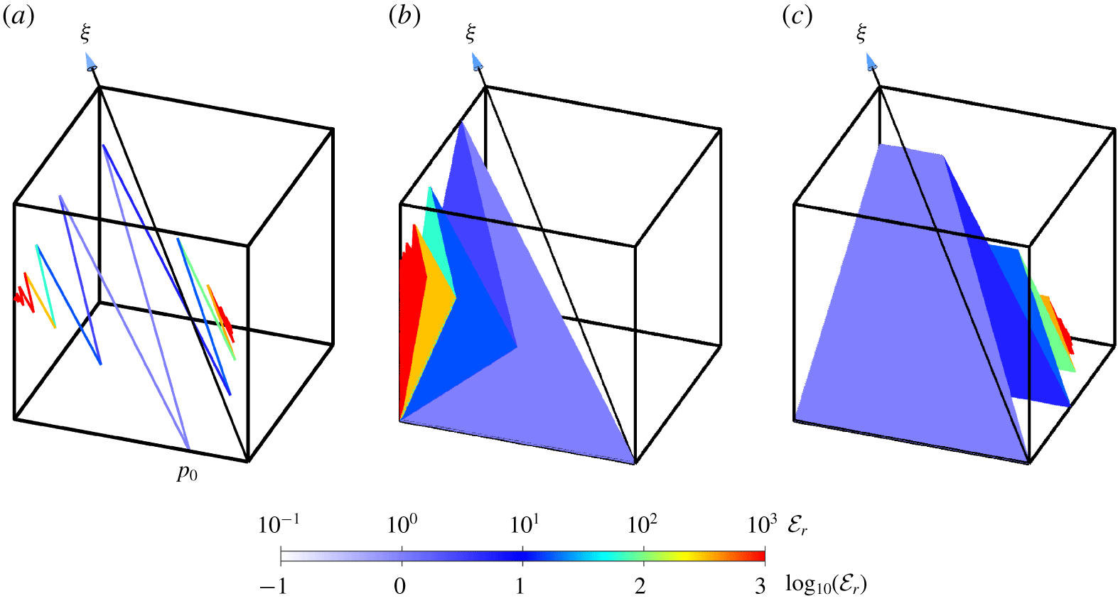
Ray tracing of beams at  $\unicode[STIX]{x1D714}=0.15$: (a) beams emitted from
 $p_{0}(-0.5,-0.25,-0.5)$ in directions
 $\boldsymbol{a}_{\pm }$ and focusing on points on two tropical edges; (b) edgebeam emitted from all
 $p_{0}(-0.5,y,-0.5)$ in direction
 $\boldsymbol{a}_{+}$; and (c) partner edgebeam emitted from the same edge but in direction
 $\boldsymbol{a}_{-}$. The beams are colour coded with the relative enstrophy
 ${\mathcal{E}}_{r}$.
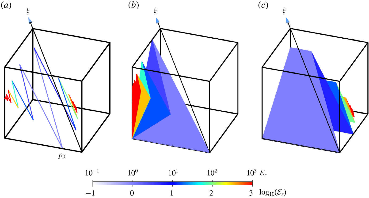
In the supercritical reflection regime, wavebeams are emitted from polar edges and focus on tropical edges. As noted in § 4.1, each point on a polar edge emits two beams in directions  $\boldsymbol{a}_{\pm }$ which focus on two different tropical edges. Figure 8(a) shows the directions
 $\boldsymbol{a}_{\pm }$ for a pair of such beams with
 $\unicode[STIX]{x1D714}=0.15$ that are emitted from a point
 $p_{0}$ on a polar edge in the southern hemisphere. The beam in the direction of
 $\boldsymbol{a}_{+}=(\unicode[STIX]{x1D6FD}_{+},1,1)$ hits the wall
 $y=0.5$, with unit normal
 $\widehat{\boldsymbol{n}}=\pm (0,1,0)$, at
 $p_{1}$. The beam is reflected at
 $p_{1}$ to a point
 $p_{2}$ on the wall
 $x=-0.5$ with unit normal
 $\widehat{\boldsymbol{n}}=\pm (1,0,0)$. The beam continues to reflect alternately on the
 $y=0.5$ and
 $x=-0.5$ walls, leading to a sequence of points
 $p_{i}$. This sequence converges towards a point
 $p_{\infty }(-0.5,0.5,z_{\infty })$ located on a tropical edge. The beam in the direction
 $\boldsymbol{a}_{-}=(\unicode[STIX]{x1D6FD}_{-},1,1)$ hits the wall
 $x=0.5$ at a point very close to the polar edge
 $x=y=0.5$, and following repeated reflections focuses on a point
 $(0.5,y_{\infty },-0.5)$ on another tropical edge. The beams are coloured with the relative enstrophy
 ${\mathcal{E}}_{r}$, assuming that
 ${\mathcal{E}}_{r}=1$ when the beam is initially emitted. Wavebeams emitted from other points
 $p_{0}$ on the same polar edge travel in parallel directions
 $\boldsymbol{a}_{\pm }$, forming two edgebeams. The edgebeam associated with
 $\boldsymbol{a}_{+}$ and its reflections are shown in figure 8(b) and the edgebeam associated with
 $\boldsymbol{a}_{-}$ and its reflections are shown in figure 8(c). The edgebeam associated with
 $\boldsymbol{a}_{+}$ focuses on a single tropical edge at
 $x=-0.5,~y=0.5$, while the edgebeam associated with
 $\boldsymbol{a}_{-}$ focuses on either one of two tropical edges,
 $x=z=-0.5$ and
 $y=0.5,~z=-0.5$, depending on the point of emission
 $p_{0}$ on the emitting polar edge. All six polar edges emit such edgebeams, for a total of 12 edgebeams. These edgebeams remain planar after each reflection. In the
 $\unicode[STIX]{x1D714}^{2}<1/3$ regime, they do not self-intersect, but they do intersect each other. This results in a complicated web of edgebeams that is difficult to visualize in a three-dimensional projected plot.
In this  $\unicode[STIX]{x1D714}^{2}$ regime, the conical beams emitted from the tropical vertices are all outside the cube, while one side of each polar double cone is completely inside the cube. The beams emitted on this cone focus onto all tropical edges, which receives contributions from both poles. For small
 $\unicode[STIX]{x1D714}$, the beams only focus on the central part of the edges, and as
 $\unicode[STIX]{x1D714}\rightarrow 1/3$, the focusing is onto the entire edge. One-sixth of each cone focuses onto one of the six polar edges, and the coverage of the edges varies continuously with the direction of emission around the cone.
4.4 The subcritical edge-focusing reflection regime: $1/3<\unicode[STIX]{x1D714}^{2}<2/3$

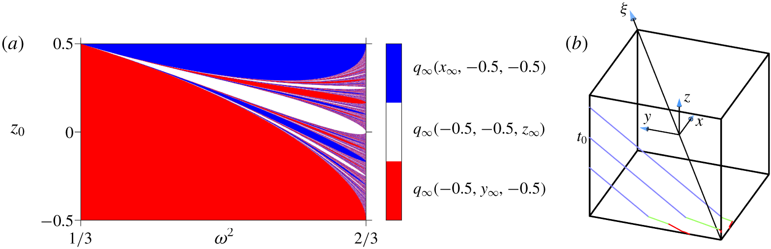
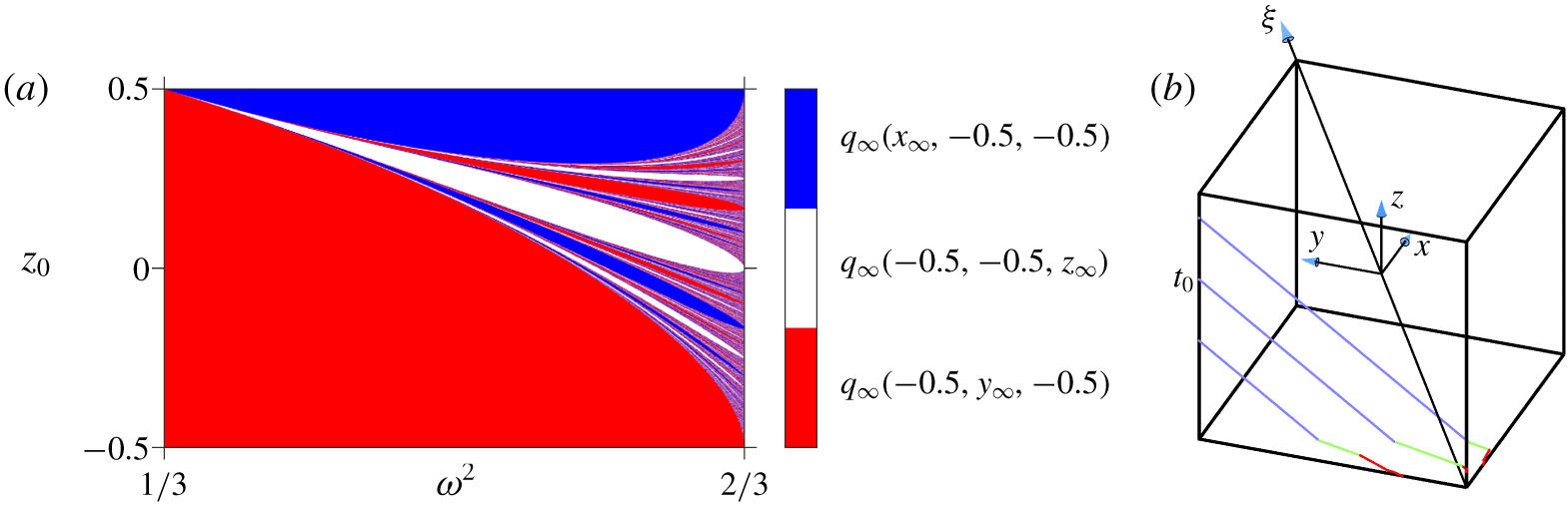
(a) Map of which polar edge,  $(x,-0.5,-0.5)$ (blue),
 $(-0.5,-0.5,z)$ (white) or
 $(-0.5,y,-0.5)$ (red), a tropical edgebeam emitted from a point
 $t_{0}(-0.5,0.5,z_{0})$ focuses onto, depending on
 $\unicode[STIX]{x1D714}^{2}\in (1/3,2/3)$ and
 $z_{0}$. (b) Ray tracing of three beams emitted from
 $t_{0}(-0.5,0.5,z)$ with
 $z=-0.1$, 0.15 and 0.4 in direction
 $-\boldsymbol{a}_{+}$, for
 $\unicode[STIX]{x1D714}=0.75$. The three beams focus on three distinct polar edges.
In the subcritical reflection regime, with  $1/3<\unicode[STIX]{x1D714}^{2}<2/3$, the polar edges emit wavebeams inside the cube only in the direction associated with
 $\boldsymbol{a}_{-}$, while for the tropical edges the wavebeams emitted inside the cube are associated with
 $-\boldsymbol{a}_{+}$. For this
 $\unicode[STIX]{x1D714}^{2}$ regime, beams emitted from points
 $t_{0}(-0.5,0.5,z_{0})$ on a tropical edge in direction
 $-\boldsymbol{a}_{+}$ focus on points
 $t_{\infty }$ on one of the three polar edges connected to the south pole. Which polar edge contains
 $t_{\infty }$ depends on
 $z_{0}$ and
 $\unicode[STIX]{x1D714}^{2}$ in a complicated fashion. Figure 9(a) uses a colour code to designate which polar edge contains the limit point:
 $(x,-0.5,-0.5)$ in blue,
 $(-0.5,-0.5,z)$ in white or
 $(-0.5,y,-0.5)$ in red. Beams emitted from lower
 $z_{0}$ positions on the tropical edge focus on the adjacent polar edge (
 $x=z=-0.5$; red), while beams emitted from higher positions focus on the opposite polar edge (
 $y=z=-0.5$; blue). In particular, a beam emitted from a point
 $t_{0}(-0.5,0.5,z_{0})$ with
 $z_{0}$ arbitrarily close to
 $0.5$ reflects on the face
 $z=-0.5$ of the cube at a point
 $t_{1}$ close to
 $(-0.5-\unicode[STIX]{x1D6FD},-0.5,-0.5)$, with
 $\unicode[STIX]{x1D6FD}=\unicode[STIX]{x1D6FD}(\unicode[STIX]{x1D714}^{2})$ decreasing from
 $\unicode[STIX]{x1D6FD}(1/3)=0$ to
 $\unicode[STIX]{x1D6FD}(2/3)=-0.5$ (see figure 4). Successive reflections alternate between the faces
 $y=-0.5$ and
 $z=-0.5$, with
 $t_{i}$ converging to
 $t_{\infty }(-0.5-\unicode[STIX]{x1D6FD},-0.5,-0)$. Upon convergence, the reflected wavevectors align with a direction orthogonal to the edge, and the corresponding wavebeam aligns with the edge itself. This edge remains outside the dual cone defined by (4.6), and the beam is trapped in the edge-focusing process. For intermediate initial abscissa
 $z_{0}$, which polar edge contains
 $t_{\infty }$ follows a fractal pattern. Beams emitted from three distinct points
 $t_{0}(-0.5,0.5,z_{0})$, with
 $z_{0}=-0.1$,
 $0.15$ and
 $0.4$, are traced in figure 9(b) for
 $\unicode[STIX]{x1D714}=0.75$ (
 $\unicode[STIX]{x1D714}^{2}\approx 0.56$). These beams eventually focus on three distinct polar edges. All six polar edges where beams focus correspond to large wavevector and velocity magnitudes
 $|\boldsymbol{k}|$ and
 $|\boldsymbol{a}|$. The sensitive dependence on the initial abscissa
 $z_{0}$ for the determination of which edge the beams focus on is reminiscent of the chaos reported in Maas (Reference Maas2005) and Pillet et al. (Reference Pillet, Maas and Dauxois2019) for wavebeam reflections in some geometries. Beams emitted from the polar edge at
 $p_{0}(-0.5,y_{0},-0.5)$ in direction
 $\boldsymbol{a}_{-}$ focus, in a similar way, to a point on one of the three polar edges connected to the north pole.
In this regime, conical beams from one side of the double cone are partially inside the cube for all vertices. The conical beams emitted from the south (north) pole focus onto northern (southern) polar edges. As  $\unicode[STIX]{x1D714}^{2}$ is increased, the portion of the edge that is focused onto recedes towards the pole, until
 $\unicode[STIX]{x1D714}^{2}\approx 5/9$, and the trend is reversed on further increasing
 $\unicode[STIX]{x1D714}^{2}$. The conical beams from the southern (northern) tropical vertices focus onto parts of the northern (southern) polar edges that include the poles. The coverage is varied; the two polar edges closest to the emitting tropical vertex are more covered by the focusing than the third polar edge. As
 $\unicode[STIX]{x1D714}^{2}\rightarrow 2/3$, the two closest edges are completely covered while the third edge is only half-covered.
4.5 The subcritical pole-focusing reflection regime: $2/3<\unicode[STIX]{x1D714}^{2}<1$

At  $\unicode[STIX]{x1D714}^{2}=2/3$, the polar edges become tangent to the dual cone (4.6). At larger
 $\unicode[STIX]{x1D714}^{2}$, a gradually increasing portion of the cube along the polar edges towards the poles falls inside the dual cone, providing an escape route for beams towards the poles. In the subcritical reflection regime
 $2/3<\unicode[STIX]{x1D714}^{2}<1$, the wavebeams are emitted from tropical edges in both directions
 $-\boldsymbol{a}_{\pm }$ but focus on poles rather than polar edges. For
 $\unicode[STIX]{x1D714}^{2}<8/9$, all beams emitted from points on the tropical edge
 $(-0.5,0.5,z_{0})$ in the direction
 $-\boldsymbol{a}_{+}$ point to the face at
 $z=-0.5$. For
 $\unicode[STIX]{x1D714}^{2}>8/9$, the situation is different. The beam first impacts the face
 $x=0.5$ at a point
 $t_{1}$, and is reflected. The reflection is subcritical and the beam is further reflected by the faces
 $x=-0.5$,
 $y=-0.5$ and
 $z=-0.5$. Eventually, the beam converges to the south pole. The beam emitted in the direction
 $-\boldsymbol{a}_{-}$ likewise eventually focuses on the north pole.
In this regime, the conical beams emitted from the poles are completely outside the cube. The conical beams from one side of the double cones emitted from southern (northern) tropical vertices all focus onto the north (south) pole.
4.6 Convergence rates for focusing
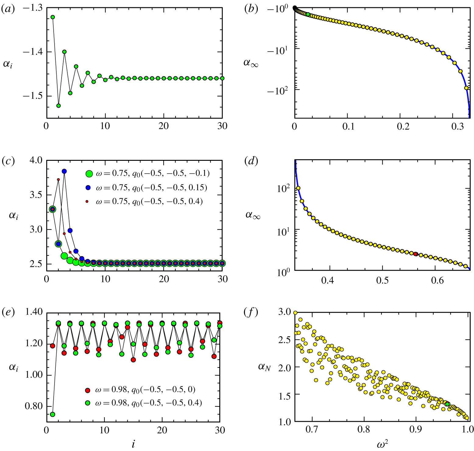
Sequence of wavevector ratios: (a)  $\unicode[STIX]{x1D6FC}_{i}<0$, obtained after
 $i$ reflections versus
 $i$ for
 $\unicode[STIX]{x1D714}=0.15$ and wavebeam originating from
 $p_{0}(-0.5,-0.25,-0.5)$ in direction
 $\boldsymbol{a}_{+}$; (c)
 $\unicode[STIX]{x1D6FC}_{i}>0$, obtained after
 $i$ reflections versus
 $i$ for
 $\unicode[STIX]{x1D714}=0.75$ and wavebeam originating from
 $q_{0}$ as indicated in direction
 $-\boldsymbol{a}_{+}$; and (e)
 $\unicode[STIX]{x1D6FC}_{i}>0$, obtained after
 $i$ reflections versus
 $i$ for
 $\unicode[STIX]{x1D714}=0.98$ and wavebeam originating from
 $q_{0}$ as indicated in direction
 $-\boldsymbol{a}_{+}$. The limit ratios (b)
 $\unicode[STIX]{x1D6FC}_{\infty }<0$ and (d)
 $\unicode[STIX]{x1D6FC}_{\infty }>0$ upon focusing of wavebeams versus
 $\unicode[STIX]{x1D714}^{2}$. The blue curve is the explicit expression of the limit given by (4.25), and the yellow symbols are the limits obtained numerically after a large number of reflections. The green and red symbols correspond to the cases in (a) and (c). (f) The ratio
 $\unicode[STIX]{x1D6FC}_{N}$ after a number
 $N$ of reflections guaranteeing convergence of
 $q_{i}$ within a small prescribed distance from the south pole, for a beam emitted from
 $q_{0}(-0.5,0.5,0)$, versus
 $\unicode[STIX]{x1D714}^{2}$. The red and green symbols correspond to the cases in (e).
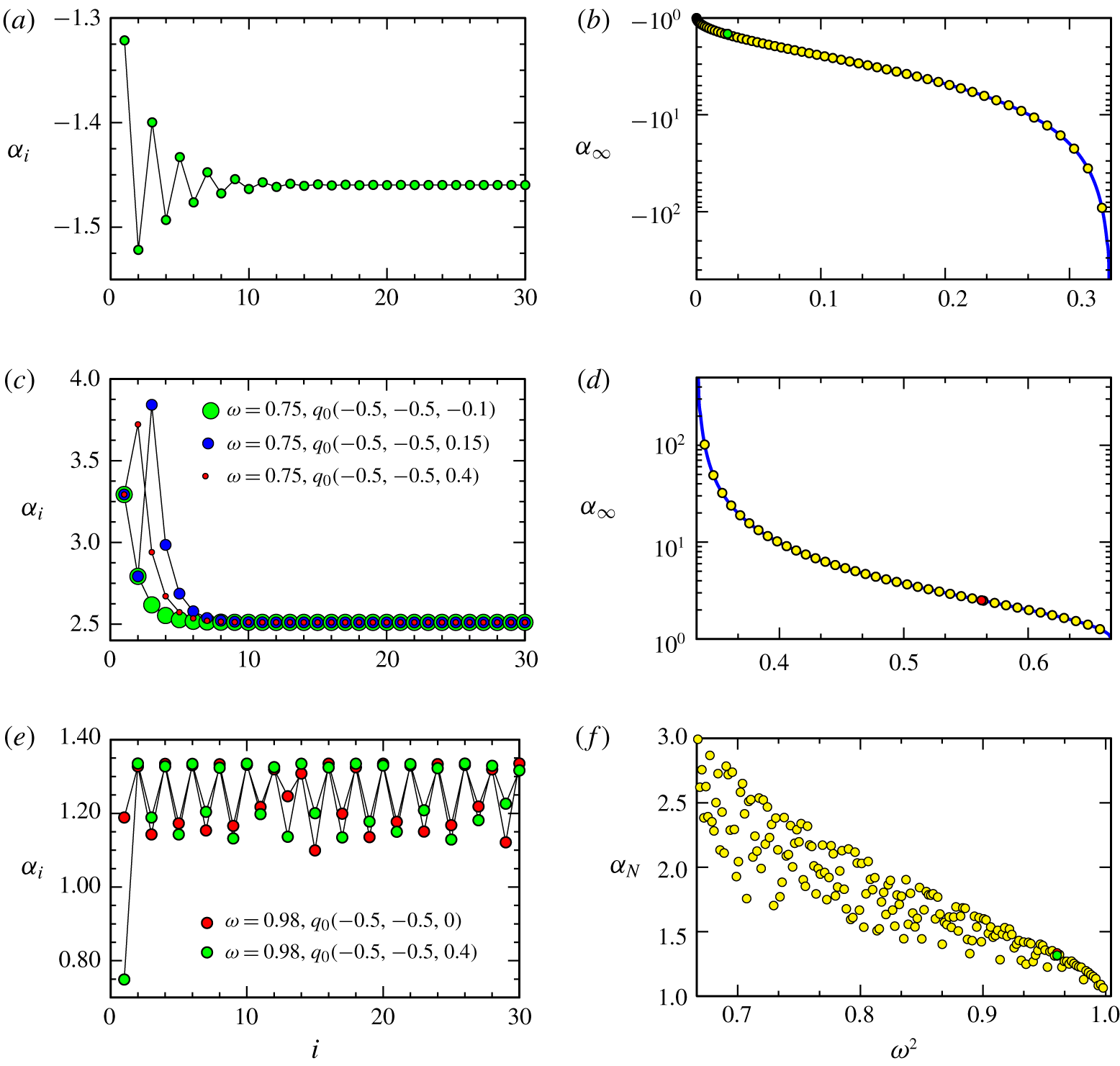
We now consider the rate at which edgebeams focus onto either edges or poles. We only consider emissions associated with the  $\pm \boldsymbol{a}_{+}$ direction, as these will be seen in the simulations (DNS) to be more energetic than their counterparts emitted in the
 $\pm \boldsymbol{a}_{-}$ direction. A beam emitted from a point arbitrarily close to the south pole converges to the point
 $p_{\infty }(-0.5,0.5,z_{\infty }^{max})$, with
 $z_{\infty }^{max}\approx 0.2421$ at
 $\unicode[STIX]{x1D714}=0.15$, so that the transformation
 $p_{0}\rightarrow p_{\infty }$ maps the polar edge to only part of the tropical edge. As
 $\unicode[STIX]{x1D714}^{2}$ increases from
 $0$ to
 $1/3$,
 $z_{\infty }^{max}$ increases from approximately
 $0.2320$ to
 $0.5000$. The sequence of reflected-to-incident wavevector ratios
 $\unicode[STIX]{x1D6FC}_{i}$ also converges to a limit
 $\unicode[STIX]{x1D6FC}_{\infty }\approx -1.4597$ for
 $\unicode[STIX]{x1D714}=0.15$, as illustrated in figure 10(a). This limit is independent of the choice of initial point
 $p_{0}$ on the polar edge because the reflections always alternate between the same two faces,
 $y=0.5$ and
 $x=-0.5$. Reflections on the face
 $y=0.5$ are associated with a decreasing sub-sequence of ratios
 $\unicode[STIX]{x1D6FC}_{2i-1}$, while reflections on the face
 $x=-0.5$ are associated with an increasing sub-sequence of ratios
 $\unicode[STIX]{x1D6FC}_{2i}$. This behaviour generalizes to all
 $\unicode[STIX]{x1D714}^{2}<1/3$. An explicit expression for
 $\unicode[STIX]{x1D6FC}_{\infty }$ as a function of
 $\unicode[STIX]{x1D714}^{2}$,
 $$\begin{eqnarray}\unicode[STIX]{x1D6FC}_{\infty }=\frac{1+\sqrt{3\unicode[STIX]{x1D714}^{2}(2-3\unicode[STIX]{x1D714}^{2})}}{3\unicode[STIX]{x1D714}^{2}-1},\end{eqnarray}$$
can be derived from the matrix representation of the composition of two successive reflections (see appendix C for a proof). In figure 10(b), the blue curve is a plot of  $\unicode[STIX]{x1D6FC}_{\infty }(\unicode[STIX]{x1D714}^{2})$ from (4.25) and the yellow symbols are the values of
 $\unicode[STIX]{x1D6FC}_{\infty }$ estimated by numerically tracking a large number of reflections. The sequence
 $\unicode[STIX]{x1D6FC}_{i}$ converges to
 $\unicode[STIX]{x1D6FC}_{\infty }$ geometrically. The convergence rate
 $1/|\unicode[STIX]{x1D6FC}_{\infty }|$ is the ratio of the eigenvalues of the matrix representation of the reflection mapping incident to reflected wavevectors; see appendix C, where it is also observed that the sequence of reflected unit wavevectors converges to a unit vector orthogonal to the edge containing the focusing point
 $t_{\infty }$, and the corresponding group velocity direction
 $\widehat{\boldsymbol{a}}$ aligns itself with the edge.
After each reflection  $|\boldsymbol{c}_{g}^{\prime }|/|\boldsymbol{c}_{g}|=|\boldsymbol{k}|/|\boldsymbol{k}^{\prime }|=1/|\unicode[STIX]{x1D6FC}|$, hence the beam’s group velocity decreases at the same rate as its wavelength,
 $1/|\unicode[STIX]{x1D6FC}|$. Upon focusing, the distance between two reflections also decreases at approximately the same rate
 $1/|\unicode[STIX]{x1D6FC}|$, so that the time it takes for the energy to propagate between consecutive reflections remains approximately constant, and hence it takes an infinite travel time to reach the focus point. This was already observed by Greenspan (Reference Greenspan1969) in the context of the two-dimensional wedge.
Although which polar edge an emitted beam focuses on depends chaotically on the point of emission  $z_{0}$ when
 $1/3<\unicode[STIX]{x1D714}^{2}<2/3$, the convergence rate for a given
 $\unicode[STIX]{x1D714}$ is independent of
 $z_{0}$. Figure 10(c) illustrates this for three different
 $z_{0}$ at
 $\unicode[STIX]{x1D714}=0.75$; after approximately a dozen reflections, the wavevector ratios
 $\unicode[STIX]{x1D6FC}_{i}$ converge to the same value
 $\unicode[STIX]{x1D6FC}_{\infty }\approx 2.5$. Figure 10(d) plots the limit values
 $\unicode[STIX]{x1D6FC}_{\infty }$ for
 $1/3<\unicode[STIX]{x1D714}^{2}<2/3$ obtained from EBA (yellow symbols). The underlying blue curve is the explicit expression of the limit given by (4.25). This
 $\unicode[STIX]{x1D6FC}_{\infty }(\unicode[STIX]{x1D714}^{2})$ is related to
 $\unicode[STIX]{x1D6FC}_{\infty }$ for
 $\unicode[STIX]{x1D714}^{2}<1/3$, shown in figure 10(b), via the symmetry relation
 $\unicode[STIX]{x1D6FC}_{\infty }(2/3-\unicode[STIX]{x1D714}^{2})=-\unicode[STIX]{x1D6FC}_{\infty }(\unicode[STIX]{x1D714}^{2})$.
For  $\unicode[STIX]{x1D714}^{2}>8/9$, there seems to be no clear pattern in the sequence of faces the beam is reflecting off. This apparently more erratic convergence behaviour of the beam, compared to the supercritical reflections for
 $\unicode[STIX]{x1D714}^{2}<1/3$, also features in the sequence of energy ratios
 $|\unicode[STIX]{x1D6FC}|$ at each reflection, which does not converge in a pointwise sense, as illustrated in figures 10(e,f).
The beams making up a conical vertex beam follow exactly the same convergence behaviour as the edgebeams just described, except for beams from the cone that are emitted into certain symmetry planes. These are considered in the next section.
4.7 Vertex beams in symmetry planes
In this section, we consider the special cases of the wavebeams from vertices that are emitted in the symmetry plane  $y=z$ (with similar behaviour in the other two symmetry planes,
 $x=y$ and
 $x=z$). The normal vectors to the cube’s walls in the symmetry plane
 $y=z$, which contains the axis of rotation, are coplanar, and an incident beam whose group velocity is in that plane is reflected into a beam whose group velocity is in the same plane (a two-dimensional reflection). These normal vectors are
 $\widehat{\boldsymbol{n}}=(1,0,0)$ for the walls at
 $x=\pm 0.5$ and
 $\widehat{\boldsymbol{n}}=(0,1,1)/\sqrt{2}$ for the edges
 $y=z=\pm 0.5$. These vertex beams have qualitatively different behaviour in four
 $\unicode[STIX]{x1D714}^{2}$ regimes.
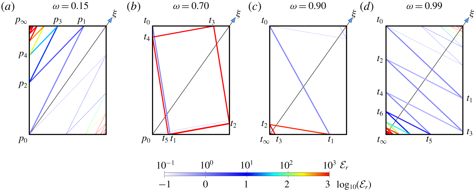
Reflections in the plane  $y=z$ of beams emitted from (a) the south pole
 $p_{0}$, (b) the south pole
 $p_{0}$ and the tropical vertex
 $t_{0}(-0.5,0.5,0.5)$, (c,d) the tropical vertex
 $t_{0}(-0.5,0.5,0.5)$, at
 $\unicode[STIX]{x1D714}$ as indicated. The colour of the beam indicates its relative enstrophy
 ${\mathcal{E}}_{r}$. All beams are initially emitted with
 ${\mathcal{E}}_{r}=1$. The view is from a direction orthogonal to the plane
 $y=z$, with the horizontal boundaries being polar edges and the vertical boundaries being lines
 $y=z$ on the cube faces
 $x=\pm 0.5$. Thick (thin) lines correspond to beams emitted in direction
 $\pm \boldsymbol{a}_{+}$ (
 $\pm \boldsymbol{a}_{-}$).
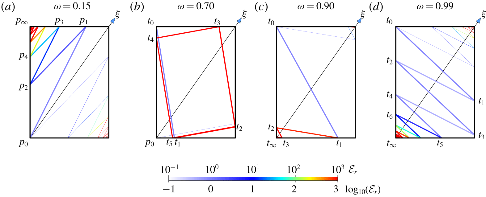
For  $\unicode[STIX]{x1D714}^{2}<1/3$, a vertex beam emitted from the south pole
 $p_{0}(-0.5,-0.5,-0.5)$ in a direction
 $\boldsymbol{a}_{+}=(\unicode[STIX]{x1D6FD}_{+},1,1)$ is reflected at a point
 $p_{1}(\unicode[STIX]{x1D6FD}_{+}-0.5,0.5,0.5)$ on the edge
 $y=z=0.5$ (see figure 11a), with
 $\unicode[STIX]{x1D6FD}_{+}$ given by (4.9). The beam reflected at
 $p_{1}$ travels in the direction
 $-\boldsymbol{a}_{-}$ to a point
 $p_{2}(-0.5,0.5-\unicode[STIX]{x1D6FD}_{2},0.5-\unicode[STIX]{x1D6FD}_{2})$ where it meets the face
 $x=-0.5$ of the cube. Rather than using (4.11), the value of
 $\unicode[STIX]{x1D6FD}_{2}$ can be obtained directly by enforcing (4.6) for
 $\boldsymbol{a}=-\boldsymbol{a}_{-}\propto \overrightarrow{p_{1}p_{2}}$, namely
 $$\begin{eqnarray}(\unicode[STIX]{x1D6FD}_{+}+2\unicode[STIX]{x1D6FD}_{2})^{2}=3(1-\unicode[STIX]{x1D714}^{2})(\unicode[STIX]{x1D6FD}_{+}^{2}+2\unicode[STIX]{x1D6FD}_{2}^{2}).\end{eqnarray}$$
Dividing (4.26) by  $\unicode[STIX]{x1D6FD}_{2}^{2}$ yields the quadratic equation (4.8) with
 $\unicode[STIX]{x1D6FD}$ replaced by
 $\unicode[STIX]{x1D6FD}=\unicode[STIX]{x1D6FD}_{+}/\unicode[STIX]{x1D6FD}_{2}$. The two roots of (4.26) are
 $\unicode[STIX]{x1D6FD}_{2}=1$ and
 $\unicode[STIX]{x1D6FD}_{2}=\unicode[STIX]{x1D6FE}$, with
 $$\begin{eqnarray}\unicode[STIX]{x1D6FE}=\unicode[STIX]{x1D6FD}_{+}/\unicode[STIX]{x1D6FD}_{-}.\end{eqnarray}$$
The root  $\unicode[STIX]{x1D6FD}_{2}=1$ (taking
 $\unicode[STIX]{x1D6FD}=\unicode[STIX]{x1D6FD}_{+}$) corresponds to the incident beam and the root
 $\unicode[STIX]{x1D6FD}_{2}=\unicode[STIX]{x1D6FE}$ (taking
 $\unicode[STIX]{x1D6FD}=\unicode[STIX]{x1D6FD}_{-}$) corresponds to the reflected beam. Successive reflections occur at points
 $p_{2i+1}(\unicode[STIX]{x1D6FD}_{2i+1}-0.5,0.5,0.5)$ on the polar edge
 $y=z=0.5$ and
 $p_{2i+2}(-0.5,0.5-\unicode[STIX]{x1D6FD}_{2i+2},0.5-\unicode[STIX]{x1D6FD}_{2i+2})$ on the face
 $x=-0.5$, for
 $i>0$. An argument similar to that used to obtain
 $\unicode[STIX]{x1D6FD}_{2}$ yields
 $\unicode[STIX]{x1D6FD}_{2i+1}/\unicode[STIX]{x1D6FD}_{2i}=\unicode[STIX]{x1D6FD}_{+}$ and
 $\unicode[STIX]{x1D6FD}_{2i+1}/\unicode[STIX]{x1D6FD}_{2i+2}=\unicode[STIX]{x1D6FD}_{-}$, from which
 $$\begin{eqnarray}\unicode[STIX]{x1D6FD}_{2i}=\unicode[STIX]{x1D6FE}^{i}\quad \text{and}\quad \unicode[STIX]{x1D6FD}_{2i+1}=\unicode[STIX]{x1D6FD}_{+}\unicode[STIX]{x1D6FD}_{2i}=\unicode[STIX]{x1D6FD}_{+}\unicode[STIX]{x1D6FE}^{i},\quad i\geqslant 0.\end{eqnarray}$$
In particular,  $\unicode[STIX]{x1D6FD}_{i}\rightarrow 0$ geometrically at the rate
 $\unicode[STIX]{x1D6FE}^{1/2}\in (0,1)$ and
 $p_{i}\rightarrow p_{\infty }(-0.5,0.5,0.5)$, a tropical vertex, as
 $i\rightarrow \infty$. In contrast, the rate
 $1/|\unicode[STIX]{x1D6FC}_{\infty }|$ for three-dimensional reflections is only asymptotically geometric. Pillet et al. (Reference Pillet, Maas and Dauxois2019) also found geometric convergence for the focusing of wavebeams onto a two-dimensional limit cycle attractor in their translationally invariant prismatic configuration. This type of convergence is ultimately related to the normals of the reflecting walls involved being coplanar.
For  $1/3<\unicode[STIX]{x1D714}^{2}<2/3$, the beam emitted from the tropical vertex
 $t_{0}(-0.5,0.5,0.5)$ is cyclically reflected on the polar edge
 $y=z=-0.5$, then the face
 $x=0.5$, then the polar edge
 $y=z=0.5$, and then the face
 $x=-0.5$ of the cube, at a sequence of points
 $t_{4i+1}(\unicode[STIX]{x1D6FD}_{4i+1}-0.5,-0.5,-0.5)$,
 $t_{4i+2}(0.5,\unicode[STIX]{x1D6FD}_{4i+2}-0.5,\unicode[STIX]{x1D6FD}_{4i+2}-0.5)$,
 $t_{4i+3}(0.5-\unicode[STIX]{x1D6FD}_{4i+3},0.5,0.5)$ and
 $t_{4i+4}(-0.5,0.5-\unicode[STIX]{x1D6FD}_{4i+4},0.5-\unicode[STIX]{x1D6FD}_{4i+4})$, for
 $i\geqslant 0$ (see figure 11b). The same argument as was used for
 $\unicode[STIX]{x1D714}^{2}<1/3$ shows that the successive terms of the sequence
 $\{\unicode[STIX]{x1D6FD}_{i}\}$ must be related via
 $$\begin{eqnarray}\unicode[STIX]{x1D6FD}_{4i+1}/(\unicode[STIX]{x1D6FD}_{4i}-1)=\unicode[STIX]{x1D6FD}_{4i+3}/(\unicode[STIX]{x1D6FD}_{4i+2}-1)=\unicode[STIX]{x1D6FD}_{+}\end{eqnarray}$$
and
 $$\begin{eqnarray}(1-\unicode[STIX]{x1D6FD}_{4i+1})/\unicode[STIX]{x1D6FD}_{4i+2}=(1-\unicode[STIX]{x1D6FD}_{4i+3})/\unicode[STIX]{x1D6FD}_{4i+4}=\unicode[STIX]{x1D6FD}_{-},\end{eqnarray}$$
so that  $\overrightarrow{t_{4i}t_{4i+1}}$ and
 $\overrightarrow{t_{4i+2}t_{4i+3}}$ align with
 $(\unicode[STIX]{x1D6FD}_{+},1,1)$, and
 $\overrightarrow{t_{4i+1}t_{4i+2}}$ and
 $\overrightarrow{t_{4i+3}t_{4i+4}}$ align with
 $(\unicode[STIX]{x1D6FD}_{-},1,1)$. The relations (4.29) combine into a linear recurrence relation for
 $\{{\unicode[STIX]{x1D6FD}_{4i}\}}_{i\geqslant 0}$,
 $$\begin{eqnarray}\unicode[STIX]{x1D6FD}_{4(i+1)}=\unicode[STIX]{x1D6FE}^{2}\unicode[STIX]{x1D6FD}_{4i}+(1-\unicode[STIX]{x1D6FE})(\unicode[STIX]{x1D6FE}+1/\unicode[STIX]{x1D6FD}_{-}),\end{eqnarray}$$
with  $-1<\unicode[STIX]{x1D6FE}<0$. From this recurrence relation, we have
 $\unicode[STIX]{x1D6FD}_{4i}\rightarrow (\unicode[STIX]{x1D6FE}+1/\unicode[STIX]{x1D6FD}_{-})/(\unicode[STIX]{x1D6FE}+1)\in (0,1)$ as
 $i\rightarrow \infty$ at the rate
 $\unicode[STIX]{x1D6FE}^{2}$, and
 $(\unicode[STIX]{x1D6FD}_{2i},\unicode[STIX]{x1D6FD}_{2i+1})\rightarrow (1+\unicode[STIX]{x1D6FD}_{+},\unicode[STIX]{x1D6FD}_{+}[1-\unicode[STIX]{x1D6FD}_{-}])/(\unicode[STIX]{x1D6FD}_{+}+\unicode[STIX]{x1D6FD}_{-})$ at the rate
 $|\unicode[STIX]{x1D6FE}|$. The beam thus focuses onto a limit cycle in the plane
 $y=z$, at the same rate as the beam focuses to a tropical vertex in the supercritical regime
 $\unicode[STIX]{x1D714}^{2}<1/3$,
 $|\unicode[STIX]{x1D6FE}|^{1/2}$ on average per reflection. Figure 11(b) shows that the focusing occurring in this
 $\unicode[STIX]{x1D714}^{2}$ regime is extremely rapid. In fact,
 $|\unicode[STIX]{x1D6FE}|$ vanishes at
 $\unicode[STIX]{x1D714}^{2}=1/3$ and
 $\unicode[STIX]{x1D714}^{2}=2/3$, and has maximal value
 $17-12\sqrt{2}\approx 0.03$ at
 $\unicode[STIX]{x1D714}^{2}=1/2$. This limit cycle is a saddle, not an attractor. The
 $y=z$ plane is its stable manifold. Any beam emitted from a point on an edge arbitrarily close to the vertex in the plane will propagate away from the plane.
The regime  $\unicode[STIX]{x1D714}^{2}>2/3$ is comparable to the supercritical regime
 $\unicode[STIX]{x1D714}^{2}<1/3$ for the two-dimensional reflections in the plane
 $y=z$, but with alternating reflections at the polar edge
 $y=z=-0.5$ and the face
 $x=-0.5$ for the beam originating at the tropical vertex
 $t_{0}(-0.5,0.5,0.5)$, at points
 $t_{2i+1}(\unicode[STIX]{x1D6FD}_{2i+1}-0.5,-0.5,-0.5)$ and
 $t_{2i+2}(-0.5,\unicode[STIX]{x1D6FD}_{2i+2}-0.5,\unicode[STIX]{x1D6FD}_{2i+2}-0.5)$, respectively, for all
 $i\geqslant 0$ if
 $\unicode[STIX]{x1D714}^{2}<8/9$ (figure 11c), or after one or several reflections on the wall at
 $x=+0.5$ if
 $\unicode[STIX]{x1D714}^{2}>8/9$ (figure 11d). In the latter case, reflections at
 $t_{1}$ on the wall
 $x=+0.5$ are accompanied by a decrease of the wavevector magnitude,
 $|\unicode[STIX]{x1D6FC}_{1}|<1$. The enstrophy lost in the process is regained at the next reflection at
 $t_{2}$, where
 $|\unicode[STIX]{x1D6FC}_{2}|>1$, in such a way that the enstrophy of the beam between
 $t_{2}$ and
 $t_{3}$ is exactly the same as that of the emitted beam; between
 $t_{0}$ and
 $t_{1}$,
 $\unicode[STIX]{x1D6FC}_{1}\unicode[STIX]{x1D6FC}_{2}=1$. This is a consequence of the two opposite reflecting planes at
 $x=\pm 0.5$ being parallel, with the same normal direction
 $\widehat{\boldsymbol{n}}$. The beam eventually focuses at the south pole
 $t_{\infty }(-0.5,-0.5,-0.5)$. For
 $\unicode[STIX]{x1D714}^{2}>2/3$, we have
 $\unicode[STIX]{x1D6FD}_{-}<\unicode[STIX]{x1D6FD}_{+}<0$,
 $0<\unicode[STIX]{x1D6FE}<1$, and for
 $2/3<\unicode[STIX]{x1D714}^{2}<8/9$ the expressions (4.28) read
 $$\begin{eqnarray}\unicode[STIX]{x1D6FD}_{2i}=\unicode[STIX]{x1D6FE}^{i}\quad \text{and}\quad \unicode[STIX]{x1D6FD}_{2i+1}=-\unicode[STIX]{x1D6FD}_{+}\unicode[STIX]{x1D6FD}_{2i}=-\unicode[STIX]{x1D6FD}_{+}\unicode[STIX]{x1D6FE}^{i}.\end{eqnarray}$$
The behaviour of a beam emitted from the south pole (for  $\unicode[STIX]{x1D714}^{2}<2/3$) or the tropical vertex
 $(-0.5,0.5,0.5)$ (for
 $\unicode[STIX]{x1D714}^{2}>2/3$) in the direction
 $\boldsymbol{a}_{-}=(\unicode[STIX]{x1D6FD}_{-},1,1)$ (
 $\unicode[STIX]{x1D714}^{2}<2/3$) or
 $-\boldsymbol{a}_{-}=-(\unicode[STIX]{x1D6FD}_{-},1,1)$ (
 $\unicode[STIX]{x1D714}^{2}>2/3$) is similar. This beam and its reflections are also shown in figure 11, without labelling the locations of the various reflection points and with thinner lines than the
 $\pm \boldsymbol{a}_{+}$ beams. In figures 11(a,c,d), the beam’s reflections are observed to follow a pattern which mirrors that followed by the beam emitted in the
 $\boldsymbol{a}_{+}$ (figure 11a) or
 $-\boldsymbol{a}_{+}$ (figure 11c,d) directions, with the beams associated with the
 $(\pm )\boldsymbol{a}_{\pm }$ directions focusing in opposite vertices. In figure 11(b), the beam emitted from the south pole in the
 $\boldsymbol{a}_{-}$ direction also settles onto the same limit cycle as the beam emitted from the tropical vertex in the
 $-\boldsymbol{a}_{+}$ direction, at the same rate.
5 Comparison of inviscid predictions and Navier–Stokes simulations
In this section, the inviscid EBA results are compared with the results of solving the Navier–Stokes system (2.2) in the low-Ekman-number, small-forcing-amplitude regime with  $\text{E}=10^{-7}$ and
 $\unicode[STIX]{x1D716}=10^{-7}$ (DNS). In order to appreciate the way the beams are arranged in the interior of the cube, we plot their intersections with three planes: (i) the equatorial plane
 $x+y+z=0$, whose intersection with the cube forms a perfect hexagon; (ii) a meridional plane,
 $x+y=2z$, containing the axis of rotation and passing through the midpoints of the tropical edges; and (iii) another meridional plane
 $y=z$, labelled ‘diagonal’, which contains the axis of rotation and is invariant under the symmetry
 ${\mathcal{S}}$ (4.7). The intersections of individual beams with the three planes are shown in the rows of figures 12 and 13 labelled EBA for selected frequencies in the inertial range
 $0<\unicode[STIX]{x1D714}^{2}<1$. Each panel consists of points (dots), which are drawn larger for beams originating from an edge associated with
 $\pm \boldsymbol{a}_{+}$ or a tropical vertex, and smaller for beams associated with
 $\pm \boldsymbol{a}_{-}$ or from a pole. These points form either thick or thin straight segments for edgebeams and conic sections for vertex beams, and are coloured using the relative enstrophy
 ${\mathcal{E}}_{r}$ according to the EBA scale.
Figure 12 compares the EBA and DNS results in the three planes for  $\unicode[STIX]{x1D714}^{2}<1/3$. In this range the focusing of beams onto tropical edges is apparent. In the meridional plane, we see what appears to be two pairs of rays (in blue) emitted from the north and south poles and focusing onto tropical edges. The picture is qualitatively similar for other half-frequencies with
 $\unicode[STIX]{x1D714}^{2}<1/3$; the edgebeam planes are almost parallel to the rotation axis for very small
 $\unicode[STIX]{x1D714}$ and become tangential to the faces of the cube as
 $\unicode[STIX]{x1D714}^{2}\rightarrow 1/3$. The rows of figure 12 labelled DNS consist of snapshots of the enstrophy of the Navier–Stokes computed flows with
 $\text{E}=10^{-7}$ and
 $\unicode[STIX]{x1D716}=10^{-7}$ in the same planes at the corresponding
 $\unicode[STIX]{x1D714}$, showing excellent agreement with the inviscid (
 $\text{E}=0$) unforced (
 $\unicode[STIX]{x1D716}=0$) EBA. In the DNS snapshots there is also evidence of polar conical beams whose trace in the equatorial plane forms a circular region of low-level constant enstrophy. In the EBA setting, the stronger wavebeams are zero-thickness sheets. For finite Ekman numbers, these are replaced by finite-thickness vortex sheets. The diagonal plane
 $y=z$ contains the two-dimensional reflections described in § 4.7, and the DNS results in this plane show clear evidence of these.
Local enstrophy from EBA and DNS on the equatorial plane  $x+y+z=0$ (
 $\unicode[STIX]{x1D743}$ points out of the page), a meridional plane
 $x+y=2z$ (
 $\unicode[STIX]{x1D743}$ points up in the page) and the diagonal plane
 $y=z$ (
 $\unicode[STIX]{x1D743}$ points up in the page), at
 $\unicode[STIX]{x1D714}$ as indicated. Movie 3 animates the EBA and DNS results in the three planes for
 $\unicode[STIX]{x1D714}\in (0,1)$. Movie 2 animates the DNS results in the three planes, as well as the surface, over one forcing period at select values of
 $\unicode[STIX]{x1D714}$. Thick (thin) lines are made of points corresponding to edgebeams emitted in direction
 $\pm \boldsymbol{a}_{+}$ (
 $\pm \boldsymbol{a}_{-}$) or tropical (polar) vertex beams.
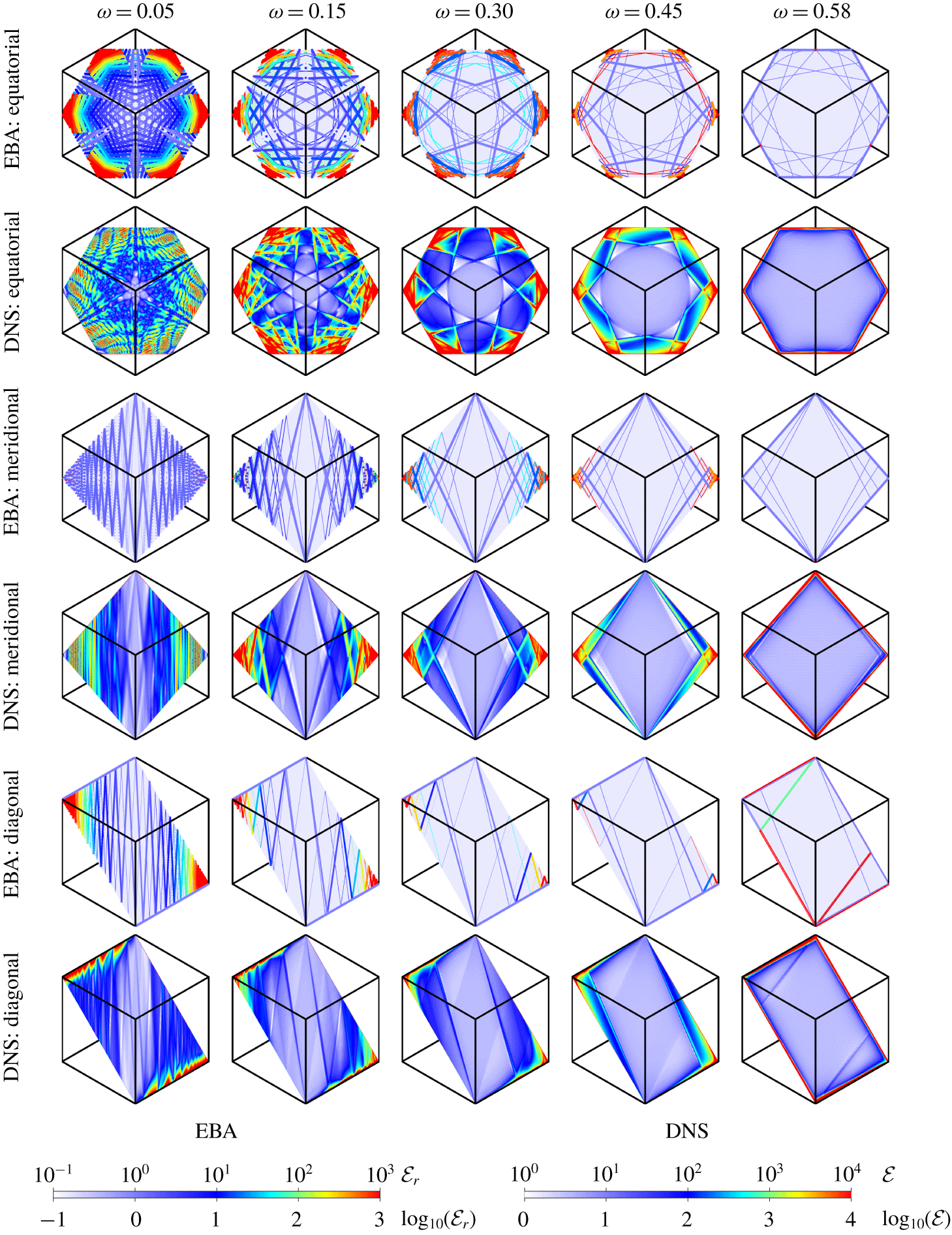
Local enstrophy from EBA and DNS on the equatorial plane  $x+y+z=0$ (
 $\unicode[STIX]{x1D743}$ points out of the page), a meridional plane
 $x+y=2z$ (
 $\unicode[STIX]{x1D743}$ points up in the page) and the diagonal plane
 $y=z$ (
 $\unicode[STIX]{x1D743}$ points up in the page), at
 $\unicode[STIX]{x1D714}$ as indicated. Movie 3 animates the EBA and DNS results in the three planes for
 $\unicode[STIX]{x1D714}\in (0,1)$. Movie 2 animates the DNS results in the three planes, as well as the surface, over one forcing period at select values of
 $\unicode[STIX]{x1D714}$. Thick (thin) lines are made of points corresponding to edgebeams emitted in direction
 $\pm \boldsymbol{a}_{+}$ (
 $\pm \boldsymbol{a}_{-}$) or tropical (polar) vertex beams.
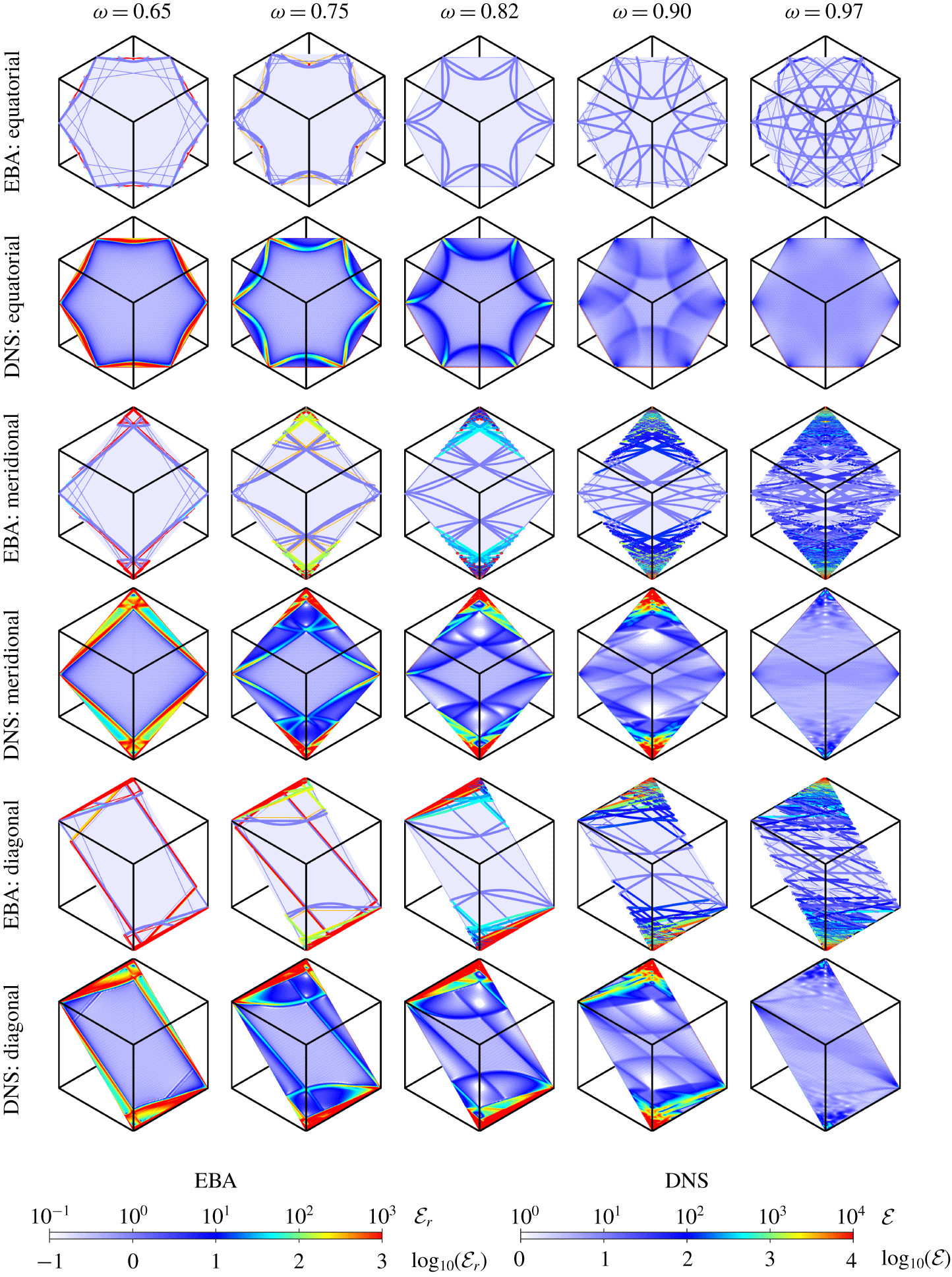
Surface enstrophy  ${\mathcal{E}}_{r}$ from EBA and snapshots of enstrophy
 ${\mathcal{E}}$ from DNS at phase
 $0$ of forcing, at
 $\unicode[STIX]{x1D714}$ as indicated. Movie 1 animates snapshots of the EBA and DNS results at the same phase over the half-frequency range
 $0.01\leqslant \unicode[STIX]{x1D714}\leqslant 0.99$ with
 $0.01$ increments in
 $\unicode[STIX]{x1D714}$; and the bottom row of movie 2 animates the DNS surface enstrophy over one libration period for several values of
 $\unicode[STIX]{x1D714}$. Thick (thin) lines are made of points corresponding to edgebeams emitted in direction
 $\pm \boldsymbol{a}_{+}$ (
 $\pm \boldsymbol{a}_{-}$) or tropical (polar) vertex beams.
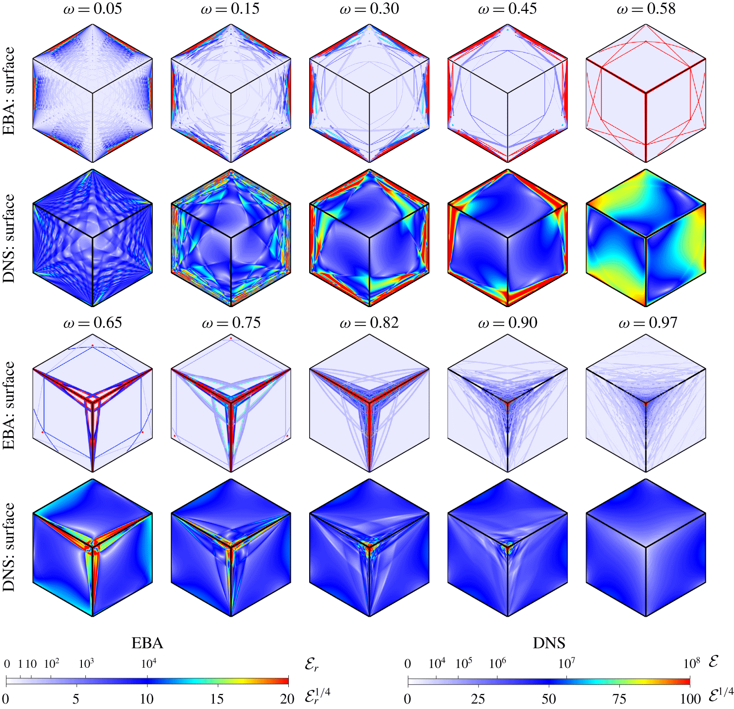
Figure 13 compares the EBA and DNS results in the three planes for  $\unicode[STIX]{x1D714}^{2}>1/3$. A noticeable bending of the internal shear layer occurs in the DNS; there is some evidence of this at lower
 $\unicode[STIX]{x1D714}^{2}<1/3$ (see figure 12), but it is not as pronounced. This bending is principally due to the conical beams emitted from the tropical vertices and, to a lesser extent, the breaking of the time-reversal symmetry
 ${\mathcal{S}}$ by the viscous terms in the Navier–Stokes equations and the resulting change in the direction in which wavebeams are emitted. These viscous effects are akin to what happens to beams emitted from an edge in a rotating cylinder: in the viscous setting the emitted rays no longer form a perfect double cone but rather a hyperboloid of one sheet whose cross-section with a meridional plane is no longer a St. Andrew’s cross but two branches of a hyperbola. At the low Ekman number
 $\text{E}=10^{-7}$ used in the simulations, the contribution from the breaking of
 ${\mathcal{S}}$ symmetry is relatively weak.
Even at the surface of the cube, the inviscid EBA and the Navier–Stokes DNS simulations compare very well, as can be seen from figure 14 showing the relative surface enstrophies from EBA and snapshots at phase 0 of the librational forcing from the DNS at various half-frequencies  $\unicode[STIX]{x1D714}$. The criss-crossing pattern at the surface of the cube for small
 $\unicode[STIX]{x1D714}$ observed in the DNS, mentioned earlier in § 3.1, is very well captured by the EBA results, as are the focusing and enhanced enstrophy on the tropical edges for
 $\unicode[STIX]{x1D714}^{2}<1/3$, the focusing and enhanced enstrophy on the polar edges for
 $\unicode[STIX]{x1D714}^{2}>1/3$, and the transition to focusing on the poles as
 $\unicode[STIX]{x1D714}^{2}\rightarrow 8/9$. Movie 1 shows both the EBA and DNS surface enstrophy over the half-frequency range
 $0.01\leqslant \unicode[STIX]{x1D714}\leqslant 0.99$ with
 $0.01$ increments in
 $\unicode[STIX]{x1D714}$ (the DNS frames are snapshots at the given
 $\unicode[STIX]{x1D714}$ at the phase 0 in the librational forcing), further illustrating the extent to which the EBA is able to capture the full DNS results.
The edgebeams emitted in the  $\pm \boldsymbol{a}_{+}$ directions and the conical beams emitted from tropical vertices appear in the DNS in the form of localized, high-intensity sheets with Dirac delta-like cross-sections, whereas the edgebeams emitted in the
 $\pm \boldsymbol{a}_{-}$ directions and the conical beams emitted from the poles are seen to delimit regions of lower-intensity responses with constant vorticity and Heaviside-like cross-sections. All of these correspond to weak solutions of the inviscid unforced problem excited by the specific librational forcing. These weak solutions have different regularity properties, with the energy of Heaviside-like responses being spread out over domains with non-zero volume while that of the delta-like responses are concentrated into sheets with zero volumes.
6 Conclusions
The response flow of the fluid in a cube in rapid rotation about a diagonal axis subjected to small-amplitude librational forcing comprises viscous boundary layers and internal shear layers that are shed from different edges and vertices, depending on the forcing frequency, which focus onto edges or vertices of the cube. In the small-Ekman-number regime, these shear layers are interpreted as viscous regularizations of the inviscid wavebeams emitted from edges or vertices. How these wavebeams reflect off the cube walls is complicated, as the walls are neither parallel nor orthogonal to the rotation vector. Understanding the structure of the response flow relies on being able to account for these reflections, and this is made possible from the formulation (4.11), which provides a simple vectorial approach to the reflection of inertial wavebeams that extends the Euclidean framework.
The directions in which wavebeams are emitted from edges and vertices are determined in the EBA by the symmetry  ${\mathcal{S}}$ of the idealized inviscid system. In particular, the vertices of the cube emit in directions that are coplanar with the axis of rotation, while edges emit in directions parallel to those emitted from vertices. Which edges or vertices emit depends on the half-frequencies
 $\unicode[STIX]{x1D714}\in (0,1)$. In general, two beams associated with solutions
 $\unicode[STIX]{x1D6FD}_{\pm }$ of a quadratic equation are emitted from a point on an edge. In the Navier–Stokes DNS, the beam related to
 $\unicode[STIX]{x1D6FD}_{-}$ appears to be much weaker than that associated with
 $\unicode[STIX]{x1D6FD}_{+}$, but it is still recognizable in certain planar cuts, particularly at lower half-frequencies
 $\unicode[STIX]{x1D714}$. The viscous terms in the Navier–Stokes equations break the
 ${\mathcal{S}}$ symmetry, albeit weakly for small Ekman numbers, resulting in directions of emission that are no longer coplanar with the axis of rotation. This results in apparent bending in planar cuts of edgebeams, especially at higher libration frequencies. It is unclear how the directions of emission would be determined in configurations without symmetry.
Following multiple reflections from the faces of the cube, the emitted beams focus onto edges and/or vertices and, in some special circumstances, onto saddle limit cycles in interior planes. The EBA accounts for the vast majority of the response flow at low Ekman numbers and small-amplitude librations, missing only the viscous boundary layers on the faces of the cube and the viscous regularization of the zero-thickness wavebeams into thin internal shear layers. At the low libration amplitude considered, there are negligible nonlinear interactions when beams intersect in the interior, but nonlinear interactions and viscous dissipation at the focusing locations keep the enstrophy there finite, rather than tending to become unbounded as in the linear inviscid idealization.
The EBA captures most of the salient features of the simulations of the Navier–Stokes system (DNS). Once one has a good sense of the spatial locations from where the beams are emitted, the EBA predicts the subsequent reflections and focusing of the edgebeams. However, being an essentially linear analysis (since, for the assumed monochromatic waves in EBA, the nonlinear stresses vanish), the strength of the emitted beams is indeterminable, and since EBA is also an inviscid treatment, there is no mechanism limiting the unbounded growth in energy as the beams focus following repeated oblique reflections into edges or vertices. In summary, the EBA is invaluable in providing a diagnostic tool with which one can make sense of the intricate results from the DNS.
While the EBA is able to capture many details of the response flows from DNS, it is not able to account for everything. In particular, the surface wave that is reminiscent of a whispering-gallery wave is not described via EBA. It is most prominent in the surface enstrophy animations in movie 2 for  $\unicode[STIX]{x1D714}^{2}\sim 1/3$, but there are other spatio-temporal waves evident in the interior as well. For example in the animations in the meridional and diagonal planes, also in movie 2, for
 $\unicode[STIX]{x1D714}^{2}>1/3$. Also, in the equatorial plane for small
 $\unicode[STIX]{x1D714}$, there are spatio-temporal waves in between the sharp standing waves that are very well described by the edgebeams from EBA. These spatio-temporal waves are reminiscent of the regular modes found in the cube rotating about the
 $z$ axis, some of which can be excited by libration (Wu et al. Reference Wu, Welfert and Lopez2018) and others by precession (Wu et al. Reference Wu, Welfert and Lopez2020). In that case, the linear inviscid governing equations are partially separable, and those waves come from the non-separability in
 $(x,y)$, leading to their amphidromic structure (Maas Reference Maas2003). In the present problem, there is no separability in
 $(x,y,z)$, and a deeper understanding of these spatio-temporal waves is still wanting.
Acknowledgements
The computations were performed on ASU Research Computing facilities and on TACC Stampede2 cluster under the auspices of NSF’s XSEDE programme.
Declaration of interests
The authors report no conflict of interest.
Supplementary movies
Supplementary movies are available at https://doi.org/10.1017/jfm.2020.328.
Appendix A. Monochromatic wave solution of the unforced inviscid equations
The wave  $\boldsymbol{u}=\boldsymbol{a}\sin \unicode[STIX]{x1D711}+\boldsymbol{b}\cos \unicode[STIX]{x1D711}$, with
 $\unicode[STIX]{x1D711}=\boldsymbol{k}\boldsymbol{\cdot }\boldsymbol{x}-2\unicode[STIX]{x1D714}t$ and
 $\boldsymbol{b}=\pm \boldsymbol{a}\times \widehat{\boldsymbol{k}}$, satisfies
 $$\begin{eqnarray}\unicode[STIX]{x1D735}\boldsymbol{\cdot }\boldsymbol{u}=(\boldsymbol{a}\boldsymbol{\cdot }\boldsymbol{k})\cos \unicode[STIX]{x1D711},\end{eqnarray}$$
so that the incompressibility condition  $\unicode[STIX]{x1D735}\boldsymbol{\cdot }\boldsymbol{u}=0$ reduces to the orthogonality condition
 $\boldsymbol{a}\boldsymbol{\cdot }\boldsymbol{k}=0$ between
 $\boldsymbol{a}$ and the wavevector
 $\boldsymbol{k}$. Since
 $\boldsymbol{b}$ is orthogonal to
 $\boldsymbol{k}$, the wave velocity is also orthogonal to the wavevector,
 $\boldsymbol{u}\bot \boldsymbol{k}$. As a result,
 $(\boldsymbol{u}\boldsymbol{\cdot }\unicode[STIX]{x1D735})\boldsymbol{u}=(\boldsymbol{u}\boldsymbol{\cdot }\boldsymbol{k})\boldsymbol{u}_{\unicode[STIX]{x1D711}}=\mathbf{0}$ and
 $$\begin{eqnarray}\boldsymbol{u}=\widehat{\boldsymbol{k}}\times (\boldsymbol{u}\times \widehat{\boldsymbol{k}})=\mp \,\widehat{\boldsymbol{k}}\times \boldsymbol{u}_{\unicode[STIX]{x1D711}},\end{eqnarray}$$
where  $\boldsymbol{u}_{\unicode[STIX]{x1D711}}=\unicode[STIX]{x2202}\boldsymbol{u}/\unicode[STIX]{x2202}\unicode[STIX]{x1D711}=\boldsymbol{a}\cos \unicode[STIX]{x1D711}-\boldsymbol{b}\sin \unicode[STIX]{x1D711}$. Thus
 $$\begin{eqnarray}2\widehat{\unicode[STIX]{x1D743}}\times \boldsymbol{u}=\mp 2(\widehat{\unicode[STIX]{x1D743}}\boldsymbol{\cdot }\boldsymbol{u}_{\unicode[STIX]{x1D711}})\widehat{\boldsymbol{k}}\pm 2(\widehat{\unicode[STIX]{x1D743}}\boldsymbol{\cdot }\widehat{\boldsymbol{k}})\boldsymbol{u}_{\unicode[STIX]{x1D711}}=-\unicode[STIX]{x1D735}p-\unicode[STIX]{x2202}\boldsymbol{u}/\unicode[STIX]{x2202}t,\end{eqnarray}$$
with  $p=\pm 2(\widehat{\unicode[STIX]{x1D743}}\boldsymbol{\cdot }\boldsymbol{u})/|\boldsymbol{k}|$ provided
 $\widehat{\unicode[STIX]{x1D743}}\boldsymbol{\cdot }\widehat{\boldsymbol{k}}=\pm \unicode[STIX]{x1D714}$, i.e. (4.2), holds. Note that
 $-\unicode[STIX]{x1D735}p$ and
 $-\unicode[STIX]{x2202}\boldsymbol{u}/\unicode[STIX]{x2202}t$ balance the contributions of the Coriolis force parallel and orthogonal to
 $\boldsymbol{k}$, respectively. Since
 $\unicode[STIX]{x1D735}\times \boldsymbol{u}=\mp |\boldsymbol{k}|\boldsymbol{u}$, the wave
 $\boldsymbol{u}$ is maximally helical, with helicity
 $\boldsymbol{u}\boldsymbol{\cdot }\unicode[STIX]{x1D735}\times \boldsymbol{u}=\mp |\boldsymbol{k}||\boldsymbol{u}|^{2}$ and enstrophy
 $|\unicode[STIX]{x1D735}\times \boldsymbol{u}|^{2}=|\boldsymbol{k}|^{2}|\boldsymbol{u}|^{2}$.
Appendix B. Proof that the normal component of $\boldsymbol{a}+\boldsymbol{a}^{\prime }$ vanishes at the reflecting surface whenever $|\boldsymbol{a}^{\prime }|/|\boldsymbol{a}|=|\unicode[STIX]{x1D6FC}|$


From (4.11) and (4.18), we have
 $$\begin{eqnarray}\widehat{\boldsymbol{k}^{\prime }}=(\widehat{\boldsymbol{k}}-2s\widehat{\boldsymbol{n}})/|\unicode[STIX]{x1D6FC}|,\quad \widehat{\boldsymbol{k}^{\prime }}\boldsymbol{\cdot }\widehat{\boldsymbol{n}}=(\unicode[STIX]{x1D70C}-2s)/|\unicode[STIX]{x1D6FC}|,\quad \widehat{\unicode[STIX]{x1D743}}\boldsymbol{\cdot }\widehat{\boldsymbol{k}^{\prime }}=\text{sign}(\unicode[STIX]{x1D6FC})(\widehat{\unicode[STIX]{x1D743}}\boldsymbol{\cdot }\widehat{\boldsymbol{k}}).\end{eqnarray}$$
Thus
 $$\begin{eqnarray}\widehat{\unicode[STIX]{x1D743}}_{\bot }\boldsymbol{\cdot }\widehat{\boldsymbol{n}}=\widehat{\unicode[STIX]{x1D743}}\boldsymbol{\cdot }\widehat{\boldsymbol{n}}-(\widehat{\unicode[STIX]{x1D743}}\boldsymbol{\cdot }\widehat{\boldsymbol{k}})(\widehat{\boldsymbol{k}}\boldsymbol{\cdot }\widehat{\boldsymbol{n}})=(\widehat{\unicode[STIX]{x1D743}}\boldsymbol{\cdot }\widehat{\boldsymbol{k}})(\unicode[STIX]{x1D706}-\unicode[STIX]{x1D70C}),\end{eqnarray}$$
while
 $$\begin{eqnarray}\widehat{\unicode[STIX]{x1D743}}_{\bot }^{\prime }\boldsymbol{\cdot }\widehat{\boldsymbol{n}}=\widehat{\unicode[STIX]{x1D743}}\boldsymbol{\cdot }\widehat{\boldsymbol{n}}-(\widehat{\unicode[STIX]{x1D743}}\boldsymbol{\cdot }\widehat{\boldsymbol{k}^{\prime }})(\widehat{\boldsymbol{k}^{\prime }}\boldsymbol{\cdot }\widehat{\boldsymbol{n}})=(\widehat{\unicode[STIX]{x1D743}}\boldsymbol{\cdot }\widehat{\boldsymbol{k}})\left[\unicode[STIX]{x1D706}-(\unicode[STIX]{x1D70C}-2s)/\unicode[STIX]{x1D6FC}\right]=-(\widehat{\unicode[STIX]{x1D743}}\boldsymbol{\cdot }\widehat{\boldsymbol{k}})(\unicode[STIX]{x1D706}-\unicode[STIX]{x1D70C})/\unicode[STIX]{x1D6FC}.\end{eqnarray}$$
As a result,  $(\widehat{\unicode[STIX]{x1D743}}_{\bot }+\unicode[STIX]{x1D6FC}\widehat{\unicode[STIX]{x1D743}}_{\bot }^{\prime })\boldsymbol{\cdot }\widehat{\boldsymbol{n}}=0$ and
 $(\widehat{\boldsymbol{a}}\pm \unicode[STIX]{x1D6FC}\widehat{\boldsymbol{a}^{\prime }})\boldsymbol{\cdot }\widehat{\boldsymbol{n}}=0$, using (4.5) and (4.20). This is equivalent to
 $(\boldsymbol{a}+\boldsymbol{a}^{\prime })\boldsymbol{\cdot }\boldsymbol{n}=0$ if
 $|\boldsymbol{a}^{\prime }|/|\boldsymbol{a}|=\pm \unicode[STIX]{x1D6FC}=|\unicode[STIX]{x1D6FC}|$. The sign of
 $\unicode[STIX]{x1D6FC}$ depends on the sign of
 $1-\unicode[STIX]{x1D706}^{2}$, i.e. whether the reflection is super- or subcritical. The choice of
 $\pm$ in (4.20) thus depends on the choice of
 $\pm$ in (4.5), as well as that of
 $\unicode[STIX]{x1D6FC}$.
Appendix C. Derivation of the relationship between the limit reflected-to-incident wavevector ratio $\unicode[STIX]{x1D6FC}_{\infty }$ and the half-frequency $\unicode[STIX]{x1D714}$, equation (4.25)


The map (4.11) between incident and reflected wavevectors  $\boldsymbol{k}$ and
 $\boldsymbol{k}^{\prime }$ can be recast as a matrix–vector multiplication:
 $$\begin{eqnarray}\boldsymbol{k}^{\prime }=\unicode[STIX]{x1D648}\boldsymbol{k},\quad \text{with }\unicode[STIX]{x1D648}:=\unicode[STIX]{x1D644}+(\unicode[STIX]{x1D6FC}-1)\unicode[STIX]{x1D64B}\quad \text{and}\quad \unicode[STIX]{x1D64B}^{2}=\unicode[STIX]{x1D64B}:=\widehat{\boldsymbol{n}}\,\widehat{\unicode[STIX]{x1D743}}^{\text{T}}/\widehat{\unicode[STIX]{x1D743}}^{\text{T}}\widehat{\boldsymbol{n}}.\end{eqnarray}$$
Here  $\unicode[STIX]{x1D64B}$ is the projection matrix onto the normal direction
 $\widehat{\boldsymbol{n}}$ along the orthogonal to
 $\widehat{\unicode[STIX]{x1D743}}$, and is independent of the wavevector
 $\boldsymbol{k}$. However,
 $\unicode[STIX]{x1D648}$ depends on
 $\boldsymbol{k}$ via
 $\unicode[STIX]{x1D6FC}$. Successive reflections onto faces of the cube with normals
 $\widehat{\boldsymbol{n}}_{1}$ and
 $\widehat{\boldsymbol{n}}_{2}$ have representation
 $$\begin{eqnarray}\displaystyle \unicode[STIX]{x1D648}_{i}^{(2)}:=\unicode[STIX]{x1D648}_{2i}\unicode[STIX]{x1D648}_{2i-1} & = & \displaystyle [\unicode[STIX]{x1D644}+(\unicode[STIX]{x1D6FC}_{2i}-1)\unicode[STIX]{x1D64B}_{2}][\unicode[STIX]{x1D644}+(\unicode[STIX]{x1D6FC}_{2i-1}-1)\unicode[STIX]{x1D64B}_{1}]\nonumber\\ \displaystyle & = & \displaystyle \unicode[STIX]{x1D644}+(\unicode[STIX]{x1D6FC}_{2i-1}-1)\unicode[STIX]{x1D64B}_{1}+\unicode[STIX]{x1D6FC}_{2i-1}(\unicode[STIX]{x1D6FC}_{2i}-1)\unicode[STIX]{x1D64B}_{2},\end{eqnarray}$$
using  $\unicode[STIX]{x1D64B}_{2}\unicode[STIX]{x1D64B}_{1}=\unicode[STIX]{x1D64B}_{2}$. Upon convergence of
 $\unicode[STIX]{x1D6FC}_{j}$ to
 $\unicode[STIX]{x1D6FC}_{\infty }$,
 $$\begin{eqnarray}\unicode[STIX]{x1D648}_{i}^{(2)}\rightarrow \unicode[STIX]{x1D648}_{\infty }^{(2)}=\unicode[STIX]{x1D644}+(\unicode[STIX]{x1D6FC}_{\infty }-1)(\unicode[STIX]{x1D64B}_{1}+\unicode[STIX]{x1D6FC}_{\infty }\unicode[STIX]{x1D64B}_{2}),\end{eqnarray}$$
and the reflected wavevector aligns itself with the eigendirection of  $\unicode[STIX]{x1D648}_{\infty }^{(2)}$ associated with the dominant eigenvalue. The eigenvalues of
 $\unicode[STIX]{x1D648}_{\infty }^{(2)}$ are
 $\unicode[STIX]{x1D707}=1$ of multiplicity two with two eigenvectors
 $\boldsymbol{k}\bot \widehat{\unicode[STIX]{x1D743}}$, and
 $\unicode[STIX]{x1D707}=\unicode[STIX]{x1D6FC}_{\infty }^{2}$ with eigenvector
 $\boldsymbol{k}=(\widehat{\unicode[STIX]{x1D743}}\boldsymbol{\cdot }\widehat{\boldsymbol{n}}_{2})\widehat{\boldsymbol{n}}_{1}+\unicode[STIX]{x1D6FC}_{\infty }(\widehat{\unicode[STIX]{x1D743}}\boldsymbol{\cdot }\widehat{\boldsymbol{n}}_{1})\widehat{\boldsymbol{n}}_{2}$. Assuming
 $\unicode[STIX]{x1D6FC}_{\infty }^{2}>1$, the latter
 $\boldsymbol{k}$ satisfies
 $$\begin{eqnarray}\unicode[STIX]{x1D6FC}_{\infty }^{2}\boldsymbol{k}=\boldsymbol{k}+(\unicode[STIX]{x1D6FC}_{\infty }-1)(\unicode[STIX]{x1D64B}_{1}\boldsymbol{k}+\unicode[STIX]{x1D6FC}_{\infty }\unicode[STIX]{x1D64B}_{2}\boldsymbol{k}),\end{eqnarray}$$
which simplifies to
 $$\begin{eqnarray}(\unicode[STIX]{x1D6FC}_{\infty }+1)\boldsymbol{k}=\unicode[STIX]{x1D64B}_{1}\boldsymbol{k}+\unicode[STIX]{x1D6FC}_{\infty }\unicode[STIX]{x1D64B}_{2}\boldsymbol{k}.\end{eqnarray}$$
For the cube, where  $\widehat{\boldsymbol{n}}_{1}\bot \widehat{\boldsymbol{n}}_{2}$, multiplying (C 4) by
 $\widehat{\boldsymbol{n}}_{1}$ yields,
 $$\begin{eqnarray}(\unicode[STIX]{x1D6FC}_{\infty }+1)(\widehat{\boldsymbol{n}}_{1}\boldsymbol{\cdot }\boldsymbol{k})=\widehat{\boldsymbol{n}}_{1}\boldsymbol{\cdot }\unicode[STIX]{x1D64B}_{1}\boldsymbol{k}=(\widehat{\unicode[STIX]{x1D743}}\boldsymbol{\cdot }\boldsymbol{k})/(\widehat{\unicode[STIX]{x1D743}}\boldsymbol{\cdot }\widehat{\boldsymbol{n}}_{1}),\end{eqnarray}$$
and using the definition of  $\unicode[STIX]{x1D706}$ and
 $\unicode[STIX]{x1D70C}$ from (4.11), this reduces to
 $$\begin{eqnarray}(\unicode[STIX]{x1D6FC}_{\infty }+1)(\unicode[STIX]{x1D70C}\unicode[STIX]{x1D706})_{\infty }=1.\end{eqnarray}$$
Upon convergence, the sequences  $\unicode[STIX]{x1D706}_{i}$ and
 $\unicode[STIX]{x1D70C}_{i}$ defined by successive reflections alternate in sign, so that neither
 $\unicode[STIX]{x1D706}_{\infty }$ nor
 $\unicode[STIX]{x1D70C}_{\infty }$ exists, but their termwise product converges to
 $$\begin{eqnarray}(\unicode[STIX]{x1D70C}\unicode[STIX]{x1D706})_{\infty }=(1+\unicode[STIX]{x1D706}^{2}-[1-\unicode[STIX]{x1D706}^{2}]\unicode[STIX]{x1D6FC}_{\infty })/2,\end{eqnarray}$$
where  $\unicode[STIX]{x1D706}^{2}=1/(3\unicode[STIX]{x1D714}^{2})$, whenever
 $\unicode[STIX]{x1D6FC}_{i}$ converges to
 $\unicode[STIX]{x1D6FC}_{\infty }$. Substituting (C 6) into (C 5) yields a quadratic equation for
 $\unicode[STIX]{x1D6FC}_{\infty }$,
 $$\begin{eqnarray}(\unicode[STIX]{x1D6FC}_{\infty }+1)(1+\unicode[STIX]{x1D706}^{2}-[1-\unicode[STIX]{x1D706}^{2}]\unicode[STIX]{x1D6FC}_{\infty })=2,\end{eqnarray}$$
whose dominant root is given by (4.25) in the range  $0<\unicode[STIX]{x1D714}^{2}<2/3$, and satisfies
 $|\unicode[STIX]{x1D6FC}_{\infty }|>1$ and
 $\text{sign}(\unicode[STIX]{x1D6FC}_{\infty })=\text{sign}(3\unicode[STIX]{x1D714}^{2}-1)=\text{sign}(1-\unicode[STIX]{x1D706}^{2})$, in agreement with (4.18). The roots of (C 7) become complex with modulus one for
 $\unicode[STIX]{x1D714}^{2}>2/3$, preventing focusing of wavebeams towards an edge of the cube in this range of
 $\unicode[STIX]{x1D714}^{2}$.