1 Introduction
Fish exhibit remarkable abilities to sense and respond to hydrodynamic signals. A chief example is fish rheotaxis, where fish actively sense water motions and respond either by aligning their bodies in the direction opposite to the oncoming flow, such as during upstream migration and position holding, or by going with the flow to flee high-flow regions; see, for example, Arnold (Reference Arnold1974). In addition to alignment with or against the flow, the fish capability to discern the information contained in various flow patterns is manifested in behaviours such as obstacle avoidance (Windsor et al. Reference Windsor, Norris, Cameron, Mallinson and Montgomery2010), energy extraction from ambient vortices (Liao et al. Reference Liao, Beal, Lauder and Triantafyllou2003), and identification and tracking of flow disturbances left by prey (Pohlmann, Grasso & Breithaupt Reference Pohlmann, Grasso and Breithaupt2001). These behaviours have been reported even in the absence of visual cues, as in the extreme case of the blind Mexican cave fish (Montgomery, Coombs & Baker Reference Montgomery, Coombs and Baker2001; Windsor et al. Reference Windsor, Norris, Cameron, Mallinson and Montgomery2010).
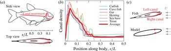
The fish ability to sense minute water motions in their vicinity is attributed to the lateral-line mechanosensory system (Engelmann et al. Reference Engelmann, Hanke, Mogdans and Bleckmann2000). The lateral-line system consists primarily of two types of sensors: superficial and canal neuromasts. Superficial neuromasts are located in the skin and are functionally suited for measuring velocity (Kroese & Schellart Reference Kroese and Schellart1992). Canal neuromasts are recessed in bone-like canals and are thought to measure pressure (Coombs & Van Netten Reference Coombs and Van Netten2005). The layout of the canal sensory system is highly conserved across diverse species and evolutionary time (Coombs, Janssen & Webb Reference Coombs, Janssen and Webb1988); namely, it extends over much of the body but is concentrated near the head (Siregar Reference Siregar1994); see figure 1. This basic arrangement also holds in the blind Mexican cavefish, albeit with more sensory receptors in comparison to their surface-dwelling relatives who retained a functional visual system (Yoshizawa et al. Reference Yoshizawa, Jeffery, Van Netten and McHenry2014).
(a) Spatial distribution of the lateral-line canal neuromasts in Astyanax fasciatus (blind Mexican cave fish), inspired from Montgomery et al. (Reference Montgomery, Coombs and Baker2001). Here,
 $L$
is the total length of the fish and
 $s$
is the arclength measured from the fish head. (b) Canal density in various species of fish, adapted from Ristroph, Liao & Zhang (Reference Ristroph, Liao and Zhang2015). (c) Lateral-line canal in oncoming uniform flow of speed
 $U$
seen from the top and the corresponding model system proposed here.

The universality of the lateral-line architecture suggests a functional advantage in having a higher density of sensors in the anterior segment of the fish. Recent experiments by Ristroph et al. correlate anatomical measurements of canal density with pressure measurements from flow experiments (Ristroph et al. Reference Ristroph, Liao and Zhang2015). They suggest that the relevant sensory output is the difference in pressure between the left and right canals, rather than the absolute pressure itself. They further show that the canal system is concentrated at locations on the body that experience strong variations in this pressure difference. While these findings provide valuable insights into the relevant quantity that is sensed, a deeper understanding of how behaviour emerges from sensory information requires, in addition to identifying the sensory output, knowledge about how such sensory information is processed and translated into decision making and behaviour. It is a complicated task to discern how sensory signals translate into behaviour in live fish. Behaviour is the result of intertwined complex mechanisms, where sensory feedback and neural control, muscular actuation and preflexes, and hydrodynamics are combined to produce the remarkable ability of fish to respond to hydrodynamic cues.
In this work, we propose a mathematically tractable model system that allows us to shed light on some of these questions. Namely, we investigate the optimal sensor placement that maximizes the sensory output, that is, the difference in pressure between the left and right sensors, and how behaviour emerges in light of this sensory information. Our model consists of a planar elliptic body swimming at a constant speed along its major axis, and equipped with pressure sensors located laterally on the two sides of the ellipse in a symmetric configuration about its major axis; see figure 1(c). The sensors provide one sensory output, namely the difference in pressure between the two sides of the body, which is consistent with experimental findings of Ristroph et al. (Reference Ristroph, Liao and Zhang2015). We postulate that the body responds to the sensory output by adjusting its orientation. Our goal is to test whether this hypothesis or ‘control law’ is sufficient to capture the rheotactic behaviour exhibited by many fish species. To this end, we place the fish model in oncoming uniform flows in an otherwise unbounded domain of inviscid and incompressible fluid. We investigate optimal sensor placement in these flows and examine the response of the body to pressure cues. Interestingly, the body responds by aligning with or against the flow, as observed in fish rheotaxis. This rheotactic behaviour depends crucially on the orientation of the fishlike body and its swimming speed relative to the oncoming flow. We conclude by commenting on the relevance of these findings to understanding both the sensory response in fish and the conceptual design of engineered underwater sensory systems.
2 Model
Consider a planar elliptic body with semimajor axis
 $a$
and semiminor axis
 $b$
, submerged in an otherwise unbounded domain of inviscid and incompressible fluid. Let
 $(x_{c},y_{c})$
denote the position of the centre of the body with respect to a fixed inertial frame with Cartesian coordinates
 $(x,y)$
. Let
 ${\it\theta}$
denote the orientation angle measured from the positive
 $x$
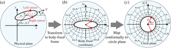
-direction to the major axis of the ellipse, as shown in figure 2(a). The linear and angular velocities of the body are given by
 $({\dot{x}}_{c},{\dot{y}}_{c})$
and
 $\dot{{\it\theta}}$
respectively. Here, the dot
 $(\cdot )$
corresponds to derivative with respect to time
 $t$
. To emulate the fish lateral line, we equip the body with two pressure sensors located at
 $(x_{l},y_{l})$
and
 $(x_{r},y_{r})$
in a symmetric configuration about the major axis of the ellipse. These sensors capture the local value of the pressure field
 $p(x,y)$
to provide one sensory output, namely the difference in pressure
 ${\rm\Delta}p=p(x_{l},y_{l})-p(x_{r},y_{r})$
.
Schematic of the model system (a) in the physical plane, (b) in a body-fixed frame, with dashed lines corresponding to level sets of constant elliptic coordinates, and (c) conformally mapped to the circle plane, with dashed lines corresponding to level sets of constant polar coordinates.

We investigate the dependence of the sensory output
 ${\rm\Delta}p$
on body orientation
 ${\it\theta}$
and swimming velocity
 $V$
in uniform flows of speed
 $U$
in the negative
 $x$
-direction. Analytic expressions for the fluid velocity and pressure fields are obtained by conformally mapping the infinite fluid domain outside the elliptic body into the domain outside a circle of radius
 $R=(a+b)/2$
. For convenience, we introduce the complex coordinate
 $z=x+\text{i}y$
, where
 $\text{i}=\sqrt{-1}$
, in the physical plane, such that the location of the centre of the body is given by
 $z_{c}=x_{c}+\text{i}y_{c}$
and the locations of the sensors are
 $z_{r}=x_{r}+\text{i}y_{r}$
and
 $z_{l}=x_{l}+\text{i}y_{l}$
. These coordinates are then transformed to a body-fixed frame (figure 2
b), prior to mapping the ellipse plane conformally to the circle plane (figure 2
c). The conformal mapping from the circle to the physical plane takes the form (see, e.g., Michelin & Smith (Reference Michelin and Smith2009); Ysasi, Kanso & Newton (Reference Ysasi, Kanso and Newton2011))
 $$\begin{eqnarray}z=z_{c}+\left({\it\zeta}+\frac{{\it\lambda}^{2}}{{\it\zeta}}\right)\text{e}^{\text{i}{\it\theta}}.\end{eqnarray}$$
Here,
 ${\it\zeta}={\it\xi}+\text{i}{\it\eta}$
is the complex variable in the circle plane and
 ${\it\lambda}=(\sqrt{a^{2}-b^{2}})/2$
is a measure of the eccentricity of the ellipse, whereas
 $\text{e}^{(\cdot )}$
denotes the exponential function.
Let
 $u(z)=u_{x}(x,y)+\text{i}u_{y}(x,y)$
denote the complex fluid velocity in the physical plane. The corresponding complex potential function can be written as
 $F(z)={\it\Phi}(x,y)+\text{i}{\it\Psi}(x,y)$
, with
 ${\it\Phi}$
being the real potential function and
 ${\it\Psi}$
the stream function. The existence of
 ${\it\Phi}$
and
 ${\it\Psi}$
is guaranteed by the irrotationality and incompressibility conditions; see, e.g., Lamb (Reference Lamb1932). By linearity of the problem, the complex potential
 $F(z)$
can be written as a superposition of two contributions,
 $F=F_{b}+F_{u}$
, where
 $F_{b}(z)=-V(R^{2}-{\it\lambda}^{2})/{\it\zeta}$
is due to the motion of the elliptic body and
 $F_{u}(z)=-U\text{e}^{\text{i}{\it\theta}}{\it\zeta}-U\text{e}^{-\text{i}{\it\theta}}R^{2}/{\it\zeta}$
is due to the external uniform flow
 $U$
. It should be noted that we neglected the effect of the turning rate
 $\dot{{\it\theta}}$
on
 $F_{b}$
, considering only quasistatic changes in body orientation to best emulate the experimental procedure of Ristroph et al. (Reference Ristroph, Liao and Zhang2015). We introduce non-dimensional counterparts to the above quantities using the characteristic length scale
 ${\it\lambda}$
and time scale
 ${\it\lambda}/U$
. The non-dimensional radius
 $R$
of the circle is given by
 $R=(a+b)/(2{\it\lambda})=\sqrt{(a+b)/(a-b)}$
, and all parameters and variables are now considered in non-dimensional form. To this end, the dimensionless stream function takes the form
 $$\begin{eqnarray}F=F_{b}+F_{u}=V\frac{1-R^{2}}{{\it\zeta}}-{\it\zeta}\text{e}^{\text{i}{\it\theta}}-\frac{R^{2}}{{\it\zeta}}\text{e}^{-\text{i}{\it\theta}}.\end{eqnarray}$$
The complex conjugates
 $\bar{u}({\it\zeta})=u_{{\it\xi}}-\text{i}u_{{\it\eta}}$
and
 $\bar{u}(z)=u_{x}-\text{i}u_{y}$
of the fluid velocity field in the circle and physical planes are given by
 $$\begin{eqnarray}\bar{u}({\it\zeta})=\frac{\text{d}F({\it\zeta})}{\text{d}{\it\zeta}},\quad \bar{u}(z)=\frac{\text{d}F}{\text{d}{\it\zeta}}\frac{\text{d}{\it\zeta}}{\text{d}z}.\end{eqnarray}$$
The pressure field
 $p$
is obtained from the steady Bernoulli equation
 $p-p_{\infty }=-|u|^{2}/2$
, where
 $p_{\infty }$
is the pressure at infinity and is undetermined. The sensory output is given by the difference in pressure between the left and right sensors
 ${\it\zeta}_{l}$
and
 ${\it\zeta}_{r}$
,
 $$\begin{eqnarray}{\rm\Delta}p=p({\it\zeta}_{l})-p({\it\zeta}_{r})={\textstyle \frac{1}{2}}|u|_{{\it\zeta}_{r}}^{2}-{\textstyle \frac{1}{2}}|u|_{{\it\zeta}_{l}}^{2}.\end{eqnarray}$$
The locations of the right and left sensors in the circle plane are expressed as
 ${\it\zeta}_{r}=R\text{e}^{-\text{i}{\it\sigma}}$
and
 ${\it\zeta}_{l}=R\text{e}^{\text{i}{\it\sigma}}$
, with
 ${\it\sigma}$
being the angular position of the sensors (figure 2
c). Alternatively, one could use the arclength
 $s$
normalized by the length
 $L$
, as done in Ristroph et al. (Reference Ristroph, Liao and Zhang2015) (see figure 1
a). In the context of the elliptic model, one can put the normalized arclength
 $s/L$
in one-to-one correspondence with
 ${\it\sigma}$
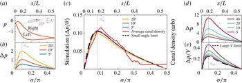
, as noted in figure 3. Hereafter, we use
 ${\it\sigma}$
to refer to the location of the sensors.
(a) Pressure distributions along the body for
 $b/a=0.266$
,
 ${\it\theta}=5^{\circ }$
,
 $V=0$
. (b) Pressure difference
 ${\rm\Delta}p$
in (3.1) as a function of
 ${\it\sigma}$
for
 ${\it\theta}=5^{\circ },10^{\circ }$
and
 $20^{\circ }$
and
 $V=0$
. (c) Stimulation (
 ${\rm\Delta}p/{\it\theta}$
) for
 ${\it\theta}=5^{\circ },10^{\circ }$
and
 $20^{\circ }$
and its theoretical limit obtained by using small
 ${\it\theta}$
in (3.1) compared with the average canal density of figure 1(b). (d) Pressure difference as as a function of
 ${\it\sigma}$
for
 $V=5,10,20,40$
and
 ${\it\theta}=5^{\circ }$
; (e)
 ${\rm\Delta}p/V$
for the same parameter values.

We assume that the fishlike body swims at a constant speed
 $V$
in the direction of its major axis of symmetry (figure 2
a), and responds to sensory information by adjusting its orientation depending on the value of the pressure difference
 ${\rm\Delta}p$
. Namely, we describe the body response to sensory output using the following kinematic model:
 $$\begin{eqnarray}{\dot{x}}_{c}=V\cos {\it\theta},\quad {\dot{y}}_{c}=V\sin {\it\theta},\quad \dot{{\it\theta}}={\it\kappa}{\rm\Delta}p.\end{eqnarray}$$
Here,
 ${\it\kappa}$
is a constant ‘gain’ parameter. The pressure output
 ${\rm\Delta}p$
depends on
 ${\it\theta}$
as well as the location of the pressure sensors
 ${\it\sigma}$
and the swimming speed
 $V$
. Equations (2.5) can be thus viewed as a model of the neuro-mechanic control or response of the fish to sensory information
 ${\rm\Delta}p$
.
3 Results
We first examine the dependence of the sensory output
 ${\rm\Delta}p$
on the location
 ${\it\sigma}$
of the sensors as the body changes orientation relative to the oncoming flow, and we compare our findings with the experimental results of Ristroph et al. (Reference Ristroph, Liao and Zhang2015). One of the advantages of the modelling approach employed here is that it is amenable to analytic expressions for the pressure (expression not shown) and the pressure difference
 ${\rm\Delta}p$
. One gets, upon substituting (2.2) into (2.3) and using the resulting expression in (2.4), that
 $$\begin{eqnarray}{\rm\Delta}p=\frac{2R^{2}\sin (2{\it\sigma})}{R^{4}-2R^{2}\cos (2{\it\sigma})+1}[V(R^{2}-1)\sin ({\it\theta})+R^{2}\sin (2{\it\theta})].\end{eqnarray}$$
It should be noted that the dependence of the function
 ${\rm\Delta}p$
on
 ${\it\sigma}$
is separable from its dependence on
 $V$
and
 ${\it\theta}$
. This property has important consequences on optimal sensor placement, as discussed below.
Figure 3(a) shows the pressure distribution for the right and left sensors as a function of
 ${\it\sigma}$
when the body is oriented at
 ${\it\theta}=10^{\circ }$
. The flow-facing (right) side experiences higher pressure than the leeward (left) side, consistent with Ristroph et al. (Reference Ristroph, Liao and Zhang2015, figure 3). Figure 3(b) depicts
 ${\rm\Delta}p$
as a function of
 ${\it\sigma}$
for three different body orientations,
 ${\it\theta}=5^{\circ },10^{\circ }$
and
 $20^{\circ }$
. The pressure difference increases with increasing
 ${\it\theta}$
, but the dependence on
 ${\it\sigma}$
follows a similar trend for all
 ${\it\theta}$
, which is to be expected from the separability property of
 ${\rm\Delta}p$
in (3.1). The increase in the sensory signal
 ${\rm\Delta}p$
as
 ${\it\theta}$
increases can be interpreted by the swimmer as an indication of the degree of misalignment with the oncoming flow, as noted in Venturelli et al. (Reference Venturelli, Akanyeti, Visentin, Ježov, Chambers, Toming, Brown, Kruusmaa, Megill and Fiorini2012) and Ristroph et al. (Reference Ristroph, Liao and Zhang2015). The qualitative agreement of the results in figure 3(a,b) with the experimental findings in figure 3(a,b) of Ristroph et al. (Reference Ristroph, Liao and Zhang2015) is remarkable (the figures of Ristroph et al. are not reproduced here). To further explore the accord between our model and the experimental results, we plot in figure 3(c) the pressure stimulation parameter, defined in Ristroph et al. as the ratio of the pressure difference to the orientation angle
 ${\rm\Delta}p/{\it\theta}$
. The curves in figure 3(c) collapse into one curve for small
 ${\it\theta}$
, as in Ristroph et al. (Reference Ristroph, Liao and Zhang2015, figure 3). Indeed, for small
 ${\it\theta}$
,
 ${\rm\Delta}p/{\it\theta}$
is independent of
 ${\it\theta}$
, as can be readily verified from (3.1), and, thus, the sensory output
 ${\rm\Delta}p$
scales linearly with
 ${\it\theta}$
. The collapsed curve shows a remarkable resemblance to the average canal density itself, shown in figure 1(b) and overlaid on the stimulation curves in figure 3(d) for direct comparison. This correspondence confirms the findings of Ristroph et al. (Reference Ristroph, Liao and Zhang2015) that the lateral-line canals are concentrated at locations of strong hydrodynamic signals
 ${\rm\Delta}p$
.
We now go beyond the results of Ristroph et al. (Reference Ristroph, Liao and Zhang2015) to explore the effect of the swimming speed
 $V$
on
 ${\rm\Delta}p$
, as shown in figure 3(d) for four different speeds,
 $V=5,10,20$
and 40. Clearly,
 ${\rm\Delta}p$
follows a similar trend for all
 $V$
such that the curves
 ${\rm\Delta}p/V$
(for non-zero
 $V$
) collapse onto one curve for large
 $V$
. The fact that for large
 $V$
,
 ${\rm\Delta}p/V$
is independent of
 $V$
follows immediately from (3.1). It implies that for swimming speeds
 $V$
much larger than the speed of the background flow (here normalized to 1), the sensory output
 ${\rm\Delta}p$
scales linearly with
 $V$
. Further, the value of
 $V$
does not alter the sensor location
 ${\it\sigma}$
for which
 ${\rm\Delta}p$
is maximum. To compute analytically the optimal sensor location
 ${\it\sigma}_{opt}$
for which
 ${\rm\Delta}p$
takes its maximum value, we set
 $\partial {\rm\Delta}p/\partial {\it\sigma}=0$
to find that
 $$\begin{eqnarray}{\it\sigma}_{opt}=\frac{1}{2}\cos ^{-1}\left(\frac{2R^{2}}{R^{4}+1}\right).\end{eqnarray}$$
It follows immediately from the separability property in (2.4) that
 ${\it\sigma}_{opt}$
is independent of
 $V$
and
 ${\it\theta}$
, and depends only on
 $R=\sqrt{(a+b)/(a-b)}$
.
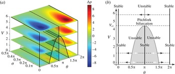
Figure 4(a) is a depiction of the pressure difference
 ${\rm\Delta}p$
as a function of body orientation
 ${\it\theta}$
, swimming speed
 $V$
and sensor location
 ${\it\sigma}$
. This pictorial depiction confirms that the optimal sensor location
 ${\it\sigma}_{opt}$
for which
 ${\rm\Delta}p$
is maximum/minimum is independent of
 $V$
and
 ${\it\theta}$
. Meanwhile, there exist orientations for which the sensory output is identically zero irrespective of sensor placement
 ${\it\sigma}$
. These blind spots, orientations for which the sensory output is zero, are highlighted in black in figure 4(a) and calcuated analytically by setting
 ${\rm\Delta}p=0$
in (3.1) and solving for
 ${\it\theta}$
, which yields
 $$\begin{eqnarray}{\it\theta}^{\ast }=0,\quad {\it\theta}^{\ast }=\cos ^{-1}\left(-V\frac{R^{2}-1}{2R^{2}}\right),\quad {\it\theta}^{\ast }={\rm\pi}(\text{mod}~2{\rm\pi}).\end{eqnarray}$$
That is,
 ${\rm\Delta}p$
is zero for
 ${\it\theta}^{\ast }=0$
and
 ${\rm\pi}$
when the body is aligned opposite to or in the same direction as the oncoming uniform flow. A third blind spot exists only when
 $-1\leqslant -V(R^{2}-1)/2R^{2}\leqslant 1$
, that is, when the swimming speed
 $V$
is below a critical value
 $V_{cr}=2R^{2}/(R^{2}-1)$
.
(a) Pressure difference
 ${\rm\Delta}p$
as a function of body orientation
 ${\it\theta}$
, swimming speed
 $V$
and sensor location
 ${\it\sigma}$
. The black contour lines show
 ${\rm\Delta}p=0$
. (b) The points where
 ${\rm\Delta}p=0$
are fixed points of the governing equations for which the body does not change orientation. The stability of these fixed directions depends on the swimming speed
 $V$
. The ellipse aspect ratio is set to
 $b/a=0.3$
, but the results hold qualitatively for all
 $0<b/a<1$
.

We examine the behaviour when the body changes its orientation in response to the local pressure difference
 ${\rm\Delta}p$
according to (2.5). It should be noted that
 ${\rm\Delta}p$
, and, consequently, the right-hand side of (2.5), depends explicitly on
 ${\it\theta}$
, but not on the position
 $(x_{c},y_{c})$
of the body. This fact is due to the translational symmetry of motion in uniform flows. One can thus ‘reduce’ (2.5) from three equations for
 $(x_{c},y_{c},{\it\theta})$
to one equation in terms of
 ${\it\theta}$
only in the sense that one can solve the orientation equation
 $\dot{{\it\theta}}={\it\kappa}{\rm\Delta}p$
separately. Once the orientation is known, the trajectory in the
 $(x_{c},y_{c})$
plane can be readily reconstructed.
Orientations for which
 ${\rm\Delta}p=0$
are fixed points or, more precisely, relative equilibria of (2.5). Along these directions, the body moves with constant speed
 $V$
without changing orientation. These directions are linearly stable when
 $\partial {\rm\Delta}p/\partial {\it\theta}<0$
and unstable otherwise. A summary of the three families of fixed points and their stability types is given in figure 4(b). For swimmers moving at speeds
 $V<V_{cr}$
, both
 ${\it\theta}^{\ast }=0$
and
 ${\it\theta}^{\ast }={\rm\pi}$
are stable, whereas
 ${\it\theta}^{\ast }=\cos ^{-1}(V/V_{cr})$
is unstable. At
 $V=V_{cr}$
, the system undergoes a subcritical pitchfork bifurcation where the two unstable branches of
 ${\it\theta}^{\ast }=\cos ^{-1}(V/V_{cr})$
collide with the stable branch
 ${\it\theta}^{\ast }={\rm\pi}$
, making it unstable. For
 $V>V_{cr}$
, one has only one stable solution
 ${\it\theta}^{\ast }=0$
where the body aligns in the opposite direction to the oncoming flow. In other words, for low swimming speeds
 $V$
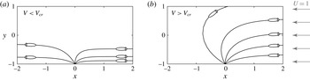
relative to the normalized background flow, the swimmer orients either with or against the flow. As the swimming speed increases, the swimmer orients only in the opposite direction to the flow. Figure 5 depicts representative trajectories for both
 $V<V_{cr}$
and
 $V>V_{cr}$
. These results are consistent with observations of fish rheotaxis, where fish are seen to respond to water motion either by fleeing high-flow regions or by aligning their bodies in the direction opposite to the oncoming flow for upsteam migration and position holding (Arnold Reference Arnold1974; Montgomery, Baker & Carton Reference Montgomery, Baker and Carton1997).
Trajectories of the swimmer in uniform flow for (a)
 $V=1.44$
and (b)
 $V=11.5$
. Initial orientations are
 ${\it\theta}(0)={\rm\pi}/6,{\rm\pi}/3,{\rm\pi}/2,2{\rm\pi}/3,5{\rm\pi}/6$
. Parameter values are
 $b/a=0.3$
,
 $V_{cr}=4.33$
and
 ${\it\kappa}=1$
.

As time increases, the linearly stable direction
 ${\it\theta}^{\ast }=0$
is an attractor for all
 $V$
, and
 ${\it\theta}^{\ast }={\rm\pi}$
is an attractor for
 $V<V_{cr}$
. For each stable direction
 ${\it\theta}^{\ast }$
, the basin of attraction is defined as the set of all initial values of
 ${\it\theta}$
for which the body eventually aligns with
 ${\it\theta}^{\ast }$
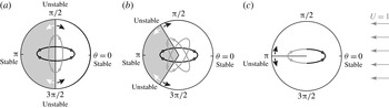
. Figure 6 depicts the basins of attraction for three representative cases corresponding to (a) zero swimming speed
 $V=0$
, (b) swimming at subcritical speeds
 $V<V_{cr}$
and (c) swimming at supercritical speeds
 $V>V_{cr}$
. In (a,b), the set of all orientations is divided into two regions: the white region defines the basin of attraction for the stable orientation
 ${\it\theta}^{\ast }=0$
, where the body aligns in the opposite direction to the flow, and the grey region defines the basin of attraction for
 ${\it\theta}^{\ast }={\rm\pi}$
, for which the body aligns with the flow. For
 $V>V_{cr}$
, the latter orientation becomes unstable and all initial conditions tend to align in the direction opposite to the oncoming flow.
Basins of attraction. (a) For
 $V=0$
, the set of all initial orientations is equally split into a white subset that tends to align in the direction opposite to the incoming flow and a grey subset that tends to align in the same direction as the incoming flow. (b) For
 $0<V<V_{cr}$
, the grey region shrinks until at
 $V=V_{cr}$
a pitchfork bifurcation occurs, making
 ${\it\theta}^{\ast }={\rm\pi}$
unstable. (c) For
 $V>V_{cr}$
, all trajectories, except those parallel to
 ${\rm\pi}$
, tend to align in the direction opposite to the flow.

4 Discussion
The lateral-line sensory system, which contains canal receptors that measure hydrodynamic pressure, is thought to be responsible for the ability of fish to sense minute water motions in their vicinity, and, thus, to play an important role in the fish response to ambient flows, such as fish rheotaxis. Recent findings based on fish anatomical measurements and flow experiments suggest that the arrangement of the lateral-line system is correlated with locations along the fish body that experience strong variations in the hydrodynamic signal (Ristroph et al. Reference Ristroph, Liao and Zhang2015).
In this paper, we presented a mathematical model consisting of an elliptic body equipped with laterally arranged pressure sensors that emulate the fish lateral-line sensory system. We studied the sensory output (the difference in hydrodynamic pressure) in oncoming uniform flows as a function of the sensor location, swimming speed and body orientation. We found that the optimal placement of sensors that maximizes the sensory output is independent of the swimming speed and body orientation, and depends only on the body geometry. Our results are consistent with the experimental findings of Ristroph et al. (Reference Ristroph, Liao and Zhang2015), and support a physical and hydrodynamic explanation of the highly conserved architecture of the lateral-line sensory system across many fish species – the sensory system extends over much of the body but is concentrated near the head. Most fish species have a body plan characterized by high curvature at the head. This body plan leads to a pressure profile that is greatest at the head, making it particularly sensitive to variations in the hydrodynamic signal, such as those due to changes in body orientation or swimming speed.
For small deviations from the oncoming flow direction, the sensory output varies linearly with the body orientation. This linear dependence holds well up to
 ${\it\theta}=20^{\circ }$
. The pressure output also changes linearly with the swimming speed
 $V$
when
 $V$
is much larger than the background flow
 $U=1$
, namely when
 $V/U>40$
. Such linear encoding of changes in sensory signal as the fish swimming parameters change could greatly simplify the neural processing involved in signal decoding. However, this linear dependence does not hold for finite body orientation and relatively moderate swimming speeds, implying that more complex computations are needed to decipher the sensory information in these regimes.
We proposed that the fishlike body responds to these sensory cues by adjusting its orientation proportionally to the perceived difference in pressure. This modelling approach can be viewed as an abstraction, or ‘meta-model’, of the coupling between the sensory output and the neural and muscular drive underlying fish behaviour. Our working hypothesis is that these intertwined sensory, neural and actuation mechanisms produce an emergent rule or law that underlies fish rheotaxis. The behaviour obtained from our proposed model is remarkably similar to fish rheotactic behaviour. At relatively low swimming speeds, fish go with the flow if they are initially oriented in such a way that they cannot hold out against and turn into the oncoming flow. Otherwise, they align into the oncoming flow.
This modelling framework couples the sensory and response mechanisms underlying fish rheotaxis, albeit in the context of a potential flow model. It establishes the response law to sensory signals, regardless of the physiological mechanisms that bring this about. Here, a few comments on the model limitations are in order.
-
(i) We considered a planar model. However, an ellipsoidal body in uniform potential flow leads to similar results on optimal sensor location, equilibrium orientations and stability. In uniform flows, the flow topology and pressure distribution around the centreline of an ellipsoidal body are similar to those around an ellipse – this is the reason why our results agree with the experimental findings of Ristroph et al. (Reference Ristroph, Liao and Zhang2015).
-
(ii) We ignored the effects of viscosity and separation. In the experiments of Ristroph et al. (Reference Ristroph, Liao and Zhang2015), where the fish model is placed in uniform flows, separation occurs at the trailing edge of the fish – thus it does not affect the optimal location of sensors. Viscosity and separation will play prominent roles in non-uniform flows and complex fish manoeuvres. Under these conditions, fish need multiple sensory outputs from their distributed lateral line to decipher the location of flow separation.
-
(iii) The control law in (2.5) is linear. This is in part due to the lack of experimental evidence to support a particular choice of linear versus nonlinear control law. More importantly, a linear control law simplifies the neural processing involved in responding to a given sensory output. Therefore, it is reasonable to conjecture that a linear law is preferable. We showed that the linear model leads the proper rheotactic behaviour. More complex fish behaviour might require more complex control laws.
-
(iv) The model in (2.5) is kinematic. That is to say, it does not explicitly account for forces and moments, although they can be calculated posteriori for each trajectory using balance of momenta. Kinematic models are common in studying emergent behaviour such as in fish schooling (Couzin et al. Reference Couzin, Krause, James, Ruxton and Franks2002), where details of the coupling among the sensory feedback, neural control and muscular actuation are not fully understood. Our goal here was to test whether the rule ‘turn in response to sensory output’ reproduces fishlike rheotaxis. We will link this rule-based model to the mechanics of motion in ambient flows in future studies.
The two main results obtained from the simplified model – the optimal sensor placement that maximizes the sensory output and how rheotactic behaviour emerges in light of this sensory information – serve to direct future research. We focused here on single sensory output and rheotactic behaviour in uniform flows. However, future work will address the interplay of multiple sensory outputs and how such sensory information could be used to avoid collision with nearby objects, detect ambient vorticity and inform changes in the fish body undulations (Fernandez et al. Reference Fernandez, Maertens, Yaul, Dahl, Lang and Triantafyllou2011; Ren & Mohseni Reference Ren and Mohseni2012; Yanase, Herbert & Montgomery Reference Yanase, Herbert and Montgomery2012). Future models will also account for three-dimensional and viscous effects (Hassan Reference Hassan1992; Eldredge Reference Eldredge2008; Gazzola et al. Reference Gazzola, Chatelain, van Rees and Koumoutsakos2011), which we expect to play a prominent role in non-planar fish motions and manoeuvres as well as in non-uniform and high-speed flows, where flow separation is paramount. These models could also serve as a design tool for developing optimal sensory layouts and deployment strategies of underwater vehicles (Yang et al. Reference Yang, Chen, Engel, Pandya, Chen, Tucker, Coombs, Jones and Liu2006; Fernandez et al. Reference Fernandez, Maertens, Yaul, Dahl, Lang and Triantafyllou2011; Venturelli et al. Reference Venturelli, Akanyeti, Visentin, Ježov, Chambers, Toming, Brown, Kruusmaa, Megill and Fiorini2012; Triantafyllou, Weymouth & Miao Reference Triantafyllou, Weymouth and Miao2016). The development of autonomous vehicles that detect hydrodynamic cues is important for their deployment in unknown underwater environments, and is relevant for many environmental, military and industrial applications, including ocean exploration, navigation, surveillance and monitoring.
Acknowledgements
This work is partially supported by the ONR grant 14-001. B.C. acknowledges the support of the Department of Defense (DoD) through a National Defense Science and Engineering Graduate (NDSEG) Fellowship.