1 Introduction
Electrical actuation of drops and bubbles provides a useful means of manipulating their motion and shape deformation in a controllable fashion inside microfluidic environments. Such manipulation techniques have found emerging applications in the fields of atomization (Wu & Clark Reference Wu and Clark2008), enhanced mixing of reagents (Hoburg & Melcher Reference Hoburg and Melcher1977; Tsouris et al. Reference Tsouris, Culbertson, DePaoli, Jacobson, De Almeida and Ramsey2003), enhanced coalescence and separation (Ptasinski & Kerkhof Reference Ptasinski and Kerkhof1992), ink-jet printing (Basaran Reference Basaran2002) etc. Adding to this, various nonlinear phenomena such as the shape deformation (Taylor Reference Taylor1966; Haber & Hetsroni Reference Haber and Hetsroni1971), fluid inertia (Mortazavi & Tryggvason Reference Mortazavi and Tryggvason2000; Magnaudet Reference Magnaudet2003), viscoelasticity (Mukherjee & Sarkar Reference Mukherjee and Sarkar2013) and the presence of surface-active agents (Baret Reference Baret2012; Anna Reference Anna2016) typically interact with the drop dynamics either being intentionally introduced or present in the system owing to unavoidable physical circumstances.
Pressure-driven flow offers a common means of manipulating droplets in fluidic confinements. It has been observed previously, that a drop migrates across the flow direction if there is a gradient in the shear stress of the applied flow field, which is typical for Poiseuille flow (Haber & Hetsroni Reference Haber and Hetsroni1971; Chan & Leal Reference Chan and Leal1979). The gradients in the incipient flow field, coupled with various nonlinear effects, greatly influence the drop movement even in the creeping flow limit (Chan & Leal Reference Chan and Leal1979; Mortazavi & Tryggvason Reference Mortazavi and Tryggvason2000; Stan et al. Reference Stan, Guglielmini, Ellerbee, Caviezel, Stone and Whitesides2011). The situation becomes further involved, when an external electric field is present (Chakraborty & Mittal Reference Chakraborty and Mittal2007; Bhaumik et al. Reference Bhaumik, Das, Chakraborty and Dasgupta2014; Dey et al. Reference Dey, Ghosh, Chakraborty and Dasgupta2015). Under such circumstances, the surface charges on the drop give rise to a net interfacial electrostatic stress known as the Maxwell stress. Interfacial charge convection, in turn, plays an important role in modifying the electrohydrodynamic flow pattern and the shape deformation (Saville Reference Saville1997; Feng Reference Feng1999; Xu et al. Reference Xu, Li, Lowengrub and Zhao2006; Lanauze, Walker & Khair Reference Lanauze, Walker and Khair2015; Yariv & Almog Reference Yariv and Almog2016; Sengupta, Walker & Khair Reference Sengupta, Walker and Khair2017) of the droplet. As a consequence, cross-stream migration of the droplet becomes possible (Mandal, Bandopadhyay & Chakraborty Reference Mandal, Bandopadhyay and Chakraborty2016c ).
Owing to their abilities in modifying the interfacial properties of the drops, the nonlinear effects of surfactants have proven to be immensely useful in diverse applications such as emulsion stabilization, drop generation and many others (Fischer & Erni Reference Fischer and Erni2007; Baroud, Gallaire & Dangla Reference Baroud, Gallaire and Dangla2010). The underlying theoretical foundations have been premised on spherical (Pak, Feng & Stone Reference Pak, Feng and Stone2014; Hanna & Vlahovska Reference Hanna and Vlahovska2010) as well as deformable drops (Das, Mandal & Chakraborty Reference Das, Mandal and Chakraborty2017a ; Panigrahi, Das & Chakraborty Reference Panigrahi, Das and Chakraborty2018). The impact of the surfactant-induced Marangoni effects in modifying the electrohydrodynamic flow and subsequent drop deformation and breakup was explored through experiments reported by Ha & Yang (Reference Ha and Yang1998) and Zhang et al. (Reference Zhang, He, Ghadiri and Hassanpour2015). These observations have been explained in light of relevant theory within the axisymmetric paradigm (Ha & Yang Reference Ha and Yang1995; Teigen & Munkejord Reference Teigen and Munkejord2010; Nganguia et al. Reference Nganguia, Young, Vlahovska, Bławzdziewcz, Zhang and Lin2013; Mandal, Bandopadhyay & Chakraborty Reference Mandal, Bandopadhyay and Chakraborty2016a ; Poddar et al. Reference Poddar, Mandal, Bandopadhyay and Chakraborty2018).
Can one switch the cross-stream migration of electrically modulated droplets in a Poiseuille flow at will? Here, we demonstrate, through a comprehensive three-dimensional analytical approach, that the same is indeed a possibility by exploiting a non-trivial interplay of viscous, Marangoni and electrical stresses at the drop–carrier interface. Ingenuity of the physics addressed in the present problem stems from the fact that the Marangoni stress itself is a function of surfactant concentration at the interface, which depends on the drop surface velocity. This, in turn, alters the surface charge convection, and hence modulates the (electrical Maxwell) stress at the interface. In an effort to realize a tangential force balance at the interface, the hydrodynamic stress accordingly alters, leading to a modification in the surface velocity. As a consequence, the Marangoni stresses and electrical stresses tend to vary. This, in effect, represents a complex and inter-connected nonlinear coupling of the variable surface tension, charge distribution and shape deformation underlying effects, so that their resultant may not be realized as an effective linear superposition of the individual implications acting in tandem, despite operating in a low Reynolds number regime. Our results can be of profound importance in achieving deep insight into the physical mechanisms towards an additional degree of control of drop motion in microfluidic environments.
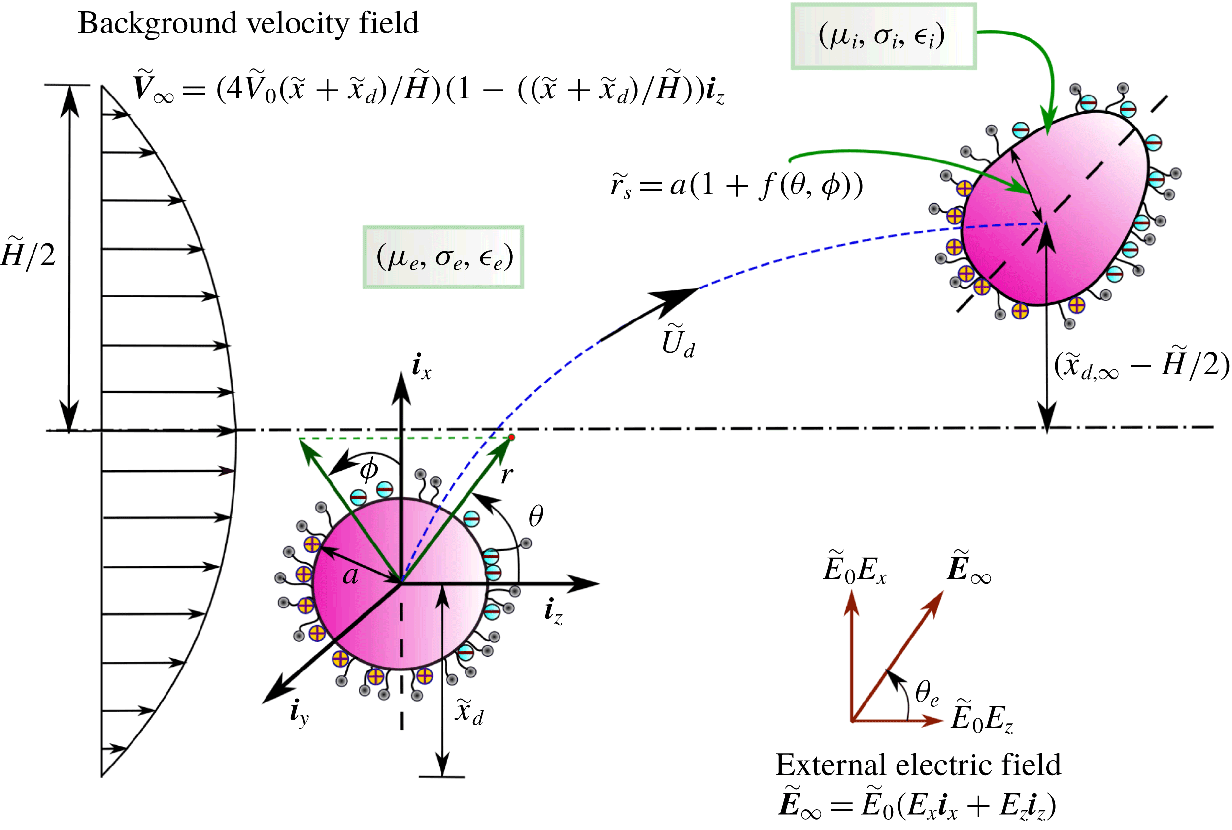
Schematic of a viscous, deformable and surfactant-covered drop which is simultaneously acted upon by background plane Poiseuille flow
 $(\widetilde{\boldsymbol{V}}_{\infty })$
and a tilted electric field
 $\widetilde{\boldsymbol{E}}_{\infty }$
(with a tilt angle
 $\unicode[STIX]{x1D703}_{e}$
). A non-uniform accumulation of charge on the drop interface is also shown. A three-dimensional coordinate system (
 $\widetilde{r},\unicode[STIX]{x1D703},\unicode[STIX]{x1D719}$
) is fitted at the centroid of the moving drop. The drop can translate in the plane of the imposed fields with a constant velocity,
 $\widetilde{\boldsymbol{U}}_{d}=\widetilde{V}_{0}(U_{d,x}\boldsymbol{i}_{x}+U_{d,y}\boldsymbol{i}_{y}+U_{d,z}\boldsymbol{i}_{z})$
. The initial transverse position of the drop from the channel bottom plane is denoted by
 $\widetilde{x}_{d}$
while its final steady-state position is given by
 $\widetilde{x}_{d,\infty }$
.

2 Problem formulation
2.1 Description of the physical system
In the present study we consider a viscous drop of radius
 $a$
migrating through another viscous medium which obeys a plane Poiseuille flow. We consider a pressure-driven flow in the
 $z$
-direction between two infinite-width flat plates which are kept at a distance
 $\widetilde{H}$
apart as shown in figure 1. Thus the imposed flow profile can be mathematically denoted by
 $$\begin{eqnarray}\widetilde{\boldsymbol{V}}_{\infty }=\widetilde{V}_{0}\biggl(c_{0}+c_{1}\left({\displaystyle \frac{\widetilde{x}}{a}}\right)+c_{2}\left({\displaystyle \frac{\widetilde{x}}{a}}\right)^{2}\biggr)\boldsymbol{i}_{z},\end{eqnarray}$$
where
 $$\begin{eqnarray}c_{0}={\displaystyle \frac{4\,\widetilde{x}_{d}}{\widetilde{H}}}\left(1-{\displaystyle \frac{\widetilde{x}_{d}}{\widetilde{H}}}\right),\quad c_{1}={\displaystyle \frac{4\,a}{\widetilde{H}}}\left(1-{\displaystyle \frac{2\widetilde{x}_{d}}{\widetilde{H}}}\right),\quad c_{2}=-{\displaystyle \frac{4\,a^{2}}{\widetilde{H}^{2}}}\end{eqnarray}$$
and
 $\widetilde{V}_{0}$
is the fluid velocity at the channel centreline. The channel height
 $\widetilde{H}$
is considered to be much larger than the drop diameter. If an instant of time the drop is at a distance
 $\widetilde{x}_{d}$
apart from the bottom plate then from the fixed reference frame the imposed flow profile can be alternatively written as
 $$\begin{eqnarray}\boldsymbol{V}_{\infty }={\displaystyle \frac{4\widetilde{V}_{0}(\widetilde{x}+\widetilde{x}_{d})}{\widetilde{H}}}\left(1-{\displaystyle \frac{\widetilde{x}+\widetilde{x}_{d}}{\widetilde{H}}}\right)\boldsymbol{i}_{z}.\end{eqnarray}$$
The drop is simultaneously acted upon by an imposed DC electric field
 $\widetilde{\mathbf{E}}_{\infty }=\widetilde{E}_{0}(E_{x}\boldsymbol{i}_{x}+E_{z}\boldsymbol{i}_{z})$
in the
 $xz$
plane, where
 $\widetilde{E}_{0}$
is the chosen characteristic electric field strength and the Cartesian components are related as
 $\sqrt{E_{x}^{2}+E_{z}^{2}}=1$
. The physical configuration of the present problem prohibits us from adopting a simplified axisymmetric coordinate system. Hence we employ a full three-dimensional coordinate system capable of capturing the possible variations of the variables in all three spatial directions. The drop surface is considered to be contaminated with non-ionic surfactant molecules with a concentration distribution
 $\widetilde{\unicode[STIX]{x1D6E4}}(\unicode[STIX]{x1D703},\unicode[STIX]{x1D719})$
. This non-uniform distribution of surfactant molecules modifies the interfacial tension of the drop given by
 $\widetilde{\unicode[STIX]{x1D6FE}}(\unicode[STIX]{x1D703},\unicode[STIX]{x1D719})$
. Since the drop surface can deform, it assumes a shape with varying contour
 $r_{S}(\unicode[STIX]{x1D703},\unicode[STIX]{x1D719})$
while migrating in the cross-stream as well as far downstream along the channel.
2.2 Governing equations and boundary conditions
2.2.1 Non-dimensionalization scheme
In order to identify the various important dimensionless numbers and property ratios we choose the drop radius
 $a$
as a reference length scale, the centreline velocity of the plane Poiseuille flow
 $\widetilde{V}_{0}$
as reference velocity scale and equilibrium surfactant concentration
 $\widetilde{\unicode[STIX]{x1D6E4}}_{eq}$
as surfactant concentration scale. In addition to that we choose the physical quantities of the surrounding fluid such as viscosity
 $(\unicode[STIX]{x1D707}_{e})$
, dielectric permittivity
 $(\unicode[STIX]{x1D716}_{e})$
and electrical conductivity
 $(\unicode[STIX]{x1D70E}_{e})$
as references for property values. As a consequence of the above non-dimensionalization scheme the following important dimensionless parameters appear in the analysis.
(i) The relative importance between electric stress (
 ${\sim}\unicode[STIX]{x1D716}_{e}E_{0}^{2}$
) and hydrodynamic stress (
${\sim}\unicode[STIX]{x1D707}_{e}\widetilde{V}_{0}/a$
) is depicted by the Mason number, (2.4)$$\begin{eqnarray}M=\unicode[STIX]{x1D716}_{e}aE_{0}^{2}/\unicode[STIX]{x1D707}_{e}\widetilde{V}_{0}.\end{eqnarray}$$
(ii) The deformable nature of drop shape is quantified by the capillary number,
(2.5)which signifies the relative strength of viscous and capillary stresses.$$\begin{eqnarray}Ca=\unicode[STIX]{x1D707}_{e}\widetilde{V}_{0}/\widetilde{\unicode[STIX]{x1D6FE}}_{eq},\end{eqnarray}$$
(iii) The ratio between two important time scales associated with the electric charge, namely the charge relaxation time scale
$t_{cr}=\unicode[STIX]{x1D716}_{e}/\unicode[STIX]{x1D70E}_{e}$
and the charge convection time scale
$t_{cc}=a/\widetilde{V}_{0}$
, is denoted by electric Reynolds number (2.6)$$\begin{eqnarray}Re_{E}=\unicode[STIX]{x1D716}_{e}\widetilde{V}_{0}/a\unicode[STIX]{x1D70E}_{e}.\end{eqnarray}$$
(iv) The surface Péclet number
(2.7)which stands for the relative strength of surface convection and surface diffusion at the drop surface.$$\begin{eqnarray}Pe=a\,\widetilde{V}_{0}/D_{\!_{S}},\end{eqnarray}$$
(v) Electrical permittivity ratio between drop phase and continuous medium,
(2.8)$$\begin{eqnarray}S=\unicode[STIX]{x1D716}_{i}/\unicode[STIX]{x1D716}_{e}.\end{eqnarray}$$
(vi) Electrical conductivity ratio between drop phase and continuous medium,
(2.9)$$\begin{eqnarray}R=\unicode[STIX]{x1D70E}_{i}/\unicode[STIX]{x1D70E}_{e}.\end{eqnarray}$$
(vii) Viscosity ratio between drop phase and continuous medium,
(2.10)$$\begin{eqnarray}\unicode[STIX]{x1D706}=\unicode[STIX]{x1D707}_{i}/\unicode[STIX]{x1D707}_{e}.\end{eqnarray}$$


Henceforth all the
 $\widetilde{\,\,}$
symbols will be dropped to denote the non-dimensional forms of the field variables and property ratios.
2.2.2 Surfactant transport
Under the assumption of bulk insolubility of surfactant, the local concentration distribution of surfactant molecules on the drop surface is dictated by a competition between diffusion and advection processes. In general the governing equation for surfactant transport takes a form (Stone & Leal Reference Stone and Leal1990; Li & Pozrikidis Reference Li and Pozrikidis1997; Leal Reference Leal2007)
 $$\begin{eqnarray}Pe\unicode[STIX]{x1D735}_{S}\boldsymbol{\cdot }(\boldsymbol{u}_{\!_{\,S}}\unicode[STIX]{x1D6E4})=\unicode[STIX]{x1D6FB}_{\!_{S}}^{2}\unicode[STIX]{x1D6E4}.\end{eqnarray}$$
In the above equation
 $\unicode[STIX]{x1D735}_{\!_{S}}$
is the surface divergence operator defined as
 $\unicode[STIX]{x1D735}_{\!_{S}}=(\boldsymbol{I}-\boldsymbol{n}\boldsymbol{n})\boldsymbol{\cdot }\unicode[STIX]{x1D735}$
where
 $\boldsymbol{n}$
denotes the unit normal vector at the drop surface and
 $\boldsymbol{u}_{S}$
is the fluid velocity at the surface of the drop. The surfactant concentration also adheres to a mass conservation at the drop surface denoted as
 $$\begin{eqnarray}\int _{\unicode[STIX]{x1D719}=0}^{2\unicode[STIX]{x03C0}}\int _{\unicode[STIX]{x1D703}=0}^{\unicode[STIX]{x03C0}}\unicode[STIX]{x1D6E4}(\unicode[STIX]{x1D703},\unicode[STIX]{x1D719})\,r_{\!_{S}}^{2}(\unicode[STIX]{x1D703},\unicode[STIX]{x1D719})\sin \unicode[STIX]{x1D703}\,\text{d}\unicode[STIX]{x1D703}\,\text{d}\unicode[STIX]{x1D719}=4\unicode[STIX]{x03C0}.\end{eqnarray}$$
Here we assume a dilute concentration of surfactant and a small deviation from the equilibrium throughout the system. This allows us to consider a linearized version of the equation of state given as (Stone & Leal Reference Stone and Leal1990; Li & Pozrikidis Reference Li and Pozrikidis1997)
 $$\begin{eqnarray}\widetilde{\unicode[STIX]{x1D6FE}}(\widetilde{\unicode[STIX]{x1D6E4}})=\widetilde{\unicode[STIX]{x1D6FE}}_{c}-R_{g}T\,\widetilde{\unicode[STIX]{x1D6E4}},\end{eqnarray}$$
where
 $R_{g}$
is the ideal gas constant,
 $T$
is the absolute temperature and
 $\widetilde{\unicode[STIX]{x1D6FE}}_{c}$
is the surface tension of a surfactant-free drop which are related mutually by
 $\widetilde{\unicode[STIX]{x1D6FE}}_{eq}=\widetilde{\unicode[STIX]{x1D6FE}}_{c}-R_{g}T\,\widetilde{\unicode[STIX]{x1D6E4}}_{eq}$
. Under these considerations (2.13) becomes
 $$\begin{eqnarray}\widetilde{\unicode[STIX]{x1D6FE}}(\widetilde{\unicode[STIX]{x1D6E4}})=\widetilde{\unicode[STIX]{x1D6FE}}_{eq}+R_{g}T(\widetilde{\unicode[STIX]{x1D6E4}}_{eq}-\widetilde{\unicode[STIX]{x1D6E4}}).\end{eqnarray}$$
2.2.3 Electrostatic problem
Following the Taylor–Melcher leaky dielectric model (Melcher & Taylor Reference Melcher and Taylor1969; Saville Reference Saville1997), in the present study we have considered an absence of volumetric charges and only surface accumulation of charge is taken into account. Thus electric potentials in and around the drop (
 $\unicode[STIX]{x1D711}_{i},\unicode[STIX]{x1D711}_{e}$
) are governed by the Laplace equations, given as
 $$\begin{eqnarray}\unicode[STIX]{x1D6FB}^{2}\unicode[STIX]{x1D711}_{i,e}=0.\end{eqnarray}$$
The electric potential takes finite values inside the drop, i.e.
 $\unicode[STIX]{x1D711}_{i}$
is bounded at
 $r\leqslant r_{S}$
. Also the far-stream potential gradient is determined by the imposed electric field by the following relation: as
 $r\rightarrow \infty ,$
 $\unicode[STIX]{x1D735}\unicode[STIX]{x1D711}_{e}=-\boldsymbol{E}_{\infty }$
. At the drop interface potential continuity is satisfied. The interface balance of charges is governed by a competition between ohmic conduction and surface convection of accumulation charges. In addition we consider the approximation of quasi-steady state which assumes instantaneous adjustment of surface charges to the background flow field. Thus in mathematical notation the charge balance at the interface becomes
 $$\begin{eqnarray}\text{at }r=r_{\!_{S}}(\unicode[STIX]{x1D703},\unicode[STIX]{x1D719})\quad \boldsymbol{n}\boldsymbol{\cdot }(R\unicode[STIX]{x1D735}\unicode[STIX]{x1D711}_{i}-\unicode[STIX]{x1D735}\unicode[STIX]{x1D711}_{e})=-Re_{E}\unicode[STIX]{x1D735}_{\!_{S}}\boldsymbol{\cdot }(q\,_{\!_{S}}\boldsymbol{u}_{\,\!_{S}}).\end{eqnarray}$$
The interfacial charge density (
 $q_{\!_{\,S}}$
) appearing in (2.16) is caused by a mismatch between the electrical properties of the two fluids and is determined by the relation
 $$\begin{eqnarray}q_{\!_{\,S}}(\unicode[STIX]{x1D703},\unicode[STIX]{x1D719})=\boldsymbol{n}\boldsymbol{\cdot }(S\unicode[STIX]{x1D735}\unicode[STIX]{x1D711}_{i}-\unicode[STIX]{x1D735}\unicode[STIX]{x1D711}_{e})\big|_{r=r_{\!_{S}}}^{}.\end{eqnarray}$$
The influence of fluid flow on the electric potential distribution is embedded in (2.16), hence suggesting a two-way coupled nature of the electrostatics and hydrodynamics in the present problem.
2.2.4 Hydrodynamic problem
Here we assume the creeping flow limit
 $(Re\ll 1)$
(Happel & Brenner Reference Happel and Brenner1981) for flow inside and outside of the drop and thus neglect the inertia term in the Navier–Stokes equation. Thus the hydrodynamics can be fully described by the Stokes-flow equations and the incompressibility conditions given as
 $$\begin{eqnarray}\left.\begin{array}{@{}c@{}}-\unicode[STIX]{x1D735}p_{i}+\unicode[STIX]{x1D706}\unicode[STIX]{x1D6FB}^{2}\boldsymbol{u}_{i}=0,\quad \unicode[STIX]{x1D735}\boldsymbol{\cdot }\boldsymbol{u}_{i}=0,\\ -\unicode[STIX]{x1D735}p_{e}+\unicode[STIX]{x1D6FB}^{2}\boldsymbol{u}_{e}=0,\quad \unicode[STIX]{x1D735}\boldsymbol{\cdot }\boldsymbol{u}_{e}=0.\end{array}\right\}\end{eqnarray}$$
The velocity and pressure inside the drop (
 $\boldsymbol{u}_{\!\,_{i}},p_{\!\,_{i}}$
) satisfy boundedness at the origin of the reference frame which is fitted at the drop centroid and translates with the drop
 $(\boldsymbol{U}_{d})$
. In the far field, flow velocity approaches the imposed plane Poiseuille flow condition, i.e. at
 $r\rightarrow \infty ,\boldsymbol{u}_{e}=\boldsymbol{V}_{\infty }-\boldsymbol{U}_{d}$
. At the drop interface fluid velocities are continuous
 $(\boldsymbol{u}_{i}=\boldsymbol{u}_{e})$
and follow a quasi-steady-state no-penetration condition
 $(\boldsymbol{u}_{i}\boldsymbol{\cdot }\boldsymbol{n}=\boldsymbol{u}_{e}\boldsymbol{\cdot }\boldsymbol{n}=0)$
.
For a clean drop the hydrodynamic and electric stresses balance each other at the interface. However when the drop surface is coated with a non-uniform distribution of surfactants, an additional interface stress component known as the Marangoni stress, contributes to this balance. Thus the resultant stress balance takes the following form:
 $$\begin{eqnarray}\displaystyle \text{at }r & = & \displaystyle r_{\!_{S}}(\unicode[STIX]{x1D703},\unicode[STIX]{x1D719}),\quad (\unicode[STIX]{x1D749}_{e}^{H}+M\,\unicode[STIX]{x1D749}_{e}^{E})\boldsymbol{\cdot }\boldsymbol{n}-(\unicode[STIX]{x1D749}_{i}^{H}+M\,\unicode[STIX]{x1D749}_{i}^{E})\boldsymbol{\cdot }\boldsymbol{n}\nonumber\\ \displaystyle & = & \displaystyle {\displaystyle \frac{1}{Ca}}(\unicode[STIX]{x1D735}\boldsymbol{\cdot }\boldsymbol{n})\boldsymbol{n}+\underbrace{Ma\,[(1-\unicode[STIX]{x1D6E4})(\unicode[STIX]{x1D735}\boldsymbol{\cdot }\boldsymbol{n})\boldsymbol{n}+\unicode[STIX]{x1D735}_{\!_{S}}\unicode[STIX]{x1D6E4}]}_{Marangoni~stress},\end{eqnarray}$$
where
 $Ma$
denotes the Marangoni number defined as
 $Ma=R_{g}T\,\widetilde{\unicode[STIX]{x1D6E4}}_{eq}/\unicode[STIX]{x1D707}_{e}\widetilde{V}_{0}$
signifying the ratio between the characteristic Marangoni stress and viscous stress. The viscous stress tensors
 $(\unicode[STIX]{x1D749}_{i}^{H},\unicode[STIX]{x1D749}_{e}^{H})$
and electric stress tensors
 $(\unicode[STIX]{x1D749}_{i}^{E},\unicode[STIX]{x1D749}_{e}^{E})$
are defined as
 $$\begin{eqnarray}\left.\begin{array}{@{}c@{}}\,\unicode[STIX]{x1D749}_{i}^{H}=-p_{i}\boldsymbol{ I}+\unicode[STIX]{x1D706}[\unicode[STIX]{x1D735}\boldsymbol{u}_{i}+(\unicode[STIX]{x1D735}\boldsymbol{u}_{i})^{\text{T}}]\\ \unicode[STIX]{x1D749}_{e}^{H}=-p_{e}\boldsymbol{I}+[\unicode[STIX]{x1D735}\boldsymbol{u}_{e}+(\unicode[STIX]{x1D735}\boldsymbol{u}_{e})^{\text{T}}]\end{array}\right\}\quad \text{and}\quad \left.\begin{array}{@{}c@{}}\,\,\,\unicode[STIX]{x1D749}_{i}^{E}=S\left[\boldsymbol{E}_{i}\boldsymbol{E}_{i}^{\text{T}}-{\textstyle \frac{1}{2}}|\boldsymbol{E}_{i}|^{2}\boldsymbol{I}\right]\\ \unicode[STIX]{x1D749}_{e}^{E}=\left[\boldsymbol{E}_{e}\boldsymbol{E}_{e}^{\text{T}}-{\textstyle \frac{1}{2}}\left|\boldsymbol{E}_{e}\right|^{2}\boldsymbol{I}\right]\end{array}\right\}.\end{eqnarray}$$
The non-uniformity in surfactant concentration on the surface is characterized by the elasticity number
 $\unicode[STIX]{x1D6FD}(0\leqslant \unicode[STIX]{x1D6FD}\leqslant 1)$
(Stone & Leal Reference Stone and Leal1990; Li & Pozrikidis Reference Li and Pozrikidis1997; Mandal et al.
Reference Mandal, Bandopadhyay and Chakraborty2016a
) which is defined as
 $$\begin{eqnarray}\unicode[STIX]{x1D6FD}=-{\displaystyle \frac{\widetilde{\unicode[STIX]{x1D6E4}}_{eq}}{\widetilde{\unicode[STIX]{x1D6FE}}_{c}}}{\displaystyle \frac{\text{d}\widetilde{\unicode[STIX]{x1D6FE}}}{\text{d}\widetilde{\unicode[STIX]{x1D6E4}}}}.\end{eqnarray}$$
Here the surface elasticity number
 $(\unicode[STIX]{x1D6FD})$
is varied between a range of 0 and 0.8. While some the investigators (Eggleton, Pawar & Stebe Reference Eggleton, Pawar and Stebe1999; Teigen & Munkejord Reference Teigen and Munkejord2010) have doubted such a range of
 $\unicode[STIX]{x1D6FD}$
owing to the linear relationship between the interface tension and surface concentration (2.14), Li & Pozrikidis (Reference Li and Pozrikidis1997) in their detailed numerical simulations found that such a range closely predicts the actual behaviour in many situations. The influence of surfactant concentration may thus be seen in the tangential and normal stress balances as
 $$\begin{eqnarray}\displaystyle \displaystyle \text{at }\,r=r_{\!_{S}}(\unicode[STIX]{x1D703},\unicode[STIX]{x1D719}),\quad & & \displaystyle \displaystyle \left[(\unicode[STIX]{x1D749}_{e}^{H}+M\,\unicode[STIX]{x1D749}_{e}^{E})\boldsymbol{\cdot }\boldsymbol{n}-(\unicode[STIX]{x1D749}_{i}^{H}+M\,\unicode[STIX]{x1D749}_{i}^{E})\boldsymbol{\cdot }\boldsymbol{n}\right]\boldsymbol{\cdot }(\boldsymbol{I}-\boldsymbol{n}\boldsymbol{n})\nonumber\\ \displaystyle & & \displaystyle \hspace{26.39996pt}=\displaystyle \underbrace{{\displaystyle \frac{\unicode[STIX]{x1D6FD}}{Ca(1-\unicode[STIX]{x1D6FD})}}\,(\unicode[STIX]{x1D735}_{\!_{S}}\unicode[STIX]{x1D6E4})\boldsymbol{\cdot }(\boldsymbol{I}-\boldsymbol{n}\boldsymbol{n})}_{Marangoni~effect}\end{eqnarray}$$
and
 $$\begin{eqnarray}\displaystyle \displaystyle \text{at }\,r=r_{\!_{S}}(\unicode[STIX]{x1D703},\unicode[STIX]{x1D719}),\quad & & \displaystyle \displaystyle \left[(\unicode[STIX]{x1D749}_{e}^{H}+M\,\unicode[STIX]{x1D749}_{e}^{E})\boldsymbol{\cdot }\boldsymbol{n}-(\unicode[STIX]{x1D749}_{i}^{H}+M\,\unicode[STIX]{x1D749}_{i}^{E})\boldsymbol{\cdot }\boldsymbol{n}\right]\boldsymbol{\cdot }\boldsymbol{n}\nonumber\\ \displaystyle & & \displaystyle \hspace{26.39996pt}=\displaystyle {\displaystyle \frac{1}{Ca}}(\unicode[STIX]{x1D735}\boldsymbol{\cdot }\boldsymbol{n})+\underbrace{{\displaystyle \frac{\unicode[STIX]{x1D6FD}}{Ca(1-\unicode[STIX]{x1D6FD})}}\,[(1-\unicode[STIX]{x1D6E4})(\unicode[STIX]{x1D735}\boldsymbol{\cdot }\boldsymbol{n})]}_{Marangoni~effect},\end{eqnarray}$$
respectively. Here
 $(\boldsymbol{I}-\boldsymbol{n}\boldsymbol{n})$
is the surface projection operator.
2.3 Solution using asymptotic perturbation
We proceed by considering a feasible range of the dimensionless parameters involved. In most of the practical conditions these parameters are found to be in the range:
 $Ca\ll 1,Re_{E}\ll 1\text{ and }M\sim 1$
(Xu & Homsy Reference Xu and Homsy2006; Mhatre & Thaokar Reference Mhatre and Thaokar2013; Bandopadhyay et al.
Reference Bandopadhyay, Mandal, Kishore and Chakraborty2016). Hence we choose
 $Ca$
and
 $Re_{E}$
as perturbation parameters and proceed to obtain a solution using a double asymptotic perturbation.
It is important to note that a perturbation scheme based on the surface Péclet number
 $(Pe)$
has been previously employed in several earlier studies (Subramanian & Balasubramaniam Reference Subramanian and Balasubramaniam2005; Pak et al.
Reference Pak, Feng and Stone2014; Das et al.
Reference Das, Mandal and Chakraborty2017a
) related to spherical drop surfaces. In the present consideration of a deformable drop surface it is not possible to adopt
 $Ca$
and
 $Pe$
as independent dimensionless numbers (Stone & Leal Reference Stone and Leal1990; Mandal et al.
Reference Mandal, Bandopadhyay and Chakraborty2016a
). Thus we take a different route and define a dimensionless physicochemical parameter composed of different property constants and the length scale as (Stone & Leal Reference Stone and Leal1990; Mandal et al.
Reference Mandal, Bandopadhyay and Chakraborty2016a
; Das et al.
Reference Das, Mandal and Chakraborty2017a
)
 $$\begin{eqnarray}k={\displaystyle \frac{Pe}{Ca}}={\displaystyle \frac{\widetilde{\unicode[STIX]{x1D6FE}}_{eq}\,a}{\unicode[STIX]{x1D707}_{e}\,D_{\!_{S}}}}.\end{eqnarray}$$
We can now express the Péclet number in terms of
 $k$
and
 $Ca$
as
 $(Pe=k\,Ca)$
. Based on the values of relevant dimensional physical quantities two different regimes can be classified for the surfactant transport: (i) diffusion dominated regime or the low surface Péclet limit (
 $Pe\ll 1$
) (Ha & Yang Reference Ha and Yang1995; Pak et al.
Reference Pak, Feng and Stone2014) and (ii) convection dominated regime or the high surface Péclet regime (
 $Pe\gg 1$
) (Hanna & Vlahovska Reference Hanna and Vlahovska2010; Nganguia et al.
Reference Nganguia, Young, Vlahovska, Bławzdziewcz, Zhang and Lin2013).
Following the above perturbation scheme, any field variable
 $\unicode[STIX]{x1D701}$
can now be expressed in a general form as
 $$\begin{eqnarray}\unicode[STIX]{x1D701}=\unicode[STIX]{x1D701}^{(0)}+Ca\,\unicode[STIX]{x1D701}^{(Ca)}+Re_{E}\,\unicode[STIX]{x1D701}^{(Re_{E})}+O(Ca^{2},CaRe_{E},Re_{E}^{2}).\end{eqnarray}$$
However, the stress and pressure variables inside the drop region are expanded in a slightly different manner as follows:
 $$\begin{eqnarray}\left.\begin{array}{@{}c@{}}p_{i}={\displaystyle \frac{1}{Ca}}p_{i}^{(1/Ca)}+p_{i}^{(0)}+Ca\,p_{i}^{(Ca)}+Re_{E}\,p_{i}^{(Re_{E})}+O(Ca^{2},CaRe_{E},Re_{E}^{2}),\\ \unicode[STIX]{x1D749}_{i}={\displaystyle \frac{1}{Ca}}{\unicode[STIX]{x1D749}_{i}}^{(1/Ca)}+{\unicode[STIX]{x1D749}_{i}}^{(0)}+Ca\,{\unicode[STIX]{x1D749}_{i}}^{(Ca)}+Re_{E}\,{\unicode[STIX]{x1D749}_{i}}^{(Re_{E})}+O(Ca^{2},CaRe_{E},Re_{E}^{2}).\end{array}\right\}\end{eqnarray}$$
In the above equations the terms
 $p_{i}^{(1/Ca)}$
and
 ${\unicode[STIX]{x1D749}_{i}}^{(1/Ca)}$
are incorporated in order to maintain a balance of the capillary pressure difference across the drop interface in the quiescent condition (Chan & Leal Reference Chan and Leal1979; Mandal et al.
Reference Mandal, Bandopadhyay and Chakraborty2016c
):
In a similar manner the deformed drop radius can be written as
 $$\begin{eqnarray}r_{\!_{S}}(\unicode[STIX]{x1D703},\unicode[STIX]{x1D719})=1+Ca\,f^{(Ca)}+CaRe_{E}\,f^{(CaRe_{E})}+Ca^{2}\,f^{(Ca^{2})}+\cdots \,.\end{eqnarray}$$
In the above equation
 $f^{(w)}(\text{where }w=Ca,CaRe_{E}\text{ and }Ca^{2})$
are functions of
 $\unicode[STIX]{x1D703}$
,
 $\unicode[STIX]{x1D719}$
and denote the shape function in various orders of perturbation. To ensure conservation of fluid volume inside the drop we employ the following dimensionless volume constraint (Vlahovska & Loewenberg Reference Vlahovska, Blawzdziewicz and Loewenberg2005; Mandal, Bandopadhyay & Chakraborty Reference Mandal, Bandopadhyay and Chakraborty2016b
):
 $$\begin{eqnarray}V_{d}={\displaystyle \frac{1}{3}}\int _{\unicode[STIX]{x1D719}=0}^{2\unicode[STIX]{x03C0}}\int _{\unicode[STIX]{x1D703}=0}^{\unicode[STIX]{x03C0}}[1+Caf^{(Ca)}+CaRe_{E}\,f^{(CaRe_{E})}+Ca^{2}f^{(Ca^{2})}\ldots ]^{3}\sin \unicode[STIX]{x1D703}\,\text{d}\unicode[STIX]{x1D703}\,\text{d}\unicode[STIX]{x1D719}={\displaystyle \frac{4\unicode[STIX]{x03C0}}{3}}.\end{eqnarray}$$
The surfactant concentration
 $\unicode[STIX]{x1D6E4}(\unicode[STIX]{x1D703},\unicode[STIX]{x1D719})$
can be similarly represented as (Stone & Leal Reference Stone and Leal1990; Ha & Yang Reference Ha and Yang1995; Mandal et al.
Reference Mandal, Bandopadhyay and Chakraborty2016a
)
 $$\begin{eqnarray}\unicode[STIX]{x1D6E4}=\unicode[STIX]{x1D6E4}^{(0)}+Ca\,\unicode[STIX]{x1D6E4}^{(Ca)}+CaRe_{E}\,\unicode[STIX]{x1D6E4}^{(CaRe_{E})}+Ca^{2}\unicode[STIX]{x1D6E4}^{(Ca^{2})}+\cdots \,.\end{eqnarray}$$
Under the assumption of small deviation of drop shape from sphericity, we represent any generic variable at the deformed surface, using the Taylor series expansion, as
 $$\begin{eqnarray}[\unicode[STIX]{x1D701}|_{at\,r=r_{_{S}}(\unicode[STIX]{x1D703},\unicode[STIX]{x1D719})=1+Ca\,f^{(Ca)}(\unicode[STIX]{x1D703},\unicode[STIX]{x1D719})}^{}]^{(Ca)}=\unicode[STIX]{x1D701}^{(Ca)}\big|_{at\,r=1}^{}+f^{(Ca)}(\unicode[STIX]{x1D703},\unicode[STIX]{x1D719}){\displaystyle \frac{\unicode[STIX]{x2202}\unicode[STIX]{x1D701}^{(0)}}{\unicode[STIX]{x2202}r}}\bigg|_{r=1}.\end{eqnarray}$$
This allows us to apply the boundary conditions at
 $r=1$
with appropriate account of the correction terms presented above.
Using the mass constraint of surfactant molecules on the drop surface (2.12), the leading-order surfactant concentration is obtained as
 $\unicode[STIX]{x1D6E4}^{(0)}=1.$
Thereafter following the above formulation the surfactant transport equation for various orders of expansion takes the following forms.
Leading order:
 $$\begin{eqnarray}\left.\begin{array}{@{}lll@{}}\text{Low P\\apostrophe eclet limit:} & \quad \text{at }r=1, & \quad k\unicode[STIX]{x1D735}_{\!_{S}}\boldsymbol{\cdot }(\boldsymbol{u}_{\!_{S}}^{(0)})=\unicode[STIX]{x1D6FB}_{\!_{S}}^{2}\unicode[STIX]{x1D6E4}^{(Ca)}\\ \text{High P\\apostrophe eclet limit:} & \quad \text{at }r=1, & \quad \unicode[STIX]{x1D735}_{\!_{S}}\boldsymbol{\cdot }(\boldsymbol{u}_{_{S}}^{(0)})=0.\end{array}\right\}\end{eqnarray}$$
Order
 $Re_{E}$
:
 $$\begin{eqnarray}\left.\begin{array}{@{}lll@{}}\text{Low P\\apostrophe eclet limit:} & \quad \text{at }r=1, & \quad k\unicode[STIX]{x1D735}_{\!_{S}}\boldsymbol{\cdot }(\boldsymbol{u}_{\!_{S}}^{(Re_{\!_{E}})})=\unicode[STIX]{x1D6FB}_{\!_{S}}^{2}\unicode[STIX]{x1D6E4}^{(CaRe_{\!_{E}})}\\ \text{High P\\apostrophe eclet limit:} & \quad \text{at }r=1, & \quad \unicode[STIX]{x1D735}_{\!_{S}}\boldsymbol{\cdot }(\boldsymbol{u}_{\!_{S}}^{(Re_{\!_{E}})})=0.\end{array}\right\}\end{eqnarray}$$
Order
 $Ca$
:
 $$\begin{eqnarray}\left.\begin{array}{@{}ll@{}}\text{Low P\\apostrophe eclet limit:} & \\ \qquad \text{at}\,\,r=1+Caf^{(Ca)}, & \quad \;\,k\unicode[STIX]{x1D735}_{\!_{S}}\boldsymbol{\cdot }(\boldsymbol{u}_{\!_{S}}^{(0)}\unicode[STIX]{x1D6E4}^{(Ca)}+\boldsymbol{u}_{\!_{S}}^{(Ca)})=\unicode[STIX]{x1D6FB}_{\!_{S}}^{2}\unicode[STIX]{x1D6E4}^{(Ca^{2})}\\ \text{High P\\apostrophe eclet limit:} & \\ \qquad \text{at }r=1+Caf^{(Ca)}, & \quad \unicode[STIX]{x1D735}_{\!_{S}}\boldsymbol{\cdot }(\boldsymbol{u}_{\!_{S}}^{(0)}\unicode[STIX]{x1D6E4}^{(Ca)}+\boldsymbol{u}_{\!_{S}}^{(Ca)})=0.\end{array}\right\}\end{eqnarray}$$
2.3.1 Description of field variables
The solution to the Laplace equations (2.15) governing the electric potentials both inside and outside of the drop, can be expressed in the form
 $$\begin{eqnarray}\left.\begin{array}{@{}c@{}}\unicode[STIX]{x1D711}_{i}=\displaystyle \mathop{\sum }_{n=0}^{\infty }r^{n}\mathop{\sum }_{m=0}^{n}\left[a_{n,m}\cos (m\unicode[STIX]{x1D719})+\hat{a}_{n,m}\sin (m\unicode[STIX]{x1D719})\right]P_{n,m}(\unicode[STIX]{x1D702}),\\ \displaystyle \unicode[STIX]{x1D711}_{e}=\unicode[STIX]{x1D711}_{\infty }+\mathop{\sum }_{n=0}^{\infty }r^{-n-1}\mathop{\sum }_{m=0}^{n}\left[b_{-n-1,m}\cos (m\unicode[STIX]{x1D719})+\hat{b}_{-n-1,m}\sin (m\unicode[STIX]{x1D719})\right]P_{n,m}(\unicode[STIX]{x1D702}).\end{array}\right\}\end{eqnarray}$$
Here
 $P_{n,m}(\unicode[STIX]{x1D702})$
denotes the associated Legendre polynomial of degree
 $n$
and order
 $m$
with an argument
 $\unicode[STIX]{x1D702}=\cos (\unicode[STIX]{x1D703})$
and
 $\unicode[STIX]{x1D711}_{\infty }$
is the unperturbed electric potential in the far stream representing the externally applied electric potential by means of a tilted electric field
 $\boldsymbol{E}_{\infty }$
.
We express the surfactant concentration as a summation of surface spherical harmonics given in the form
 $$\begin{eqnarray}\unicode[STIX]{x1D6E4}=\mathop{\sum }_{n=0}^{\infty }\mathop{\sum }_{m=0}^{n}\left[\unicode[STIX]{x1D6E4}_{n,m}\cos (m\unicode[STIX]{x1D719})+\hat{\unicode[STIX]{x1D6E4}}_{n,m}\sin (m\unicode[STIX]{x1D719})\right]P_{n,m}(\unicode[STIX]{x1D702}).\end{eqnarray}$$
Similarly the shape functions associated with drop deformation are represented as
 $$\begin{eqnarray}f=\mathop{\sum }_{n=0}^{\infty }\mathop{\sum }_{m=0}^{n}\left[L_{n,m}\cos (m\unicode[STIX]{x1D719})+\hat{L}_{n,m}\sin (m\unicode[STIX]{x1D719})\right]P_{n,m}(\unicode[STIX]{x1D702}).\end{eqnarray}$$
The hydrodynamics (2.18) is solved by the generalized Lamb solution technique (Lamb Reference Lamb1975; Happel & Brenner Reference Happel and Brenner1981). Accordingly the velocity and pressure inside the drop are expressed as a summation of growing solid spherical harmonics
 $(p_{n},\unicode[STIX]{x1D6F7}_{n},\unicode[STIX]{x1D712}_{n})$
in the form
 $$\begin{eqnarray}\displaystyle \hspace{-30.0pt} & \displaystyle \boldsymbol{u}_{i}=\mathop{\sum }_{n=1}^{\infty }\left[\unicode[STIX]{x1D735}\times (\boldsymbol{r}\unicode[STIX]{x1D712}_{n})+\unicode[STIX]{x1D735}\unicode[STIX]{x1D6F7}_{n}+{\displaystyle \frac{n+3}{2(n+1)(2n+3)\unicode[STIX]{x1D706}}}r^{2}\unicode[STIX]{x1D735}p_{n}-{\displaystyle \frac{n}{(n+1)(2n+3)\unicode[STIX]{x1D706}}}\boldsymbol{r}p_{n}\right] & \displaystyle\end{eqnarray}$$
and
 $$\begin{eqnarray}p_{i}=\mathop{\sum }_{n=1}^{\infty }p_{n},\end{eqnarray}$$
while the outside velocity and pressure fields outside the drop are expressed in terms of the decaying solid spherical harmonics
 $(p_{-n-1},\unicode[STIX]{x1D6F7}_{-n-1},\unicode[STIX]{x1D712}_{-n-1})$
and far-stream conditions as
 $$\begin{eqnarray}\displaystyle \boldsymbol{u}_{e} & = & \displaystyle \boldsymbol{V}_{\infty }-\boldsymbol{U}_{d}+\mathop{\sum }_{n=1}^{\infty }\left[\unicode[STIX]{x1D735}\times (\boldsymbol{r}\unicode[STIX]{x1D712}_{-n-1})+\unicode[STIX]{x1D735}\unicode[STIX]{x1D6F7}_{-n-1}-{\displaystyle \frac{n-2}{2n(2n-1)}}r^{2}\unicode[STIX]{x1D735}p_{-n-1}\right.\nonumber\\ \displaystyle & & \displaystyle +\left.\,{\displaystyle \frac{n+1}{n(2n-1)}}\boldsymbol{r}p_{-n-1}\right]\end{eqnarray}$$
and
 $$\begin{eqnarray}p_{e}=\mathop{\sum }_{n=1}^{\infty }p_{-n-1}.\end{eqnarray}$$
The growing and decaying harmonics presented above can be expressed in the form (Hetsroni & Haber Reference Hetsroni and Haber1970; Happel & Brenner Reference Happel and Brenner1981; Bandopadhyay et al. Reference Bandopadhyay, Mandal, Kishore and Chakraborty2016)
 $$\begin{eqnarray}\displaystyle & \displaystyle \left.\begin{array}{@{}c@{}}\displaystyle p_{n}=\unicode[STIX]{x1D706}r^{n}\mathop{\sum }_{m=0}^{n}[A_{n,m}\cos (m\unicode[STIX]{x1D719})+\hat{A}_{n,m}\sin (m\unicode[STIX]{x1D719})]P_{n,m}(\unicode[STIX]{x1D702}),\\ \displaystyle \unicode[STIX]{x1D6F7}_{n}=r^{n}\mathop{\sum }_{m=0}^{n}[B_{n,m}\cos (m\unicode[STIX]{x1D719})+\hat{B}_{n,m}\sin (m\unicode[STIX]{x1D719})]P_{n,m}(\unicode[STIX]{x1D702}),\\ \displaystyle \unicode[STIX]{x1D712}_{n}=r^{n}\mathop{\sum }_{m=0}^{n}[C_{n,m}\cos (m\unicode[STIX]{x1D719})+{\hat{C}}_{n,m}\sin (m\unicode[STIX]{x1D719})]P_{n,m}(\unicode[STIX]{x1D702}),\end{array}\right\} & \displaystyle\end{eqnarray}$$
 $$\begin{eqnarray}\displaystyle & \displaystyle \left.\begin{array}{@{}c@{}}\displaystyle p_{-n-1}=r^{-n-1}\mathop{\sum }_{m=0}^{n}[A_{-n-1,m}\cos (m\unicode[STIX]{x1D719})+\hat{A}_{-n-1,m}\sin (m\unicode[STIX]{x1D719})]P_{n,m}(\unicode[STIX]{x1D702}),\\ \displaystyle \unicode[STIX]{x1D6F7}_{-n-1}=r^{-n-1}\mathop{\sum }_{m=0}^{n}[B_{-n-1,m}\cos (m\unicode[STIX]{x1D719})+\hat{B}_{-n-1,m}\sin (m\unicode[STIX]{x1D719})]P_{n,m}(\unicode[STIX]{x1D702}),\\ \displaystyle \unicode[STIX]{x1D712}_{-n-1}=r^{-n-1}\mathop{\sum }_{m=0}^{n}[C_{-n-1,m}\cos (m\unicode[STIX]{x1D719})+{\hat{C}}_{-n-1,m}\sin (m\unicode[STIX]{x1D719})]P_{n,m}(\unicode[STIX]{x1D702}),\end{array}\right\} & \displaystyle\end{eqnarray}$$
respectively. The arbitrary constants (
 $A_{n},B_{n},C_{n},A_{-n-1}$
,
 $B_{-n-1}$
,
 $C_{-n-1}$
,
 $\hat{A}_{n}$
,
 $\hat{B}_{n}$
,
 ${\hat{C}}_{n}$
,
 $\hat{A}_{-n-1}$
,
 $\hat{B}_{-n-1}$
and
 ${\hat{C}}_{-n-1}$
) appearing in the above equations are to be determined by using the boundary conditions at the interface between two fluids given as (Bandopadhyay et al.
Reference Bandopadhyay, Mandal, Kishore and Chakraborty2016)
 $$\begin{eqnarray}\left.\begin{array}{@{}c@{}}\boldsymbol{u}_{i}|_{r=r_{S}}\boldsymbol{\cdot }\boldsymbol{n}=0,\\ \boldsymbol{u}_{e}|_{r=r_{S}}\boldsymbol{\cdot }\boldsymbol{n}=0,\\ \unicode[STIX]{x1D735}\boldsymbol{\cdot }\boldsymbol{u}_{i}|_{r=r_{S}}=\unicode[STIX]{x1D735}\boldsymbol{\cdot }\boldsymbol{u}_{e}|_{r=r_{S}},\\ \boldsymbol{n}\boldsymbol{\cdot }\unicode[STIX]{x1D735}\times \boldsymbol{u}_{i}|_{r=r_{S}}=\boldsymbol{n}\boldsymbol{\cdot }\unicode[STIX]{x1D735}\times \boldsymbol{u}_{e}|_{r=r_{S}},\\ \boldsymbol{n}\boldsymbol{\cdot }\unicode[STIX]{x1D735}\times \{\boldsymbol{n}\times ((\unicode[STIX]{x1D749}_{i}^{H}+M\unicode[STIX]{x1D749}_{i}^{E})\boldsymbol{\cdot }\boldsymbol{n})|_{r=r_{S}}\}=\boldsymbol{n}\boldsymbol{\cdot }\unicode[STIX]{x1D735}\times \{\boldsymbol{n}\times ((\unicode[STIX]{x1D749}_{e}^{H}+M\unicode[STIX]{x1D749}_{e}^{E})\boldsymbol{\cdot }\boldsymbol{n})|_{r=r_{S}}\},\\ \boldsymbol{n}\boldsymbol{\cdot }\unicode[STIX]{x1D735}\times \{((\unicode[STIX]{x1D749}_{i}^{H}+M\unicode[STIX]{x1D749}_{i}^{E})\boldsymbol{\cdot }\boldsymbol{n})|_{r=r_{S}}\}=\boldsymbol{n}\boldsymbol{\cdot }\unicode[STIX]{x1D735}\times \{((\unicode[STIX]{x1D749}_{e}^{H}+M\unicode[STIX]{x1D749}_{e}^{E})\boldsymbol{\cdot }\boldsymbol{n})|_{r=r_{S}}\}.\end{array}\right\}\end{eqnarray}$$
Next, we simultaneously solve the surfactant transport equation along with all the boundary conditions for the electric potential and hydrodynamics except the normal stress boundary condition (2.23). Consequently, the force-free condition on the drop,
 $$\begin{eqnarray}\boldsymbol{F}^{H}+M\boldsymbol{F}^{E}=\mathbf{0},\end{eqnarray}$$
is utilized. Here electrical and hydrodynamic forces on the drop can be obtained as
 $$\begin{eqnarray}\left.\begin{array}{@{}c@{}}\displaystyle \boldsymbol{F}^{E}=\int _{\unicode[STIX]{x1D719}=0}^{2\unicode[STIX]{x03C0}}\int _{\unicode[STIX]{x1D703}=0}^{\unicode[STIX]{x03C0}}\left(\unicode[STIX]{x1D749}_{e}^{E}\boldsymbol{\cdot }\boldsymbol{n}\right)r_{\!_{S}}^{2}\sin \unicode[STIX]{x1D703}\,\text{d}\unicode[STIX]{x1D703}\,\text{d}\unicode[STIX]{x1D719},\\ \displaystyle \boldsymbol{F}^{H}=\int _{\unicode[STIX]{x1D719}=0}^{2\unicode[STIX]{x03C0}}\int _{\unicode[STIX]{x1D703}=0}^{\unicode[STIX]{x03C0}}\left(\unicode[STIX]{x1D749}_{e}^{H}\boldsymbol{\cdot }\boldsymbol{n}\right)r_{\!_{S}}^{2}\sin \unicode[STIX]{x1D703}\,\text{d}\unicode[STIX]{x1D703}\,\text{d}\unicode[STIX]{x1D719},\end{array}\right\}\end{eqnarray}$$
respectively. Thus we obtain the arbitrary constants associated with various spherical expansions and a complete description of the field variables in terms of the physicochemical and geometric parameters, can be provided. Finally the normal stress boundary condition (2.23) is used to obtain the harmonics
 $(L_{n,m},\hat{L}_{n,m})$
associated with the shape deformation of the drop.
2.3.2 Combination of surfactant, electric field and imposed flow
In this section we elaborate the coupling between the non-uniform surfactant distribution and the imposed electric field along with the flow effects presented due to an imposed Poiseuille flow.
2.3.2.1 Leading-order description
Here we only consider a spherical drop in the absence of surface charge convection. Thus (2.16) takes a form
 $$\begin{eqnarray}\text{at }r=1,\quad R{\displaystyle \frac{\unicode[STIX]{x2202}\unicode[STIX]{x1D711}_{i}^{(0)}}{\unicode[STIX]{x2202}r}}-{\displaystyle \frac{\unicode[STIX]{x2202}\unicode[STIX]{x1D711}_{e}^{(0)}}{\unicode[STIX]{x2202}r}}=0.\end{eqnarray}$$
In this case the electrical problem is uncoupled from either of the flow field or the surfactant concentration distribution. Hence the electrical potential distribution can be represented as a function of electrical property ratio
 $R$
and the applied electric field components
 $(E_{z},E_{x})$
as follows (Bandopadhyay et al.
Reference Bandopadhyay, Mandal, Kishore and Chakraborty2016):
 $$\begin{eqnarray}\displaystyle & \displaystyle \unicode[STIX]{x1D711}_{i}^{(0)}=ra_{1,0}^{(0)}P_{1,0}+ra_{1,1}^{(0)}\cos \left(\unicode[STIX]{x1D719}\right)P_{1,1}, & \displaystyle\end{eqnarray}$$
 $$\begin{eqnarray}\displaystyle & \displaystyle \unicode[STIX]{x1D711}_{e}^{(0)}={\displaystyle \frac{b_{-2,0}^{(0)}P_{1,0}}{r^{2}}}+{\displaystyle \frac{b_{-2,1}^{(0)}\cos \left(\unicode[STIX]{x1D719}\right)P_{1,1}}{r^{2}}}-E_{x}rP_{1,1}\cos \left(\unicode[STIX]{x1D719}\right)-E_{z}rP_{1,0}, & \displaystyle\end{eqnarray}$$
 $a_{1,0}^{(0)}=-(3E_{z}/R+2);\;a_{1,1}^{(0)}=-(3E_{x}/R+2);\;b_{-2,0}^{(0)}=(E_{z}(R-1)/R+2)$
and
 $b_{-2,1}^{(0)}=(E_{x}(R-1))/(R+2)$
.
The surface charge distribution is calculated from (2.17) as
 $$\begin{eqnarray}q_{\!_{\,S}}^{(0)}={\displaystyle \frac{3\,E_{x}\cos \left(\unicode[STIX]{x1D719}\right)\sin \left(\unicode[STIX]{x1D703}\right)R-3\,\cos \left(\unicode[STIX]{x1D719}\right)\sin \left(\unicode[STIX]{x1D703}\right)SE_{x}+3\,E_{z}\cos \left(\unicode[STIX]{x1D703}\right)R-3\,\cos \left(\unicode[STIX]{x1D703}\right)SE_{z}}{R+2}}.\end{eqnarray}$$
At this order the surfactant concentration distribution takes the form
 $$\begin{eqnarray}\unicode[STIX]{x1D6E4}^{(Ca)}=\mathop{\sum }_{n=1}^{3}\mathop{\sum }_{m=0}^{n}\unicode[STIX]{x1D6E4}_{n,m}^{(Ca)}\cos (m\unicode[STIX]{x1D719})P_{n,m}(\unicode[STIX]{x1D702}).\end{eqnarray}$$
Various surface harmonics appearing in the above equation are provided in appendix A. Following (A 1) it can be inferred that the term
 $c_{2}$
in the applied flow field, denoting a gradient in the shear stress, has significant consequences in governing the surfactant distribution. Moreover
 $\unicode[STIX]{x1D6E4}^{(Ca)}$
is not only affected by the imposed Poiseuille flow parameters but also electrical effects have an important role to play in it. While in some of the terms both effects are coupled (e.g.
 $\unicode[STIX]{x1D6E4}_{2,1}^{(Ca)}$
), some other terms only exist when an electric field is present (e.g.
 $\unicode[STIX]{x1D6E4}_{2,0}^{(Ca)}$
and
 $\unicode[STIX]{x1D6E4}_{2,2}^{(Ca)}$
). It is interesting to note that in both high and low Péclet limits the same number of non-zero surface harmonics are required to describe the distribution of surfactant concentration.
The pressure and velocity fields both interior and exterior to the drop can be completely expressed with non-zero harmonics up to
 $n=3$
. The detailed descriptions of these variables are provided in the supplementary material available online at https://doi.org/10.1017/jfm.2019.236. Solving the force-free condition (2.44) it is found that only the longitudinal component of drop velocity exists (
 $U_{d,z}^{(0)}\neq 0$
) in the leading order and all the other components become unconditionally zero (
 $U_{d,x}^{(0)},U_{d,y}^{(0)}=0$
). The longitudinal drop velocity component is obtained as
 $$\begin{eqnarray}U_{d,z}^{(0)}=\left(c_{0}+{\displaystyle \frac{\unicode[STIX]{x1D706}c_{2}}{2+3\unicode[STIX]{x1D706}}}\right)+\underbrace{{\displaystyle \frac{2}{3}}{\displaystyle \frac{k\unicode[STIX]{x1D6FD}c_{2}}{(2+3\unicode[STIX]{x1D706})^{2}\left[(1-\unicode[STIX]{x1D6FD})+{\displaystyle \frac{k\unicode[STIX]{x1D6FD}}{2+3\unicode[STIX]{x1D706}}}\right]}}}_{{\mathcal{F}}_{z}^{(0)}=Surfactant~contribution}.\end{eqnarray}$$
In the high Péclet number limit the same expression becomes
 $$\begin{eqnarray}U_{d,z}^{(0)}=\left(c_{0}+{\displaystyle \frac{\unicode[STIX]{x1D706}c_{2}}{2+3\unicode[STIX]{x1D706}}}\right)+\underbrace{{\displaystyle \frac{2}{3}}{\displaystyle \frac{c_{2}}{(2+3\unicode[STIX]{x1D706})}}}_{\substack{ Surfactant \\ contribution}}.\end{eqnarray}$$
From the above expression of
 $U_{d,z}^{(0)}$
two important observations can be made. Firstly, the electrical parameters do not have any influence in deciding the longitudinal flow velocity at the leading order, and
 $U_{d,z}^{(0)}$
comes solely from hydrodynamic origins. Secondly, the presence of surfactant plays a role in modifying the leading-order longitudinal drop velocity only when there exists a flow curvature (i.e.
 $c_{2}\neq 0$
), thus confirming the coupling between the surfactant effects with the imposed flow field conditions at the leading order itself. Moreover, the surfactant contribution to
 $U_{d,z}^{(0)}$
turns out to be a linear superposition to the case of a clean drop.
With a complete knowledge of the hydrodynamic variables of the leading order we now invoke the normal stress balance equation (2.23) at the interface to get the
 $O(Ca)$
shape function as
 $$\begin{eqnarray}f^{(Ca)}=\mathop{\sum }_{n=2}^{3}\mathop{\sum }_{m=0}^{n}L_{n,m}^{(Ca)}\cos (m\unicode[STIX]{x1D719})P_{n,m}(\unicode[STIX]{x1D702}).\end{eqnarray}$$
The expressions of non-zero spherical harmonics
 $(L_{n,m}^{(Ca)})$
in the shape function are presented in appendix B. A closer look into the surfactant contribution terms in (B 1) reveals that they still contain electrical terms apart from the imposed flow and surfactant effects. This demonstrates the fact that, beyond a linear superposition of the surfactant and electrical effects, a complex interplay of these two effects decides the shape deformation characteristics of the drop.
2.3.2.2
$O(Re_{E}):$
effect of finite surface charge convection

In this order of perturbation we only consider a finite amount of surface charge convection
 $(Re_{E}\neq 0)$
which from mathematical viewpoint only modifies the charge balance condition (2.16). In addition, the drop deformability is also not considered. As a consequence, similar to the leading-order case, stress balance conditions are evaluated at the spherical surface itself and they also take similar mathematical forms as that of the leading-order case. The main difference with the leading-order case lies in the charge continuity equation which in this case takes a form
 $$\begin{eqnarray}\text{at }r=1,\quad \boldsymbol{i}_{r}\boldsymbol{\cdot }(R\unicode[STIX]{x1D735}\unicode[STIX]{x1D711}_{i}^{(Re_{E})}-\unicode[STIX]{x1D735}\unicode[STIX]{x1D711}_{e}^{(Re_{E})})=-\unicode[STIX]{x1D735}_{\!_{S}}\boldsymbol{\cdot }(q_{\,\!_{S}}^{(0)}\boldsymbol{u}_{\,\!_{S}}^{(0)}).\end{eqnarray}$$
The above equation shows that the
 $O(Re_{E})$
electric potential distribution carries the information about the charge distribution and fluid velocity at the interface. It has been pointed out earlier that the leading-order charge distribution
 $(q_{\,\!_{S}}^{(0)})$
is not influenced by the surfactant effects. However, the leading-order surface velocity
 $(\boldsymbol{u}_{\,\!_{S}}^{(0)})$
does contain the effects of surfactant parameters. Thus unlike the leading order, in the present case we find the electrical potential distribution to be affected by the inhomogeneity in the surfactant distribution.
In this case the surfactant distribution can be expressed in the form
 $$\begin{eqnarray}\unicode[STIX]{x1D6E4}^{(CaRe_{E})}=\mathop{\sum }_{n=1}^{5}\mathop{\sum }_{m=0}^{n}\unicode[STIX]{x1D6E4}_{n,m}^{(CaRe_{E})}\cos (m\unicode[STIX]{x1D719})P_{n,m}(\unicode[STIX]{x1D702}).\end{eqnarray}$$
The detailed expression of the
 $O(Re_{E})$
charge distribution
 $(q_{\,\!_{S}}^{(Re_{E})})$
and the surfactant harmonics
 $(\unicode[STIX]{x1D6E4}_{n,m}^{(CaRe_{E})})$
can be found in the supplementary material. The non-zero spherical harmonics, in the
 $O(Re_{E})$
pressure and velocity field descriptions, exist up to
 $n=5$
. The expressions of the constants, which make up these spherical harmonics, convey both the charge convection and surfactant distribution effects.
Contrary to the leading-order case, at this order, the solution of the force-free condition gives both the longitudinal and transverse components of drop velocity. The transverse component is given as
 $$\begin{eqnarray}U_{d,x}^{(Re_{E})}=U_{d,x}^{(Re_{E})}|_{Clean}\times {\mathcal{F}}_{x}^{(Re_{E})},\end{eqnarray}$$
where
 $$\begin{eqnarray}U_{d,x}^{(Re_{E})}|_{Clean}=-{\displaystyle \frac{3\left(R-S\right)ME_{x}E_{z}\left(R+1-S/3\right)c_{2}}{14\left(\unicode[STIX]{x1D706}+4\right)\left(R+2\right)^{2}\left(2+3\,\unicode[STIX]{x1D706}\right)^{2}\left(R+3/2\right)\left(1+1\,\unicode[STIX]{x1D706}\right)}}\left(-54-{\displaystyle \frac{12\,\unicode[STIX]{x1D706}^{2}}{5}}-{\displaystyle \frac{378\,\unicode[STIX]{x1D706}}{5}}\right)\end{eqnarray}$$
and
 $$\begin{eqnarray}\displaystyle {\mathcal{F}}_{x}^{(Re_{E})} & = & \displaystyle {\displaystyle \frac{105\,\left(2/3+\unicode[STIX]{x1D706}\right)^{2}\left(-1+\unicode[STIX]{x1D6FD}\right)\left(1+\unicode[STIX]{x1D706}\right)}{4\,\left(\left(k-3\,\unicode[STIX]{x1D706}-2\right)\unicode[STIX]{x1D6FD}+3\,\unicode[STIX]{x1D706}+2\right)^{2}\left(\left(k-7\,\unicode[STIX]{x1D706}-7\right)\unicode[STIX]{x1D6FD}+7\,\unicode[STIX]{x1D706}+7\right)}}\nonumber\\ \displaystyle & & \displaystyle \times \left(\left(-{\displaystyle \frac{12\,\unicode[STIX]{x1D706}^{2}}{5}}+\left(-3\,k-{\displaystyle \frac{378}{5}}\right)\unicode[STIX]{x1D706}+k^{2}+19\,k-54\right)\unicode[STIX]{x1D6FD}^{2}\right.\nonumber\\ \displaystyle & & \displaystyle +\,\left({\displaystyle \frac{24\,\unicode[STIX]{x1D706}^{2}}{5}}+\left(3\,k+{\displaystyle \frac{756}{5}}\right)\unicode[STIX]{x1D706}-19\,k+108\right)\nonumber\\ \displaystyle & & \displaystyle \left.\times \,\unicode[STIX]{x1D6FD}-{\displaystyle \frac{12\,\unicode[STIX]{x1D706}^{2}}{5}}-{\displaystyle \frac{378\,\unicode[STIX]{x1D706}}{5}}-54\right)\left({\displaystyle \frac{45}{2}}+\unicode[STIX]{x1D706}^{2}+{\displaystyle \frac{63\,\unicode[STIX]{x1D706}}{2}}\right)^{-1}.\end{eqnarray}$$
It is evident from the above expressions that
 $U_{d,x}^{(Re_{E})}|_{Clean}$
is a function of
 $M,E_{x},E_{z}$
,
 $R,S,\unicode[STIX]{x1D706}$
and
 $c_{2}$
while the surfactant contribution term
 ${\mathcal{F}}_{x}^{(Re_{E})}$
contains only
 $\unicode[STIX]{x1D6FD},k$
and
 $\unicode[STIX]{x1D706}$
. Similarly the axial migration velocity can be represented as
 $$\begin{eqnarray}U_{d,z}^{(Re_{E})}=U_{d,z}^{(Re_{E})}|_{Clean}\times {\mathcal{F}}_{z}^{(Re_{E})}.\end{eqnarray}$$
In contrast to the cross-stream velocity, for the longitudinal component
 $(U_{d,z}^{(Re_{E})})$
, the surfactant contribution term
 ${\mathcal{F}}_{z}^{(Re_{E})}$
is a function of the applied electric field components
 $E_{x}$
and
 $E_{z}$
(in addition to
 $\unicode[STIX]{x1D706},\unicode[STIX]{x1D6FD}$
and
 $k$
). This again shows a complex interplay between electrical and surfactant parameters. The expression of
 $U_{d,z}^{(Re_{E})}$
being too lengthy to present here, has been provided in the supplementary material. Unlike the leading order, the Marangoni effects comes through a multiplicative factors in the
 $O(Re_{E})$
drop velocity components. This suggests that the Maxwell and Marangoni stresses at the interface interact in a non-trivial manner beyond just an additive superposition.
Next we employ the normal stress balance equation, solving which gives us the
 $O(CaRe_{E})$
shape function, which can be expressed in the form
 $$\begin{eqnarray}f^{(CaRe_{E})}=\mathop{\sum }_{n=2}^{5}\mathop{\sum }_{m=0}^{n}L_{n,m}^{(CaRe_{E})}\cos (m\unicode[STIX]{x1D719})P_{n,m}(\unicode[STIX]{x1D702}).\end{eqnarray}$$
Again all the harmonics are provided in the supplementary material.
2.3.2.3
$O(Ca):$
effect of drop surface deformability

In this step all the boundary conditions are applied on the deformed surface (
 $r=1+Caf^{(Ca)}$
). Hence the information about spherical harmonics
 $(L_{n,m}^{(Ca)})$
consisting of the
 $O(Ca)$
shape functions is carried along in all the important quantities at
 $O(Ca)$
. In this order the electric potential inside the drop
 $\unicode[STIX]{x1D711}_{i}^{(Ca)}$
consists of growing spherical harmonics up to
 $n=2$
while for the outside medium the potential
 $\unicode[STIX]{x1D711}_{e}^{(Ca)}$
contains decaying harmonics up to
 $n=4$
.
Using the force-free condition (2.44) leaves us with the drop velocity components in both the cross-stream and longitudinal directions
 $U_{d,x}^{(Ca)}$
and
 $U_{d,z}^{(Ca)}$
. Although the excessive lengths of the expressions
 $U_{d,x}^{(Ca)}$
and
 $U_{d,z}^{(Ca)}$
prohibit us from presenting them here, the expressions again suggest (please refer to the supplementary material for details of the expressions) that the electrical and surfactant effects cannot be decoupled in evident forms of linear superposition similar to the leading-order case.
It is to be noted that the drop velocity components at any order of perturbation can be obtained by determining only the decaying spherical harmonic
 $p_{-2}^{(w)}$
which further necessitates evaluating the expressions of
 $A_{-2,0}^{(w)},A_{-2,1}^{(w)}$
and
 $\hat{A}_{-2,1}^{(w)}$
(since
 $p_{-2}^{(w)}=A_{-2,0}^{(w)}P_{1,0}+(A_{-2,1}^{(w)}\cos (\unicode[STIX]{x1D719})+\hat{A}_{-2,1}^{(w)}\sin (\unicode[STIX]{x1D719}))P_{1,1}$
(Lamb Reference Lamb1975; Happel & Brenner Reference Happel and Brenner1981)). Due to highly cumbersome algebraic expressions at
 $O(Ca)$
, we calculate only the constants
 $A_{-2,0}^{(Ca)},A_{-2,1}^{(Ca)}$
and
 $\hat{A}_{-2,1}^{(Ca)}$
, which are sufficient for the primary objective of the present study to calculate the drop motion characteristics.
2.3.2.4 Depiction of drop trajectory
Since the above calculation shows the drop having velocity components both parallel and perpendicular to the applied flow direction, it will be interesting to visualize a complete picture of the temporal variation of the drop motion. Towards this we assume a quasi-steady-state migration of the drop. Similar treatment has been adopted by many investigators previously (Hanna & Vlahovska Reference Hanna and Vlahovska2010; Schwalbe et al.
Reference Schwalbe, Phelan, Vlahovska and Hudson2011; Pak et al.
Reference Pak, Feng and Stone2014; Mandal et al.
Reference Mandal, Bandopadhyay and Chakraborty2016c
; Das et al.
Reference Das, Mandal, Som and Chakraborty2017b
). To investigate the relevance of such consideration, we look into the various time scales governing the flow physics. As the drop traverses in a continuously varying flow field, the flow behaviour both interior and exterior to the drop, the distribution of accumulated surface charges and the surfactant concentration as well as the deformation of the drop shape, are expected to change. Now under the realm of ‘quasi-steady state’ we assume that these temporal processes are occurring at much smaller time scales as compared to the drop migration time scales in either of the directions
 $(t_{d,z},t_{d,x})$
. It can be shown (please refer to appendix C) that the present considerations of a drop motion in the Stokes-flow regime
 $(Re\ll 1)$
, small surface charge convection
 $(Re_{E}\ll 1)$
, small shape deformation
 $(Ca\ll 1)$
and a diffusion dominated transport of surfactant molecules
 $(Pe\ll 1)$
, make the ‘quasi-steady-state’ assumption applicable in the present context. Under such a condition the resultant drop velocity takes the form
 $$\begin{eqnarray}\boldsymbol{U}_{d}=(Re_{E}U_{d,x}^{(Re_{E})}+CaU_{d,x}^{(Ca)})\boldsymbol{i}_{x}+(U_{d,z}^{(0)}+Re_{E}U_{d,z}^{(Re_{E})}+CaU_{d,z}^{(Ca)})\boldsymbol{i}_{z}.\end{eqnarray}$$
Now the various orders of drop velocity contain the external flow terms
 $c_{0},c_{1}$
and
 $c_{2}$
, which in turn are functions of drop transverse position at that instant
 $x_{d}(t)$
. Thus we can obtain a temporal depiction of the position of the drop
 $(x_{d}(t),z_{d}(t))$
by solving the following two ordinary differential equations:
 $$\begin{eqnarray}\displaystyle & \displaystyle {\displaystyle \frac{\text{d}x_{d}(t)}{\text{d}t}}=Re_{E}U_{d,x}^{(Re_{E})}+CaU_{d,x}^{(Ca)}, & \displaystyle\end{eqnarray}$$
 $$\begin{eqnarray}\displaystyle & \displaystyle {\displaystyle \frac{\text{d}z_{d}(t)}{\text{d}t}}=U_{d,z}^{(0)}+Re_{E}U_{d,z}^{(Re_{E})}+CaU_{d,z}^{(Ca)}. & \displaystyle\end{eqnarray}$$
 $$\begin{eqnarray}x_{d}(t)=x_{d,\infty }+\{x_{d,0}-x_{d,\infty }\}\exp (-t/t_{S}),\end{eqnarray}$$
where
 $t_{S}$
is a characteristic time constant to reach the drop’s steady-state position
 $x_{d,\infty }$
from the initial position
 $x_{d,0}$
. However a complete description of drop position can be obtained only by a simultaneous determination of
 $x_{d}$
and the longitudinal distance travelled by the drop
 $(z_{d})$
. To perform this task we employ a numerical scheme and solve the above two equations in a coupled manner. To check the accuracy of the numerical scheme we compared the steady-state lateral position and the associated time with the variables
 $x_{d}(t)$
and
 $t_{S}$
obtained analytically, and obtained an excellent match. It has been previously found (Mandal et al.
Reference Mandal, Bandopadhyay and Chakraborty2016c
) that for a clean drop the steady-state time scale
 $t_{S}$
is only a function of
 $H,\unicode[STIX]{x1D706}$
and
 $Ca$
. In contrast, in the present case, the surfactant parameters
 $\unicode[STIX]{x1D6FD}$
and
 $k$
are also responsible for variations in
 $t_{S}$
. The other important quantity
 $x_{d,\infty }$
is decided by a functional dependence on
 $H,Ca$
; electrical variables
 $M,E_{x},E_{z},R,S,Re_{E}$
as well as surfactant effects (quantified by
 $\unicode[STIX]{x1D6FD},k,\unicode[STIX]{x1D706}$
). The detailed expressions of
 $t_{S}$
and
 $x_{d,\infty }$
are provided in the supplementary material. It is worth mentioning that the present study considers an unbounded flow and the confinement effects near the bounding walls are not taken into account, similar to earlier studies (Chan & Leal Reference Chan and Leal1979; Hanna & Vlahovska Reference Hanna and Vlahovska2010; Pak et al.
Reference Pak, Feng and Stone2014).
Before proceeding with a detail discussion of the results obtained we compare them against various previously published works in different limiting conditions (please refer to appendix D) and thus obtain a reasonable confidence on the accuracy of the present analytical calculations.
3 Results and discussion
In this section we consider a leaky dielectric drop suspending through another leaky dielectric medium and explore the consequences of the surfactant coating on the drop surface. Keeping in view of some relevant physical situations (see § 4 for a detailed discussion) the diffusion dominated regime of the surfactant transport is mostly highlighted in the demonstrative examples to follow. However, in § 3.3, we also briefly discuss some important results in the advection dominated regime. The imposed Poiseuille flow affects the surfactant distribution and generates Marangoni stresses. With the application of an electric field, the free charges accumulate on the drop–carrier interface, driven by a difference in the dielectric properties of the two fluid media. The resulting electric stresses are further balanced by the hydrodynamic stresses. The Marangoni stress, originating from the non-uniform surfactant distribution, not only affects the flow field but the resulting drop shape is also affected. As a consequence of these two effects, the pattern of interfacial charge accumulation gets redistributed. Again, the electrohydrodynamic flow modifies the surfactant distribution. Thus all the three important aspects (Poiseuille flow, surfactant distribution and electric charge distribution) interact with each other. In the following sub-sections we describe how such a coupled phenomenon can modulate the drop motion which cannot be ascertained by linear superposition of individual effects. We first consider a spherical drop without the deformations taken into account. In this case only the charge convection effect is highlighted. In the next step the deformed surface is considered separately. Finally the impact of the non-uniformity in surfactant distribution on the drop motion, with a simultaneous consideration of charge convection and shape deformation, is discussed.
3.1 Effects on a spherical drop
3.1.1 Mechanisms of surfactant effects
To get an insight into the physical mechanisms responsible for various effects caused by the surfactant parameters, namely the elasticity constant
 $(\unicode[STIX]{x1D6FD})$
and the physicochemical parameter
 $(k),$
it is necessary to understand how the surfactant concentration
 $(\unicode[STIX]{x1D6E4})$
and interfacial tension
 $(\unicode[STIX]{x1D6FE})$
behave with those parameters. The parameter
 $\unicode[STIX]{x1D6FD}$
has a direct consequence of affecting the tangential Marangoni stress (2.22) by altering the gradients in surface tension. On the other hand, the parameter
 $k$
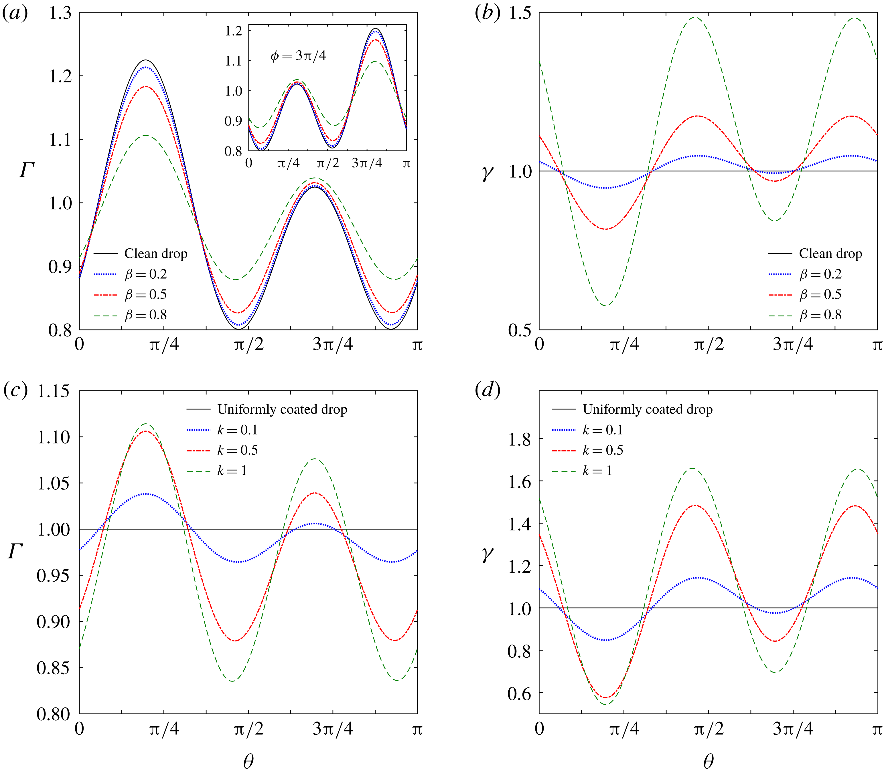
symbolizes an enhancement in the convection of surfactant molecules. Comparing figure 2(a,b), it can be observed that an increase in
 $\unicode[STIX]{x1D6FD}$
causes a sharp increase in surface tension gradients
 $(|\unicode[STIX]{x1D6FE}_{max}-\unicode[STIX]{x1D6FE}_{min}|)$
while the surfactant concentration shows a trend of reaching towards the equilibrium condition,
 $\unicode[STIX]{x1D6E4}=1$
. Similar phenomena were also previously observed by Li & Pozrikidis (Reference Li and Pozrikidis1997) for the case of a surfactant-laden drop in linear shear flow. It is seen that the stronger the surface tension gradient
 $(|\unicode[STIX]{x1D6FE}_{max}-\unicode[STIX]{x1D6FE}_{min}|)$
becomes the more it opposes the convective transport of surfactant molecules. As a result the gradient of surfactant concentration
 $(|\unicode[STIX]{x1D6E4}_{max}-\unicode[STIX]{x1D6E4}_{min}|)$
is reduced and in effect
 $\unicode[STIX]{x1D6E4}$
gets redistributed to a form towards equilibrium.
The limiting condition of
 $k=0$
or
 $Pe=0$
, indicates that surface diffusion of surfactant molecules dominates so that the convection effects become negligible and gradients in surface tension become diminishingly small. This corresponds to a physical situation when the drop surface is uniformly coated with surfactants (Stone & Leal Reference Stone and Leal1990). An increase in the parameter
 $k$
, on the other hand, stands for an increase in the surface Péclet number
 $(Pe)$
for a constant
 $Ca$
(refer to (2.24)). Thus it leads to an increased convective transport of surfactant molecules in a manner such that the opposing effect initiated by an increase in surface tension gradient is surpassed. A coherent observation can be made by studying figure 2(c,d).
Polar distribution of surfactant concentration
 $\unicode[STIX]{x1D6E4}$
defined as
 $(\unicode[STIX]{x1D6E4}=\unicode[STIX]{x1D6E4}^{(0)}+Ca\,\unicode[STIX]{x1D6E4}^{(Ca)}+Ca\,Re_{E}\,\unicode[STIX]{x1D6E4}^{(CaRe_{E})})$
and surface tension (
 $\unicode[STIX]{x1D6FE}$
) for various values of elasticity parameter (
 $\unicode[STIX]{x1D6FD}$
) and the physicochemical constant
 $(k)$
. For all panels
 $\unicode[STIX]{x1D719}=\unicode[STIX]{x03C0}/4$
,
 $(\unicode[STIX]{x1D703}_{e}=\unicode[STIX]{x03C0}/4)$
,
 $Re_{E}=0.2,M=1,Ca=0.2,R=0.1,S=10,x_{d}=4$
,
 $\unicode[STIX]{x1D706}=0.1$
and
 $H=10$
. For (a,b)
 $k=0.5$
while for (c,d)
 $\unicode[STIX]{x1D6FD}=0.8$
is taken.

The electrical parameters have also their parts to play in influencing the surfactant concentration distribution
 $\unicode[STIX]{x1D6E4}(\unicode[STIX]{x1D703},\unicode[STIX]{x1D719})$
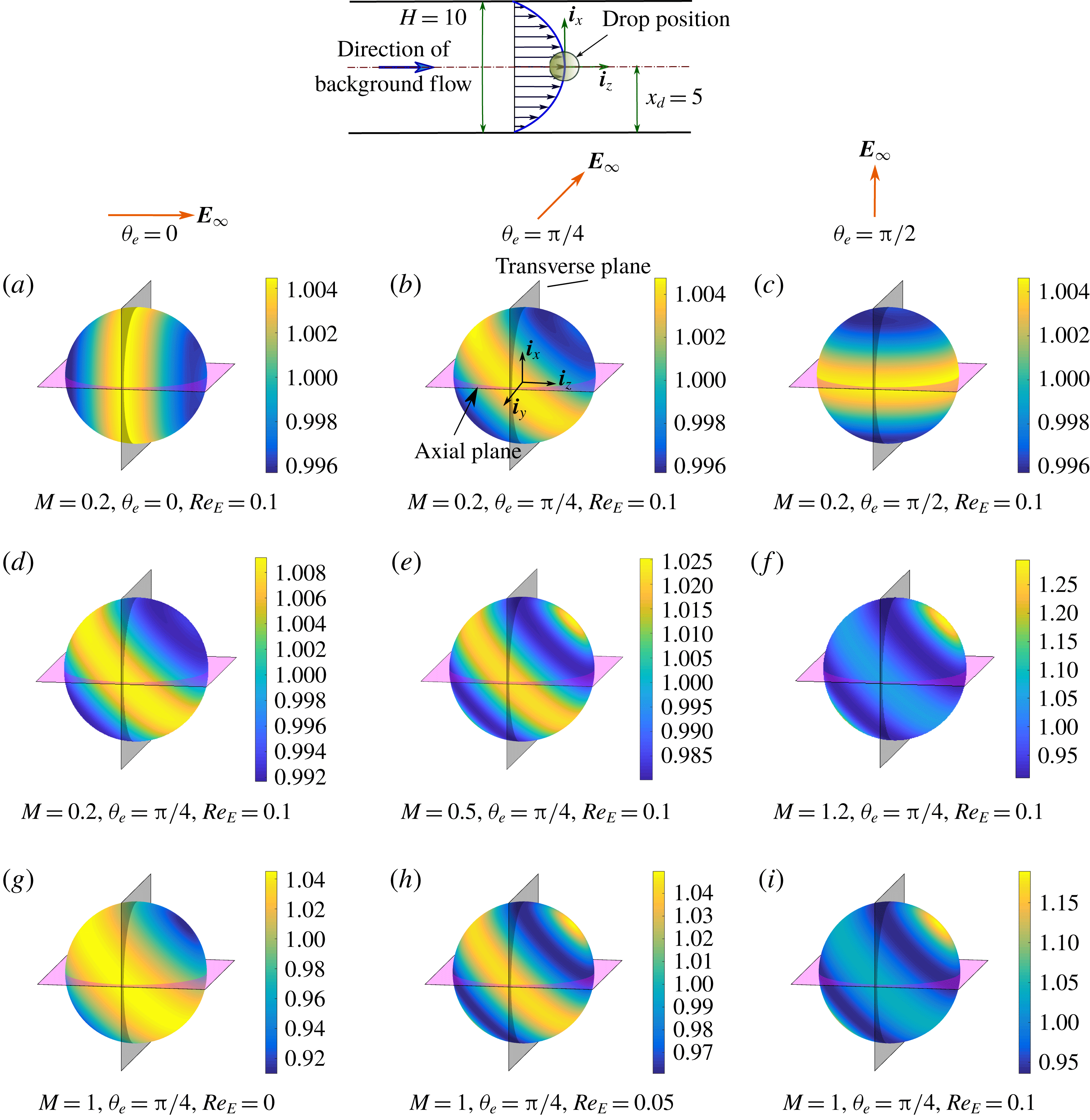
on the drop surface. In figure 3 the effects of both the angle of tilt of the applied electrical field
 $(\unicode[STIX]{x1D703}_{e})$
and the relative importance of the electrical stresses compared to hydrodynamic ones (quantified by Mason number
 $(M)$
), are highlighted. Figure 3(a–c) reveals that the surfactant distribution follows a virtual symmetry axis similar to the applied electric field direction while the maximum and minimum values of the surfactant concentrations on the drop surface remain unaltered. When the Mason number increases not only the values of
 $\unicode[STIX]{x1D6E4}_{max}$
and
 $\unicode[STIX]{x1D6E4}_{min}$
change, but also their locations on the surface are altered. In figure 3(g–i) the effect of intensity of charge convection (quantified by
 $Re_{E}$
) is shown. As the charge convection becomes more and more prominent, similar to the effect due to Mason number, the distribution of surfactant molecules is affected in both qualitative and quantitative manners.
Surfactant concentration (
 $\unicode[STIX]{x1D6E4}=\unicode[STIX]{x1D6E4}^{(0)}+Ca\,\unicode[STIX]{x1D6E4}^{(Ca)}+Ca\,Re_{E}$
 $\unicode[STIX]{x1D6E4}^{(CaRe_{E})}$
) variation on the drop surface for different values of the tilt angle of the applied electric field
 $(\unicode[STIX]{x1D703}_{e})$
, Mason number
 $(M)$
and electrical Reynolds number
 $(Re_{E})$
. In (a–c)
 $\unicode[STIX]{x1D703}_{e}$
is varied; in (d–f)
 $M$
is varied; and in (g–i)
 $Re_{E}$
is varied. Other parameters are
 $Ca=0.2,R=0.1,S=10,\unicode[STIX]{x1D706}=0.1,\unicode[STIX]{x1D6FD}=0.8$
and
 $k=0.5$
. The drop position, applied electric field directions and the axis locations relative to the channel are schematically shown above the panels.

3.1.2 Interfacial charge distribution
We now consider the surfactant-induced alterations in the distribution of accumulated charges on the unreformed drop surface in the presence of a tilted electric field (
 $\unicode[STIX]{x1D703}_{e}=\unicode[STIX]{x03C0}/4$
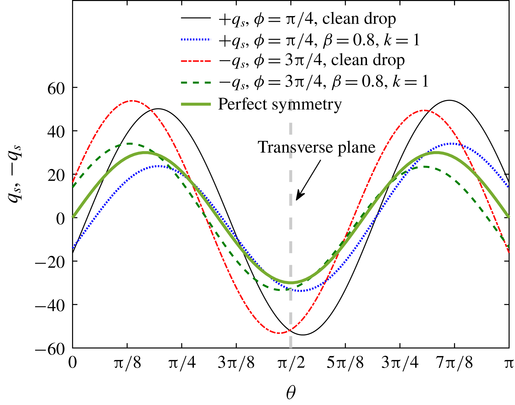
). In figure 4 we plot the polar variation of the surface charge at two symmetrically opposite locations about the axial plane
 $(\unicode[STIX]{x1D719}=\unicode[STIX]{x03C0}/4\text{ and }3\unicode[STIX]{x03C0}/4)$
. Even for the surfactant-free case the surface charge follows an asymmetric distribution about the transverse plane. When the surface is coated with surfactants,
 $q_{S}$
still displays such symmetry-breaking behaviour for both
 $\unicode[STIX]{x1D719}=\unicode[STIX]{x03C0}/4$
and
 $3\unicode[STIX]{x03C0}/4$
, but its distribution pattern is remarkably different. As shown in the preceding section (figure 2
b) an enhancement in surface tension gradients results due to an increase in
 $\unicode[STIX]{x1D6FD}$
. This triggers an enhanced Marangoni flow which further affects the convection of surface charges and a redistribution in the
 $q_{S}(\unicode[STIX]{x1D703})$
results.
Polar distribution of accumulated electrical charge
 $(q_{S}=q_{S}^{(0)}+Re_{E}\,q_{S}^{(Re_{E})})$
for clean as well as surfactant-coated drop in the presence of a tilted electric field
 $(\unicode[STIX]{x1D703}_{e}=\unicode[STIX]{x03C0}/4)$
. Other parameters were taken as
 $Re_{E}=0.2,M=1,R=0.1,S=10,\unicode[STIX]{x1D706}=0.1$
,
 $x_{d}=4$
and
 $H=10$
.

3.1.3 Drop velocity in the cross-stream direction
Even when the charge convection effect is not taken into account, an asymmetry in the surfactant distribution results about the axial plane in the presence of a tilted electric field (shown in figure 3
g). However this asymmetry is not so severe that it alone cannot cause a cross-stream component of the drop velocity and we found
 $U_{d,x}^{(0)}=0$
(refer to the discussion preceding (2.50a
)).
For a clean drop the classical EHD results (Mandal et al.
Reference Mandal, Bandopadhyay and Chakraborty2016c
) revealed that even for a non-deformable drop surface the charge convection effect can create asymmetry in charge distribution about the axial plane. This leads to a transverse component of drop velocity
 $(U_{d,x}^{(Re_{E})}|_{Clean})$
which can either be positive or negative depending on the electrical conductivity and permittivity combinations of the drop-surrounding fluid pair. However in the present case, (2.54) suggests that the factor
 ${\mathcal{F}}_{x}^{(Re_{E})}$
, which quantifies the effect of surfactant on the
 $O(Re_{E})$
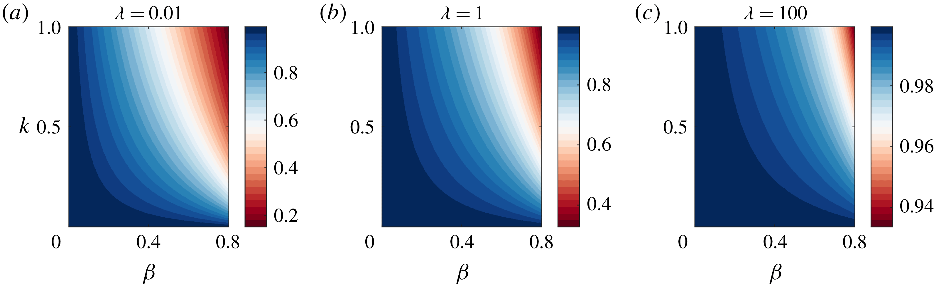
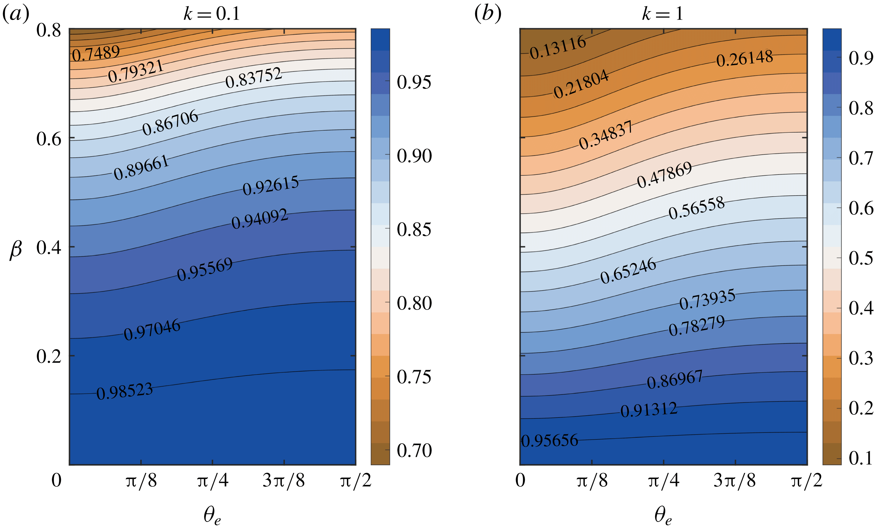
correction to cross-stream velocity, is not influenced by any electrical property of the system. In figure 5(a–c) we have shown the variations of
 ${\mathcal{F}}_{x}^{(Re_{E})}$
with
 $\unicode[STIX]{x1D6FD},k$
and
 $\unicode[STIX]{x1D706}$
.
Variation of the surfactant contribution parameter
 ${\mathcal{F}}_{x}^{(Re_{E})}$
in the
 $\unicode[STIX]{x1D6FD}$
–
 $k$
plane for three different viscosity ratios (
 $\unicode[STIX]{x1D706}$
).

It can be inferred from these figures that magnitude of
 $U_{d,x}^{(Re_{E})}$
always gets reduced by the presence of non-uniform surfactant distribution (i.e.
 ${\mathcal{F}}_{x}^{(Re_{E})}\leqslant 1$
) while the sign of
 $U_{d,x}^{(Re_{E})}$
remains unaltered (i.e.
 ${\mathcal{F}}_{x}^{(Re_{E})}\geqslant 0$
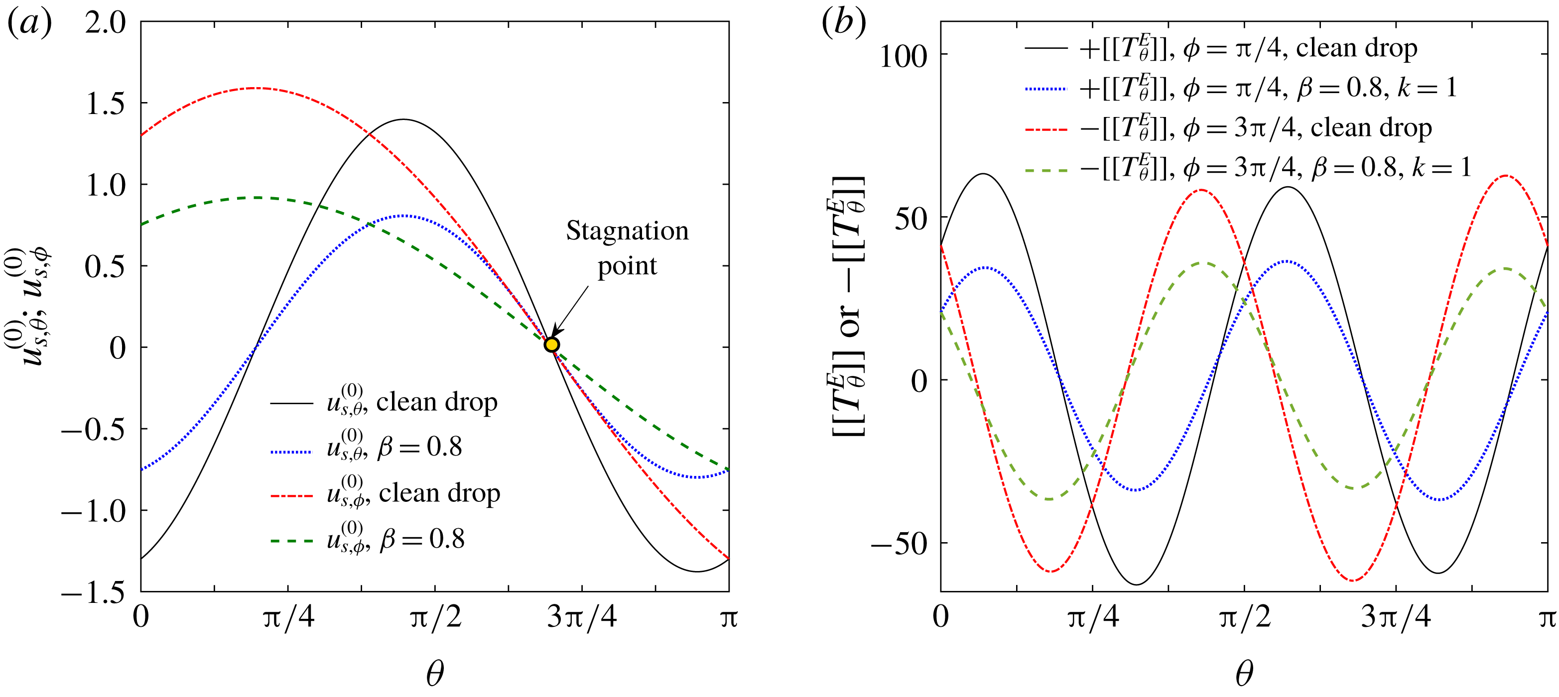
). To analyse the physical mechanism we appeal to figure 4 where it is observed that the surfactant parameters cause remarkable modulations in the asymmetric pattern of the charge distribution about the axial plane. Thus the mechanism of convection of charges due to surface flow is now counteracted by a decrease in the convective flow strength owing to the gradients in the surface tension. As a direct consequence, the electrohydrodynamic flow around the drop is affected severely. This can be visualized by looking into the modulations in leading-order surface velocity
 $u_{S}^{(0)}$
and electrical traction force component
 $([[T_{\unicode[STIX]{x1D703}}^{E}]])$
in figures 13(a) and 13(b), respectively.
Comparing the three cases presented in figure 5(a–c) it is found that surfactant retardation effect is maximum for
 $\unicode[STIX]{x1D706}=0.01$
while the opposite is true for
 $\unicode[STIX]{x1D706}=10$
. When drop fluid shows much less viscosity in comparison to the suspending media, (equivalently the condition
 $\unicode[STIX]{x1D706}\ll 1$
), the drop resembles the behaviour of a bubble and the surfactant contribution factor
 ${\mathcal{F}}_{x}^{(Re_{E})}$
reaches
 $$\begin{eqnarray}\lim _{\unicode[STIX]{x1D706}\rightarrow 0}{\mathcal{F}}_{x}^{(Re_{_{E}})}={\displaystyle \frac{(-756+14(k^{2}+19k-54)\unicode[STIX]{x1D6FD}^{2}+14(-19k+108)\unicode[STIX]{x1D6FD})(-1+\unicode[STIX]{x1D6FD})}{27(2+(k-2)\unicode[STIX]{x1D6FD})^{2}(7+(k-7)\unicode[STIX]{x1D6FD})}}.\end{eqnarray}$$
On the other hand as the drop internal viscosity increases, the internal circulation strength becomes weaker and the Marangoni stress has very little to offer in affecting the circulation behaviour. With
 $\unicode[STIX]{x1D706}\gg 1$
, the drop surface become almost immobile and it behaves as a rigid sphere. In that case the surface convection velocity vanishes. As a consequence both the charge convection and surfactant induced Marangoni effects make diminishingly smaller contributions in controlling the drop migration velocity i.e.
 $\lim _{\unicode[STIX]{x1D706}\rightarrow \infty }U_{d,x}^{(Re_{E})}|_{Clean}=0$
and
 $\lim _{\unicode[STIX]{x1D706}\rightarrow \infty }{\mathcal{F}}_{x}^{(Re_{E})}=1$
. Similar trend of
 ${\mathcal{F}}_{x}^{(Re_{E})}$
is observed in figure 5(c).
3.1.4 Drop velocity in the longitudinal direction
Drop velocity component in the direction parallel to the imposed flow (
 $z$
-direction) for a non-deformable drop can be expressed as
 $U_{d,z}=U_{d,z}^{(0)}+Re_{E}\,U_{d,z}^{(Re_{E})}$
. From mathematical arguments it can be shown that, for the realistic range of the controlling dimensionless parameters
 $(0\leqslant k\leqslant 1,0\leqslant \unicode[STIX]{x1D6FD}\leqslant 0.8,\unicode[STIX]{x1D706}\geqslant 0,c_{2}=-4/H^{2}<0)$
, the term
 ${\mathcal{F}}_{z}^{(0)}$
in (2.50a
) is always a negative quantity. Unlike
 ${\mathcal{F}}_{x}^{(Re_{E})}$
as discussed before,
 ${\mathcal{F}}_{z}^{(Re_{E})}$
is dependent on the direction of the externally applied electric field (please refer to (2.57)). To obtain an overall picture of the surfactant effect, we define a surfactant contribution factor as
 $$\begin{eqnarray}{\mathcal{F}}_{z}^{CC}={\displaystyle \frac{U_{d,z}^{(0)}+Re_{E}\,U_{d,z}^{(Re_{E})}}{U_{d,z}^{(0)}|_{Clean}+Re_{E}\,U_{d,z}^{(Re_{E})}|_{Clean}}},\end{eqnarray}$$
which quantifies the extent to which the longitudinal drop velocity is altered in the presence of surfactant coating.
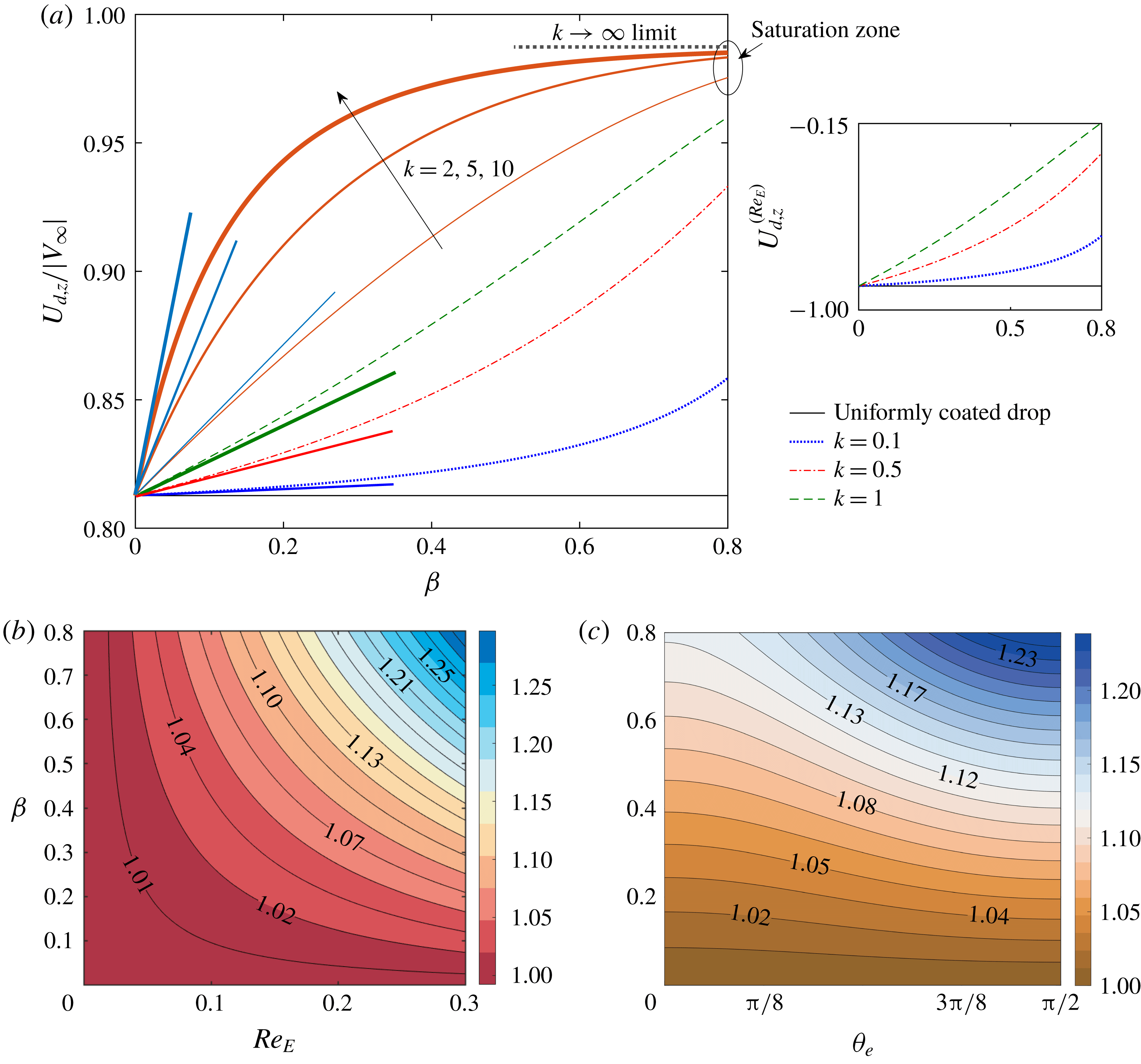
Effect of surfactant parameters on longitudinal drop velocity (defined as
 $U_{d,z}=U_{d,z}^{(0)}+Re_{E}\,U_{d,z}^{(Re_{E})}$
) for a non-deformable drop. (a) Shows the normalized drop velocity versus
 $\unicode[STIX]{x1D6FD}$
for different values of
 $k$
. Here the drop velocity is normalized with respect to the magnitude of the imposed flow velocity at that location
 $|V_{\infty }|$
. The corresponding variation in
 $U_{d,z}^{(Re_{E})}$
is shown at the right of the main panel. In the main panel the nature of the variation of the velocity is shown also for some higher values of the parameter
 $k$
. The straight line segment corresponding to each curve represents the tangent to that line at
 $\unicode[STIX]{x1D6FD}=0$
. The slopes of these lines are physically interpreted as the sensitivity of the drop velocity when the surfactant-induced effects initiate. Here the tilt angle of the applied electric field is taken as
 $\unicode[STIX]{x1D703}_{e}=\unicode[STIX]{x03C0}/4$
. (b) Correction factor
 ${\mathcal{F}}_{z}^{CC}$
variation in the
 $Re_{E}$
–
 $\unicode[STIX]{x1D6FD}$
plane for
 $k=1,\unicode[STIX]{x1D703}_{e}=\unicode[STIX]{x03C0}/4$
. (c) Correction factor
 ${\mathcal{F}}_{z}^{CC}$
variation in the
 $\unicode[STIX]{x1D703}_{e}$
–
 $\unicode[STIX]{x1D6FD}$
plane for
 $k=1.$
Other parameters were taken as
 $\unicode[STIX]{x1D706}=0.1,M=2,Re_{E}=0.2,R=0.1,S=20,x_{d}=4\text{ and }H=10$
.

In figure 6(a) it is observed that the drop lags behind the flow, as observed through the parameter
 $U_{d}/V_{\infty }<1$
. However an increase in the elasticity parameter
 $\unicode[STIX]{x1D6FD}$
or the physicochemical constant
 $k$
causes the axial migration speed to enhance and thereby making the drop to follow the applied flow speed. A non-uniform distribution of surfactant molecules greatly affects the extent of the asymmetry in the charge distribution about the transverse plane (shown in figure 4), thus modifying the asymmetric distribution of tangential electric force itself (see figure 13
b). In turn the drag force on the drop in the longitudinal direction also gets modified, the nature of which is decided by a complex interplay among the electric, hydrodynamic and Marangoni stresses. The sensitivity of the surfactant contribution to the longitudinal velocity is depicted with the slope of the curves at
 $\unicode[STIX]{x1D6FD}=0$
. It is observed that for low values of
 $k(k<1)$
the rate of surfactant-induced enhancement in the
 $U_{d,z}$
shows a fixed trend of rising with the surface elasticity effect. Interestingly, for high values of
 $k$
the enhancement in velocity reaches almost a constant value in the limit of high surface elasticity and becomes insensitive to
 $\unicode[STIX]{x1D6FD}$
. This saturation value of
 $U_{d,z}$
can be obtained by taking the limit
 $\lim _{k\rightarrow \infty }U_{d,z}$
. In this limiting condition, the surface of the drop becomes completely immobilized by the surfactant molecules and the surface velocity tends to zero, rendering the charge convection effect negligible too. Thus in this case the value of the velocity can be approximated as
 $\lim _{k\rightarrow \infty }U_{d,z}=\lim _{k\rightarrow \infty }U_{d,z}^{(0)}=c_{0}+c_{2}/3$
.
Unlike the cross-stream component of velocity, the drop exhibits longitudinal movement for any configuration of the applied electric field
 $0\leqslant \unicode[STIX]{x1D703}_{e}\leqslant \unicode[STIX]{x03C0}/2$
. Following (2.57) it is found that the
 $O(Re_{E})$
axial velocity is dependent on the electric field components, apart from being a function of
 $\unicode[STIX]{x1D6FD},k$
and
 $\unicode[STIX]{x1D706}$
. The parametric dependence of
 ${\mathcal{F}}_{z}^{CC}$
is presented in figure 6
c which shows that the longitudinal drop velocity is enhanced with increasing
 $\unicode[STIX]{x1D6FD}$
for all values of
 $0\leqslant \unicode[STIX]{x1D703}_{e}\leqslant \unicode[STIX]{x03C0}/2$
. Changing the direction of the applied electric field severely affects the surfactant distribution (as shown in figure 3), which in turn modifies the way electrohydrodynamically induced flow interacts with the Marangoni flow. Consequently the resultant interface stress gets altered, thus again modifying the drag force on the drop dictating the drop velocity. Now from figure 5(a) we find that
 $U_{d,z}^{(Re_{E})}$
remains
 ${<}0$
for the current choice of the electrical parameter combination
 $(R=0.1,S=20)$
, but the magnitude of the same
 $(U_{d,z}^{(Re_{E})})$
decreases. Also in figure 15 we find that
 $U_{d,z}^{(Re_{E})}$
gets further reduced if the tilt angle is increased. Although the
 $O(Re_{E})$
longitudinal velocity is associated with the phenomenon of charge convection, the practical effect of the same can only be realized when it is added to the leading-order term to give an overall physical velocity in the
 $z$
direction as
 $U_{d,z}=U_{d,z}^{(0)}+Re_{E}\,U_{d,z}^{(Re_{E})}.$
Now the leading-order velocity
 $U_{d,z}^{(0)}$
is
 ${>}0$
for the said choice of parameters in the figure, with or without surfactant coating. Hence, as a result, the reduction in
 $U_{d,z}$
due to charge convection gets suppressed by Marangoni flow. The effects of
 $Re_{E}$
and
 $\unicode[STIX]{x1D6FD}$
in modifying
 $U_{d,z}$
is provided as a map of the parameter
 ${\mathcal{F}}_{z}^{CC}$
in the
 $Re_{E}-\unicode[STIX]{x1D6FD}$
plane in figure 6(b). It shows that, when the charge convection effect is small, the Marangoni flow shows hardly any influence on
 $U_{d,z}$
. However, as the charge convection effect increases, the Marangoni flow causes more and more augmentation in the longitudinal drop velocity
 $(U_{d,z})$
. Again the increasing behaviour of longitudinal drop velocity with rising surface tension gradient is increasingly prominent as the tilt angle of the applied electric field increases before reaching the maximum in the case of transverse electric field (at
 $\unicode[STIX]{x1D703}_{e}=\unicode[STIX]{x03C0}/2$
) (see figure 6
c).
3.2 Effects on a deformable drop
3.2.1 Drop velocity alteration in the cross-stream direction
Towards explaining the surfactant related effect on the cross-stream velocity of a deformable drop we first look into the possible changes in the electrohydrodynamically induced drop shape deformation that surfactants can bring in. In figure 16(a,b) we have shown the variations in the drop cross-section perpendicular to the lateral migration direction
 $(A_{yz})$
. In the inset of both figures the corresponding drop shapes are also shown. Leaky dielectric drops in another leaky dielectric medium have a tangential component of the electrical force at the drop surface due to induced free charges at the interface. This drives the fluid to flow both interior and exterior to the drop. At the drop-surrounding interface such a flow gives rise to a finite normal viscous stress which acts as a significant contributor to the deforming forces. Now the nature of the electrohydrodynamic force is highly dependent on the parametric combination of
 $R,S$
and
 $\unicode[STIX]{x1D706}$
which was first identified and explained by Taylor (Taylor Reference Taylor1966).
Effect on surfactant parameters on the
 $O(Ca)$
cross-stream velocity
 $(U_{d,x}^{(Ca)})$
. (a)
 $(U_{d,x}^{(Ca)})$
versus
 $\unicode[STIX]{x1D6FD}$
for different values of
 $k$
. In this case
 $R=5,S=0.5$
and
 $\unicode[STIX]{x1D703}_{e}=\unicode[STIX]{x03C0}/4.$
(b) Similar to (a) but with
 $R=0.1,S=10$
. For both (a,b)
 $M=0.1$
was taken. (c) Surfactant contribution parameter
 ${\mathcal{F}}_{x}^{(Ca)}$
with tilt angle
 $\unicode[STIX]{x1D703}_{e}$
for various values of the Mason number
 $(M)$
and
 $R=5,S=0.5$
. The other parameters are
 $\unicode[STIX]{x1D706}=0.1,x_{d}=4$
and
 $H=10$
.

As a consequence the drop assumes two opposite kinds of shape in cases
 $R=5,S=0.5,\unicode[STIX]{x1D706}=0.1$
(figure 16
a) and
 $R=0.1,S=10,\unicode[STIX]{x1D706}=0.1$
(figure 16
b). With respect to the
 $E_{y}$
component of the applied electric field these deformation patterns can classified as oblate and prolate shapes, respectively.
Previously it was observed in figure 2 of § 3.1.1 that the local surface tension
 $(\unicode[STIX]{x1D6FE})$
of the drop reduces at some localized positions where the surfactant concentration becomes high. As a consequence, the drop surface in those locations have to deform more in order maintain a balance of the normal stress (please refer to (2.23)). This mechanism is known as the ‘tip stretching’ phenomenon (Pawar & Stebe Reference Pawar and Stebe1996). Now figure 16(a) shows that for an increase in either of
 $\unicode[STIX]{x1D6FD}$
or
 $k$
, the drop cross-section gets reduced for
 $R=5$
and
 $S=0.5$
and thus
 $U_{d,x}^{(Ca)}$
is expected to increase due to reduced flow resistance. This is in apparent contradiction to the increasing trend of
 $|U_{d,x}^{(Ca)}|$
in figure 7(a). This can be resolved by realizing firstly that the amount of shape change due to surfactants is very low in this case, thus the ‘tip stretching’ plays a very minor role in this case. This is further confirmed from the negligible surface area alteration owing to the presence of surfactants as shown in 17. Secondly, even in the case of a clean drop surface when an electric field is applied it causes a drop deformation and subsequent modifications in charge distribution on the drop surface. This charge distribution gets altered significantly when Marangoni stress comes into play. As a consequence of such phenomena the electrohydrodynamic flow pattern is redistributed in a way that has the potential to affect the drag force on the drop and also the resulting drop velocity magnitude. To exemplify we appeal to figure 13(a) where the significant alterations in the surface flow due to surfactant were captured in terms of changes in the
 $u_{S}^{(0)}$
components. In addition we present figure 14 which shows that the
 $O(Ca)$
correction to the electrohydrodynamic traction force distribution
 $[[\boldsymbol{T}^{E,(Ca)}]]$
also gets modified when the surface elasticity
 $(\unicode[STIX]{x1D6FD})$
varies. In the case of
 $R=5$
and
 $S=0.5$
, the small effect of surfactant-induced deformation is surpassed by the above effect.
Contrary to the above, for a choice of parameters
 $R=0.1,S=10$
, the drop cross-section increases with surfactant effects (refer to figure 16
b) although again the amount of modulation is very low. This in turn competes with the electrohydrodynamic flow modification effect and finally a reduction in
 $|U_{d,x}^{(Ca)}|$
is observed in figure 7(b).
Figure 7(c) depicts an increasing trend of surfactant effect with an increase in the Mason number. This can be explained as follows. As the Mason number increases charge convection becomes more and more prominent and causes tremendous changes in the surfactant distribution. This leads to a greater gradient in surface tension and the Marangoni stress has a greater scope to influence the drop velocity. It (figure 7
c) also suggests, when the applied electric field is either axial
 $(\unicode[STIX]{x1D703}_{e}=0)$
or transverse
 $(\unicode[STIX]{x1D703}_{e}=\unicode[STIX]{x03C0}/2)$
, that changing the Mason number
 $(M)$
has no effect on the surfactant contribution. This is due to the fact that in those cases the deformation-triggered cross-stream velocity is not at all affected by electrical effects and is generated solely due to hydrodynamic effects (Mandal et al.
Reference Mandal, Bandopadhyay and Chakraborty2016c
). When the electric field is applied at an angle
 $\unicode[STIX]{x1D703}_{e}>0$
, the parameter
 ${\mathcal{F}}_{x}^{(Ca)}$
decreases continuously before reaching at a minimum at
 $\unicode[STIX]{x1D703}_{e}=\unicode[STIX]{x03C0}/4$
. In a symmetric manner, a further increase in tilt angle causes
 ${\mathcal{F}}_{x}^{(Ca)}$
to increases, physically manifesting as a fall in the surfactant-induced retardation effect.
3.2.2 Drop velocity alteration in the longitudinal direction
It is evident from figure 8(a) that in the absence of surfactant-induced Marangoni effects, the drop lags behind the flow (i.e.
 $U_{d,z}/|V_{\infty }|<1$
) for the choice of electrohydrodynamic parameters. An increase in either
 $\unicode[STIX]{x1D6FD}$
or
 $k$
indicates a corresponding enhancement in the Marangoni stresses. Now the variation of projected area perpendicular to the drop motion direction shows that
 $A_{xy}$
increases with increasing values of surfactant parameters (shown in figure 18). Similar to the discussion in the preceding section (3.1.3), a combination of the mechanisms of tip stretching and redistribution of electrohydrodynamic stresses on the deformed surface causes an increase in the drag force on the drop in a direction opposite to its longitudinal motion. This creates further retardation in the longitudinal motion of the drop.
Similar to the case of
 $O(Re_{E})$
(§ 3.1.4), in order to quantify the surfactant-induced modifications in the longitudinal drop velocity where the shape deformation is the dominant mechanism, we define another overall surfactant contribution parameter as
 $$\begin{eqnarray}{\mathcal{F}}_{z}^{D}={\displaystyle \frac{U_{d,z}^{(0)}+Ca\,U_{d,z}^{(Ca)}}{U_{d,z}^{(0)}|_{Clean}+Ca\,U_{d,z}^{(Ca)}|_{Clean}}},\end{eqnarray}$$
and investigate the effects of the electrical property ratios
 $R$
and
 $S$
in figure 8(b). It is observed that for the choice of parameters in figure 8(a)
 $(R=0.1,S=20)$
, a significant effect of the surfactant results. However, for some other choices similar to those used in the case of
 $O(Ca)$
cross-stream velocity (
 $(R,S)=(5,0.5)$
and
 $(R,S)=(0.1,10)$
) in § 3.2.1, the surfactants play a very minimal role in altering the longitudinal drop velocity (
 $U_{d,z}=U_{d,z}^{(0)}+Ca\,U_{d,z}^{(Ca)}$
). This indicates that the capability of surface-active agents to modify the drop motion in each direction can be selectively tuned with a suitable choice of electrical conductivity and permittivity ratios of the drop-surrounding fluid pair.
(a) Variation of longitudinal drop velocity defined as
 $U_{d,z}=U_{d,z}^{(0)}+Ca\,U_{d,z}^{(Ca)}$
, with
 $\unicode[STIX]{x1D6FD}$
for various
 $k$
. Again the drop velocity is normalized with respect to the magnitude of the imposed flow velocity at that location
 $|V_{\infty }|$
. Here
 $R=0.1$
and
 $S=20$
. (b) Variation of the surfactant contribution factor
 ${\mathcal{F}}_{z}^{D}$
in the
 $R$
–
 $S$
plane. The red, yellow and green circles represent the three cases
 $R=0.1,S=20;R=0.1,S=10$
and
 $R=5,S=0.5$
, respectively. The other parameters were chosen as
 $\unicode[STIX]{x1D706}=0.1,M=1,Ca=0.2,x_{d}=4,H=10$
and
 $\unicode[STIX]{x1D703}_{e}=\unicode[STIX]{x03C0}/4$
.

3.3 The high Péclet limit
The
 $O(Re_{E})$
surfactant contribution terms in both the components of velocity at
 $O(Re_{E})$
(as shown in (2.54) and (2.57)) vanish in the high
 $Pe$
limit. In this limit, the surface of the drop becomes completely immobilized by the diffusing surfactant molecules and the surface velocity tends to zero, rendering the charge convection effect negligible too. Thus, in the advection dominated regime of the surfactant transport, the cross-stream component of the velocity is solely generated from the deformation of the drop, since the charge convection effect does not contribute to the symmetry-breaking mechanism in this case. In the high
 $Pe$
limit, the expression of
 $O(Ca)$
cross-stream velocity becomes simplified and is given as
 $$\begin{eqnarray}\displaystyle U_{d,x}^{(Ca)} & = & \displaystyle {\textstyle \frac{1}{4}}c_{2}\left({\textstyle \frac{2}{9}}\left(\unicode[STIX]{x1D706}+14\right)\left(R+2\right)^{2}c_{1}+\left(R^{2}+6R-8S+1\right)E_{x}E_{z}M\right)\nonumber\\ \displaystyle & & \displaystyle +\,{\displaystyle \frac{c_{2}\left({\textstyle \frac{2}{9}}\left(-3\unicode[STIX]{x1D706}-17\right)\left(R+2\right)^{2}c_{1}+\left(-4R+4S\right)E_{x}E_{z}M\right)}{4\unicode[STIX]{x1D6FD}\,\left(R+2\right)^{2}\left(\unicode[STIX]{x1D706}+4\right)}}.\end{eqnarray}$$
From figure 9, it can be observed that for different choices of the electrical property ratios, the value of the
 $O(Ca)$
cross-stream velocity
 $U_{d,x}^{(Ca)}$
decreases with an increase in the surfactant parameter
 $\unicode[STIX]{x1D6FD}$
and finally saturates towards a vanishing limit. This can be explained from (3.4) where the
 $U_{d,x}^{(Ca)}$
is found to be inversely proportional to
 $\unicode[STIX]{x1D6FD}$
. Comparing this with figure 7(a,b), it is observed that, in the high
 $Pe$
limit, the magnitude of the cross-stream velocity becomes significantly higher than the low
 $Pe$
case.
Variation in the
 $O(Ca)$
cross-stream migration velocity with the surface elasticity parameter
 $\unicode[STIX]{x1D6FD}$
for different combinations of the electrical property ratios (
 $R,S$
). Here the other parameters are taken as
 $\unicode[STIX]{x1D706}=0.1,M=0.1,x_{d}=4,H=10$
and
 $\unicode[STIX]{x1D703}_{e}=\unicode[STIX]{x03C0}/4.$

3.4 Drop trajectory
Effect of surfactant on the drop trajectory when both the charge convection and shape deformation are considered. (a,b) Drop trajectory for various elasticity parameters
 $(\unicode[STIX]{x1D6FD})$
and
 $k=1$
. (c,d) Variation of final steady state transverse position of the drop
 $x_{d,\infty }$
in the
 $\unicode[STIX]{x1D6FD}$
–
 $k$
plane. For (a,c)
 $R=5$
,
 $S=0.5$
,
 $M=0.5$
and for (b,d)
 $R=0.5,S=5,M=0.1$
. The other parameters are given as
 $\unicode[STIX]{x1D706}=0.1,\unicode[STIX]{x1D703}_{e}=\unicode[STIX]{x03C0}/4,Ca=0.1$
and
 $Re_{E}=0.1$
.

Variation in the final steady-state transverse position of the drop with respect to the surfactant-free case
 $(x_{d,\infty }/x_{d,\infty ,Clean})$
for varying direction of the applied electric field and various values of Mason number
 $(M)$
. For (a)
 $R=5,S=0.5$
and for (b)
 $R=0.5,S=5$
. The other parameters are
 $\unicode[STIX]{x1D706}=0.1,\unicode[STIX]{x1D6FD}=0.8,k=1;Re_{E}=0.1\text{ and }$
 $Ca=0.1$
.

The surfactant distribution, surface charge and the interfacial flow velocity are altered in such a way that the drop begins to move in the longitudinal as well as in the cross-stream direction. Under the quasi-steady-state assumption the drop trajectory was obtained in § 2.3.2. Figure 10(a) shows that an increase in
 $\unicode[STIX]{x1D6FD}$
causes the drop to settle down to a steady-state transverse location much lower than a clean drop. This can be explained again by following figure 19(a), which shows that the magnitude of the cross-stream migration velocity
 $(|U_{d,x}|)$
is reduced for an increase in the elasticity parameter
 $(\unicode[STIX]{x1D6FD})$
. In addition, the time required to reach the final steady-state position
 $t_{S}$
is increased for the same conditions. With another parameter choice (
 $R=0.5,S=5,M=0.1$
), figure 10(b) demonstrates that the downward drop motion away from the centreline is slowed down and finally it reaches a lateral position
 $(x_{d,\infty })$
which is much higher than a clean drop. Variation of final steady-state transverse position of the drop
 $x_{d,\infty }$
in the
 $\unicode[STIX]{x1D6FD}$
–
 $k$
plane is demonstrated in figure 10(c,d). It is observable from these figures that the final drop position is almost insensitive to surface elasticity (
 $\unicode[STIX]{x1D6FD}$
) for low values of
 $k$
. However, the effect of
 $\unicode[STIX]{x1D6FD}$
on
 $x_{d,\infty }$
is of importance when the parameter
 $k$
also takes a high value.
Comparing figure 11(a,b), it is found that for achieving a similar change in
 $x_{d,\infty }$
with different values of
 $R,S$
, the required range of Mason number is significantly different. This suggests that the surfactant-induced change in steady-state drop position in the lateral direction is dictated by a complex interplay among electrical properties. As the electrical effects increase compared to the hydrodynamic effect, presence of the surfactant molecules can alter the final drop location in a more dominant fashion.
The combined action of charge convection and the shape deformation leads to a resultant cross-stream velocity defined as
 $U_{d,x}=Re_{E}\,U_{d,x}^{(Re_{E})}+Ca\,U_{d,x}^{(Ca)}$
. For a choice of
 $R=5,S=0.5,M=0.5$
,
 $U_{d,x}$
is
 ${>}0$
(shown in figure 19
a) and hence the drop trajectory shows a behaviour where the drop migrates downwards away from the centreline. For the other choice of parameters, as shown in figure 19(b), the sign of
 $U_{d,x}$
is just the reverse
 $(U_{d,x}<0)$
. Accordingly, the drop motion shows an upward trend in figure 10(b).
To highlight the most important results of the present study, we finally represent the general case when both charge convection and shape deformation effects are present in the system. The combined consequences of various mechanisms for the drop velocity are presented in figure 12. It shows that, based on the variations of the surfactant-induced enhancement or attenuation of the drop velocity as well as its sensitivity with the Marangoni effect, different operating regimes can be distinguished for the
 $(Re_{E},Ca)$
values.
4 Experimental perspective
The present theoretical model has been built up on the assumption of a parametric space where the different dimensionless numbers lie in the range
 $Ca\ll 1,Re_{E}\ll 1,Pe\ll 1$
and
 $M\sim O(1)$
. To connect to a practical experimental set-up we consider a silicon oil drop of diameter,
 $2a=50~\unicode[STIX]{x03BC}\text{m}$
migrating through a channel of height
 $\widetilde{H}=500~\unicode[STIX]{x03BC}\text{m}$
and the channel centreline velocity is
 $\widetilde{V}_{0}=10^{-4}~\text{m}~\text{s}^{-1}$
, which are commonly found in microfluidic experiments (e.g. Link et al. (Reference Link, Grasland-Mongrain, Duri, Sarrazin, Cheng, Cristobal, Marquez and Weitz2006)). A typical experimental set-up can be designed where monodispersed drops are produced with the help of a T-shaped device (Baroud et al.
Reference Baroud, Gallaire and Dangla2010) and drop size can be effectively controlled by controlling the flow rates of the two streams in the co-flowing configuration. The electric field may be incorporated by creating patterns on the indium tin oxide (ITO) electrodes adjacent to the microchannel (Link et al.
Reference Link, Grasland-Mongrain, Duri, Sarrazin, Cheng, Cristobal, Marquez and Weitz2006) through which the drops are migrating. Let us consider the continuous medium to be castor oil mixed with 2 wt % ethyl alcohol (Ha & Yang Reference Ha and Yang2000) and the drop surface is covered with a non-ionic bulk insoluble surfactant such as Triton X-100 (Santra et al.
Reference Santra, Das, Das and Chakraborty2018) or Tween 60 (Ha & Yang Reference Ha and Yang1998). We choose the following property values as per the experiments of Ha & Yang (Reference Ha and Yang2000):
 $\unicode[STIX]{x1D70E}_{e}=6.6\times 10^{-10}~\text{S}~\text{m}^{-1},\unicode[STIX]{x1D716}_{e}=5.2\unicode[STIX]{x1D716}_{0}$
(where
 $\unicode[STIX]{x1D716}_{0}$
is the free space permittivity),
 $\unicode[STIX]{x1D707}_{e}=0.85\,\text{Pa s}$
and clean drop surface tension
 $\widetilde{\unicode[STIX]{x1D6FE}}_{c}=4.6~\text{mN}~\text{m}^{-1}$
. Now, the equilibrium surface tension of a contaminated drop is related to
 $\widetilde{\unicode[STIX]{x1D6FE}}_{c}$
by the relation
 $\widetilde{\unicode[STIX]{x1D6FE}}_{eq}=\widetilde{\unicode[STIX]{x1D6FE}}_{c}(1-\unicode[STIX]{x1D6FD})$
. Within the practical range of
 $0\leqslant \unicode[STIX]{x1D6FD}\leqslant 0.8$
(Stone & Leal Reference Stone and Leal1990) we choose
 $\unicode[STIX]{x1D6FD}=0.8$
. It is to be noted here that the diffusivity value we are concerned with is the surface diffusivity
 $(D_{S})$
of the surfactant molecules (Leal Reference Leal2007) which is different from the bulk diffusivity
 $(D_{b})$
. The surface diffusivity values of surfactants have been reported in the literature (Valkovska & Danov Reference Valkovska and Danov2000) in the range of
 $D_{S}\sim 10^{-9}$
to
 $10^{-8}~\text{m}^{2}~\text{s}^{-1}$
which are roughly one order of magnitude higher than the bulk diffusivity. Considering the characteristic value of the DC electric field as
 $\widetilde{E}_{0}=2~\text{kV}~\text{cm}^{-1}$
(Xu & Homsy Reference Xu and Homsy2006), density of the external fluid
 $(\unicode[STIX]{x1D70C}_{e})\sim 950~\text{kg}~\text{m}^{-3}$
and
 $D_{S}=10^{-8}~\text{m}^{2}~\text{s}^{-1}$
we obtain
 $Re=\unicode[STIX]{x1D70C}_{e}\widetilde{V}_{0}a/\unicode[STIX]{x1D707}_{e}=2\times 10^{-6},M=0.54,Ca=0.09,Re_{E}=0.28$
and
 $Pe=0.25$
. Hence the experimental fluid pairs mentioned above may yield the appropriate values of the dimensionless quantities used in the present study.
Surfactant-induced modifications in cross-stream (a) and longitudinal (b) drop velocity components when both charge convection and shape deformation are considered. Other parameters are
 $\unicode[STIX]{x1D706}=0.1,\unicode[STIX]{x1D6FD}=0.8,k=1,\unicode[STIX]{x1D703}_{e}=\unicode[STIX]{x03C0}/4$
,
 $M=2,R=0.1\text{ and }S=10$
. Different surfactant-sensitive regimes for velocity variation are shown in the panels.

Recent experiments (Zhang et al. Reference Zhang, He, Ghadiri and Hassanpour2015; Ervik et al. Reference Ervik, Penne, Hellesø, Munkejord and Müller2018) investigating surfactant effects on electrohydrodynamics have investigated the various aspects of drop dynamics. However these studies considered aqueous drops in an oil medium. Recently Santra et al. (Reference Santra, Das, Das and Chakraborty2018) investigated the drop migration in a channel flow modulated by the surfactant-induced Marangoni effects for similar fluid pairs. Such a system is characterized as a perfectly conducting drop in a leaky dielectric fluid and has no tangential component of electric field at the drop surface. Hence a charge convection effect is absent in these cases. In stark contrast, the oil-in-oil systems characterized by leaky dielectric drops in another leaky dielectric medium have a tangential component of the electrical force at the drop surface due to induced free charges at the interface. This drives the fluid to flow both interior and exterior to the drop. The surfactant effects on deformation and burst of liquid drops in such a system were experimentally demonstrated only by Ha & Yang (Reference Ha and Yang1995). This indicates that enough scope exists in the experimental investigation of surfactant effects on the migration characteristics of electrically actuated leaky dielectric drops in another leaky dielectric medium flowing through a channel. In this context the present analysis may turn out to be of immense interest in selecting and optimizing various physical variables pertinent to a detailed experimental study.
5 Conclusions
We have considered a practically relevant situation of electrically modulated droplet motion in Poiseuille flow, under the influence of non-ionic surfactants. The hydrodynamic equations in the creeping flow limit are solved concurrently with the electrical potential and the convection–diffusion equation of surfactant transport. The obtained solution of the velocity and pressure fields inside both the drop and the carrier fluid are then utilized to solve the normal stress balance equation. Thereafter, a description of the deformed shape is obtained within the purview of the small deformation theory. Finally, a description of the drop trajectory
 $(x_{d}(t),z_{d}(t))$
is provided in the ‘quasi-steady-state’ condition. Consequently, the effect of various electrical
 $(R,S,M,\unicode[STIX]{x1D703}_{e},Re_{E})$
and surfactant related parameters
 $(\unicode[STIX]{x1D6FD},k,\unicode[STIX]{x1D706})$
are demonstrated and possible physical mechanisms are critically investigated. The important observations can be summarized as follows:
(i) The surfactant distribution is found to be significantly affected by the electrical parameters such as
$Re_{E},M$
and
$\unicode[STIX]{x1D703}_{e}$
. Due to a complex coupled nature of the surfactant transport and charge convection mechanisms, the surface tension gradients get enhanced with an augmentation in the charge convection. Similarly, with increasing dominance of the electrical stresses relative to the hydrodynamic stresses (quantified by
$M$
), the surface tension variation
$(|\unicode[STIX]{x1D6FE}_{max}-\unicode[STIX]{x1D6FE}_{min}|)$
gets increased. Also, the nature of surfactant distribution closely follows the direction of the applied electric field
$(\unicode[STIX]{x1D703}_{e})$
.(ii) Owing to a noticeable influence of the surfactant distribution on the electrohydrodynamic flow pattern, the accumulation of surface charges is remarkably changed. With an increased sensitivity of the surface tension on the surfactant concentration (increasing
$\unicode[STIX]{x1D6FD}$
), the drop surface gets depleted of charges in some places, while more accumulation is caused in some other locations.(iii) The magnitude of the cross-stream drop velocity due to asymmetric charge distribution at finite
$Re_{E},$
$(U_{d,x}^{(Re_{E})})$
, always reduces due to the Marangoni effect. Notably the surfactant-induced modification is not affected by the electrical parameters. When the drop internal viscosity is too high as compared to the surrounding fluid
$(\unicode[STIX]{x1D706}\ll 1)$
, the Marangoni effect is much stronger while it diminishes as
$\unicode[STIX]{x1D706}\rightarrow \infty$
.(iv) The surfactant effect on the shape deformation triggers a cross-stream migration velocity
$(U_{d,x}^{(Ca)})$
, which is of maximum intensity when the tilt angle
$\unicode[STIX]{x1D703}_{e}$
of the applied electric field is
$\unicode[STIX]{x03C0}/4$
. The said effect has negligible influence as the external electric field approaches either a perfect axial
$(\unicode[STIX]{x1D703}_{e}=0)$
or lateral direction
$(\unicode[STIX]{x1D703}_{e}=\unicode[STIX]{x03C0}/2)$
. A further enhancement in such effect results with increasing value of the Mason number
$(M)$
.(v) The quasi-steady-state drop trajectory, under the simultaneous action of a background plane Poiseuille flow and a tilted electric field, is also greatly influenced by the non-uniform distribution of surface-active molecules along the surface. The surfactant effects, quantified by an increase in
$\unicode[STIX]{x1D6FD}$
or
$k$
, can either cause the drop to move towards or away from the channel centreline depending on the particular choice of parameters
$R$
and
$S$
. Similar to some other important quantities, the surfactant-induced relative increase or decrease in the steady-state final transverse position of the drop is increasingly pronounced at higher values of the Mason number
$(M)$
and near
$\unicode[STIX]{x1D703}_{e}=\unicode[STIX]{x03C0}/4$
. The time required for the final steady-state transverse position in the channel
$(t_{S})$
is reduced in the presence of the surfactant-induced Marangoni stress.


To summarize, our study reveals that adding non-ionic surfactant to the surface of an electric field actuated drop in a plane Poiseuille flow provides a means for selectively controlling the velocity components. In effect, the electrical property ratios
 $(R,S)$
, the Mason number
 $(M)$
and the tilt angle
 $(\unicode[STIX]{x1D703}_{e})$
of the externally applied uniform electric field bring about remarkable changes in the surfactant effects. In practice, such physical consequences can be exploited in achieving an additional degree of control in optimizing drop motion through confined microfluidic passages.
Supplementary material
Supplementary material is available at https://doi.org/10.1017/jfm.2019.236.
Appendix A. Harmonic constants
$(\unicode[STIX]{x1D6E4}_{n,m}^{(Ca)})$
in (2.49)

 $$\begin{eqnarray}\left.\begin{array}{@{}c@{}}\unicode[STIX]{x1D6E4}_{1,0}^{(Ca)}=-{\displaystyle \frac{k\,\left(-1+\unicode[STIX]{x1D6FD}\right)c_{2}}{k\,\unicode[STIX]{x1D6FD}-3\,\unicode[STIX]{x1D6FD}\,\unicode[STIX]{x1D706}-2\,\unicode[STIX]{x1D6FD}+3\,\unicode[STIX]{x1D706}+2}};\qquad \unicode[STIX]{x1D6E4}_{1,1}^{(Ca)}=0;\\ \unicode[STIX]{x1D6E4}_{2,0}^{(Ca)}={\displaystyle \frac{3M\left(E_{x}^{2}-2\,{E_{z}}^{2}\right)\left(-1+\unicode[STIX]{x1D6FD}\right)\left(R-S\right)k}{2\left(\left(k-5\,\unicode[STIX]{x1D706}-5\right)\unicode[STIX]{x1D6FD}+5\,\unicode[STIX]{x1D706}+5\right)\left(R+2\right)^{2}}};\\ \unicode[STIX]{x1D6E4}_{2,1}^{(Ca)}=-{\displaystyle \frac{\left(-1+\unicode[STIX]{x1D6FD}\right)\left(18\,RME_{x}E_{z}-18\,MSE_{x}E_{z}+5\,R^{2}c_{1}+20\,Rc_{1}+20\,c_{1}\right)k}{6\left(k\,\unicode[STIX]{x1D6FD}-5\,\unicode[STIX]{x1D6FD}\,\unicode[STIX]{x1D706}-5\,\unicode[STIX]{x1D6FD}+5\,\unicode[STIX]{x1D706}+5\right)\left(R+2\right)^{2}}};\\ \unicode[STIX]{x1D6E4}_{2,2}^{(Ca)}=-{\displaystyle \frac{3M{E_{x}}^{2}\left(-1+\unicode[STIX]{x1D6FD}\right)\left(R-S\right)k}{4\left(\left(k-5\,\unicode[STIX]{x1D706}-5\right)\unicode[STIX]{x1D6FD}+5\,\unicode[STIX]{x1D706}+5\right)\left(R+2\right)^{2}}};\\ \unicode[STIX]{x1D6E4}_{3,0}^{(Ca)}={\displaystyle \frac{7k\,\left(-1+\unicode[STIX]{x1D6FD}\right)c_{2}}{\left(12\,k-84\,\unicode[STIX]{x1D706}-84\right)\unicode[STIX]{x1D6FD}+84\,\unicode[STIX]{x1D706}+84}};\qquad \unicode[STIX]{x1D6E4}_{3,1}^{(Ca)}=0;\\ \unicode[STIX]{x1D6E4}_{3,2}^{(Ca)}=-{\displaystyle \frac{7k\,\left(-1+\unicode[STIX]{x1D6FD}\right)c_{2}}{\left(72\,k-504\,\unicode[STIX]{x1D706}-504\right)\unicode[STIX]{x1D6FD}+504\,\unicode[STIX]{x1D706}+504}}\quad \text{and}\quad \unicode[STIX]{x1D6E4}_{3,3}^{(Ca)}=0.\end{array}\right\}\end{eqnarray}$$
In the high
 $Pe$
limit the above expressions transform to
 $$\begin{eqnarray}\left.\begin{array}{@{}c@{}}\unicode[STIX]{x1D6E4}_{1,0}^{(Ca)}={\displaystyle \frac{\left(1-\unicode[STIX]{x1D6FD}\right)c_{2}}{\unicode[STIX]{x1D6FD}}};\qquad \unicode[STIX]{x1D6E4}_{1,1}^{(Ca)}=0;\\ \unicode[STIX]{x1D6E4}_{2,0}^{(Ca)}={\displaystyle \frac{3M\left({E_{x}}^{2}-2\,{E_{z}}^{2}\right)\left(-1+\unicode[STIX]{x1D6FD}\right)\left(R-S\right)}{2\unicode[STIX]{x1D6FD}\left(R+2\right)^{2}}};\\ \unicode[STIX]{x1D6E4}_{2,1}^{(Ca)}=-{\displaystyle \frac{\left(-1+\unicode[STIX]{x1D6FD}\right)\left(18\,RME_{x}E_{z}-18\,MSE_{x}E_{z}+5\,R^{2}c_{1}+20\,Rc_{1}+20\,c_{1}\right)}{6\unicode[STIX]{x1D6FD}\left(R+2\right)^{2}}};\\ \unicode[STIX]{x1D6E4}_{2,2}^{(Ca)}=-{\displaystyle \frac{3M{E_{x}}^{2}\left(-1+\unicode[STIX]{x1D6FD}\right)\left(R-S\right)}{4\unicode[STIX]{x1D6FD}\left(R+2\right)^{2}}};\\ \unicode[STIX]{x1D6E4}_{3,0}^{(Ca)}={\displaystyle \frac{7\,\left(-1+\unicode[STIX]{x1D6FD}\right)c_{2}}{12\unicode[STIX]{x1D6FD}}};\qquad \unicode[STIX]{x1D6E4}_{3,1}^{(Ca)}=0;\\ \unicode[STIX]{x1D6E4}_{3,2}^{(Ca)}=-{\displaystyle \frac{7\,\left(-1+\unicode[STIX]{x1D6FD}\right)c_{2}}{72\unicode[STIX]{x1D6FD}}}\quad \text{and}\quad \unicode[STIX]{x1D6E4}_{3,3}^{(Ca)}=0.\end{array}\right\}\end{eqnarray}$$
Appendix B. Harmonic constants
$(L_{n,m}^{(Ca)})$
in (2.51)

 $$\begin{eqnarray}\left.\begin{array}{@{}c@{}}L_{2,0}^{(Ca)}=L_{2,0}^{(Ca)}|_{Clean}+{\displaystyle \frac{3\,M\left({2E_{z}}^{2}-\,{E_{x}}^{2}\right)k\,\unicode[STIX]{x1D6FD}\,\left(\unicode[STIX]{x1D706}+4\right)\left(R-S\right)}{40\left(\,\unicode[STIX]{x1D706}+1\right)\left(\left(-5\,\unicode[STIX]{x1D6FD}+5\right)\unicode[STIX]{x1D706}+5+\left(k-5\right)\unicode[STIX]{x1D6FD}\right)\left(R+2\right)^{2}}};\\ L_{2,1}^{(Ca)}=L_{2,1}^{(Ca)}|_{Clean}+{\displaystyle \frac{3\,k\,\unicode[STIX]{x1D6FD}\,\left(\unicode[STIX]{x1D706}+4\right)\left({\displaystyle \frac{5\,\left(R+2\right)^{2}c_{1}}{18}}+ME_{x}E_{z}\left(R-S\right)\right)}{\left(20\,\unicode[STIX]{x1D706}+20\right)\left(\left(-5\,\unicode[STIX]{x1D6FD}+5\right)\unicode[STIX]{x1D706}+5+\left(k-5\right)\unicode[STIX]{x1D6FD}\right)\left(R+2\right)^{2}}};\\ L_{2,2}^{(Ca)}=L_{2,2}^{(Ca)}|_{Clean}+{\displaystyle \frac{3\,M{E_{x}}^{2}k\,\unicode[STIX]{x1D6FD}\,\left(\unicode[STIX]{x1D706}+4\right)\left(R-S\right)}{80\,\left(R+2\right)^{2}\left(\unicode[STIX]{x1D706}+1\right)\left(\left(-5\,\unicode[STIX]{x1D6FD}+5\right)\unicode[STIX]{x1D706}+5+\left(k-5\right)\unicode[STIX]{x1D6FD}\right)}};\\ L_{3,0}^{(Ca)}=L_{3,0}^{(Ca)}|_{Clean}-{\displaystyle \frac{k\,\unicode[STIX]{x1D6FD}\,c_{2}\left(2\,\unicode[STIX]{x1D706}+5\right)}{\left(120\,\unicode[STIX]{x1D706}+120\right)\left(\left(-7\,\unicode[STIX]{x1D6FD}+7\right)\unicode[STIX]{x1D706}+7+\left(k-7\right)\unicode[STIX]{x1D6FD}\right)}};\\ \text{and}\quad L_{3,2}^{(Ca)}=L_{3,2}^{(Ca)}|_{Clean}+{\displaystyle \frac{k\,\unicode[STIX]{x1D6FD}\,c_{2}\left(2\,\unicode[STIX]{x1D706}+5\right)}{\left(720\,\unicode[STIX]{x1D706}+720\right)\left(\left(-7\,\unicode[STIX]{x1D6FD}+7\right)\unicode[STIX]{x1D706}+7+\left(k-7\right)\unicode[STIX]{x1D6FD}\right)}},\end{array}\right\}\end{eqnarray}$$
where in each case the first term describes the same harmonic for a surfactant-free drop
 $(\unicode[STIX]{x1D6FD}=0)$
and the second term stands for the contribution due to surfactant.
In the high
 $Pe$
limit the above expressions transform to
 $$\begin{eqnarray}\left.\begin{array}{@{}c@{}}L_{2,0}^{(Ca)}=L_{2,0}^{(Ca)}|_{Clean}+{\displaystyle \frac{3\,M\left({2E_{z}}^{2}-\,{E_{x}}^{2}\right)\,\left(\unicode[STIX]{x1D706}+4\right)\left(R-S\right)}{40\left(\,\unicode[STIX]{x1D706}+1\right)\left(R+2\right)^{2}}};\\ L_{2,1}^{(Ca)}=L_{2,1}^{(Ca)}|_{Clean}+{\displaystyle \frac{3\left(\unicode[STIX]{x1D706}+4\right)\left({\displaystyle \frac{5\,\left(R+2\right)^{2}c_{1}}{18}}+ME_{x}E_{z}\left(R-S\right)\right)}{\left(20\,\unicode[STIX]{x1D706}+20\right)\left(R+2\right)^{2}}};\\ L_{2,2}^{(Ca)}=L_{2,2}^{(Ca)}|_{Clean}+{\displaystyle \frac{3\,M{E_{x}}^{2}\left(\unicode[STIX]{x1D706}+4\right)\left(R-S\right)}{80\,\left(R+2\right)^{2}\left(\unicode[STIX]{x1D706}+1\right)}};\\ L_{3,0}^{(Ca)}=L_{3,0}^{(Ca)}|_{Clean}-{\displaystyle \frac{c_{2}\left(2\,\unicode[STIX]{x1D706}+5\right)}{\left(120\,\unicode[STIX]{x1D706}+120\right)}};\\ \text{and}\quad L_{3,2}^{(Ca)}=L_{3,2}^{(Ca)}|_{Clean}+{\displaystyle \frac{c_{2}\left(2\,\unicode[STIX]{x1D706}+5\right)}{\left(720\,\unicode[STIX]{x1D706}+720\right)}}.\end{array}\right\}\end{eqnarray}$$
Appendix C. Justification of the quasi-steady-state assumption
The various important time scales as mentioned in § 3.4 can be written as follows – (i) viscous time scale or the time scale for the velocity field to establish:
 $t_{v}=(\unicode[STIX]{x1D70C}_{e}a^{2}/\unicode[STIX]{x1D707}_{e})$
; (ii) charge relaxation time scale or the time required for the charge distribution to establish:
 $t_{e}=(\unicode[STIX]{x1D716}_{e}/\unicode[STIX]{x1D70E}_{e})$
; (iii) time scale for drop shape deformation:
 $t_{D}=(\unicode[STIX]{x1D707}_{e}a/\unicode[STIX]{x1D6FE}_{eq})$
; (iv) time scale for the diffusion of the surfactant molecules:
 $t_{sd}=(a^{2}/D_{S})$
; the time scales for (v) the drop motion in the longitudinal direction:
 $t_{z}=(a/\widetilde{V}_{0}\,U_{d,z})$
and (vi) in the cross-stream direction:
 $t_{x}=(a/\widetilde{V}_{0}\,U_{d,x})$
.
Now considering the relevant mechanisms for drop migration in the cross-stream direction we get,
 $U_{d,x}\sim Re_{E}M\text{ or }CaM$
and
 $U_{d,z}\sim 1$
. Thus
 $t_{v}$
can be compared to
 $t_{z}$
or
 $t_{x}$
as
 $t_{v}\ll t_{z}\text{ or }Re\ll 1$
and
 $t_{v}\ll t_{x}\text{ or }(ReRe_{E}M,ReCaM)\ll 1$
. Among these the condition
 $ReRe_{E}M,ReCaM\ll 1$
is more restrictive in the sense that the cross- stream motion of the drop is the main source of the unsteady characteristics. Along similar lines the
 $t_{e}$
can be compared to
 $t_{z},t_{x}$
as
 $t_{e}\ll t_{z}\text{ or }Re_{E}\ll 1$
and
 $t_{e}\ll t_{x}\text{ or }(Re_{E}^{2}M,Re_{E}CaM)\ll 1$
where the criterion
 $(Re_{E}^{2}M,Re_{E}CaM)\ll 1$
is more stringent. Also for the drop deformation and surfactant distribution to take place instantaneously with respect to the drop motion time scale we obtain the most stringent criterion as:
 $t_{D}\ll t_{x}\text{ or }(Ca^{2}\,M,Ca\,Re_{E}\,M\ll 1)$
and
 $t_{sd}\ll t_{x}\text{ or }(Pe\,Ca\,M,Pe\,Re_{E}\,M\ll 1)$
. Considering the domain of the present analysis (
 $Re\ll 1,Ca\ll 1,Re_{E}\ll 1,Pe\ll 1$
and
 $M\sim 1$
) it is observed that all the above criteria are fully satisfied, thus making the quasi-steady-state assumption applicable in the present scenario.
Appendix D. Model validation
In the present work we have considered a two-dimensional Poiseuille profile as the imposed flow. Under a similar condition Chan & Leal (Reference Chan and Leal1979) found the existence of a cross-stream velocity of a drop initially placed at an off-centreline position in the absence of both an electric field and surfactant coating. Their expressions for the drop velocity components for the case of a Newtonian fluid, in the leading order (
 $\,f^{(Ca)}$
) as well as
 $O(Ca)$
shape function (
 $f^{(Ca^{2})}$
), can be reached if we substitute
 $M=0$
and
 $\unicode[STIX]{x1D6FD}=0$
in our results. On the other hand, the expressions for all the important physical quantities in Mandal et al. (Reference Mandal, Bandopadhyay and Chakraborty2016c
), in all the three orders of perturbation, can be restored if only a substitution of
 $\unicode[STIX]{x1D6FD}=0$
is made. Such a substitution, in effect, leads to the characteristics of a clean drop suspended in a plane Poiseuille flow and acted upon by a tilted electric field.
In the simplified case of clean deformable drop in the absence of an electric field, the present calculations can be easily extended to a more complicated case of a three-dimensional Poiseuille flow (Chan & Leal Reference Chan and Leal1979) given as
 $$\begin{eqnarray}\widetilde{\boldsymbol{V}}_{\infty }=\widetilde{V}_{0}\left(c_{0}^{\prime }+c_{1}^{\prime }\,x+c_{2}^{\prime }\left(x^{2}+y^{2}\right)\right)\boldsymbol{i}_{z},\end{eqnarray}$$
or, equivalently a circular Poiseuille flow in the form
 $$\begin{eqnarray}{\displaystyle \frac{\widetilde{V}_{\infty }}{\widetilde{U}_{b}}}=\biggl[1-\left({\displaystyle \frac{r}{R_{0}}}\right)^{2}\sin ^{2}\unicode[STIX]{x1D703}-\left({\displaystyle \frac{b}{R_{0}}}\right)^{2}-{\displaystyle \frac{2rb}{R_{0}^{2}}}\sin \unicode[STIX]{x1D703}\cos \unicode[STIX]{x1D719}\biggr]\boldsymbol{i}_{z}.\end{eqnarray}$$
In the above equations
 $c_{0}^{\prime }=1-(b^{2}/R_{0}^{2})\;$
,
 $c_{1}^{\prime }=-(2ab/R_{0}^{2})\;$
,
 $c_{2}^{\prime }=-(a^{2}/R_{0}^{2})\;$
,
 $\widetilde{U}_{b}$
is the characteristic flow speed at a dimensionless distance
 $b$
from drop centroid and
 $R_{0}$
is the dimensionless radial distance from the channel centreline where the imposed velocity becomes zero. After making such modifications in the imposed flow, we obtain the deformation-induced cross-stream migration velocity as
 $$\begin{eqnarray}\displaystyle U_{d,x}^{(Ca)} & = & \displaystyle -{\displaystyle \frac{c_{1}^{\prime }\,c_{2}^{\prime }}{(1+\unicode[STIX]{x1D706})^{2}(2+3\unicode[STIX]{x1D706})}}\left({\displaystyle \frac{(16+19\unicode[STIX]{x1D706})(-24\unicode[STIX]{x1D706}^{3}-73\unicode[STIX]{x1D706}^{2}-36\unicode[STIX]{x1D706}+13)}{42(2+3\unicode[STIX]{x1D706})(4+\unicode[STIX]{x1D706})}}\right.\nonumber\\ \displaystyle & & \displaystyle +\,\left.{\displaystyle \frac{(10+11\unicode[STIX]{x1D706})(3\unicode[STIX]{x1D706}^{2}-\unicode[STIX]{x1D706}+8)}{105}}\right),\end{eqnarray}$$
which matches exactly with the calculation of Chan & Leal (Reference Chan and Leal1979). In the next step when the surfactant effects are considered, our resulting expressions again match with those of Das et al. (Reference Das, Mandal and Chakraborty2017a ).
Appendix E. Detailed variation of some quantities discussed in the main text
E.1 Surface velocity and electrical traction force
(a) Effect of surfactant on the variation of leading-order surface velocity components
 $(u_{S,\unicode[STIX]{x1D703}}^{(0)},u_{S,\unicode[STIX]{x1D719}}^{(0)})$
in the polar direction
 $(\unicode[STIX]{x1D703})$
. (b) Variation of the polar component of the electric traction vector (
 $[[T_{\unicode[STIX]{x1D703}}^{E}]]=[[T_{\unicode[STIX]{x1D703}}^{E,0}]]+Re_{E}\,[[T_{\unicode[STIX]{x1D703}}^{E,Re_{E}}]]$
) for different
 $\unicode[STIX]{x1D6FD}$
. In both panels
 $\unicode[STIX]{x1D703}_{e}=\unicode[STIX]{x03C0}/4,\unicode[STIX]{x1D719}=\unicode[STIX]{x03C0}/4,k=1,Re_{E}=0.2,M=1,R=0.1,S=10,x_{d}=5$
and
 $H=10$
. In (b) the negative of
 $[[T_{\unicode[STIX]{x1D703}}^{E}]]$
is shown for
 $\unicode[STIX]{x1D719}=3\unicode[STIX]{x03C0}/4$
. The extra negative sign is used to check for any antisymmetry about the axial plane.

(a) Polar component of the
 $O(Ca)$
electrical traction force
 $[[T_{\unicode[STIX]{x1D703}}^{E(Ca)}]]$
versus polar angle
 $\unicode[STIX]{x1D703}$
at
 $\unicode[STIX]{x1D719}=\unicode[STIX]{x03C0}/4$
; (b) polar component of the
 $O(Ca)$
electrical traction force
 $[[T_{\unicode[STIX]{x1D703}}^{E(Ca)}]]$
versus azimuthal angle
 $\unicode[STIX]{x1D719}$
at
 $\unicode[STIX]{x1D703}=\unicode[STIX]{x03C0}/4$
; (c) azimuthal component of the
 $O(Ca)$
electrical traction force
 $[[T_{\unicode[STIX]{x1D719}}^{E(Ca)}]]$
versus polar angle
 $\unicode[STIX]{x1D703}$
at
 $\unicode[STIX]{x1D719}=\unicode[STIX]{x03C0}/4$
; (d) azimuthal component of the
 $O(Ca)$
electrical traction force
 $[[T_{\unicode[STIX]{x1D719}}^{E(Ca)}]]$
versus azimuthal angle
 $\unicode[STIX]{x1D719}$
at
 $\unicode[STIX]{x1D703}=\unicode[STIX]{x03C0}/4$
. In all panels
 $k=1$
is used. Other parameters are taken same as in figure 7(b).

E.2 Surfactant contribution to longitudinal drop velocity at
$O(Re_{E})$

Variation of the surfactant contribution parameter
 ${\mathcal{F}}_{z}^{(Re_{E})}$
in the
 $\unicode[STIX]{x1D703}_{e}$
–
 $\unicode[STIX]{x1D6FD}$
plane for three different values of
 $k$
and viscosity ratio,
 $\unicode[STIX]{x1D706}=0.1$
.

E.3 Variations in the drop cross-section perpendicular to the lateral migration direction
In (a,b) the variation of the drop cross-sectional area perpendicular to the cross-stream motion
 $(A_{yz})$
is shown for different values of
 $\unicode[STIX]{x1D6FD}$
and
 $k$
. Schematic representation of deformed drop shape for the corresponding cases is provided in the inset in each panel. In (a) the parameters are taken to be the same as in figure 7(a) and in (b) the parameters are the same as those of figure 7(b).

E.4 Variations in the drop surface area due to surfactant
The surfactant-induced change in the surface area is quantified as
 $((A_{S}/A_{S}|_{clean})-1)\times 100\,\%$
where
 $A_{S}$
is the dimensionless surface area of the drop defined as
 $$\begin{eqnarray}A_{S}=\int _{\unicode[STIX]{x1D719}=0}^{2\unicode[STIX]{x03C0}}\int _{\unicode[STIX]{x1D703}=0}^{\unicode[STIX]{x03C0}}(1+r_{\!_{S}}(\unicode[STIX]{x1D703},\unicode[STIX]{x1D719}))^{2}\sin \unicode[STIX]{x1D703}\,\text{d}\unicode[STIX]{x1D703}\,\text{d}\unicode[STIX]{x1D719}.\end{eqnarray}$$
Percentage change in the drop surface area (
 $(A_{S}/A_{S}|_{clean})$
 $-1$
)
 $\times 100\,\%$
with
 $\unicode[STIX]{x1D6FD}$
for various values of
 $k$
. The other parameters are taken to be the same as in figure 7(a).

E.5 Variations in the drop cross-section perpendicular to the longitudinal direction of motion
Variation in the relative projected area of the drop in the
 $x$
–
 $y$
plane. Parameters are the same as in figure 8. Schematic representations of the deformed drop shape for the choice of parameters are provided as an inset.

E.6 Variations in total cross-stream velocity
Effect of surfactant on the total cross-stream velocity, defined as
 $U_{d,x}=Re_{E}\,U_{d,x}^{(Re_{E})}+Ca\,U_{d,x}^{(Ca)}$
, variation of leading-order surface velocity components with
 $\unicode[STIX]{x1D6FD}$
and
 $k$
. The parameters for (a) and (b) are taken to be similar to those of figures 10(a) and 10(b), respectively.