


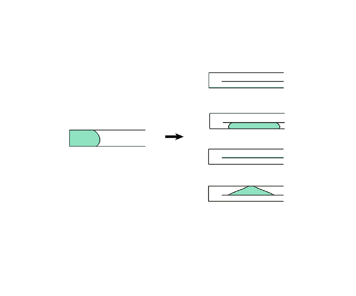

1. Introduction
Capillary plugs may occur due to the contribution of surface tension in a slit regardless of whether there is zero gravity or a transverse gravity field (de Gennes, Brochard-Wyart & Quéré Reference de Gennes, Brochard-Wyart and Quéré2004; Litterst et al. Reference Litterst, Eccarius, Hebling, Zengerle and Koltay2006; Zhang, Yang & Wang Reference Zhang, Yang and Wang2006). The characteristic lengths of the capillary plugging in the slit mainly range from millimetre to micron sizes. Some structures have been found to effectively address the occlusion problem when gravity can be neglected. For example, a corner with the angle smaller than
 $180^\circ -2\gamma$
for contact angle
 $\gamma \lt 90^\circ$
or 2
 $\gamma -180^\circ$
for
 $\gamma \gt 90^\circ$
can cause capillary non-occlusion (Concus & Finn Reference Concus and Finn1969). Compared with the zero-gravity condition, the gas–liquid interface becomes diversified for different transverse gravitational accelerations, determined by different Bond numbers (the Bond number measures the relative size of the gravitational force by comparison with the surface tension force on the liquid). Additionally, sometimes, there is a demand for shifting a liquid from a channel to another channel (e.g. vertically shifting, see Holló et al. Reference Holló, Suematsu, Ginder and Lagzi2021) in microfluidics.
For a horizontal channel in a downward gravity field, a larger size of the channel (corresponding to a larger Bond number) often has a weaker tendency to form the liquid plug according to physical common sense. This implies that the states of occlusion or non-occlusion can be related to the Bond number. Parry et al. (Reference Parry, Rascón, Jamie and Aarts2012) found that a change from capillary occlusion to non-occlusion occurred (the liquid spilled out through the openings) in the horizontal slit in a two-dimensional (2-D) planar condition as the Bond number increased beyond a critical value, and theoretically determined the critical Bond number line (i.e. the plot of the critical Bond number with respect to the contact angle).
The existence of a second solid structure (such as the rod) within a channel can enhance the performance of liquid transport, preventing the formation of occluding capillary surfaces. Such systems have been utilised in some industrial applications. For example, in the spacecraft liquid propellant tank, the vane-type propellant management device (PMD) is employed to control and transport the liquid propellants (Chen & Collicott Reference Chen and Collicott2004). The presence of the PMD creates a gap between the vane and the tank wall, which enables a capillary flow in a weightless environment. Besides, in some micro-injection pipettes (Oesterle Reference Oesterle2015), there exists a glass filament used for avoiding the air blockage and improving the liquid filling.
Inserting an object into a tubular channel at a central or eccentric position may cause the deformation of the interface (Finn Reference Finn1986; Elcrat, Kim & Treinen Reference Elcrat, Kim and Treinen2004; Gordon & Siegel, Reference Gordon and Siegel2010a ; Treinen Reference Treinen2012) and a change of the liquid state. Zhou et al. (Reference Zhou, Zhang, Zhu, Tan and Fu2021) theoretically and experimentally found that inserting a rod into a horizontal tube at the central position in a downward gravity field induced the change from liquid occlusion to non-occlusion in this tube for most cases. In zero gravity, eccentricity can result in capillary non-occlusion (Smedley Reference Smedley1990; Pour & Thiessen Reference Pour and Thiessen2019) due to the wetting effect (Parry, Rascón & Wood Reference Parry, Rascón and Wood2000). Eccentricity also can lead to capillary non-occlusion in a transverse body force field (Tan et al. Reference Tan, Zhou, Zhang, Zhu and Fu2022). In a horizontal eccentric annular tube, there are two mechanisms of capillary non-occlusion: the effect of a large enough transverse gravity and the wetting effect. These mechanisms lead to the existence of wetting-driven non-occlusion besides the transverse gravity-driven liquid non-occlusion and plug for different Bond numbers at a contact angle. This result is accompanied by two critical Bond number lines (each being in the form of a plot of critical Bond number as a function of contact angle). Crossing the upper critical Bond number line means a change between capillary plug and transverse gravity-driven non-occlusion. While, crossing the lower critical Bond number line illustrates the change between wetting-driven non-occlusion and a plug (Tan et al. Reference Tan, Zhou, Zhang, Zhu and Fu2022).
(a) Schematic of a gas–liquid interface in a 2-D horizontal plate-inserted slit in a downward gravity field in Cartesian coordinates (x, y). Here, H is the slit height, and
 $H_u$
and
 $H_l$
are the distances from the inserted plate to the upper and lower walls, i.e. the heights of the upper and lower channels, respectively. The liquid is situated at the left side of the gas–liquid interface, and the gas at the right side. The parameters
 $\gamma _1$
,
 $\gamma _2$
,
 $\gamma _3$
and
 $\gamma _4$
are the contact angles on the lower wall of the slit (contact point 1), the lower surface of the inserted plate (contact point 2), the upper surface of the inserted plate (contact point 3) and the upper wall of the slit (contact point 4), respectively. (b) Equilibrium Bond number for
 $\gamma _2 = 150^\circ$
,
 $\gamma _3 = 30^\circ$
and
 $H_l/H = 0.4$
versus contact angle
 $\gamma _1=\gamma _4$
. The upper (lower) inset shows that, when the Bond number is larger (smaller) than the equilibrium Bond number, the liquid loses the equilibrium and then flows into the lower (upper) channel.

In zero gravity, the shapes of liquid non-occluding interfaces in an eccentric annular tube are obtained by 2-D theoretical models (Pour & Thiessen Reference Pour and Thiessen2019). In a downward gravity field, the critical Bond numbers for the existence of liquid occlusion in a horizontal slit (Parry et al. Reference Parry, Rascón, Jamie and Aarts2012) or horizontal tubes (Manning, Collicott & Finn Reference Manning, Collicott and Finn2011; Rascón et al. Reference Rascón, Parry and Aarts2016; Zhou et al. Reference Zhou, Zhang, Zhu, Tan and Fu2021; Tan et al. Reference Tan, Zhou, Zhang, Zhu and Fu2022; Tan & Zhou Reference Tan and Zhou2024a ,Reference Tan and Zhou b ) are also determined based on 2-D theoretical models. The numerical data directly computed via the Surface Evolver code (Brakke Reference Brakke1992) in three-dimensional mode are used to validate the 2-D theoretical results in the case of zero gravity (Pour & Thiessen Reference Pour and Thiessen2019) or a transverse gravity (Manning et al. Reference Manning, Collicott and Finn2011; Rascón et al. Reference Rascón, Parry and Aarts2016; Zhou et al. Reference Zhou, Zhang, Zhu, Tan and Fu2021; Tan et al. Reference Tan, Zhou, Zhang, Zhu and Fu2022; Tan & Zhou Reference Tan and Zhou2024a ,Reference Tan and Zhou b ). Computational fluid dynamics (CFD) numerical methods have not been reported to be employed to determine the critical Bond numbers to date.
What is the effect of the insertion of a plate into a slit on the change of capillary state? Different from the case of a rod-inserted tube where all of the liquid is still in an annular channel, the two parts of liquid separated by the plate do not make contact in the vertical direction. Inserting a plate into a slit therefore has a different effect on the liquid state from that of inserting a rod into a tube at a central position (Zhou et al. Reference Zhou, Zhang, Zhu, Tan and Fu2021) or an eccentric position (Smedley Reference Smedley1990; Pour & Thiessen Reference Pour and Thiessen2019; Tan et al. Reference Tan, Zhou, Zhang, Zhu and Fu2022) regardless of whether there is zero gravity or transverse body forces. To figure out the effect of a plate insertion,
 $\S$
2 develops the formula describing the critical Bond numbers based on the energy minimisation and the nonlinear Young–Laplace equation in a 2-D planar condition and employs a CFD method to mutually verify the theoretical model. Section 3 investigates the capillary states of a droplet in the plate-inserted slit and examines the effects of the contact angles and the inserted plate’s position. Section 4 draws main conclusions from the analysis.
2. Method
2.1. Theoretical method
Consider a horizontal slit with the insertion of a horizontal plate (in reality, the end of the horizontal plate inside the slit is free but another end is fixed) in a downward gravity field. The length L and width W of the slit are far larger than the height H, and the thickness of the inserted plate is negligible. The gas–liquid interface is translationally invariant along the length of the slit. The liquid and the gas are immiscible and are assumed to have infinitely large volumes. Figure 1 shows the schematic of a gas–liquid interface within a horizontal plate-inserted slit in two dimensions, influenced by a downward gravity field in Cartesian coordinates (x, y). The origin of Cartesian coordinates is located on the lower wall of the slit. The horizontal position of the origin is not prescribed, because all of the equations in this section have translational invariance along the x direction. The forces acting on the liquid in the slit are the surface tension force and gravity. The Bond number measuring the relative size of the gravitational force by comparison with the surface tension force on the liquid is defined as
 \begin{equation} Bo = \frac {H^2}{l_{ca}^{2}}, \end{equation}
where the capillary length
 $l_{ca}$
is given by
 $l_{ca} = \sqrt {\sigma/{\rho g}}$
, where
 $\sigma$
is the surface tension between liquid and gas,
 $\rho$
is the density difference (positive) between liquid and gas and
 $g$
is the gravitational acceleration. The gas–liquid interface can be described by the Young–Laplace equation in a 2-D planar condition (Finn Reference Finn1986)
 \begin{equation} {\Bigg( {\frac {{{x_y}}}{{{\sqrt { {1 + x_y^2} }}}}} \Bigg)_{\!\!y}} = -(\sin \alpha )_y = \frac {y}{l_{ca}^{2}} + \lambda , \end{equation}
where y is the height of the interface,
 $\bullet _x$
and
 $\bullet _y$
denote the derivatives with respect to the coordinate x and y, respectively,
 $\alpha$
is the inclination angle of the interface to the y axis and is measured anticlockwise and
 $\lambda$
is a Lagrange parameter arising from the liquid volume. The parametrised form of (2.2) (Bhatnagar & Finn Reference Bhatnagar and Finn2016; Zhou & Zhang Reference Zhou and Zhang2017) is integrated to derive the solutions. The contact angle condition at each contact line (i.e. contact point in two dimensions) can be given by
 \begin{equation} \sin \alpha _i = \cos \gamma _i,\: \textrm {for} \: i = 1,3, \end{equation}
 \begin{equation} \sin \alpha _i = -\cos \gamma _i,\: \textrm {for} \: i = 2,4, \end{equation}
where
 $\gamma$
is the contact angle of the liquid on a solid surface, and the subscript i denotes the
 $i$
th contact point (i = 1, 2, 3 and 4 shown in figure 1
a). The effect of contact angle hysteresis is not taken into account. For the interface prescribed by (2.2) and (2.3a
,
b
), the total free energy of the corresponding liquid per unit width in a slit can be expressed as (Finn Reference Finn1986)
 \begin{equation} E = {E_I} + {E_W} + {E_G} + \sigma \lambda \Omega , \end{equation}
where
 $E_I$
is the interfacial energy,
 $E_W$
is the wetting energy,
 $E_G$
is the gravitational potential energy and
 $\Omega$
is the area of the liquid. For an equilibrium liquid as shown in figure 1, when a tiny horizontal displacement on the surface in the lower channel
 $\delta {x_l}$
occurs, another tiny horizontal displacement in the upper channel
 $\delta {x_u}$
in the opposite direction to
 $\delta {x_l}$
has to occur. The variation of energy from the equilibrium state before displacement to the equilibrium state after displacement is given by
 \begin{equation} \delta E = \delta {E_I} + \delta {E_W} + \delta {E_G} + \sigma \lambda \delta \Omega . \end{equation}
With invariant heights and contact angles of the lower channel and the upper channel, the shapes of the interfaces before and after displacement do not change. We have
 $|\Gamma _l| = |\Gamma _l^\prime |$
and
 $|\Gamma _u| = |\Gamma _u^\prime |$
, where
 $\Gamma _l$
and
 $\Gamma _u$
are denoted by the initial lower and upper interfaces, respectively, and
 $\Gamma _l^\prime$
and
 $\Gamma _u^\prime$
by the ones after displacement, respectively. In this case, we obtain
 \begin{equation} \delta {E_I} = 0. \end{equation}
The total volume (area in two dimensions) of the liquid remains constant. The variations of the liquid area in the lower and upper channels are
 $\delta \Omega _l = H_l\delta x_l$
and
 $\delta \Omega _u = H_u\delta x_u$
, respectively. The heights of the centres of
 $\delta \Omega _l$
and
 $\delta \Omega _u$
are
 $ ({1}/{2}) H_l$
and
 $H_l + ({1}/{2})H_u$
, respectively. Thus the variation of the gravitational potential energy
 $E_G$
can be given by
 \begin{equation} \delta {E_G} = \rho g\bigl( {\tfrac {1}{2}{H_l}^2\delta {x_l} + \bigl( {{H_l} + \tfrac {1}{2}{H_u}} \bigr){H_u}\delta {x_u}} \bigr). \end{equation}
The horizontal displacement
 $\delta x_l$
of the interface in the lower channel leads to the same displacement at the contact points 1 and 2 (see figure 1
a), which results in the variation of the wetting energy of the walls of the lower channel being
 $-\sigma \cos\gamma _1 x_l-\sigma \cos \gamma _2 \delta x_l$
. Similarly, the variation of the wetting energy of the walls of the upper channel is
 $-\sigma \cos\gamma _2 x_u-\sigma \cos \gamma _3 \delta x_u$
. The variation of the wetting energy
 $E_W$
can therefore be expressed as
 \begin{equation} \delta {E_W} = - \sigma \left ( {\cos {\gamma _1} + \cos {\gamma _2}} \right )\delta {x_l} - \sigma \left ( {\cos {\gamma _3} + \cos {\gamma _4}} \right )\delta {x_u}. \end{equation}
Since the liquid bulk conserves its volume (area in two dimensions), we have the following relationship:
 \begin{equation} \delta \Omega = \delta \Omega _l + \delta \Omega _u = {H_l}\delta {x_l} + {H_u}\delta {x_u} = 0. \end{equation}
Substituting (2.6)–(2.9) into (2.5), the equilibrium Bond number
 $Bo_e$
is obtained as
 \begin{equation} B{o_e} = - \frac {{2H}}{{{H_l}}}\left ( {\cos {\gamma _1} + \cos {\gamma _2}} \right ) + \frac {{2H}}{{{H_u}}}\left ( {\cos {\gamma _3} + \cos {\gamma _4}} \right ). \end{equation}
Only when
 $Bo=B{o_e}$
can the interfaces be in both lower and upper channels and be in equilibrium at the same time. If
 $Bo\gt B{o_e}$
, then
 $\delta E\lt 0$
and all of the liquid enters the lower channel. If
 $Bo\lt B{o_e}$
, then
 $\delta E\gt 0$
and all of the liquid enters the upper channel. Notably, the value of (2.10) will be negative for some contact angles. In this situation, the equilibrium Bond number
 $Bo_e$
does not exist in reality, and the liquid is in the lower channel for any Bond number.
Once all the liquid enters the lower (upper) channel, the liquid will either occlude or not occlude the lower (upper) channel. Take the lower channel as an example. By integrating the parametrised form of the Young–Laplace equation (2.2) with respect to the coordinate y and applying the contact angle condition (2.3), we can obtain
 \begin{equation} \sin \alpha = \frac {1}{2} \frac {y^2}{l^{2}_{ca}} + \lambda y - \cos \gamma _1, \end{equation}
 \begin{align} \lambda = \frac {\cos \gamma _1 + \cos \gamma _2}{H_l} - \frac {1}{2} \frac {H_l^2}{l^{2}_{ca}}. \\[6pt] \nonumber \end{align}
Under a downward gravitational field, the occluding configuration, as shown in figure 2, reaches its limit when the length of the interface along the x-direction approaches infinity (considering the condition of infinite liquid). In this limiting situation, the interface is expected to be nearly parallel to the x-direction, satisfying
 \begin{equation} \min (\sin \alpha ) = \min \left(\frac {1}{2} \frac {y^2}{l^{2}_{ca}} + \lambda y - \cos \gamma _1\right) = -1. \end{equation}
In (2.13), the minimum value of (
 $({1}/{2}) y^2 l^{-2}_{ca} + \lambda y - \cos \gamma _1$
) is reached when
 $(\textrm {d}/\textrm {d}y)(({1}/{2}) y^2 l^{-2}_{ca} + \lambda y - \cos \gamma _1) = 0$
and the corresponding value of
 $y$
is
 $-\lambda l^2_{ca}$
. Based on (2.12) and (2.13), we have
 \begin{equation} \frac {H_l^2}{l_{ca}^2} = 4 \left ( \textrm {sin}\frac {\gamma _1}{2} + \textrm {cos}\frac {\gamma _2}{2}\right )^2, \end{equation}
or
 \begin{equation} \frac {H_l^2}{l_{ca}^2} = 4 \left ( \textrm {sin}\frac {\gamma _1}{2} - \textrm {cos}\frac {\gamma _2}{2}\right )^2. \end{equation}
However, when the relation (2.14b
) is satisfied, it is found that
 $y = -\lambda l_{ca}^2 \notin [0, H_l]$
, suggesting that the parallel (to the x-direction) part of the interface is outside the lower channel, and thus, the corresponding limiting situation is non-physical. Therefore, only the relation (2.14a
) identifies the limiting situation of the occluding liquid in the lower channel. The critical Bond number
 $Bo_{cl}$
of liquid non-occlusion in the lower channel is defined as the Bond number satisfying the relation (2.14a
). According to the definition of Bond number (2.1) and the relation (2.14a
), we can obtain
 $Bo_{cl}$
as
 \begin{equation} B{o_{cl}} =\frac {H^2}{l_{ca}^2} =\left [\frac {2H}{H_l} \left (\sin \frac {\gamma _1}{2} + \cos \frac {\gamma _2}{2}\right ) \right ]^2. \end{equation}
Equation (2.15) is based on the definition (2.1) of the Bond number. Similarly, the critical Bond number
 $Bo_{cu}$
of liquid non-occlusion in the upper channel is
 \begin{equation} B{o_{cu}} =\frac {H^2}{l_{ca}^2} = \left [\frac {2H}{H_u} \left (\sin \frac {\gamma _3}{2} + \cos \frac {\gamma _4}{2}\right ) \right ]^2. \end{equation}
In other words, instead of the height of the lower or upper channel, the height of the slit is used as the characteristic length scale under the context of (2.15). Or else, three different characteristic length scales will lead to non-comparability of (critical) Bond numbers. Equations (2.15) and (2.16) are used to calculate the critical Bond numbers for the lower and upper channels, respectively. For an open slit (without an inserted plate), the critical Bond number for the liquid non-occlusion can be obtained in the same way and is given by
 \begin{equation} B{o_{cs}} = 4 \left (\sin \frac {\gamma _1}{2} + \cos \frac {\gamma _4}{2}\right )^2. \end{equation}
This expression (2.17) of the critical Bond number is equivalent to that developed from the Kelvin equation by Parry et al. (Reference Parry, Rascón, Jamie and Aarts2012). The critical Bond numbers for different liquid volumes and different contact angles calculated using the theoretical model are found to agree well with the data directly computed via Surface Evolver (Brakke Reference Brakke1992) in 2-D mode (figure 3 b). This fully demonstrates the validity of the theoretical model.
Schematic of the evolution of the interface for infinite liquid in a horizonal channel in two dimensions as the Bond number gradually increases (from left to right) and approaches the critical Bond number.

(a) Schematic of a gas–liquid interface in the lower channel of the plate-inserted slit and (b) the ratio of the critical Bond number for finite liquid to the critical Bond number for infinitely large liquid (
 $Bo^*_{cl}/Bo_{cl}$
) versus the liquid area relative to the square of the height of the lower channel. Here,
 $\Omega _l$
is the area of liquid in the lower channel. In (b), different curves theoretically calculated for
 $\gamma _1 = \gamma _2 = 60^\circ , 90^\circ$
and
 $120^\circ$
are shown, while the crosses (
 $\times$
) denote the data directly computed via Surface Evolver (Brakke Reference Brakke1992) in 2-D mode. The squares (
 $\square$
) denote the representative points each corresponding to a cross-section of the liquid at a critical Bond number. Here, A and B correspond to
 $Bo^*_{cl}/Bo_{cl} =$
0.4 and 0.99, respectively, for
 $\gamma _1 = \gamma _2 = 60^\circ$
, while C and D correspond to
 $Bo^*_{cl}/Bo_{cl} =$
0.4 and 0.99, respectively, for
 $\gamma _1 = \gamma _2 = 120^\circ$
.

The expression (2.15) of the critical Bond number is developed by assuming an infinite area of the liquid, as shown in figure 3(
 $a$
). The liquid area (
 $\Omega _l$
) has a certain effect on the critical Bond numbers, as the interface does not extend infinitely. The left and the right parts of the interface coming into contact with each other (as seen the insets A–D in figure 3
b) is expected to lead to the disappearance of the occlusion, which is regarded as the limiting situation under a finite liquid. Suppose the liquid occludes the lower channel. For a given Bond number, we determine the right part of the interface by directly solving the Young–Laplace equation (2.2), and obtain the left part by mirroring the right part. For the limiting situation of the left and the right parts of the interface just touching each other, the liquid area (
 $\Omega _l$
) surrounded by the interface and the walls can be obtained. Then, the value of the given Bond number is identified as the critical Bond number (
 $Bo^*_{cl}$
) for the finite liquid area
 $\Omega _l$
. Figure 3(b) shows the variations of the ratio of the critical Bond number for finite liquid (
 $Bo^*_{cl}$
) to the critical Bond number for infinitely large liquid (
 $Bo_{cl}$
) for different contact angles with the area of liquid relative to the square of the height of the lower channel (
 $\Omega _l/H_l^2$
). The results show that the critical Bond number decreases with larger contact angle for a liquid with a non-small area. The critical Bond numbers approximate that of an infinitely large liquid, when the liquid area is large enough (
 $\geqslant H_l^2$
for
 $\gamma _1=\gamma _2=60^\circ$
,
 $\geqslant 1.2 H_l^2$
for
 $\gamma _1=\gamma _2=90^\circ$
and
 $\geqslant 1.5 H_l^2$
for
 $\gamma _1=\gamma _2=120^\circ$
). Such a large liquid area is easy to reach in practical microfluidics. Accordingly, the analysis in the following sections will be conducted based on the assumption of an infinitely large liquid and the effect of the liquid volume will not be considered.
2.2. Computational fluid dynamics method
The numerical simulations of the evolution of the gas–liquid interface in the slit–plate structure are based on a CFD method using COMSOL Multiphysics 5.6. Considering an immiscible liquid and gas, we couple two methods (i.e. laminar flow method and the phase field method) to describe the laminar incompressible flow and track the movement of the interface. According to Cahn & Hilliard (Reference Cahn and Hilliard1958), the chemical potential
 $G$
is expressed by the mixing of two phases as
 \begin{equation} G = \zeta \left [-{\nabla }^2{\phi } + \frac {(\phi ^2-1)\phi }{\epsilon ^2}\right ]= \frac {\zeta }{\epsilon ^2}\psi , \end{equation}
 \begin{align} \psi = -{\nabla } \cdot {\epsilon ^2}{\nabla }{\phi } + (\phi ^2-1)\phi , \\[6pt] \nonumber \end{align}
where
 $\zeta$
is the chemical potential density,
 $\epsilon$
is the interface thickness parameter and
 $\phi$
is the phase field variable representing the interfacial layer. In the phase field method, the transition area of the phase is defined as the variation of
 $\phi$
from
 $-1$
to
 $+1$
. The heavy liquid and light gas correspond to
 $+1$
and
 $-1$
, respectively. In addition, the chemical potential density
 $\zeta$
and the interface thickness parameter
 $\epsilon$
are related to the surface tension
 $\sigma$
by
 \begin{equation} \sigma = \frac {2\sqrt {2}}{3}\frac {\zeta }{\epsilon }. \end{equation}
The flow is described by the incompressible Navier–Stokes equations
 \begin{equation} \rho \left(\frac {{\partial {\boldsymbol {u}}}}{{\partial t}} + \boldsymbol {u} \cdot \nabla \boldsymbol {u} \right) = \nabla \cdot \left [ { - p {\unicode{x1D644}} + \mu \left ( {\nabla \boldsymbol {u} + (\nabla {{\boldsymbol {u}})^{\text T}}} \right )} \right ] + G\nabla \phi + \rho \boldsymbol {g}, \end{equation}
 \begin{equation} \nabla \cdot \boldsymbol {u} = 0, \end{equation}
where the velocity vector
 $\boldsymbol {u}$
= (
 $u$
,
 $v$
),
 $p$
is the fluid pressure,
 $\mu$
is the fluid dynamic viscosity and
 $\boldsymbol {g}=(0,-g)$
indicates that gravity is in the
 $-y$
direction. The force of the flow field acting on the interface is modelled by the Cahn–Hilliard equation
 \begin{equation} \frac {\partial \phi }{\partial t} + \boldsymbol {u}\cdot \nabla \phi = \nabla \cdot \left (\Gamma \nabla G\right ), \end{equation}
where
 $\Gamma$
is the mobility. The fluid density
 $\rho$
and fluid dynamic viscosity
 $\mu$
in the phase filed method are governed by the phase field variable
 $\phi$
, expressed as
 \begin{equation} \rho = {\rho }_l {\eta }_l + {\rho }_{g} {\eta }_{g}, \end{equation}
 \begin{equation} \mu = {\mu }_{l} {\eta }_{l}+ {\mu }_{g} {\eta }_{g}, \end{equation}
 \begin{equation} \eta _l = \frac {1 - \phi }{2},\quad \eta _g = \frac {1 + \phi }{2}, \end{equation}
where the subscripts
 $l$
and
 $g$
represent liquid and gas, respectively, and
 $\eta$
denotes the volume fraction of liquid or gas in a cell in numerical simulation.
A rectangular domain is generated for simulating a horizontal slit with an inserted plate partially submerged in liquid. This configuration features a structure that contains an inserted plate with a negligible thickness to simulate the movement of liquid within the slit (figure 4). All walls adhere to the no-slip boundary condition, and the exit is an open boundary. The main simulation parameters are given in table 1. One end of the plate is submerged in liquid at the initial state. The multifrontal massively parallel sparse direct solver (MUMPS) is suitable for linear equations with arbitrary symmetry, and the robustness of the solution is increased by partial principal element elimination. The MUMPS method is used to solve the time-dependent problem. The calculated results for different grid numbers (i.e.
 $N = 16\,846$
, 41 496 and 1 26 377) of triangular grids are compared, and the
 $x$
values of the contact points at different times for
 $N = 41\,496$
remain nearly equal to those for
 $N = 1\,26\,377$
(see figure 5). Therefore, the triangular mesh method with the number of grids at
 $N =$
41 496 (the corresponding minimum element size
 $S_{min} = 0.15$
μm) is used.
Schematic of the computational domain for CFD numerical simulation on the fluids in a plate-inserted slit at the initial state. The green part represents the liquid, while the remaining area denotes the gas.

Values of main parameters of the simulations.

In the CFD numerical simulations, different Bond number conditions are achieved by changing the value of gravitational acceleration. The parameter
 $\epsilon = 0.5S_{max}$
, controlling the interface thickness, is proportional to the maximum element size
 $S_{max}$
. The mobility tuning parameter
 $\chi$
determines the mobility
 $\Gamma$
. The mobility controlled by both the interface thickness and the mobility tuning parameter is given by
 \begin{equation} \Gamma = \chi \epsilon ^2, \end{equation}
 \begin{equation} \chi = \frac {2 |\boldsymbol {u}|_{max}}{3\sqrt {2}\sigma } \frac {S_{max}}{\epsilon }. \end{equation}
The initial velocities of the fluids are set to zero.
Grid independence test of CFD numerical simulations with
 $\gamma _1 = \gamma _2 =\gamma _3 = \gamma _4 = 90^\circ$
and
 $Bo = 7$
for different grid numbers. Here,
 $x$
represents the
 $x$
-value of the contact point on the bottom surface of the lower channel at a moment t.

Equilibrium Bond number and critical Bond numbers for
 $\gamma _2=150^\circ$
,
 $\gamma _3=30^\circ$
and
 $H_l/H = 0.4$
versus contact angle
 $\gamma _1=\gamma _4$
. The green curve denotes the critical Bond number (
 $Bo_{cs}$
) for an open slit without a plate inserted. The black curve denotes the equilibrium Bond number (
 $Bo_{e}$
) for the plate-inserted slit. The red and blue curves denote the critical Bond numbers (
 $Bo_{cl}$
and
 $Bo_{cu}$
) of the lower and upper channels, respectively. The dark (light) blue region denotes state A (B), i.e. liquid occlusion (non-occlusion) in the upper channel. The dark (light) brown region denotes state C (D), i.e. liquid occlusion (non-occlusion) in the lower channel. The points
 $P_1$
,
 $P_2$
,
 $P_3$
and
 $P_4$
corresponding to
 $Bo=$
1.5, 5, 20 and 39 at
 $\gamma _1=\gamma _4=150^\circ$
denote the representative cases of states A, B, C and D, respectively, and their liquid configurations are schematically shown on the right side. Triangles, pluses, stars and squares denote the CFD numerical results in states
 $A$
,
 $B$
,
 $C$
and
 $D$
, respectively.

3. Multiple states of liquid
In this section, the results of typical cases calculated using the theoretical model are presented, illustrating various states of liquid in a slit with an inserted plate under different conditions of contact angles and plate positions. The numerical results based on the CFD method are also given, demonstrating good agreement with the theoretical predictions.
3.1. Observation of multiple states of liquid
Taking the case of
 $\gamma _2=150^\circ$
,
 $\gamma _3=30^\circ$
and
 $H_l/H =$
0.4 as an example, the variations of the equilibrium Bond number and the critical Bond numbers with the contact angle
 $\gamma _1 = \gamma _4$
are shown in figure 6. Different from the insertion of a rod into a tube at a central or eccentric position only causing non-occlusion in some cases, the insertion of a plate at an arbitrary position can lead to at least one non-occluded gas passage in the slit in all cases except for an extreme case where the droplet occludes both the lower and upper channels (see the equilibrium Bond number points on the black curve in figure 6). The liquid states are different from those in horizontal rod-inserted tubes (Tan et al. Reference Tan, Zhou, Zhang, Zhu and Fu2022). We observe the existence of four types of liquid states, i.e. liquid plugs in the upper channel (state A, see point
 $P_1$
), liquid non-occlusion in the upper channel (state B, see point
 $P_2$
), liquid plugs in the lower channel (state C, see point
 $P_3$
) and liquid non-occlusion in lower channel (state D, see point
 $P_4$
).
As shown in figure 6, for state A, the liquid occlusion in the upper channel is accompanied by liquid non-occlusion in the lower channel. For state B, the liquid non-occlusion in the upper channel is accompanied by the drainage through the upper exit, and the liquid drainage back to the slit or into the lower channel occurs with difficulty in the current slit structure (figure 1) under the effect of fluid inertia in practice. For state C, the liquid plug in the lower channel is accompanied by liquid non-occlusion in the upper channel. For state D, the liquid non-occlusion in the lower channel is fully non-occluding theoretically. State A (C) demonstrates that liquid flows to the upper (lower) channel, which could help to control the vertically shifting direction of liquid in small channels.
Note that, without the inserted plate, the liquid non-occlusion can be achieved in an open slit when the Bond numbers are larger than the corresponding critical Bond numbers
 $Bo_{cs}$
(denoted by the green curve in figure 6) theoretically calculated from (2.17). The existence of state B or D below the green curve indicates the applicability of the insertion of a plate for removing the liquid in a liquid-plugged slit.
3.2. Numerical validation
The numerical calculation on the fluids in the slit–plate structure is conducted based on the CFD method described in
 $\S$
2.2. Figure 7(
 $a$
–
 $d$
) presents the simulation results of the liquid evolution for the representative cases of four types of liquid states, which correspond to the points
 $P_1$
,
 $P_2$
,
 $P_3$
and
 $P_4$
in figure 6, respectively. For the cases shown in figure 7(
 $a$
,
 $c$
), the majority of the liquid can eventually reach a steady state and occlude a channel after a certain computational moment, while some other parts may flow out of the simulation domain through the open boundary (on the right side of the slit) or remain attached to the channel wall (see, e.g. the liquid on the plate as shown in figure 7
 $c$
). In addition, the numerical results for the gas–liquid interfaces of the occluding parts exhibit a shape similarity to the theoretical results. For the cases shown in figure 7(
 $b$
,
 $d$
), the majority of the liquid flows out, while some parts remain in the channel. The above numerical results validate the theoretical predictions (as shown by the liquid configurations of
 $P_1$
,
 $P_2$
,
 $P_3$
and
 $P_4$
in figure 6) regarding the liquid states, except for the minor portion of the liquid which does not compromise the overall significance.
Computational fluid dynamics numerical simulation of the liquid evolution in the plate-inserted slit (
 $\gamma _1 =\gamma _2 = \gamma _4 = 150^\circ$
,
 $\gamma _3 = 30^\circ$
and
 $H_l/H =$
0.4) for (a)
 $Bo = 1.5$
, (b)
 $Bo = 5$
, (c)
 $Bo = 20$
and (d)
 $Bo = 39$
. The cases (a), (b), (c) and (d) correspond to the points
 $P_1$
,
 $P_2$
,
 $P_3$
and
 $P_4$
in figure 6, respectively. The calculation is terminated when the majority of the liquid reaches a steady state or when the majority of the liquid flows out through the exit. Each row presents the results at different computing moments, i.e. the initial moment, an intermediate moment and the termination moment. Each panel has a display range of
 $x$
coordinate from 0 to 5 mm except the third panel of (
 $c$
) whose display range is from 3 to 8 mm.

As shown in figure 6, more numerical results for the liquid states (denoted by the different symbols) are presented, which are in good agreement with the theoretical results. Notably, the theoretical equilibrium at the equilibrium Bond number (corresponding to the black curve in figure 6) is unattainable in the numerical simulation, because any small deviation (which can be induced by the numerical error) in the exact conditions of Bond number or contact angle will break the equilibrium.
4. Results and discussion
Non-uniformity of the contact angles on different walls always greatly influences the capillary plugs and non-occlusion in a slit (Parry et al. Reference Parry, Rascón, Jamie and Aarts2012) or a tube (Verma et al. Reference Verma, Saraj, Yadav, Singh and Guo2020; Zhu, Zhou & Zhang Reference Zhu, Zhou and Zhang2020). For the slit–plate structure considered in this study, the contact angles on different walls (including
 $\gamma _1$
,
 $\gamma _2$
,
 $\gamma _3$
and
 $\gamma _4$
) are important factors influencing the equilibrium Bond number and the critical Bond numbers. In this section, we comprehensively investigate the effect of contact angle conditions on the liquid state. The aim of this paper is to study the capacity of removing the liquid plug in a horizontal slit and, in reality, the contact angles on the upper and lower walls of an existing liquid-plugged slit often do not show much difference. Accordingly, only the situation of
 $\gamma _1 = \gamma _4$
is considered here. The contact angle of
 $\gamma _1 = \gamma _4$
studied here ranges from
 $0^\circ$
to
 $180^\circ$
at intervals of
 $1^\circ$
. We also examine the influence of the position of the plate, which is another crucial factor.
4.1. Equal contact angles on slit and plate surfaces
Consider equal contact angles of the slit walls and the two surfaces of the inserted plate (
 $\gamma =$
 $\gamma _1=\gamma _2=\gamma _3=\gamma _4$
). In this case, for either the upper or lower channel, the capillary effect tends to attract the liquid into the channel under the hydrophilic condition (
 $\gamma \lt 90^\circ$
) while it tends to exclude the liquid out under the hydrophobic condition (
 $\gamma \gt 90^\circ$
). There always exists a competition between the capillary effects induced by the upper and lower channels to place the liquid. Hence, the position of the plate plays an important role in determining the liquid state, and the narrower channel is expected to have a stronger capillary effect. When the plate is near the lower wall of the slit (e.g. the case depicted in figure 8
a), the lower channel has a stronger capillary effect on the liquid. Thus, for
 $\gamma \lt 90^\circ$
, the total capillary force as well as the downward gravity will pull the liquid into the lower channel, and the liquid equilibrium cannot occur in the upper channel. As a result, the equilibrium Bond numbers (corresponding to the black curve) along with state
 $A$
or
 $B$
do not exist for
 $\gamma \lt 90^\circ$
, as shown in figure 8(
 $a$
). For
 $\gamma \gt 90^\circ$
, state
 $A$
(the dark blue region in figure 8
 $a$
) can occur for some smaller Bond numbers (below the equilibrium Bond numbers) because the total capillary force can overcome the downward gravity and pull the liquid into the upper channel. Conversely, when the plate is near the upper wall of the slit (e.g. the case depicted in figure 8
b), the upper channel has a stronger capillary effect and thus, the equilibrium Bond numbers exist for
 $\gamma \lt 90^\circ$
and state
 $A$
can occur below the equilibrium Bond numbers.
In such a situation, however, liquid non-occlusion always occurs in the lower channel (i.e. state
 $D$
) and the corresponding critical Bond numbers are always larger than those of an open slit without an inserted plate (i.e. the red curves are above the green curves, as shown in figure 8
a,b). The simple reason for this is that a narrower channel would require a larger downward gravity for non-occlusion, which can be inferred from (2.15)–(2.17). This also implies that the insertion of a plate into a liquid-plugged slit with the same contact angle does not contribute to the liquid removal.
Equilibrium Bond number and critical Bond numbers versus contact angle (
 $\gamma =\gamma _1=\gamma _4=\gamma _2=\gamma _3$
) for (a)
 $H_l/H = 0.4$
and (b)
 $H_l/H = 0.6$
. The green curve denotes the critical Bond number (
 $Bo_{cs}$
) of an open slit without a plate inserted. The black curve denotes the equilibrium Bond number (
 $Bo_{e}$
) of the plate-inserted slit. The red and blue curves denote the critical Bond numbers (
 $Bo_{cl}$
and
 $Bo_{cu}$
) of the lower and upper channels, respectively. The blue region denotes state A, i.e. liquid occlusion in the upper channel. The dark (light) brown region denotes state C (D), i.e. liquid occlusion (non-occlusion) in the lower channel. Note that state
 $B$
(i.e. liquid non-occlusion in the upper channel) does not exist for the presented cases.

4.2. Equal contact angles on the plate’s lower and upper surfaces
Consider a scenario where the contact angles on the inserted plate’s lower and upper surfaces are equal (
 $\gamma _2 = \gamma _3$
). Figure 9 shows the variations of the equilibrium Bond number and the critical Bond numbers for different plate contact angles and different plate positions with
 $\gamma _1 = \gamma _4$
. Due to the similar wetting conditions on the upper and lower channels (i.e.
 $\gamma _1 = \gamma _4$
and
 $\gamma _2 = \gamma _3$
), there is a competition between the two channels for liquid placement. When the plate is near the lower (upper) wall of the slit, the equilibrium Bond number does not exist for
 $\gamma _1 = \gamma _4 \lt 90^\circ$
and
 $\gamma _2 = \gamma _3 \lt 90^\circ$
(
 $\gamma _1 = \gamma _4 \gt 90^\circ$
and
 $\gamma _2 = \gamma _3 \gt 90^\circ$
), as shown in figure 9. It is also found that, for a single channel (the upper or lower channel), the increase (decrease) of the contact angle on the upper (lower) wall of the channel can reduce the critical Bond number of the channel. This is because that the liquid in a (upper or lower) channel tends to move away from the upper wall with a larger contact angle and towards the lower wall with a smaller contact angle, making the downward gravity more effective in pulling the liquid down and preventing occlusion.
The liquid removal from the slit for the cases shown in figure 9(
 $a$
–
 $c$
) mainly depends on state
 $B$
(since state
 $D$
exists for these cases at very large Bond numbers and is not shown in figure 9
 $a$
–
 $c$
), whereas the non-occlusion for the cases shown in figure 9(
 $d$
–
 $f$
) depends on state
 $D$
. The region of state
 $B$
below the critical Bond numbers of the open slit (the green curve) and the corresponding contact angle range of the slit walls (
 $\gamma _1 = \gamma _4$
) reach the global peak value under the condition of
 $\gamma _2 = \gamma _3=$
 $90^\circ$
when the plate contact angles gradually increase (see, e.g. figure 9
 $a$
–
 $c$
). The peak value indicates a maximum contact angle range of the slit walls that is applicable to liquid removal at a given
 $H_l/H$
. The region of state
 $D$
below the green curve and the corresponding contact angle range of the slit walls increase with the increase of the plate contact angles (see figure 9
 $d$
–
 $f$
). The region for state
 $B$
below the green curve appearing at
 $\gamma _1 = \gamma _4$
larger than approximately
 $150^\circ$
for the cases in figure 9(
 $a$
–
 $c$
) suggests that a hydrophilic inserted plate is applicable for removing the liquid in the open slit with superhydrophobic walls. Conversely, the hydrophobic inserted plate can be effective when the open slit’s walls have not-so-large contact angles, as indicated by the region for state
 $D$
below the green curve shown in figure 9(
 $f$
).
Equilibrium Bond number and critical Bond numbers versus
 $\gamma _1=\gamma _4$
for equal plate contact angles (
 $\gamma _2=\gamma _3$
) of (
 $a$
)
 $60^\circ$
, (
 $b$
)
 $90^\circ$
and (
 $c$
)
 $120^\circ$
at
 $H_l/H =$
0.2, and (
 $d$
)
 $91^\circ$
, (
 $e$
)
 $120^\circ$
and (
 $f$
)
 $150^\circ$
at
 $H_l/H=$
0.8. The green curve denotes the critical Bond number (
 $Bo_{cs}$
) of an open slit without a plate inserted. The black curve denotes the equilibrium Bond number (
 $Bo_{e}$
) of the plate-inserted slit. The red and blue curves denote the critical Bond numbers (
 $Bo_{cl}$
and
 $Bo_{cu}$
) of the lower and upper channels, respectively. The dark (light) blue region denotes state A (B), i.e. liquid occlusion (non-occlusion) in the upper channel. The dark (light) brown region denotes state C (D), i.e. liquid occlusion (non-occlusion) in the lower channel.

The contact angle range of the slit walls (
 $\gamma _1 = \gamma _4$
) for state
 $B$
(state
 $D$
) below the critical Bond numbers of the open slit indicates the application coverage of the inserted plate for liquid removal through the upper (lower) channel. From figure 10(
 $a$
–
 $c$
), it is found that, for the liquid removal through the upper channel, the optimal condition for the plate contact angles
 $\gamma _2 = \gamma _3$
is near
 $90^\circ$
for different values of
 $H_l/H$
(e.g.
 $91^\circ$
for
 $H_l/H = 0.1$
and
 $90^\circ$
for
 $H_l/H = 0.2, 0.26, 0.27, 0.28$
and
 $0.29$
). Furthermore, a larger
 $H_l/H$
corresponds to a smaller application coverage on liquid removal for a given plate contact angle (
 $\gamma _2 = \gamma _3$
), and when
 $H_l/H$
is larger than approximately the critical value, the liquid removal cannot occur regardless of the slit wall contact angles (
 $\gamma _1 = \gamma _4$
). The critical value of
 $H_l/H$
is approximately equal to 0.29 at the peak plate contact angles
 $\gamma _2 = \gamma _3 = 90^\circ$
(see figure 10
b). The critical value of
 $H_l/H$
is approximately equal to or slightly smaller than 0.29, except for the cases at very small contact angles and sufficiently large contact angles (see figure 10
a–c). Regarding the liquid removal through the lower channel, it cannot occur when the plate contact angle (
 $\gamma _2 = \gamma _3$
) is not larger than
 $90^\circ$
, and as shown in figure 10(
 $d$
–
 $f$
), a larger value of
 $\gamma _2 = \gamma _3$
contributes to a greater applicability. In addition, a larger
 $H_l/H$
often corresponds to a greater application coverage on liquid removal through the lower channel except for some cases such as
 $\gamma _2 = \gamma _3 = 120^\circ$
with
 $H_l/H$
approaching 1 (see figure 10
 $e$
).
Contact angle range of the slit walls (
 $\gamma _1 = \gamma _4$
) for state
 $B$
((a)
 $60^\circ$
, (b)
 $90^\circ$
and (c)
 $120^\circ$
) and state
 $D$
((d)
 $91^\circ$
, (e)
 $120^\circ$
and (f)
 $150^\circ$
) below the open slit’s critical Bond numbers for different plate positions at equal plate contact angles (
 $\gamma _2 = \gamma _3$
). The insets in (b,e) show the widths of the slit’s contact angle range (
 $\Delta \gamma$
) for state
 $B$
and state
 $D$
below the open slit’s critical Bond numbers as a function of
 $\gamma _2 = \gamma _3$
for different values of
 $H_l/H$
, respectively.

4.3. Complementary contact angles on the plate’s lower and upper surfaces
The situation of different wetting conditions on the lower and upper surfaces of the plate is considered for the slit–plate system, taking the complementary contact angles (
 $\gamma _2 = 180^\circ - \gamma _3$
) as an example. The phase diagrams of two representative cases (
 $\gamma _2 = 180^\circ - \gamma _3=150^\circ$
and
 $\gamma _2 = 180^\circ - \gamma _3=30^\circ$
) with varying slit wall contact angle (
 $\gamma _1=\gamma _4$
) and Bond number are shown in figure 11(
 $a$
,
 $b$
). Notably, the cases in figures 11(
 $a$
) and 11(
 $b$
) can be obtained by altering the contact angles of the lower plate surface in figures 9(
 $a$
) and 9(
 $f$
), respectively.
Equilibrium Bond number and critical Bond numbers versus
 $\gamma _1=\gamma _4$
for (
 $a$
)
 $\gamma _2=150^\circ$
,
 $\gamma _3=30^\circ$
at
 $H_l/H=$
0.2, and (
 $b$
)
 $\gamma _2=30^\circ$
,
 $\gamma _3=150^\circ$
at
 $H_l/H=$
0.8. The green curve denotes the critical Bond number (
 $Bo_{cs}$
) of an open slit without a plate inserted. The black curve denotes the equilibrium Bond number (
 $Bo_{e}$
) of the plate-inserted slit. The red and blue curves denote the critical Bond numbers (
 $Bo_{cl}$
and
 $Bo_{cu}$
) of the lower and upper channels, respectively. The dark (light) blue region denotes state A (B), i.e. liquid occlusion (non-occlusion) in the upper channel. The dark (light) brown region denotes state C (D), i.e. liquid occlusion (non-occlusion) in the lower channel.

For the case shown in figure 11(
 $a$
), since
 $\gamma _1=\gamma _4$
and
 $\gamma _2\gt \gamma _3$
 $=180^\circ - \gamma _2$
, the upper channel can have a stronger wetting effect than the lower channel, which overcomes the downward gravity effect to attract the liquid into the upper channel. Therefore, compared with the case shown in figure 9(
 $a$
), the scenario depicted in figure 11(
 $a$
) exhibits a significantly larger total region of states
 $A$
and
 $B$
(representing the situation of liquid entering the upper channel), as well as a notably larger region of state
 $B$
below the critical Bond numbers of the open slit (the green curve) covering a wider slit wall contact angle range from approximately
 $65^\circ$
to
 $180^\circ$
. This suggests that the inserted plate with the lower hydrophobic surface and the upper hydrophilic surface is superior to the plate with lower and upper uniformly hydrophilic surfaces in terms of removing liquid, primarily for removing the liquid plug existing in the slit with large contact angles on the walls.
For the case shown in figure 11(
 $b$
), the values of equilibrium Bond number for any contact angle (
 $\gamma _1=\gamma _4$
) are less than zero (and are thus not shown), indicating that the liquid cannot enter the upper channel against downward gravity. Although the total region of states
 $C$
and
 $D$
occupies the entire space of two parameters (i.e. slit wall contact angle and Bond number), the region of state
 $D$
below the green curve does not exist. This implies that the inserted plate is not applicable for removing the liquid in the slit in these cases. From figures 9(
 $d$
–
 $f$
) and 11(
 $b$
), a necessary condition for the existence of the part of the region of state
 $D$
below the green curve is given by the inequality
 $Bo_{cs} \gt {max}(Bo_{cl}, Bo_e)$
. However, this inequality cannot hold under the wetting conditions of
 $\gamma _1=\gamma _4$
and
 $\gamma _2 = 180^\circ - \gamma _3$
, regardless of
 $H_l/H$
, as can be easily proven according to (2.10), (2.15) and (2.16).
Contact angle range of the slit walls (
 $\gamma _1 = \gamma _4$
) for state
 $B$
below the open slit’s critical Bond numbers for different plate positions at
 $\gamma _2=180^\circ -\gamma _3$
. The plate’s lower surface contact angles are equal to (
 $a$
)
 $60^\circ$
, (
 $b$
)
 $120^\circ$
and (
 $c$
)
 $150^\circ$
, respectively. The inset in (b) shows the width of the slit’s contact angle range (
 $\Delta \gamma$
) for state
 $B$
below the open slit’s critical Bond numbers as a function of
 $\gamma _2 = \gamma _3$
for different values of
 $H_l/H$
.

Hence, when the contact angles for the inserted plate satisfy
 $\gamma _2 = 180^\circ - \gamma _3$
, the liquid removal in the slit only depends on state
 $B$
. From figure 12, it is found that smaller
 $H_l/H$
or larger
 $\gamma _2$
(or equivalently, smaller
 $\gamma _3$
, since
 $\gamma _2 = 180^\circ - \gamma _3$
) leads to a wider slit wall contact angle range for the state
 $B$
region below the critical Bond numbers of the open slit, and thus contributes to the liquid removal.
5. Conclusions
This paper theoretically investigates the liquid states in a horizontal plate-inserted slit under a downward gravity field, considering a uniform contact angle on the slit walls (
 $\gamma _1 = \gamma _4$
). The critical condition of liquid non-occlusion in the plate-inserted slit is theoretically determined. The effects of various positions of the plate (expressed by
 $H_l/H$
) and various contact angles on the liquid states in a space of contact angle and Bond number are analysed. Computational fluid dynamics numerical simulations are also performed (first employed to determine the critical non-occlusion conditions), which mutually verify the theoretical predictions regarding the existence of various liquid states and the critical non-occlusion conditions.
It is found that inserting a plate can be an effective method to solve the occlusion problem in a horizontal slit. Four types of primary liquid states and an equilibrium critical state are identified. Among the primary states, two states generate the liquid removal through the upper or lower channel, while the other two generate the liquid occlusion in the upper or lower channel. Two methods involving the inserted plate with uniform contact angles (
 $\gamma _2 = \gamma _3$
) are applicable for addressing the liquid plugs in an open slit. The first method facilitates the liquid removal through the upper channel, requiring the plate to be under the condition that
 $H_l/H$
is smaller than the critical value (reaching approximately 0.29 except for the cases at very small contact angles and sufficiently large contact angles). This method can only address the situation of slit walls with very large contact angle, although reaching the global optimal plate contact angle (near
 $90^\circ$
) or reducing
 $H_l/H$
can somewhat improve the performance. The second method addresses the situation where the contact angles on the slit walls are not excessively large, enabling liquid removal through the lower channel, and requires the plate surfaces to be hydrophobic. Larger contact angles on the plate surface or larger
 $H_l/H$
(for the majority of cases) contributes to the liquid removal in this method. As a superior alternative to the first method, the inserted plate can be designed with complementary contact angles on its two surfaces (
 $\gamma _2 = 180^\circ -\gamma _3$
), featuring a hydrophobic lower side and a hydrophilic upper side to enable the liquid removal through the upper channel. This plate is applicable over a wide range of contact angles (not excessively small) on the slit walls. Moreover, a larger (smaller) contact angle on the lower (upper) surface of the plate or a smaller
 $H_l/H$
can further enhance the applicability.
This paper also provides a CFD numerical method for future understanding of the conditions for the stability and existence of liquid plugs in complex situations e.g. considering the effect of the sidewalls, when the cross-sectional shape of the confining geometry is circular, elliptical or polygonal (see, e.g. Rascón et al. Reference Rascón, Parry and Aarts2016; Verma et al. Reference Verma, Saraj, Yadav, Singh and Guo2020; Zhu et al. Reference Zhu, Zhou and Zhang2020), when a rod or plate is inserted into a tube, considering the effect of an interfacial instability (viscous fingering) due to the retraction of a viscous fluid (liquid) in a shallow channel or considering the effect of a flexible plate (see Bradley et al. Reference Bradley, Box, Hewitt and Vella2019). The insertion of a plate into a slit could enable the vertical shifting of a droplet and facilitate liquid removal, enhancing the drainage of small structures like microfluidic devices in industrial applications.
Funding
This research was supported in part by the National Natural Science Foundation of China (No. 12372263).
Declaration of interests
The authors report no conflict of interest.



