


Introduction
Much work has been put into the development of numerical snow-cover models (Reference Brun, Martin, Simon, Gendre and ColéouBrun and others, 1989; Reference JordanJordan, 1991; Reference Lehning, Bartelt, Brown, Russi, Stockli and ZimmerliLehning and others, 1999). A major problem in these models is the appropriate description of snow metamorphism (Reference Brun, David, Sudul and BrunotBrun and others, 1992; Reference Fierz and BaunachFierz and Baunach, 2000) and especially grain growth.
Many field and laboratory experiments were carried out on kinetic-growth metamorphism. Based on experimental data, Reference MarboutyMarbouty (1980) derived an empirical formula for the kinetic-growth form. Marbouty’s formulation is effective for temperature gradients larger than –15 K m−1. Above –70 K m−1, however, growth rate does not increase with increasing temperature gradient. Temperature gradients in the range –250 to –350 K m−1 are not uncommon in the topmost centimetres of the snow cover, though (Reference Fukuzawa and AkitayaFukuzawa and Akitaya, 1993; Reference FierzFierz, 1998). Indeed, Reference Fukuzawa and AkitayaFukuzawa and Akitaya (1993) found that growth rate increases linearly up to temperature gradients of the order of –300 Km−1. However, the duration of their experiments and observations never exceeded 2 days, and the initial size of crystals was always < 0.22 mm.
On the theoretical side, many attempts were made to understand and describe kinetic-growth metamorphism (Reference ColbeckColbeck, 1983; Reference GublerGubler, 1985; Reference Arons and ColbeckArons and Colbeck, 1995). The models describe snow in terms of various microstructural parameters which are not yet experimentally measurable. Thus comparison and verification is quite difficult. Another approach was taken by Reference Satyawali and AgrawalSatyawali (1994); Satyawali used a regular cubic packing of grouped sink and source grains and allowed for a direct comparison of modelled and experimentally determined grain-sizes. However, because grain-size may be determined by various techniques, these techniques must be contrasted with one another as well as compared to grain-sizes determined in the field. Such a comparison is presented in this paper.
The focus of this study is to build a model of kinetic grain growth based upon vapour transport and assuming a simple geometry to represent snow texture. Initially, the grains are arranged in a body-centred cubic (bcc) lattice, where the sink grains are described as plates growing into two dimensions. The results of grain-growth experiments done in the cold laboratory under temperature gradients up to –350 Km−1 are compared with model results obtained from simulations performed with the SNOWPACK computer model. SNOWPACK uses the finite-element method to simulate snow-cover evolution and was developed at the Swiss Federal Institute for Snow and Avalanche Research (SLF) (Reference Lehning, Bartelt, Brown, Russi, Stockli and ZimmerliLehning and others, 1999).
Model
Water-vapour transport within the snow cover is the driving force for kinetic growth. Neglecting convective effects, the water-vapour flux j may be written using Fick’s law:

where D is the diffusion coefficient of water vapour in snow, ρ v is the water vapour density and z is the coordinate perpendicular to the ground (positive upward). For saturated conditions, j may then be expressed in terms of temperature and temperature gradient (Reference BaunachBaunach, 1999):

where R is the gas constant, L is the latent heat of sublimation of ice, p v is the saturation pressure of water vapour over ice and T is the temperature.
Reference Sturm and BensonSturm and Benson (1997) investigated in detail how water vapour is transported in the snow cover. One mechanism is the transport between layers, which is called layer-to-layer (L2L) transport. The net mass change ΔmL2L within a layer per unit time and unit area may be expressed as:

where “bottom” and “top” refer to the layers’ boundaries. The second mechanism is the transport between grains in the same layer, called intralayer transport j L. It is given by:

where micro refers to micro-temperature gradients between grains within a layer. Note that j L conserves mass within a layer.
Next, snow texture must be considered. Though the distribution of grains within snow layers is random, a simple uniform geometry was chosen for our model. In particular, a bcc lattice with lattice constant k was chosen (Fig. 1). The grain at the centre of the unit cell is considered to be the source of intralayer transport, whereas sinks (one per unit cell) are sitting at the cell’s corners. In Figure 1, source and sink at time t are represented as shadowed bodies. As time goes on, the source will be consumed and the texture of the cell will change accordingly. Taking the cross-section k
2 of the unit cell for reference, the mass
 deposited per unit time on the sink grains is:

where N lay is the number of unit cells in a layer of thickness /Hay
Three-dimensional sketch of unit cell (bcc lattice) containing source (centre) and sink grains (corners). a0 is the initial grain-size, a(t) is the growing plates’edge length, k is the lattice constant and z is the direction along the L2Lflux.

Furthermore, it was observed in our kinetic-growth experiments that crystals grew predominantly as plates, presumably along the crystallographic a axis. Thus, in our model, the grains were modelled as square plates with constant thicknesses a0
and varying edge lengths a(t) (even cup-shaped crystals may be thought of as made up of growing “plates”!). Introducing an adjustable geometrical parameter f to take into account the real grain shape, the volume of sink grains is V
sink = fa0a2(t) and the growth rate
 accordingly:
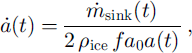
where ρ ice is the ice density.
Knowing the volume fraction θ ice of ice in the layer, the lattice constant k is given by:

where VL(t) is the ice volume per unit cell due to intralayer transport, VL2L(t) is the ice volume per unit cell due to L2L transport, and ρlay is the dry-snow density of the layer. Because the intralayer transport conserves mass, VL(t) is simply:

Combining Equations (5–8), grain growth rate may now be expressed as:

VL2L(t) is obtained by integrating ΔmL2L(t)k2(t) (cf Equation (3)) over time:

Finally, grain-size a(t) is calculated by integrating Equation (9) over time:
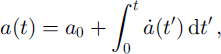
where t’ is an integration variable in both Equations (10) and (11).
Methods
Grain-growth experiments
Seven experiments on kinetic-growth metamorphism which were performed in the cold laboratory at SLF are reported. In six experiments, snow was collected after recent snowfalls and sieved into a well-insulated box with a temperature-controlled heater at the bottom. The characteristics of the experiments are summarized in Table 1. The temperature of the investigated samples was brought to a uniform value of –10°C for experiments 1–6 and to about –4°C in experiment 7. After inducing the temperature gradient, samples were collected and analyzed at chosen time intervals. More experimental details can be found in Reference PielmeierPielmeier (1998), Reference BaunachBaunach (1999) and Reference Fierz and BaunachFierz and Baunach (2000).
Characteristics of seven experiments performed in the cold laboratory

Experimental results are compared with simulations from the modular one-dimensional snow-cover model SNOW-PACK (Reference Lehning, Bartelt, Brown, Russi, Stockli and ZimmerliLehning and others, 1999). The modelled snow layer was made up of five elements, the one in the middle representing the investigated samples. Two kinetic-growth algorithms were used, i.e. an implementation of our model and an implementation of Reference MarboutyMarbouty’s (1980) formulation. To calculate L2L transport (Equation (3)), temperatures at the top and bottom of the elements (nodes) as well as the temperature gradient over the element were used, whereas only element properties entered the evaluation of either intralayer transport (Equation (4)) or Marbouty’s formulation.
In both implementations, grains do not grow before their dendricity dd reaches zero. Dendricity determines to what extent snow may be described as consisting of new snow, fragmented or decomposing particles. Dendricity varies from 1 for new snow to 0 for snow with no recognizable precipitation particle. However, as mentioned in Reference Fierz and BaunachFierz and Baunach (2000), dd is difficult to determine experimentally. Hence, in our simulation runs, dd was adjusted to match the beginning of grain growth as observed by the appearance of faceted grains. A uniform initial grain-size of 0.6 mm was used in SNOWPACK, corresponding to the observed sizes at the beginning of the growth phase and facilitating comparison of the simulations. The errors in measuring grain-size were assumed to be of the order of ±10%, whereas the error in simulation outputs was of the order of ±0.25 to ±0.5 mm. The latter errors were attributed to errors in the simulation of the snow layer’s height, temperature gradient and density (Reference BaunachBaunach, 1999).
Determination of grain-size
Different techniques such as sieving, image processing and visual inspection were used to determine mean grain-sizes
 from disaggregated snow samples taken at given time intervals from the insulated metamorphism box.
The sieving process included the use of a cascade of different-sized sieves with an average mesh opening
 between two sieves i, i + 1 . The weight fraction in each sieve Mi
is measured and the mean grain-size
 obtained from (Reference NiggliNiggli, 1939; Reference Friedman and SandersFriedman and Sanders, 1983):
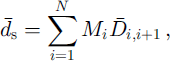
where N is the number of sieves.
Grain-size measurements by image analysis are based on digitized macrophotographs of disaggregated snow samples. Standard image-processing programs (e.g. ImagePro) provide various methods for estimating grain-size. Three of them were considered in this study: average diameter davg , maximum diameter dmax and area equivalent deqar. Average diameter is obtained by averaging the grain’s diameters measured through the centroid at 2° intervals. The maximum diameter is the length of the longest line joining two points of the grain’s contour and passing through the centroid. Area equivalent is the diameter of a circle whose area is equal to the grain’s area, a method often used in former work (Reference MarboutyMarbouty, 1980; Reference Fukuzawa and AkitayaFukuzawa and Akitaya, 1993).
Two additional measures of grain-size were used by Reference Satyawali and AgrawalSatyawali (1994). The first takes width dw and length d1 of a box surrounding the grain, and grain-size df is calculated as:
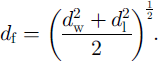
The second takes mutually perpendicular minimum and maximum extensions dmin and dmax to get:

These methods require that any objects on the digitized macrophotographs representing more than one grain be separated into individual objects. Overlapping and touching of grains arose during the preparation of disaggregated samples due to a trade-off between time and ongoing sublimation. For all image-processing methods, the mean grain-size
 was taken over the number of analyzed grains.
Finally, macrophotographs of disaggregated snow samples on a 2 mm grid were presented to six SLF experts for visual characterization. According to Reference ColbeckColbeck and others (1990), they were asked to determine the grain-size dv as a range of the greatest extension of the grains.
Gram-sizes of kinetically grown grains may not be compared directly to sizes deduced from gram-curvature calculations, as was done by Reference Fierz and BaunachFierz and Baunach (2000). Indeed, gram-size derived from curvature does not quite represent the actual observed size of faceted and depth-hoar crystals (Reference Lesaffre, Pougatch and MartinLesaffre and others, 1998).
Results and Discussion
Grain-size
Results from image processing are compared to sieving in Figure 2. Notice the good agreement between sizes obtained by sieving and the average diameters. This agreement is not trivial since two different statistics were used. On the one side, weight fractions were measured, and on the other side a number of single grains were analyzed. Because the form of the grains was highly convoluted, to switch from one statistic to another is not straightforward. This problem is discussed in detail by Reference Sturm and BensonSturm and Benson (1997) and also by Reference HatchHatch (1933). Also notice that the sizes obtained by the equal-area technique he between the maximum and average diameters.
Evolution of gram-size with time, experiment 1: comparison of different methods used to determine gram-size. Solid squares: average diameter. Open squares: maximum diameter. Solid triangles: sieved size. Open circles: area equivalent. Dotted lines are guides to the eye.

Table 2 shows the results obtained with the methods used by Reference Satyawali and AgrawalSatyawali (1994) for three samples from experiment 7 (treated image). They are compared to the average diameter obtained without separating objects into individual grains (raw image). First, note the good agreement between the various methods applied to the treated images. Second, note that the sizes obtained on treated images are smaller, as we would expect. Third, one can see that the ratios of
 (treated) to
 (raw) are similar for all three samples, being smallest for the initial decomposing particles (seeTable 1). Indeed, it is most difficult to separate precipitation particles prior to taking pictures, leading to large overlapping of grains on raw images. This matters less for larger, kinetically grown grains.
Influence of separating objects into individual grains.
 : single-grainferret;
 : single-grain extreme extensions;
: average diameter;
 : equivalent area

Next, consider the comparison of visual characterization with average and maximum diameters obtained from raw images (see Fig. 3). The average range of sizes given by the six experts fits quite well to average and maximum diameter. Since chains of kinetically grown crystals developed during our experiments, some experts may have given the maximum extension of the latter for the upper range value. This explains the large error bars on the expert’s maximum values.
Evolution of grain-size with time, experiment 1: comparison of average and maximum diameter with visual characterization. Solid diamonds: experts’ minimum. Open diamonds: experts’ maximum. Solid squares: average diameter. Open squares: maximum diameter. The error bars indicate the extremes given by any one of the experts, and dotted lines are guides to the eye.

In conclusion, average diameter obtained from image processing, mean size from sieving, and the minimum of the size range given by an expert closely agree for the full range of grain-sizes observed in this study, i.e. 0.5–2.5 mm. Furthermore, at least for kinetically grown grains, a painstaking separation of objects into single grains is not necessary. Therefore, using one of the above methods, there are objectively comparable techniques to determine grain-size. This objectivity is important regarding comparison of snow model outputs with either laboratory results or field observations.
Grain growth
Looking at the results above, the aim for a simple theory of grain growth is to obtain simulated sizes ranging between average and maximum observed grain-size. Modelled grain-sizes (see Equation (11)) that are smaller than the average diameter or larger than the maximum diameter will not correctly represent the experiment. The ultimate goal, however, is to approximate the observed average diameters as closely as possible.
The contributions to grain growth from intralayer jL and L2L transport are shown in Figure 4. Grain-size was simulated for experiment 1, considering either both mechanisms (solid line) or only intralayer transport (dashed line). Note that intralayer flux will lead to saturation as the sources are consumed, but it is predominant as shown also by Reference Sturm and BensonSturm and Benson, (1997). However, saturation is overcome by the smaller but steady L2L transport. Furthermore, in our experiments, no additional changes in density were observed after initial settling. This limiting behaviour is also consistent with a predominance of intralayer transport.
Evolution of grain-size with time, experiment 1: VT = –120Km−1, p = 100 kgm3. Solid line: simulation including both intralayer and L2L contributions, f = 1. Dashed line: simulation including intralayer contribution only, f = 1. Solid squares: average diameter. Open squares: maximum diameter.

Figure 5 shows the influence of the geometric parameter f on simulated grain-size for experiment 1. Setting f to 8 in our model was found to fit best the results for all conditions encountered in our experiments.
Evolution of grain-size with time, experiment 1: VT = –120Km−1, p = 100 kgm3. Solid line: simulation including both intralayer and L2L contributions, f = 8 Dashed line: simulation including both intralayer and L2L contributions, f = 1. Solid squares: average diameter. Open squares: maximum diameter.

However, the model has its limitations. In experiment 6 (Fig. 6), a temperature gradient of –350 K m−1 was established. The simulated grain-size a(t) was close to the maximum diameter, whereas Reference MarboutyMarbouty’s (1980) formulation yielded results closer to the average diameter, at least for this short time period of 3 days. This is a clear indication that the assumption of linear diffusion fails (Fick’s law, Equation (1)) and that it is necessary to limit the influence of large temperature gradients. Indeed, at temperatures below –20°C, even temperature gradients as large as –500 Km−1 do not boost grain growth which is mainly temperature-dependent (Reference Kamata, Sokratov, Sato, Hutter, Wang and BeerKamata and others, 1999).
Evolution of grain-size with time, experiment 6: ∇T = –350 Km−1, p = 110 kg m−3. Solid squares: average diameter. Open squares: maximum diameter. Solid triangles: sieved size. Solid line: simulation including both intralayer and L2L contributions, f = 8 Dashed line: simulation with Reference MarboutyMarbouty’s (1980) formulation.

An overview of all experiments is presented in Figure 7. Experimental growth rates were obtained from linear least-squares fits of the average diameter during the growth phase (see Fig. 4) even though the time dependencies were not linear. Only simulation results obtained with a geometric parameter f = 8 are shown. Despite the outliers for experiments 4 and 6 (ellipses in Fig. 7), the overall agreement between observation and simulation is satisfactory. For large observed growth rates, Reference MarboutyMarbouty’s (1980) formulation usually underestimates growth as expected from the results by Reference Fukuzawa and AkitayaFukuzawa and Akitaya (1993).
Simulated growth rate vs growth rate deduced from average diameter values. Solid triangles: simulations including both intralayer and L2L contributions, f = 8. Crosses: simulations with Marbouty’s formulation. Solid line: average diameter (1:1 line). Dashed line: maximum diameter (linear fit).

In view of the above results, it is interesting to compare in more detail our model with Marbouty’s formulation. Marbouty’s empirical formula for growth rate considers the influence of temperature, density and temperature gradient on kinetic growth rate (Reference MarboutyMarbouty 1980). In our model, temperature effects on growth rate
 are represented by both the exponential temperature dependence of saturation pressure and the term T−3 in Equation (2). Thus these temperature dependencies limit growth at lower temperatures, as does Marbouty’s formulation. Growth rate is reduced at high snow densities also (Equation (9)), as in Marbouty’s formulation. At very low densities, however, growth rate would go to infinity. As densities of <30 kg m−3 are seldom observed in nature, this value is used as a lower cut-off in the model.
Because a linear diffusion theory is used (Fick’s law, Equation (1)), the dependency on temperature gradient is linear too. This contrasts with the non-linearity empirically introduced by Marbouty. This difference becomes significant under extreme conditions, as shown in Figures 6 and 7 for experiment 6 (∇T = –350Km−1). Moreover the diffusion coefficient is assumed to be constant during the experiment, though the development of depth-hoar chains is expected to alter it.
Whereas Marbouty’s growth rate is linear in time, Equation (9) shows that growth rate is not linear in time in our model and depends on the actual grain-size a(t). Hence growth rate decreases with both time and increasing grain-size, a fact which is intuitively correct and has been observed by Reference Sturm and BensonSturm and Benson (1997).
Conclusions
Various methods used to determine grain-sizes both in the laboratory and in the field were compared. Simulation outputs were objectively compared with grain-sizes obtained by these different techniques and by field observations.
A new, physically based model for kinetic grain growth was presented. It takes into account both intralayer and L2L water-vapour transport. Growing sink grains are not taken as spherical but as plate-like. The simplicity of the bcc geometry used as the model’s basis makes it necessary to introduce a geometric parameter f. It is found that for f = 8, the model provides satisfactory results for snow densities of 100–200 kg m–3 and temperature gradients up to –200 K m−1. However the model fails under extreme conditions. Despite its simplicity it performs at least as well as the empirical formulation of Reference MarboutyMarbouty (1980).
The model might be improved by further experiments at other temperatures, as well as by validation with field observations, but some of its limitations will be overcome only by considering non-linearity in both temperature gradient and temperature. Furthermore, more realistic descriptions of an ensemble of interconnected grains (texture) will be needed in future snow-metamorphism models, leaving behind the oversimplified grain-to-grain picture and the bcc texture used here.
Acknowledgements
The authors would like to thank P. Bartelt, G. Camponovo, P. M. B. Fohn, M. Lehning and C. Pielmeier for many fruitful discussions. Special thanks to R. Wetter, C. Simeon and M. Hiller who helped set up the experiment and acquire the necessary data. The authors are especially indebted to C. Coléou, B. Lesaffre and E. Pougatch (Centre d’Etudes de la Neige, Grenoble, France), who gave much advice on successfully processing pictures of disaggregated snow and, in particular, on development of a computer routine to calculate the curvature of snow crystals. The authors appreciate the helpful comments of J. Schweizer on an earlier version of the paper, as well as the insightful reviews of E. E. Adams and L. McKittrick.



