1 Introduction
The basic nature of the global dynamics of gravitational (i.e. spatially developing) liquid sheet flows, in the presence of surface tension effects, depends crucially on the inlet Weber number,
 $We=\unicode[STIX]{x1D70C}_{l}U_{in}^{2}H_{in}/2\unicode[STIX]{x1D70E}$
, where
 $\unicode[STIX]{x1D70C}_{l}$
is the liquid density,
 $U_{in}$
the inlet liquid velocity,
 $H_{in}$
the initial thickness of the sheet,
 $\unicode[STIX]{x1D70E}$
the air–liquid surface tension. When
 $We>1$
, the local Weber number,
 $We_{l}=U^{2}/c^{2}$
, with
 $U$
and
 $c=\sqrt{2\unicode[STIX]{x1D70E}/(\unicode[STIX]{x1D70C}_{l}H)}$
being the local flow and capillary waves velocity (de Luca & Costa Reference de Luca and Costa1997b
), respectively, is also greater than unity at each streamwise location, so that the flow can be defined as supercritical everywhere. When
 $We<1$
, an initial region exists where the sheet flow is subcritical, up to the critical location, downstream of which the flow becomes supercritical. In a previous paper about the unsteady dynamics of water bells, Brunet, Clanet & Limat (Reference Brunet, Clanet and Limat2004), resorting to an analogy between sound waves and capillary waves, termed the line separating the two regions transonic. From a theoretical viewpoint, the problem under study is not straightforward, because it is known (Finnicum, Weinstein & Rushak Reference Finnicum, Weinstein and Rushak1993; Weinstein et al.
Reference Weinstein, Clarke, Moon and Simister1997; Ramos Reference Ramos2001, Reference Ramos2003) that the equation governing the evolution of small disturbances exhibits a singularity just at the critical station and the solution to the problem has not yet been found. All these authors evidence and analyse the nature of the singularity, but no one has definitely solved the time-dependent equations governing the behaviour of the subcritical nappe. Thus, the present work aims at facing the problem to make up for this lack of information.
Although physically the singularity is due to surface tension effects, and therefore it can occur in various situations involving different models of external ambient pressure interacting with the liquid sheet, in this paper we will refer to the so-called nappe oscillation configuration. It is well known that a thin water sheet (curtain or nappe), flowing freely from a top opening, gives rise to low-frequency periodic oscillations when interacting with an air enclosure which acts as a resonator. Such a behaviour, commonly referred to as the nappe oscillation phenomenon (Schwartz Reference Schwartz1964), arises from a mutually induced mechanism among the oscillations of the curtain and the pressure fluctuations in the air enclosure adjacent to one side of the sheet, with the other one being in contact with an unperturbed ambient (Naudascher & Rockwell Reference Naudascher and Rockwell1994). The flow of waterfalls, naturally outpoured or generated by the overflow of water over long crests of dams or weirs, represents a typical example of such a configuration. The noise produced by the oscillation of the waterfall can be radiated far away from the source and may cause problems such as vibrations in doors or windowpanes in buildings nearby, and even structural damages to the dam itself (Crookston & Tullis Reference Crookston and Tullis2013). In this paper it will be shown that, around the critical regime, the theory predicts a sharp increase in nappe oscillation frequency as the flow Weber number is gradually reduced, from supercritical to subcritical values.
Theoretically, the physical problem involves a spatially developing fluid flow system which is able to sustain a variety of wave patterns. Although the spatio-temporal evolution of planar free-falling liquid sheet flows has been widely discussed, mainly in the context of linear stability analysis (Lin, Lian & Creighton Reference Lin, Lian and Creighton1990; de Luca & Costa Reference de Luca and Costa1997a ; de Luca Reference de Luca1999; Barlow, Helenbrook & Lin Reference Barlow, Helenbrook and Lin2011), little attention has been paid to modelling the global coupling between advection and reaction effects (where the term global refers to the system as a whole) when the curtain interacts with a closed air chamber. Binnie (Reference Binnie1974) carried out the first relevant study addressing the nappe oscillation phenomenon from both theoretical and experimental points of view. In particular, he formulated a linearized physical model governing the spatio-temporal evolution of disturbances where surface tension effects were neglected. The flow patterns emerging in his experiments, limited to supercritical regimes, were related to the single modes of the eigenvalues spectrum. Binnie (Reference Binnie1974) suggested that the actual frequency selection mechanism could depend on interfacial viscous shear, due to the ambient air and ignored in the theory. Among more recent experimental contributions noticeable are the works of Sato et al. (Reference Sato, Miura, Nagamine, Morii and Ohkubo2007), and Mori et al. (Reference Mori, Nagamine, Ito and Sato2012), who found a strong correlation between the oscillation frequency of the water sheet and the pressure fluctuation in the adjacent air chamber. They also carried out a theoretical analysis to examine the modal stability of the sheet vibration by means of a complex eigenvalue problem, and compared the less stable mode frequency with the characteristic frequency of a one-degree-of-freedom spring–mass system, with the air into the enclosure being considered as a spring and the water sheet being modelled as a mass. However, the characteristic frequency of the most unstable mode is from 10- to 20 times larger than the frequency experimentally observed in visualizing the nappe oscillation in supercritical conditions. Even the shape of the associate eigenfunction is completely different than that monitored in experiments.
Le Grand et al. (Reference Le Grand, Brunet, Lebon and Limat2006) reported theoretical as well as experimental findings on the characteristics of the global dynamics of liquid sheets, but their work is concerned with a different context, i.e. the case of symmetrical semi-infinite boundary air environments.
Within the framework of the linear non-modal stability theory Schmid & Henningson (Reference Schmid and Henningson2002) found time-periodic oscillations in the optimal amplification of the disturbances energy, and correlated the period of such oscillations to the quasi-constant spacing among the imaginary parts of eigenvalues. They concluded that the phenomenon under study is governed not by a single mode, but by the (linear) interaction of many modes. Such a global feature of the spectrum, obtained neglecting the surface tension, closely agrees with the low-frequency oscillations typically observed in real systems, as confirmed also by Coppola & de Luca (Reference Coppola and de Luca2006) who considered a general toy model.
The global dynamics of nappe oscillation has been recently revisited by De Rosa, Girfoglio & de Luca (Reference De Rosa, Girfoglio and de Luca2014), who extended the analysis of Schmid & Henningson (Reference Schmid and Henningson2002), and found a strong analogy to the edge-tones problem, i.e. acoustic tones produced when a jet of air strikes a wedge-shaped edge; a simple relationship determining the dimensionless resonance frequencies was also reported. Following De Rosa et al. (Reference De Rosa, Girfoglio and de Luca2014), in the present paper the flow is assumed inviscid and the problem is arranged in a one-dimensional formulation along the streamwise direction. The interaction with the external environment refers to an air enclosure located on one side of the sheet. Physical insights on sheet centreline sinuous modes will show that the nappe dynamics features the propagation of two wave fronts both directed downstream or one downstream and the other one upstream, depending on whether the flow is supercritical or subcritical, respectively. In every situation the inlet section is considered as a perfectly reflecting boundary. As regards an additional boundary condition, in the former regime it prescribes a null centreline slope at the inlet; in the latter it is imposed just at the singularity station, by enforcing the boundedness requirement of the centreline slope there. An additional analytical investigation on the nature of the singularity, based on the Frobenius theory, predicts that the flow is unconditionally stable for any
 $We<1$
and that the temporal growth rate of disturbances is bounded.
The findings of the spectral analysis confirm the theoretical predictions anticipated above. They closely agree with numerical simulations of the partial differential equation governing the global evolution of the disturbances in the space–time domain, starting from an initial Gaussian-like shape. Data also agree quantitatively with previous experimental findings of the literature at relatively high Weber numbers (supercritical regime).
The paper is organized as follows: the physical model is developed in § 2, with the overall insights on the nappe dynamics being reported in § 3. The linear stability analysis, including the description of the procedure employed to remove the singularity of the operator, is illustrated in § 4. The overall results are presented in § 5 and major conclusions are drawn up in § 6.
2 Physical modelling
To derive a physical model of the unsteady evolution of an inviscid gravitational liquid sheet, the assumptions of thin curtain and plug flow are adopted (Mehring & Sirignano Reference Mehring and Sirignano1999; Coppola, De Rosa & de Luca Reference Coppola, De Rosa and de Luca2013; De Rosa et al. Reference De Rosa, Girfoglio and de Luca2014). It has to be stressed in particular that, contrary to the recent paper of De Rosa et al. (Reference De Rosa, Girfoglio and de Luca2014), the surface tension effect is fully included since, as will be discussed later on, the presence of the singularity at the critical line depends crucially on the surface tension.
Although in principle singularities arise also in aerated or open configurations (Finnicum et al. Reference Finnicum, Weinstein and Rushak1993; Weinstein et al. Reference Weinstein, Clarke, Moon and Simister1997; Ramos Reference Ramos2001, Reference Ramos2003; Brunet et al. Reference Brunet, Clanet and Limat2004), here we consider the boundary pressure field within a two-dimensional air enclosure delimited by the sheet itself, rigid walls and a lower basin; namely, we will address the unsteady behaviour of the configuration generally referred to as nappe oscillation. Splashing effects are neglected. Furthermore, the investigation will be restricted to the occurrence of one-dimensional surface wave patterns. One can expect that oblique waves (i.e. developing along the spanwise direction) occur when extending the study to three-dimensional configurations, as already found experimentally by Le Grand et al. (Reference Le Grand, Brunet, Lebon and Limat2006) in the case of symmetrical semi-infinite boundary air environments.
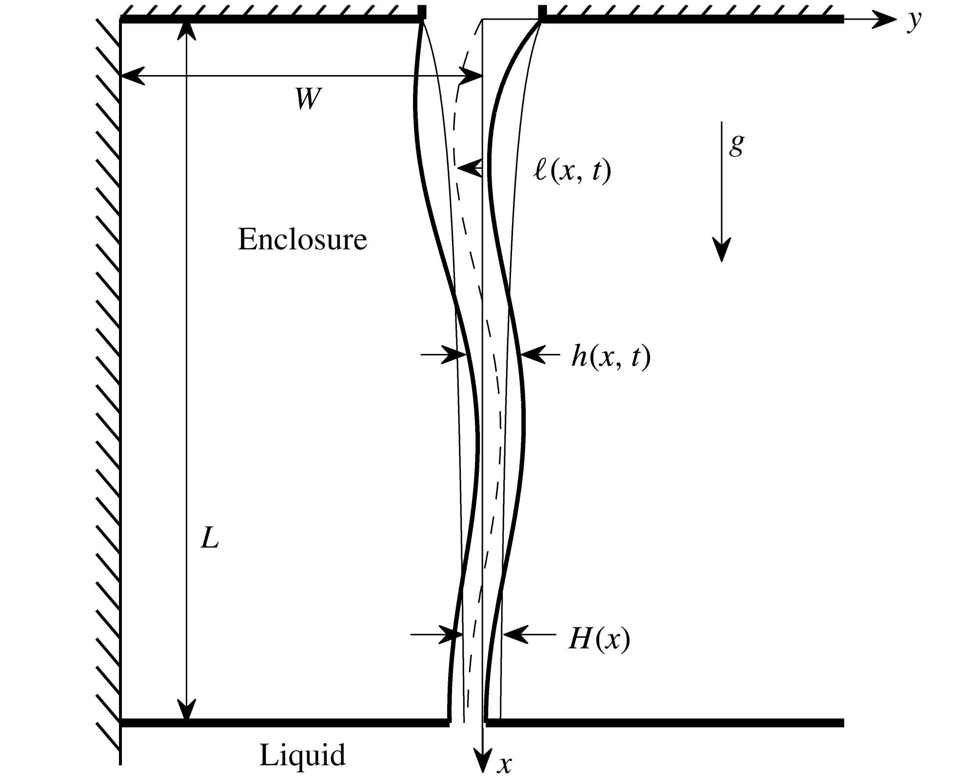
Figure 1 shows the schematic of the geometrical configuration under consideration. In the unperturbed condition the liquid flows along the vertical
 $x$
-direction with a steady velocity and two symmetrical free interfaces. The definitions of the unsteady centreline location
 $\ell$
and thickness
 $h$
of the sheet are given, in terms of the interface positions
 $y^{\pm }$
, as follows
 $$\begin{eqnarray}\displaystyle & \displaystyle \ell ^{\star }(x^{\star },t^{\star })=\frac{y^{\star +}(x^{\star },t^{\star })+y^{\star -}(x^{\star },t^{\star })}{2} & \displaystyle\end{eqnarray}$$
 $$\begin{eqnarray}\displaystyle & \displaystyle h^{\star }(x^{\star },t^{\star })=y^{\star +}(x^{\star },t^{\star })-y^{\star -}(x^{\star },t^{\star }), & \displaystyle\end{eqnarray}$$
where superscripts
 $\pm$
refer to right and left interfaces, respectively, and
 $t^{\ast }$
is the time. Here as elsewhere the star denotes dimensional quantities. Note that the inlet velocity and sheet thickness of the basic flow employed in the Introduction to define the Weber number were denoted without a star apex, for the sake of simplicity; the star is omitted similarly in figure 1. Furthermore, the general definition
 $\unicode[STIX]{x1D711}^{\star \pm }(x^{\star },t^{\star })=\unicode[STIX]{x1D711}^{\star }(x^{\star },y^{\star \pm },t^{\star })$
will be adopted in the following,
 $\unicode[STIX]{x1D711}$
being any of the flow variables
 $u$
,
 $v$
or
 $p$
(where
 $u$
and
 $v$
are the streamwise and lateral liquid velocity components, respectively, and
 $p$
is liquid pressure).
Sketch of the model configuration.

2.1 Governing equations
The starting mathematical framework is given by the two-dimensional Euler equations in which gravity is retained, closed by the kinematic and dynamic conditions imposed at the free interfaces.
The assumption of a thin sheet with respect to the wavelength of a disturbance allows one to consider local plug-type velocity profiles for
 $u$
and
 $v$
across the nappe thickness. To derive the governing equations the following procedure can be adopted: the mass and
 $x$
-momentum balances are formulated over a generic slice of the curtain of length
 $\text{d}x$
; the
 $y$
-momentum equation is integrated along the lateral coordinate
 $y$
; the unsteady quantities are considered as the sum of a steady contribution and a perturbation (or fluctuation)
 $$\begin{eqnarray}\displaystyle & \displaystyle u^{\ast }=U^{\ast }+u^{\prime \ast } & \displaystyle\end{eqnarray}$$
 $$\begin{eqnarray}\displaystyle & \displaystyle v^{\ast }=V^{\ast }+v^{\prime \ast } & \displaystyle\end{eqnarray}$$
 $$\begin{eqnarray}\displaystyle & \displaystyle p^{\ast }=P^{\ast }+p^{\prime \ast } & \displaystyle\end{eqnarray}$$
 $$\begin{eqnarray}\displaystyle & \displaystyle h^{\ast }=H^{\ast }+h^{\prime \ast } & \displaystyle\end{eqnarray}$$
 $$\begin{eqnarray}\displaystyle & \displaystyle y^{\ast \pm }=Y^{\ast \pm }+y^{\prime \ast \pm }, & \displaystyle\end{eqnarray}$$
where capital letters (here as elsewhere) denote basic (steady) quantities and prime the corresponding perturbations. Under the assumption of small perturbations, and
 $V^{\ast }=0$
, the linearized forms of continuity,
 $x$
-momentum and
 $y$
-momentum equations are written, respectively:
 $$\begin{eqnarray}\displaystyle & \displaystyle {\displaystyle \frac{\unicode[STIX]{x2202}h^{\prime \star }}{\unicode[STIX]{x2202}t^{\star }}}+{\displaystyle \frac{\unicode[STIX]{x2202}}{\unicode[STIX]{x2202}x^{\star }}}\left(U^{\star }h^{\prime \star }+H^{\star }u^{\prime \star }\right)=0 & \displaystyle\end{eqnarray}$$
 $$\begin{eqnarray}\displaystyle & \displaystyle {\displaystyle \frac{\unicode[STIX]{x2202}u^{\prime \star }}{\unicode[STIX]{x2202}t^{\star }}}+{\displaystyle \frac{\unicode[STIX]{x2202}}{\unicode[STIX]{x2202}x^{\star }}}\left(U^{\star }u^{\prime \star }\right)=-{\displaystyle \frac{1}{\unicode[STIX]{x1D70C}_{l}}}{\displaystyle \frac{\unicode[STIX]{x2202}p^{\prime \star }}{\unicode[STIX]{x2202}x^{\star }}} & \displaystyle\end{eqnarray}$$
 $$\begin{eqnarray}\displaystyle & \displaystyle {\displaystyle \frac{\unicode[STIX]{x2202}v^{\prime \star }}{\unicode[STIX]{x2202}t^{\star }}}+U^{\star }{\displaystyle \frac{\unicode[STIX]{x2202}v^{\prime \star }}{\unicode[STIX]{x2202}x^{\star }}}=-{\displaystyle \frac{1}{\unicode[STIX]{x1D70C}_{l}H^{\star }}}(p^{\prime \star +}-p^{\prime \star -}), & \displaystyle\end{eqnarray}$$
where
 $\unicode[STIX]{x1D70C}_{l}$
is the liquid density.
The interface kinematic and pressure jump boundary conditions are, respectively:
 $$\begin{eqnarray}\displaystyle & \displaystyle v^{\star \pm }={\displaystyle \frac{\unicode[STIX]{x2202}y^{\star \pm }}{\unicode[STIX]{x2202}t^{\star }}}+u^{\star \pm }{\displaystyle \frac{\unicode[STIX]{x2202}y^{\star \pm }}{\unicode[STIX]{x2202}x^{\star }}} & \displaystyle\end{eqnarray}$$
 $$\begin{eqnarray}\displaystyle & \displaystyle p^{\star \pm }=p_{a}^{\star \pm }\mp \unicode[STIX]{x1D70E}{\displaystyle \frac{\unicode[STIX]{x2202}^{2}y^{\star \pm }}{\unicode[STIX]{x2202}x^{\star 2}}}\left[1+\left({\displaystyle \frac{\unicode[STIX]{x2202}y^{\star \pm }}{\unicode[STIX]{x2202}x^{\star }}}\right)^{2}\right]^{-3/2}, & \displaystyle\end{eqnarray}$$
where
 $p_{a}^{\star \pm }(x^{\star },t^{\star })$
is the local value of the external ambient pressure and
 $\unicode[STIX]{x1D70E}$
is the surface tension coefficient.
The difference between the fluctuating boundary pressures of (2.10) can be expressed in terms of perturbations of ambient pressure and interface locations by linearizing in perturbation quantities the dynamic boundary condition (2.12):
 $$\begin{eqnarray}p^{\prime \star \pm }=p_{a}^{\prime \star \pm }\mp \unicode[STIX]{x1D70E}\left[1+\left({\displaystyle \frac{\text{d}Y^{\star \pm }}{\text{d}x^{\star }}}\right)^{2}\right]^{-3/2}\cdot \left\{{\displaystyle \frac{\unicode[STIX]{x2202}^{2}y^{\prime \star \pm }}{\unicode[STIX]{x2202}x^{\star 2}}}-3{\displaystyle \frac{\displaystyle \frac{\text{d}^{2}Y^{\star \pm }}{\text{d}x^{\star 2}}\frac{\text{d}Y^{\star \pm }}{\text{d}x^{\star }}\frac{\unicode[STIX]{x2202}y^{\prime \star \pm }}{\unicode[STIX]{x2202}x^{\star }}}{1+\displaystyle \left(\frac{\text{d}Y^{\star \pm }}{\text{d}x^{\star }}\right)^{2}}}\right\}.\end{eqnarray}$$
The result is then recast in the form:
 $$\begin{eqnarray}p^{\prime \star +}-p^{\prime \star -}=\widetilde{p}_{a}^{\prime \star }-2\unicode[STIX]{x1D70E}{\displaystyle \frac{\unicode[STIX]{x2202}}{\unicode[STIX]{x2202}x^{\star }}}\left[F^{\star }{\displaystyle \frac{\unicode[STIX]{x2202}\ell ^{\prime \star }}{\unicode[STIX]{x2202}x^{\star }}}\right],\end{eqnarray}$$
with
 $F^{\star }=[1+(\text{d}H^{\star }/\text{d}x^{\star })^{2}/4]^{-3/2}$
, and
 $\widetilde{p}_{a}^{\star }=p_{a}^{\star +}-p_{a}^{\star -}$
. Note also that
 $|Y^{\ast \pm }|=H^{\ast }/2$
.
Equation (2.10) has to be coupled with the linearized kinematic boundary condition, which can be properly expressed in terms of the centreline deflection only:
 $$\begin{eqnarray}v^{\prime \star }={\displaystyle \frac{\unicode[STIX]{x2202}\ell ^{\prime \star }}{\unicode[STIX]{x2202}t^{\star }}}+U^{\star }{\displaystyle \frac{\unicode[STIX]{x2202}\ell ^{\prime \star }}{\unicode[STIX]{x2202}x^{\star }}}.\end{eqnarray}$$
Equations (2.10) and (2.15) constitute a closed system for the unknown lateral velocity and centreline perturbations, representing the so called antisymmetric sinuous solution to the unsteady perturbed field.
It is easily observed that (2.8) and (2.9) represent, on the other hand, the symmetric, or varicose, or even squeezing solution for the perturbed longitudinal velocity and sheet thickness. In fact, the liquid pressure (which is constant in this symmetric case, i.e.
 $p^{\prime \star }=p^{\prime \star +}=p^{\prime \star -}$
) can be eliminated by taking the half-sum of the right-hand side of (2.13) so as to obtain
 $$\begin{eqnarray}p^{\prime \star }=\overline{p}_{a}^{\prime \star }-{\displaystyle \frac{\unicode[STIX]{x1D70E}}{2}}{\displaystyle \frac{\unicode[STIX]{x2202}}{\unicode[STIX]{x2202}x^{\star }}}\left[F^{\star }{\displaystyle \frac{\unicode[STIX]{x2202}h^{\prime \star }}{\unicode[STIX]{x2202}x^{\star }}}\right],\end{eqnarray}$$
where
 $$\begin{eqnarray}\displaystyle \overline{p}_{a}^{\star }=\frac{p_{a}^{\star +}+p_{a}^{\star -}}{2}. & & \displaystyle\end{eqnarray}$$
To close the two systems of coupled equations (2.8)–(2.9) and (2.10)–(2.15), expressions for the ambient gas pressure terms
 $\overline{p}_{a}^{\prime \star }$
and
 $\widetilde{p}_{a}^{\prime \star }$
as functions of the perturbations of the sheet are required.
The infinitesimal variation of the enclosure volume, resulting from the sheet fluctuation, is given by
 $$\begin{eqnarray}\displaystyle {\mathcal{V}}_{a}^{\prime \star }=\int _{0}^{L^{\star }}\ell ^{\prime \star }(x^{\star })\,\text{d}x^{\star }-{\displaystyle \frac{1}{2}}\int _{0}^{L^{\star }}h^{\prime \star }(x^{\star })\,\text{d}x^{\star }. & & \displaystyle\end{eqnarray}$$
If we hypothesize that the air within the enclosure encompasses compression/expansion isentropic thermodynamic transformations, we are able to give explicit expressions for the external pressure terms of (2.14) and (2.16), for the two different oscillating modes of the sheet, respectively, as follows:
 $$\begin{eqnarray}\displaystyle & \displaystyle \widetilde{p}_{a}^{\prime \star }=\unicode[STIX]{x1D6FE}{\displaystyle \frac{P_{a}^{\star }}{{\mathcal{V}}_{a}^{\star }}}\int _{0}^{L^{\star }}\ell ^{\prime \star }(x^{\star })\,\text{d}x^{\star } & \displaystyle\end{eqnarray}$$
 $$\begin{eqnarray}\displaystyle & \displaystyle \overline{p}_{a}^{\prime \star }={\displaystyle \frac{\unicode[STIX]{x1D6FE}}{4}}{\displaystyle \frac{P_{a}^{\star }}{{\mathcal{V}}_{a}^{\star }}}\int _{0}^{L^{\star }}h^{\prime \star }(x^{\star })\,\text{d}x^{\star }, & \displaystyle\end{eqnarray}$$
where
 $\unicode[STIX]{x1D6FE}$
is the specific heat ratio,
 $P_{a}^{\star }$
is the unperturbed gas pressure into the enclosure and
 ${\mathcal{V}}_{a}^{\star }=L^{\star }W^{\star }-\int _{0}^{L^{\star }}H^{\star }(x^{\star })\,\text{d}x^{\star }/2$
is the corresponding volume in the configuration shown in figure 1.
Substituting the above relationships of the pressure difference and of the average pressure into the streamwise and lateral momentum equations (2.9) and (2.10), respectively, eventually yields:
 $$\begin{eqnarray}\displaystyle & \displaystyle {\displaystyle \frac{\unicode[STIX]{x2202}u^{\prime \star }}{\unicode[STIX]{x2202}t^{\star }}}+{\displaystyle \frac{\unicode[STIX]{x2202}}{\unicode[STIX]{x2202}x^{\star }}}\left(U^{\star }u^{\prime \star }\right)={\displaystyle \frac{\unicode[STIX]{x1D70E}}{2\unicode[STIX]{x1D70C}_{l}}}{\displaystyle \frac{\unicode[STIX]{x2202}^{2}}{\unicode[STIX]{x2202}x^{\star 2}}}\left[F^{\star }{\displaystyle \frac{\unicode[STIX]{x2202}h^{\prime \star }}{\unicode[STIX]{x2202}x^{\star }}}\right] & \displaystyle\end{eqnarray}$$
 $$\begin{eqnarray}\displaystyle & \displaystyle {\displaystyle \frac{\unicode[STIX]{x2202}v^{\prime \star }}{\unicode[STIX]{x2202}t^{\star }}}+U^{\star }{\displaystyle \frac{\unicode[STIX]{x2202}v^{\prime \star }}{\unicode[STIX]{x2202}x^{\star }}}={\displaystyle \frac{2\unicode[STIX]{x1D70E}}{\unicode[STIX]{x1D70C}_{l}H^{\star }}}{\displaystyle \frac{\unicode[STIX]{x2202}}{\unicode[STIX]{x2202}x^{\star }}}\left[F^{\star }{\displaystyle \frac{\unicode[STIX]{x2202}\ell ^{\prime \star }}{\unicode[STIX]{x2202}x^{\star }}}\right]-{\displaystyle \frac{\unicode[STIX]{x1D6FE}}{\unicode[STIX]{x1D70C}_{l}H^{\star }}}{\displaystyle \frac{P_{a}^{\star }}{{\mathcal{V}}_{a}^{\star }}}\int _{0}^{L^{\star }}\ell ^{\prime \star }(x^{\star })\,\text{d}x^{\star }. & \displaystyle\end{eqnarray}$$
It is worth noting that in deriving (2.21) it is implicitly assumed that the pressure fluctuation inside the air enclosure does not vary in space, according to the model of lumped reaction of the cushion, which is the equivalent of neglecting acoustic modes propagating in the air enclosure. The cushion lumped model is valid if the ratio of the traversing time,
 $t_{a}^{\star }$
, of an acoustic perturbation over a typical dimension of enclosure (say
 $W^{\star }$
), to the oscillation period
 $T^{\star }$
, is sufficiently small. As will be seen later in discussing experimental comparisons, for typical experimental arrangements this assumption is valid up to frequencies of the order of 100 Hz. The set of two systems of coupled equations (2.8)–(2.21) and (2.15)–(2.22), can be also arrived at by using the theory and the methods of perturbations (De Rosa Reference De Rosa2013).
2.2 Non-dimensional equations and slender sheet approximation
The governing equations can be conveniently made dimensionless by employing the reference quantities
 $$\begin{eqnarray}\displaystyle L_{r}^{\star }=L^{\star },\quad \ell _{r}^{\star }=H_{in}^{\star }, & & \displaystyle\end{eqnarray}$$
 $$\begin{eqnarray}\displaystyle u_{r}^{\star }=U_{in}^{\star },\quad v_{r}^{\star }=\unicode[STIX]{x1D700}U_{in}^{\star }, & & \displaystyle\end{eqnarray}$$
 $$\begin{eqnarray}\displaystyle t_{r}^{\star }=L^{\star }/U_{in}^{\star },\quad p_{r}^{\star }=\unicode[STIX]{x1D70C}_{l}U_{in}^{\star ^{2}}, & & \displaystyle\end{eqnarray}$$
with
 $\unicode[STIX]{x1D700}=\ell _{r}^{\star }/L_{r}^{\star }$
denoting the slenderness parameter (tiny according to the assumptions made in deriving the model). The non-dimensional form has the following results
 $$\begin{eqnarray}\displaystyle & \displaystyle {\displaystyle \frac{\unicode[STIX]{x2202}\ell }{\unicode[STIX]{x2202}t}}+U{\displaystyle \frac{\unicode[STIX]{x2202}\ell }{\unicode[STIX]{x2202}x}}=v & \displaystyle\end{eqnarray}$$
 $$\begin{eqnarray}\displaystyle & \displaystyle {\displaystyle \frac{\unicode[STIX]{x2202}v}{\unicode[STIX]{x2202}t}}+U{\displaystyle \frac{\unicode[STIX]{x2202}v}{\unicode[STIX]{x2202}x}}={\displaystyle \frac{1}{WeH}}{\displaystyle \frac{\unicode[STIX]{x2202}}{\unicode[STIX]{x2202}x}}\left[F{\displaystyle \frac{\unicode[STIX]{x2202}\ell }{\unicode[STIX]{x2202}x}}\right]-{\displaystyle \frac{\unicode[STIX]{x1D6FE}}{H}}{\displaystyle \frac{P_{a}}{\unicode[STIX]{x1D700}\displaystyle \left(\frac{W^{\star }}{L^{\star }}-\frac{\unicode[STIX]{x1D700}}{2}\int _{0}^{1}H\,\text{d}x\right)}}\int _{0}^{1}\ell (x)\,\text{d}x & \displaystyle\end{eqnarray}$$
 $$\begin{eqnarray}\displaystyle & \displaystyle {\displaystyle \frac{\unicode[STIX]{x2202}h}{\unicode[STIX]{x2202}t}}+{\displaystyle \frac{\unicode[STIX]{x2202}}{\unicode[STIX]{x2202}x}}(Uh+Hu)=0 & \displaystyle\end{eqnarray}$$
 $$\begin{eqnarray}\displaystyle & \displaystyle {\displaystyle \frac{\unicode[STIX]{x2202}u}{\unicode[STIX]{x2202}t}}+{\displaystyle \frac{\unicode[STIX]{x2202}}{\unicode[STIX]{x2202}x}}(Uu)={\displaystyle \frac{\unicode[STIX]{x1D700}^{2}}{4We}}{\displaystyle \frac{\unicode[STIX]{x2202}^{2}}{\unicode[STIX]{x2202}x^{2}}}\left[F{\displaystyle \frac{\unicode[STIX]{x2202}h}{\unicode[STIX]{x2202}x}}\right], & \displaystyle\end{eqnarray}$$
where
 $$\begin{eqnarray}\displaystyle We=\unicode[STIX]{x1D70C}_{l}U_{in}^{\star ^{2}}H_{in}^{\star }/2\unicode[STIX]{x1D70E} & & \displaystyle\end{eqnarray}$$
is the Weber number, already defined in the Introduction, with the exception of the use of the star apex, and
 $F=[1+\unicode[STIX]{x1D700}^{2}/4(\text{d}H/\text{d}x)^{2}]^{-3/2}$
. Note that (2.26)–(2.27) describe the sinuous modes, whilst (2.28)–(2.29) describe the varicose ones.
As extensively discussed in Coppola et al. (Reference Coppola, De Rosa and de Luca2013), in the absence of viscosity, an analytical solution for sheet thickness and streamwise liquid velocity of the steady (base) flow can be obtained by performing a parameter-type expansion in the small ratio
 $\unicode[STIX]{x1D700}^{2}$
of the unperturbed governing equations. At the zeroth-order expansion, the following non-dimensional Torricelli’s free-fall solution for the base flow results:
 $$\begin{eqnarray}UH=1\quad \text{and}\quad U=\sqrt{1+\frac{2}{Fr}x},\end{eqnarray}$$
where
 $$\begin{eqnarray}\displaystyle Fr=U_{in}^{\star ^{2}}/gL^{\star } & & \displaystyle\end{eqnarray}$$
denotes the Froude number.
Accordingly, the corresponding lowest-order expansion to (2.26)–(2.29) leads to the slender sheet approximation: for the sinuous mode
 $$\begin{eqnarray}\displaystyle & \displaystyle {\displaystyle \frac{\unicode[STIX]{x2202}\ell }{\unicode[STIX]{x2202}t}}+U{\displaystyle \frac{\unicode[STIX]{x2202}\ell }{\unicode[STIX]{x2202}x}}=v & \displaystyle\end{eqnarray}$$
 $$\begin{eqnarray}\displaystyle & \displaystyle {\displaystyle \frac{\unicode[STIX]{x2202}v}{\unicode[STIX]{x2202}t}}+U{\displaystyle \frac{\unicode[STIX]{x2202}v}{\unicode[STIX]{x2202}x}}={\displaystyle \frac{1}{WeH}}{\displaystyle \frac{\unicode[STIX]{x2202}^{2}\ell }{\unicode[STIX]{x2202}x^{2}}}-{\displaystyle \frac{{\mathcal{K}}}{H}}\bar{\ell } & \displaystyle\end{eqnarray}$$
and for the varicose mode
 $$\begin{eqnarray}\displaystyle & \displaystyle {\displaystyle \frac{\unicode[STIX]{x2202}h}{\unicode[STIX]{x2202}t}}+{\displaystyle \frac{\unicode[STIX]{x2202}}{\unicode[STIX]{x2202}x}}(Uh+Hu)=0 & \displaystyle\end{eqnarray}$$
 $$\begin{eqnarray}\displaystyle & \displaystyle {\displaystyle \frac{\unicode[STIX]{x2202}u}{\unicode[STIX]{x2202}t}}+{\displaystyle \frac{\unicode[STIX]{x2202}}{\unicode[STIX]{x2202}x}}(Uu)=0, & \displaystyle\end{eqnarray}$$
with
 $$\begin{eqnarray}\displaystyle {\mathcal{K}}=\unicode[STIX]{x1D6FE}\frac{P_{a}}{\unicode[STIX]{x1D700}}\frac{L^{\star }}{W^{\star }} & & \displaystyle\end{eqnarray}$$
and
 $$\begin{eqnarray}\displaystyle \bar{\ell }=\int _{0}^{1}\ell \,\text{d}x & & \displaystyle\end{eqnarray}$$
denoting the average sinuous deflection of the sheet.
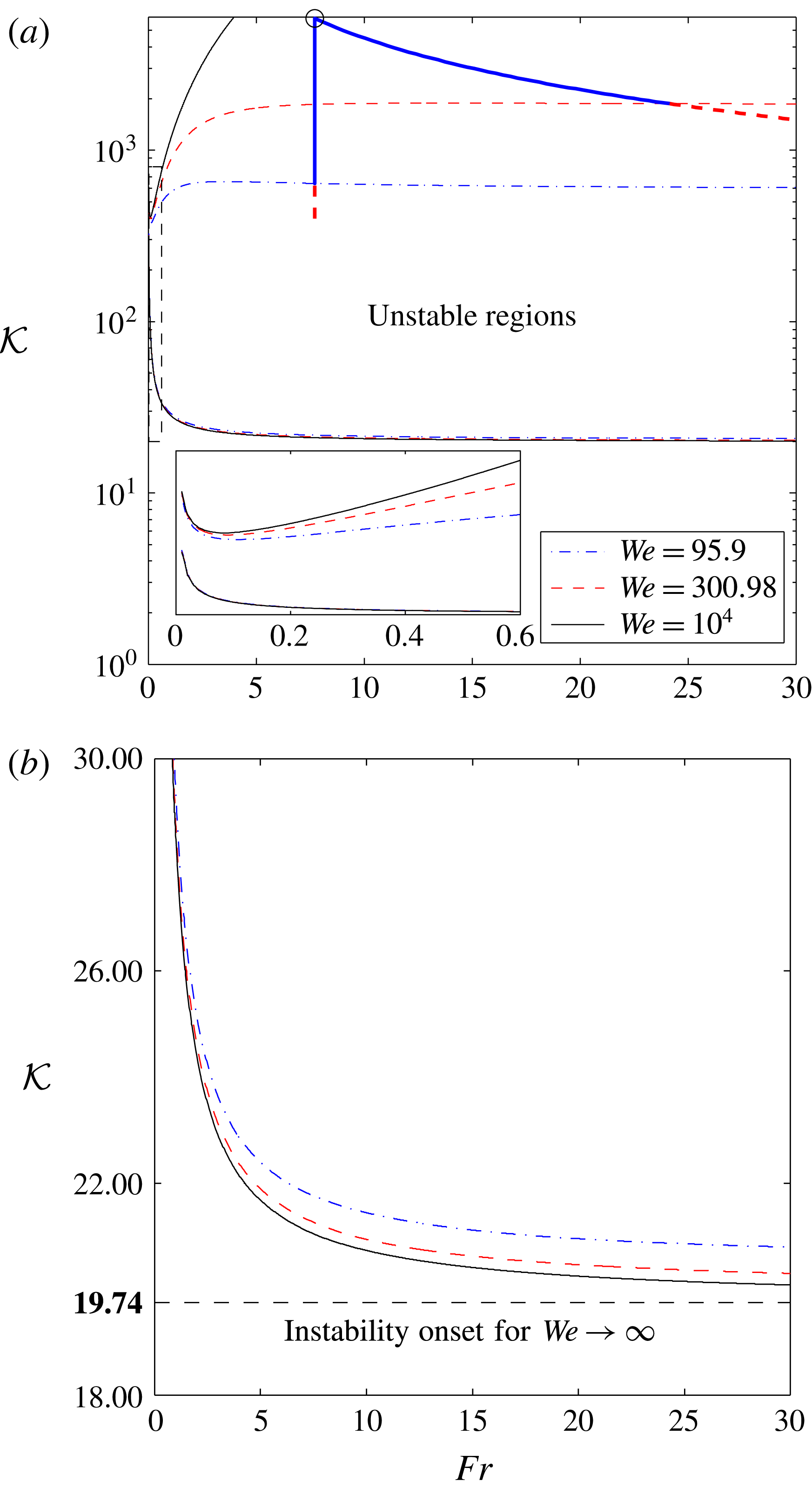
To sum up, three independent dimensionless parameters for the problem under study are considered: the Weber number
 $We$
, the Froude number
 $Fr$
and the equivalent air stiffness
 ${\mathcal{K}}$
. Note explicitly that in the present analysis the air stiffness includes simultaneously the effects of the undisturbed pressure within the enclosure, of the enclosure width and of the slenderness ratio
 $\unicode[STIX]{x1D700}=H_{in}^{\star }/L^{\star }$
, which in principle have to be taken into account separately. More importantly, one should note that, for practical physical cases of water sheet surrounded by air,
 $\unicode[STIX]{x1D70C}_{l}$
,
 $\unicode[STIX]{x1D70E}$
,
 $\unicode[STIX]{x1D6FE}$
and
 $P_{a}^{\star }$
have to be considered as fixed quantities, and it is easy to verify that given values of the dimensionless quantities
 $We$
,
 $Fr$
,
 ${\mathcal{K}}$
and
 $\unicode[STIX]{x1D700}$
determine a unique set of values
 $U_{in}^{\star }$
,
 $H_{in}^{\star }$
,
 $L^{\star }$
and
 $W^{\star }$
, and vice versa.
Note also that (2.35)–(2.36) governing the evolution of the varicose modes are not able to sustain any oscillating wave pattern in the configuration here adopted, reducing to simple advection equations. Therefore, the study will be focused hereinafter on the sinuous disturbances only, equations (2.33)–(2.34). Particular attention has to be paid to enforce the boundary conditions depending on whether the inlet Weber number is supercritical or subcritical. In fact, in the first case two boundary conditions are prescribed at the inlet location,
 $x=0$
, namely
 $\ell (0)=0$
and
 $\unicode[STIX]{x2202}\ell /\unicode[STIX]{x2202}x(0)=0$
(which in turn means
 $v(0)=0$
), whilst in the latter case the condition,
 $\ell (0)=0$
, is retained at the inlet section, and another one has to be considered at a downstream location. We will discuss that the second condition is employed to remove the singularity of the equation and is enforced at just the singularity location.
3 Overall insight into the nappe dynamics
Let us start to reconsider the system of equations (2.33)–(2.34) in terms of a single second-order integro-differential equation
 $$\begin{eqnarray}\frac{\unicode[STIX]{x2202}^{2}\ell }{\unicode[STIX]{x2202}t^{2}}+2U\frac{\unicode[STIX]{x2202}^{2}\ell }{\unicode[STIX]{x2202}x\unicode[STIX]{x2202}t}+U\left(U-\frac{1}{We}\right)\frac{\unicode[STIX]{x2202}^{2}\ell }{\unicode[STIX]{x2202}x^{2}}+U\frac{\unicode[STIX]{x2202}U}{\unicode[STIX]{x2202}x}\frac{\unicode[STIX]{x2202}\ell }{\unicode[STIX]{x2202}x}=-{\mathcal{K}}U\bar{\ell }.\end{eqnarray}$$
According to the basic theory of the second-order linear partial differential equations, the equation has a hyperbolic nature (Howison Reference Howison2005, p. 96) for any
 $x\geqslant 0$
, with the discriminant of its principal part, namely
 $U/We$
, being always positive. Thus, the equation features two real and distinct characteristics on the entire physical domain.
In terms of substantial derivative the above equation can be conveniently rewritten as
 $$\begin{eqnarray}{\displaystyle \frac{\text{D}^{2}\ell }{\text{D}t^{2}}}-\frac{U}{We}\frac{\unicode[STIX]{x2202}^{2}\ell }{\unicode[STIX]{x2202}x^{2}}=-{\displaystyle \frac{{\mathcal{K}}}{H}}\bar{\ell },\end{eqnarray}$$
which is analogous to the classic one featuring forced transverse vibrations of a finite length string (Kinsler et al.
Reference Kinsler, Frey, Coppens and Sanders2000). The role played by the air stiffness
 ${\mathcal{K}}\geqslant 0$
is crucial in characterizing the dynamics of the self-induced wave patterns evolving into the nappe. If
 ${\mathcal{K}}=0$
the equation is trivial, reducing it to the simple wave equation with velocity
 $\pm \sqrt{U/We}$
relative to that of the basic flow
 $U$
, and is basically equipped with a perfectly reflecting boundary condition at the inlet,
 $\ell (0)=0$
, and free-outflow condition at the outlet. In the fixed reference frame the wave velocity is
 $$\begin{eqnarray}U\pm \sqrt{\frac{U}{We}},\end{eqnarray}$$
which can also be recast in the form
 $$\begin{eqnarray}U\left(1\pm \sqrt{\frac{1}{We_{l}}}\right).\end{eqnarray}$$
It can be easily verified that in the absence of enclosure reaction (i.e. in the case of no forcing) and for constant
 $U$
velocity, the wave-like equation (3.1) admits solutions of the kind
 $$\begin{eqnarray}\ell =A\text{e}^{\text{i}k(x-at)},\end{eqnarray}$$
where
 $a=U(1\pm \sqrt{1/We_{l}})$
,
 $k$
is any real wavenumber and
 $A$
is a constant. We will see that even in cases where
 $U$
is not a constant, the equation is verified for a proper average wave velocity
 $\bar{a}$
.
Therefore one expects that any compact support disturbance introduced in the field splits up in two parts: in subcritical conditions the one travelling in the upstream direction, after reflection at the inlet boundary, is eventually expelled through the lower boundary as the other one, initially travelling in the downstream direction, does too; in the supercritical regime both perturbations produced by the initial splitting travel towards the outlet and are expelled. If no input is introduced at the upper boundary, after a finite time any solution vanishes, with the disturbance being expelled. Conversely, the presence of the forcing modifies this scenario in such a way that the temporal evolution of the disturbance is by no means identically null after a finite time. As pointed out by previous numerical contributions (Schmid & Henningson Reference Schmid and Henningson2002; De Rosa et al. Reference De Rosa, Girfoglio and de Luca2014), the theory (Kinsler et al. Reference Kinsler, Frey, Coppens and Sanders2000) predicts that the term forcing the sheet transverse vibrations, namely the air chamber reaction, generates separate resonance modes so that the corresponding eigenvalues of the spectrum have different real coefficients (and almost evenly spaced imaginary coefficients, with the distance between them corresponding to the crossing time over the sheet length and characterizing the low-frequency oscillations).
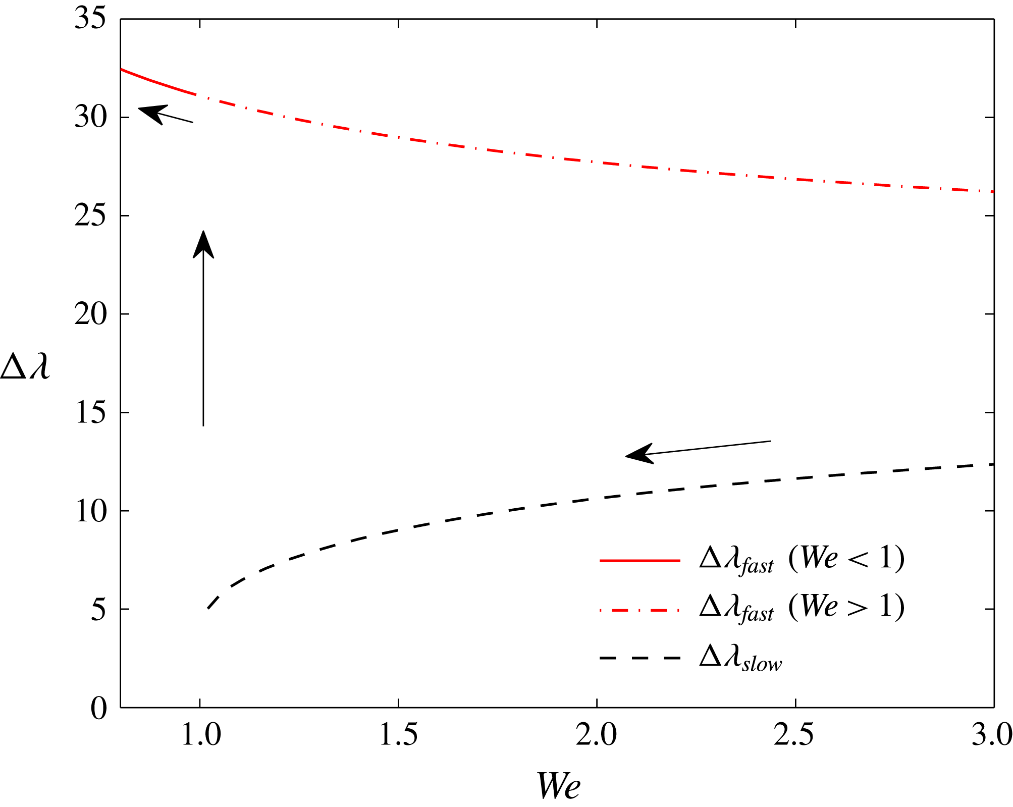
Due to the perfect reflecting character of the inlet boundary, any disturbance propagating towards the upstream direction is only reflected and its asymptotic behaviour will be the same as that of the disturbances propagating on the downstream direction. As a consequence, two branches of spectra in supercritical cases and just one branch in subcritical cases are predicted. Hence, in the critical regime, when passing from subcritical to supercritical conditions, the appearance of another branch of the spectrum, associated with the slower characteristic curve, is expected, whilst the faster branch should be continuous.
Such predictions will be confirmed by the subsequent spectral analysis, which is further corroborated by numerical simulations.
In order to have a global system perspective, the equations can be rearranged by introducing integral quantities depending on the sheet extension as a whole. After expressing the substantial derivative in explicit form, integrating (3.2) over the length of the sheet yields:
 $$\begin{eqnarray}\bar{H}{\displaystyle \frac{\text{d}^{2}\bar{\ell }}{\text{d}t^{2}}}+2{\displaystyle \frac{\text{d}\bar{\ell }}{\text{d}t}}+{\mathcal{K}}\bar{\ell }=\underbrace{-2{\displaystyle \frac{\text{d}}{\text{d}t}}\int _{0}^{1}x{\displaystyle \frac{\unicode[STIX]{x2202}\ell }{\unicode[STIX]{x2202}x}}\,\text{d}x-\left[U\left(1-\frac{1}{WeU}\right)\cdot {\displaystyle \frac{\unicode[STIX]{x2202}\ell }{\unicode[STIX]{x2202}x}}\right]_{0}^{1}}_{f_{i}},\end{eqnarray}$$
where
 $f_{i}$
represents the self-induced forcing acting on an elastic oscillator of stiffness
 ${\mathcal{K}}$
. According to the development of De Rosa et al. (Reference De Rosa, Girfoglio and de Luca2014), the following position has been made:
 $$\begin{eqnarray}\displaystyle \bar{H}=\int _{0}^{1}H\,\text{d}x & & \displaystyle\end{eqnarray}$$
and the boundary condition at the inlet location,
 $\ell (0)=0$
, has been considered. Quantities at the inlet and outlet boundaries are denoted with the subscripts 0 and 1, respectively. This notation will be used hereafter for all the boundary quantities. Equation (3.6) exhibits a strict analogy with the motion equation of an elastic oscillator, where
 $\bar{H}$
denotes the mass of the liquid sheet and
 ${\mathcal{K}}$
is the equivalent spring stiffness of the enclosure air. A proper manipulation led to extracting a damping term. In the supercritical regime the condition
 $\unicode[STIX]{x2202}\ell /\unicode[STIX]{x2202}x|_{0}=0$
is enforced. At large times one can expect the emergence of a characteristic mode which corresponds to the global response of the system behaving as a forced–damped oscillator. Of course, since the oscillator works in driven regime, the oscillation period does not corresponds to the natural frequency of oscillation and, in general, it cannot be determined in analytical closed form.
To sum up the nappe dynamics consists in the mutual interaction of the centreline local deflection with the compliant air chamber which behaves as a spring acting on the average sheet deflection. Equation (3.2) shows that the local deflection is forced by the global reaction of the spring, whilst the dynamics of the global spring–mass oscillator is driven by a combination of local displacement values, as described by (3.6). This interpretation has been carefully verified by De Rosa et al. (Reference De Rosa, Girfoglio and de Luca2014) who monitored frequency and phase of the forcing term
 $f_{i}$
in connection with spring–mass natural frequency and its phase lag. Self-forced spring–mass behaviour was experimentally found by Binnie (Reference Binnie1974), Sato et al. (Reference Sato, Miura, Nagamine, Morii and Ohkubo2007), as well as Brunet et al. (Reference Brunet, Clanet and Limat2004) in the context of oscillating water bells.
4 Linear stability analysis
A comprehensive methodology to analyse the asymptotic global behaviour of the nappe dynamics lies in formulating a boundary value eigenvalues problem. This can be conveniently carried out starting from (2.33)–(2.34) and enforcing the global temporal modes position, i.e. assuming the following form of the disturbances:
 $\ell (x,t)=\hat{\ell }(x)\cdot \text{e}^{\unicode[STIX]{x1D706}t}$
and
 $v(x,t)=\hat{v}(x)\cdot \text{e}^{\unicode[STIX]{x1D706}t}$
, where
 $\hat{\ell }$
and
 $\hat{v}$
are eigenfunctions and
 $\unicode[STIX]{x1D706}$
is the complex eigenvalue. This allows the governing equations to be recast into the following matrix form
 $$\begin{eqnarray}\unicode[STIX]{x1D706}\left(\begin{array}{@{}c@{}}\displaystyle \hat{\ell }\\ \displaystyle \hat{v}\end{array}\right)={\mathcal{A}}\left(\begin{array}{@{}c@{}}\displaystyle \hat{\ell }\\ \displaystyle \hat{v}\end{array}\right),\end{eqnarray}$$
where the spatial operator is
 $$\begin{eqnarray}\displaystyle {\mathcal{A}}\equiv \left(\begin{array}{@{}cc@{}}\displaystyle -U\cdot {\mathcal{D}} & \displaystyle -{\mathcal{I}}\\ \displaystyle \frac{U}{We}\cdot {\mathcal{D}}^{2}-{\displaystyle \frac{{\mathcal{K}}}{H}}\int _{0}^{1}\,\text{d}x & \displaystyle -U\cdot {\mathcal{D}}\end{array}\right), & & \displaystyle\end{eqnarray}$$
with
 ${\mathcal{I}}$
denoting the identity operator, and
 ${\mathcal{D}}$
and
 ${\mathcal{D}}^{2}$
the first and the second spatial derivatives, respectively.
Eigenvalues and eigenfunctions are numerically computed by means of a Chebyshev collocation method in MATLAB environment, where both differential and integral terms are spectrally accurate.
As has already been anticipated, for inlet supercritical conditions,
 $We>1$
, the two boundary conditions are both imposed at the inlet section, i.e.
 $$\begin{eqnarray}\displaystyle & \displaystyle \hat{\ell }(0)=0 & \displaystyle\end{eqnarray}$$
 $$\begin{eqnarray}\displaystyle & \displaystyle \left.\frac{\unicode[STIX]{x2202}\hat{\ell }}{\unicode[STIX]{x2202}x}\right|_{0}=0. & \displaystyle\end{eqnarray}$$
On the contrary, for the subcritical inlet,
 $We<1$
, due to the upstream directed wave characteristic velocity
 $U-\sqrt{U/We}$
, the perfectly reflecting conditions
 $\hat{\ell }(0)=0$
can only be retained at the inlet boundary. On the other hand, the eigenvalues equation becomes singular and the condition really removing this singularity constitutes the required second boundary condition.
4.1 Singularity treatment
Enforcing the temporal modes position on (3.1) leads to the following equation
 $$\begin{eqnarray}\frac{\text{d}}{\text{d}x}\left[\left(U-\frac{1}{We}\right)\frac{\text{d}\hat{\ell }}{\text{d}x}\right]+2\unicode[STIX]{x1D706}\frac{\text{d}\hat{\ell }}{\text{d}x}+\unicode[STIX]{x1D706}^{2}\frac{1}{U}\hat{\ell }=-{\mathcal{K}}\bar{\hat{\ell }}.\end{eqnarray}$$
This is a Sturm–Liouville-like eigenvalue integro-differential equation. It is singular since the second-order term coefficient vanishes at the location where the flow, accelerating due to gravity, reaches a critical velocity equal to
 $1/We$
. This singularity has been removed by developing the following procedure.
Integrating (4.5) from the inlet location to the generic location
 $x$
and resolving for
 $\unicode[STIX]{x2202}\hat{\ell }/\unicode[STIX]{x2202}x$
(by taking into account the kinematic boundary condition), yield an expression for the local slope of the sheet centreline, which depends on the slope value at the inlet location
 $$\begin{eqnarray}\frac{\unicode[STIX]{x2202}\hat{\ell }}{\unicode[STIX]{x2202}x}=\frac{-{\mathcal{K}}x\bar{\hat{\ell }}-\unicode[STIX]{x1D706}\hat{\ell }-\unicode[STIX]{x1D706}\displaystyle \left.\int _{0}^{x}\frac{\hat{v}}{U}\,\text{d}\unicode[STIX]{x1D709}+\left(1-\frac{1}{We}\right)\frac{\unicode[STIX]{x2202}\hat{\ell }}{\unicode[STIX]{x2202}x}\right|_{0}}{U-\displaystyle \frac{1}{We}}.\end{eqnarray}$$
It has already been stated that in supercritical conditions, since the perturbations do not travel upstream, it is generally assumed
 $\unicode[STIX]{x2202}\hat{\ell }/\unicode[STIX]{x2202}x|_{0}=0$
, as observed also experimentally by Finnicum et al. (Reference Finnicum, Weinstein and Rushak1993) in the steady state situation. On the other hands, note that in a supercritical regime the denominator never vanishes in any location. The scenario changes dramatically in subcritical regime since at the critical station where the local Weber number is unity, the denominator of (4.6) vanishes. Since for inlet Weber numbers weakly less than unity the sheet can survive without rupture, one can hypothesize that the sheet assumes an initial slope which is able to eliminate this singularity (Finnicum et al.
Reference Finnicum, Weinstein and Rushak1993). The idea is to evaluate the initial slope
 $\unicode[STIX]{x2202}\hat{\ell }/\unicode[STIX]{x2202}x|_{0}$
which nullifies the numerator of (4.6) and to substitute it into the equation itself, so as to obtain an undetermined ratio. We find
 $$\begin{eqnarray}\left.\frac{\unicode[STIX]{x2202}\hat{\ell }}{\unicode[STIX]{x2202}x}\right|_{0}=\frac{{\mathcal{K}}x_{s}\bar{\hat{\ell }}+\unicode[STIX]{x1D706}\hat{\ell }(x_{s})+\unicode[STIX]{x1D706}\displaystyle \int _{0}^{x_{s}}\frac{\hat{v}}{U}\,\text{d}\unicode[STIX]{x1D709}}{1-\displaystyle \frac{1}{We}}\end{eqnarray}$$
and the relationship of the slope at any generic station
 $x$
assumes the form
 $$\begin{eqnarray}\frac{\unicode[STIX]{x2202}\hat{\ell }}{\unicode[STIX]{x2202}x}=\frac{{\mathcal{K}}(x_{s}-x)\bar{\hat{\ell }}+\unicode[STIX]{x1D706}\hat{\ell }(x_{s})-\unicode[STIX]{x1D706}\hat{\ell }(x)-\unicode[STIX]{x1D706}\displaystyle \int _{x_{s}}^{x}\frac{\hat{v}}{U}\,\text{d}\unicode[STIX]{x1D709}}{U-\displaystyle \frac{1}{We}},\end{eqnarray}$$
where
 $x_{s}$
is the location where
 $U=1/We$
, namely where
 $We_{l}=1$
, given by
 $$\begin{eqnarray}x_{s}=\frac{Fr(1-We^{2})}{2We^{2}}.\end{eqnarray}$$
Applying de L’Hôpital’s rule allows us to calculate the singular limit as
 $$\begin{eqnarray}\left.\frac{\unicode[STIX]{x2202}\hat{\ell }}{\unicode[STIX]{x2202}x}\right|_{x_{s}}=\frac{-{\mathcal{K}}\bar{\hat{\ell }}-\unicode[STIX]{x1D706}We\cdot \hat{v}(x_{s})}{\unicode[STIX]{x1D706}+We/Fr}.\end{eqnarray}$$
In conclusion, for subcritical inlet, the boundary conditions to be enforced in solving the eigenvalue problem are expressed by (4.10) together with
 $\hat{\ell }(0)=0$
.
An analytical study of the singularity has been developed in order to provide further insights on the modal behaviour of the system. We will limit ourselves to stressing just some theoretical considerations which are useful in confirming theoretical results although, as will be seen, a complete analytical solution can be obtained, at least for certain values of the dimensionless parameters
 $We$
and
 $Fr$
. For our purposes, we neglect the pressure term in (4.5), the presence of which does not influence the singularity features, and we refer to the following equation (the first derivative which appears in (4.5) has been developed)
 $$\begin{eqnarray}\underbrace{U^{2}\left(1-\frac{1}{We_{l}}\right)}_{P}\frac{\text{d}^{2}\hat{\ell }}{\text{d}x^{2}}+\underbrace{(2U\unicode[STIX]{x1D706}+1)}_{Q}\frac{\text{d}\hat{\ell }}{\text{d}x}+\underbrace{\unicode[STIX]{x1D706}^{2}}_{R}\hat{\ell }=0.\end{eqnarray}$$
It is easily verified that the following conditions are satisfied:
 $$\begin{eqnarray}\displaystyle & \displaystyle P(x_{s})=0 & \displaystyle\end{eqnarray}$$
 $$\begin{eqnarray}\displaystyle & \displaystyle \lim _{x\rightarrow x_{s}}(x-x_{s})\frac{Q}{P}=\frac{Fr}{We}\left(2\unicode[STIX]{x1D706}+We\right)\quad \text{(finite)} & \displaystyle\end{eqnarray}$$
 $$\begin{eqnarray}\displaystyle & \displaystyle \lim _{x\rightarrow x_{s}}(x-x_{s})^{2}\frac{R}{P}=0\quad \text{(finite)}. & \displaystyle\end{eqnarray}$$
Therefore, the singular abscissa can be classified as a regular singular point (Boyce & DiPrima Reference Boyce and DiPrima2008). According to the basic Frobenius theory (Bender & Orszag Reference Bender and Orszag1999), the solution to (4.11) around the singularity location can be expressed by means of the following series expansion:
 $$\begin{eqnarray}\hat{\ell }(x,s)=(x-x_{s})^{\unicode[STIX]{x1D6FC}}\mathop{\sum }_{n=0}^{\infty }a_{n}(x-x_{s})^{n}.\end{eqnarray}$$
Substituting the above position in (4.11) and imposing the equality of same-order terms lead us to (for
 $n=0$
) the following indicial equation
 $$\begin{eqnarray}a_{0}\left[\frac{1}{We}\unicode[STIX]{x1D6FC}(\unicode[STIX]{x1D6FC}-1)+\left(\frac{1}{We}+\frac{2}{We^{2}}\unicode[STIX]{x1D706}\right)\unicode[STIX]{x1D6FC}\right]=0.\end{eqnarray}$$
Since by definition
 $a_{0}\neq 0$
, equation (4.16) yields
 $$\begin{eqnarray}\unicode[STIX]{x1D6FC}_{1}=0\quad \unicode[STIX]{x1D6FC}_{2}=-\frac{2Fr\unicode[STIX]{x1D706}}{We}.\end{eqnarray}$$
The structure of the solution depends mainly on the value assumed for the difference of the roots
 $\unicode[STIX]{x1D6FC}_{1}-\unicode[STIX]{x1D6FC}_{2}$
(particular cases occur when
 $\unicode[STIX]{x1D6FC}_{1}$
and
 $\unicode[STIX]{x1D6FC}_{2}$
are equal, or differ by an integer, and the singular equation has a second solution involving a logarithmic term). In the present analysis, this characteristic difference is given by
 $$\begin{eqnarray}\unicode[STIX]{x1D6FC}_{1}-\unicode[STIX]{x1D6FC}_{2}=\frac{2Fr\unicode[STIX]{x1D706}}{We}.\end{eqnarray}$$
Therefore, the particular cases can be excluded and the solution to the singular differential equation is given by the linear combination of two Frobenius series
 $$\begin{eqnarray}\hat{\ell }(x,s)=C_{1}\mathop{\sum }_{n=0}^{\infty }a_{n,1}(x-x_{s})^{n}+C_{2}(x-x_{s})^{-(2\unicode[STIX]{x1D706}Fr/We)}\mathop{\sum }_{n=0}^{\infty }a_{n,2}(x-x_{s})^{n},\end{eqnarray}$$
where
 $C_{1}$
and
 $C_{2}$
are constants to be determined by taking into account the boundary conditions. Note that, being
 $\unicode[STIX]{x1D6FC}_{1}=0$
, the first Frobenius series reduces to a standard power series expansion (Taylor series).
It is worthwhile analysing the convergence properties of the series expansion (4.19). Equation (4.11) shows another regular singular point at
 $U=0$
(
 $\bar{x}=-Fr/2$
). The radius of convergence of the series (4.19) is smaller than or equal to the distance between
 $x_{s}$
and the nearest singular point
 $\bar{x}$
. Therefore, the series expansion (4.19) converges to the eigenvalues problem (4.11) solution at least at each station
 $x\in ]\!-Fr/2,-Fr/2+Fr/We^{2}\! [$
.
Note that the physical domain extends from 0 to 1; therefore, we can conclude that for
 $-Fr/2+Fr/We^{2}>1$
and, so, for
 $$\begin{eqnarray}We<\sqrt{\frac{2}{2/Fr+1}}\end{eqnarray}$$
the series (4.19) represents, in principle, the complete analytic solution to the singular eigenvalues problem (4.11). The series, therefore, is not uniformly convergent, which means that the analytic solution of limited application. On the other hand, the singular location
 $\bar{x}=-Fr/2$
is not physically interesting because it is located outside the sheet domain for each
 $Fr$
and, therefore, it does not need any special treatment.
With reference to the expansion (4.19), the boundedness condition of
 $\text{d}\hat{\ell }/\text{d}x$
in
 $x_{s}$
can be formulated as
 $$\begin{eqnarray}\lim _{x\rightarrow x_{s}}(x-x_{s})^{n-1-(2Fr\unicode[STIX]{x1D706}_{r}/We)}<\infty \quad \forall n.\end{eqnarray}$$
Of course the boundedness condition affects the part real of the derivative of any series term only, because the imaginary one
 $$\begin{eqnarray}\cos \left(\frac{-2Fr\unicode[STIX]{x1D706}_{i}}{We}\log |x-x_{s}|\right)+\text{i}\sin \left(\frac{-2Fr\unicode[STIX]{x1D706}_{i}}{We}\log |x-x_{s}|\right)\end{eqnarray}$$
is oscillating and results in being unconditionally bounded for
 $x\rightarrow x_{s}$
.
Equation (4.21) yields
 $$\begin{eqnarray}\unicode[STIX]{x1D706}_{r}<-\frac{We}{2Fr}\end{eqnarray}$$
and therefore we can conclude that, in a critical regime, not only is the spectrum unconditionally stable for each
 $We$
and
 $Fr$
, but it is subjected to the constraint of the maximum achievable growth rate. In other words, the growth rate is bounded. As will be seen, the numerical results will confirm this prediction.
4.2 Numerical simulation
To corroborate the asymptotic modal analysis, numerical simulations of the governing equations system (2.33)–(2.34) have also been carried out, by means of a standard finite-difference discretization. The initial condition is constituted by a compact support function satisfying the prescribed boundary conditions, namely a Gaussian-like pulse for the perturbed centreline of nappe, properly localized upstream or downstream of the singularity station depending on the flow regime nature, subcritical or supercritical, respectively. No perturbation in lateral velocity fluctuation
 $v$
is considered here. Among the various possibilities analysed during the numerical tests, the most convenient numerical procedure appeared to be that based on the direct integration of the system of two equations (2.33)–(2.34). Bearing in mind the wave nature of the expected solution, we formally imposed just the reflecting condition,
 $\ell (0)=0$
, on (2.33), the free-outflow condition at the right boundary being self-guaranteed. It should be stressed that, as a consequence, at the inlet station the equation (2.33) is implicitly enforced as
 $v=U(\unicode[STIX]{x2202}\ell /\unicode[STIX]{x2202}x)$
. No particular treatment has been added for the specific subcritical or supercritical regimes.
The numerical simulation of the spatio-temporal partial-derivative equations did not need any special trick for the presence of the singularity in subcritical regime. The large time simulation usually agrees perfectly with the corresponding eigenfunction from the modal analysis.
5 Results
Computed modes and oscillation frequencies of the liquid sheet occurring in the various flow regimes of
 $We$
number will be presented in this section, with initial emphasis on the critical region, i.e.
 $We=O(1)$
. In order to make calculations with physically relevant parameters, we first hypothesized to work with a water–air fluid couple (
 $\unicode[STIX]{x1D70E}=0.073~\text{N}~\text{m}^{-1}$
,
 $\unicode[STIX]{x1D70C}_{l}=1000~\text{kg}~\text{m}^{-3}$
,
 $\unicode[STIX]{x1D6FE}=1.4$
) at a base cavity pressure
 $P_{a}^{\star }=10^{5}~\text{Pa}$
(and standard ambient temperature), and we assumed also
 $Fr=O(1)$
. Choosing the cavity height
 $L^{\star }=0.15~\text{m}$
(of the same order as the values reported by de Luca (Reference de Luca1999) and by Finnicum et al. (Reference Finnicum, Weinstein and Rushak1993), equal to 0.275 m and 0.305 m, respectively), and the slit width
 $H_{in}^{\star }=0.1\times 10^{-3}~\text{m}$
(for instance, Finnicum et al. (Reference Finnicum, Weinstein and Rushak1993) realized an inlet thickness of approximately
 $0.25\times 10^{-3}~\text{m}$
), yields a sheet inlet velocity of
 $U_{in}^{\star }=1.2~\text{m}~\text{s}^{-1}$
(as made by Binnie Reference Binnie1974; Sato et al.
Reference Sato, Miura, Nagamine, Morii and Ohkubo2007; Mori et al.
Reference Mori, Nagamine, Ito and Sato2012). Thus, one can achieve both
 $Fr\simeq 1$
and
 $We\simeq 1$
, with
 $\unicode[STIX]{x1D700}$
being equal to
 $0.67\times 10^{-3}$
. Finally, by taking into account that
 $W^{\star }/L^{\star }$
ranges typically from 0.2 (Schmid & Henningson Reference Schmid and Henningson2002) to 1 (Binnie Reference Binnie1974), typical values of
 ${\mathcal{K}}=O(10^{6})$
and
 ${\mathcal{K}}=O(10^{5})$
, respectively, are obtained. Furthermore, we will see also that for a typical geometrical configuration of Binnie (Reference Binnie1974), the critical regime can be obtained also with a relatively low inlet velocity, thus having simultaneously
 $Fr=0.077$
and
 ${\mathcal{K}}=5\times 10^{5}$
.
Oscillation frequencies will be compared with experimental data from the literature which, are available in the supercritical regime at relatively high
 $We$
numbers. In critical or subcritical regimes experimental results refer to geometrical configurations interacting on an unconfined ambient through both interfaces. Indeed, experimental findings are available in the critical regime for nominally axisymmetric liquid bells investigated by Brunet et al. (Reference Brunet, Clanet and Limat2004), who adopted inlet boundary conditions allowing modulations of the circumference on which the bell intersects the solid ceiling. These data are clearly not suitable for making comparisons with the behaviour of the flat configuration here analysed. In the model of Brunet et al. (Reference Brunet, Clanet and Limat2004) oscillations are produced by surface tension-driven pressure variations (due to the bell deformation), whilst in the present sheet case oscillations are produced by isentropic pressure variations due to the displacement of the sheet centreline.
5.1 Highlights of numerical simulations
Systematic numerical simulations of spatio-temporal evolution of the interface deflection have been carried out, starting from an initial instant when a particular perturbation, a Gaussian-like bump, is imposed on the interface. No initial disturbance on the lateral velocity perturbation
 $v$
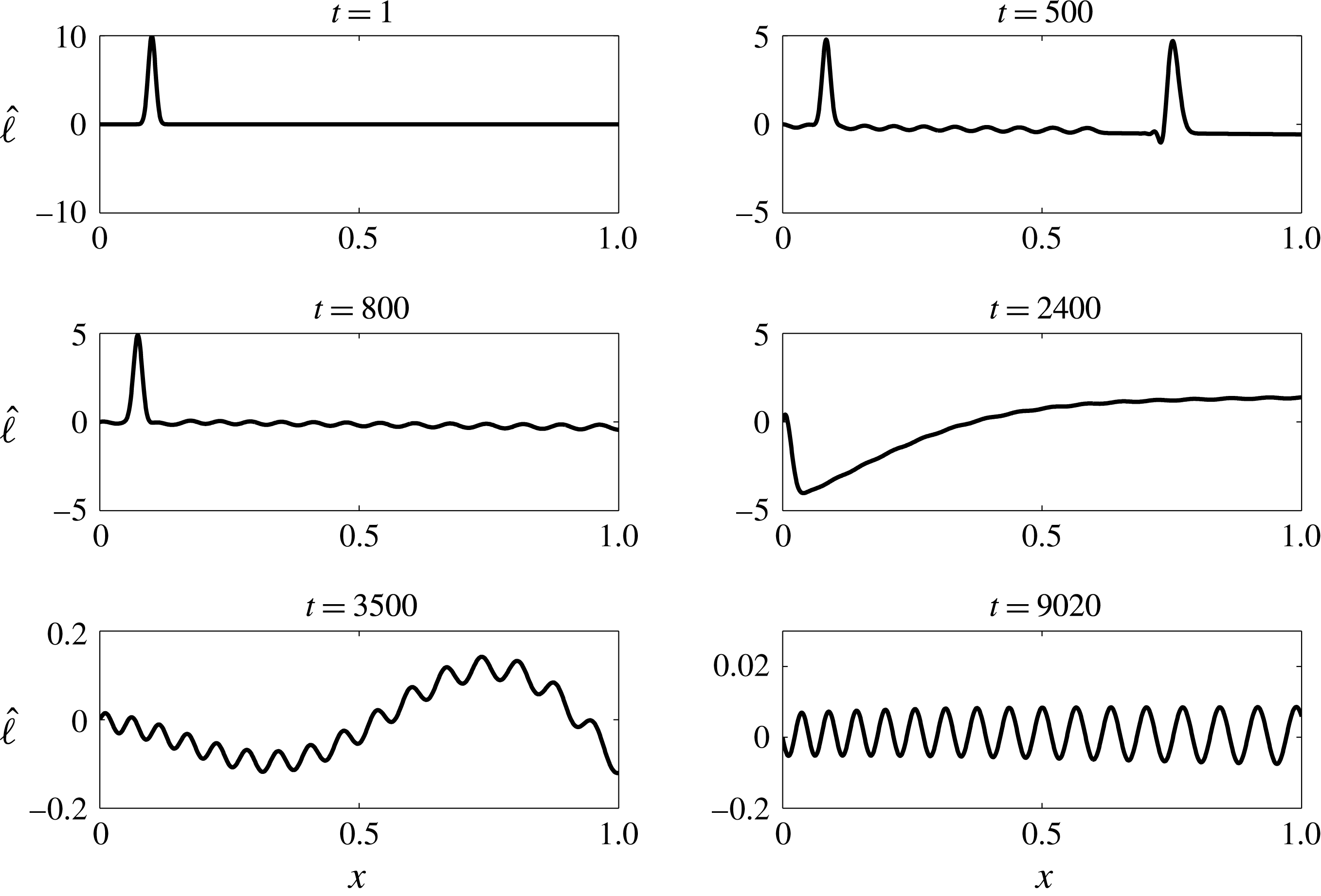
has been considered. Due to the lack of experimental data in the subcritical regime, the numerical simulations have been utilized to validate the eigenvalues analysis, especially the treatment used to remove the singularity. A broad comparison with experimental results in the supercritical regime will be reported below. The temporal panels shown in figure 2 refer to the evolution computed for the subcritical case of
 $We=0.82$
with
 ${\mathcal{K}}=5\times 10^{4}$
,
 $\unicode[STIX]{x1D700}=6.7\times 10^{-4}$
, and to a bump disturbance initially located at
 $x=0.1$
, i.e. in the subcritical region
 $0<x<x_{s}$
, here resulting in
 $x_{s}=0.24$
(4.9). Note also that other simulations, not shown herein, revealed that the asymptotic deflection eventually reached by the sheet is not influenced by the initial position of the disturbance. The panels reported in figure 2 show an initial bump splitting into two parts, one travelling rightwards and being rapidly expelled, the other one travelling leftwards, where both have the expected velocities. The reflection of the left part on the inlet boundary at
 $x=0$
generates the temporary establishment of a low wavenumber mode which is rapidly characterized by the appearance of shorter wavelength ripples. At large times a travelling wave, exhibiting an almost regular structure with a wavenumber of approximately
 $k=15$
, is eventually established. Details about the transition from an initial impulse to the rise of capillary waves are presented in the movie, provided as supplementary material available at https://doi.org/10.1017/jfm.2017.241.


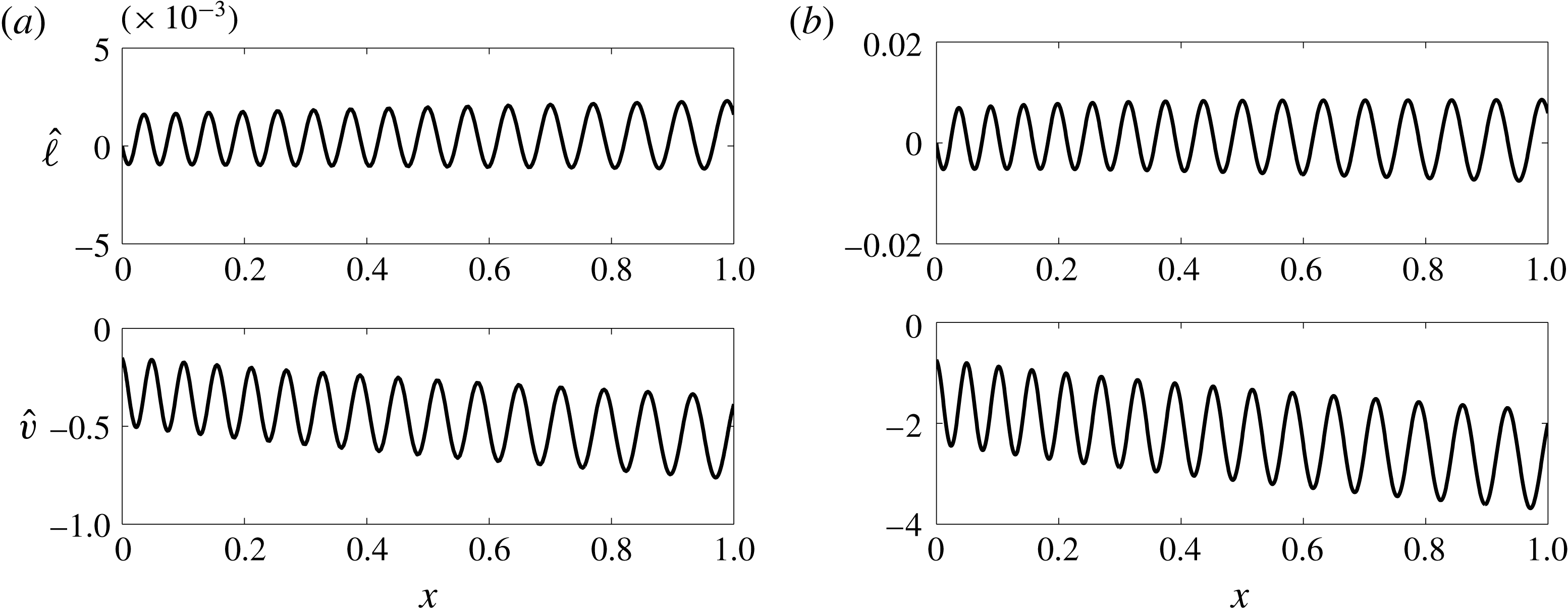
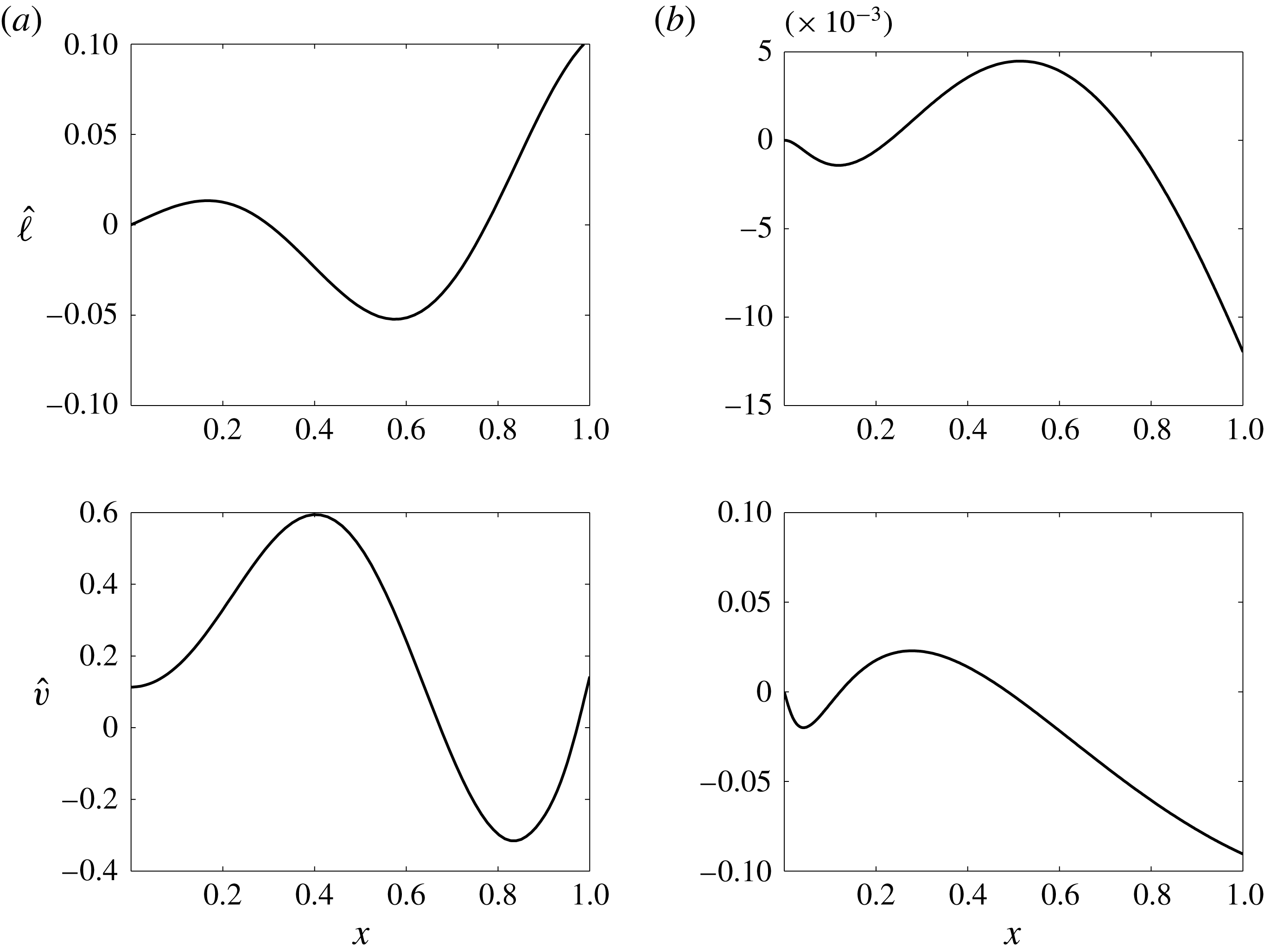
A comparison of large time sheet centreline deflection and lateral velocity between eigenmodes (a) and numerical simulations (b) is reported in figure 3, referring to the same parameters as the panels of the previous figure. The physical relevance of the result will be addressed later on, when discussing the shape of modes observed in actual experimental rigs.


The above comparisons appear quite satisfactory. In particular, note the perfect agreement of the two solutions near the singularity station
 $x_{s}=0.24$
, showing that the treatment of the singularity worked successfully in the spectral analysis. A further finding is the confirmation of the travelling wave feature of the solution; as was verified in a wide range of flow conditions, the wave velocity satisfies the following relationship to within good accuracy
 $$\begin{eqnarray}\bar{a}=\frac{\unicode[STIX]{x1D706}_{i}}{2\unicode[STIX]{x03C0}k},\end{eqnarray}$$
with
 $\unicode[STIX]{x1D706}_{i}$
indicating the disturbance circular frequency (i.e. the imaginary coefficient of eigenvalue) and
 $k$
the wavenumber, which can be evaluated by inspecting the eigenfunctions. The average
 $\bar{a}$
velocity is, on the other hand, directly evaluated as
 $\bar{a}=1/t_{cross}$
, where the crossing time is
 $$\begin{eqnarray}t_{cross}=\int _{0}^{1}{\displaystyle \frac{\text{d}x}{U\pm \displaystyle \sqrt{\frac{U}{We}}}}.\end{eqnarray}$$
5.2 Analysis of critical regime
Some significant results of the spectral analysis for
 $We$
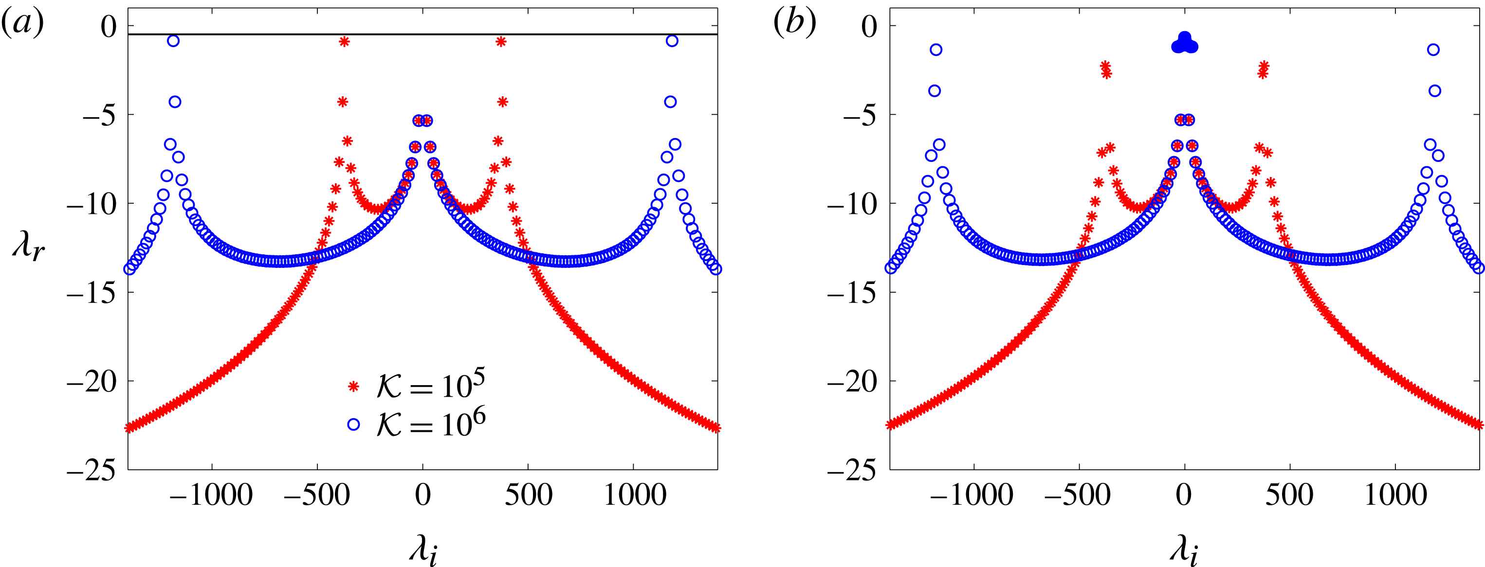
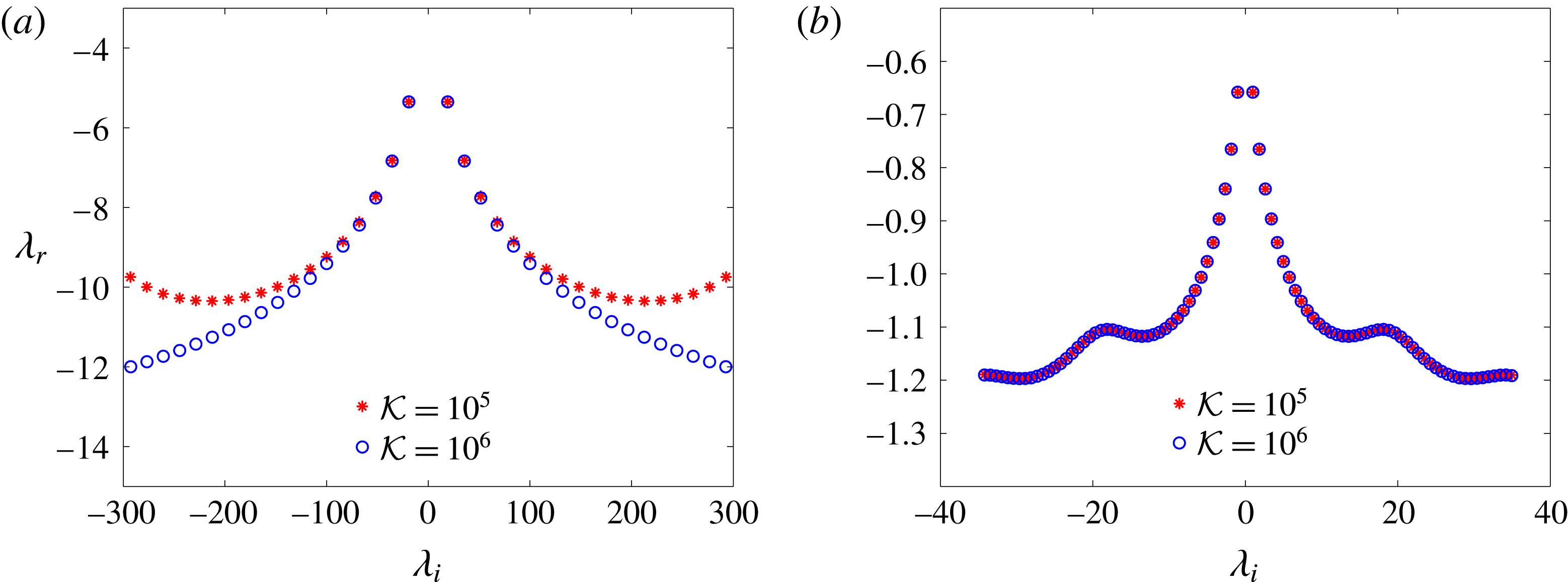
around unity will be hereafter presented. Figure 4 compares spectra obtained in subcritical (
 $We=0.98$
) and supercritical (
 $We=1.02$
) regimes for
 $Fr=1$
and two typical values of the air stiffness,
 ${\mathcal{K}}=10^{5}$
and
 ${\mathcal{K}}=10^{6}$
. As predicted before, the subcritical regime (for
 $We=0.98$
it is
 $x_{s}=0.021$
) is characterized by one branch only (associated with the faster travelling wave with velocity
 $U+\sqrt{U/We}$
), constituted by two symmetrical parts exhibiting outer cusp-point maxima, as well as local maxima (independent of
 ${\mathcal{K}}$
) represented by the inner pair of eigenvalues. The configurations reported in figure 4(a) are stable. Note also that, as already extensively discussed by De Rosa et al. (Reference De Rosa, Girfoglio and de Luca2014), according to the damped spring–mass model driven by the self-induced forcing
 $f_{i}$
of (3.6), the frequency of the less stable eigenvalue approximately scales with
 $\sqrt{{\mathcal{K}}}$
(of course in the driven regime it coincides with that of the forcing term). Another characteristic frequency is represented by the constant spacing
 $\unicode[STIX]{x0394}\unicode[STIX]{x1D706}_{i}$
of the imaginary parts of the eigenvalues which is related to the crossing time by
 $\unicode[STIX]{x0394}\unicode[STIX]{x1D706}_{i}\approx 2\unicode[STIX]{x03C0}/t_{cross}$
. The horizontal continuous line of figure 4(a) is the theoretical upper bound of inequality (4.23), which in the present case yields
 $\unicode[STIX]{x1D706}_{r}<-0.49$
and therefore it is satisfied. Figure 4(b) reports spectra for
 $We=1.02$
and the same values of
 ${\mathcal{K}}$
as the previous figure 4(a). Thus, the analysis of these two spectra sheds light on the critical region. The major feature is that, on the one the presence of a part of a branch representing the parametric continuation of the analogous branch found for
 $We=0.98$
is noted, on the other a new nucleus of eigenvalues having growth rate weakly less than zero clearly arises. The new nucleus of eigenvalues is to be ascribed to the travelling waves with velocity
 $U-\sqrt{U/We}$
and to their interference with low-frequency eigenvalues associated with the faster waves with velocity
 $U+\sqrt{U/We}$
. This last finding can be better appreciated by looking at figure 5(a,b), depicting the close-up views of the previous figures 4(a) and 4(b), respectively. It is very important to point out that in the above pictures the frequency scale is extended up to 1500 for the sake of completeness only, but values greater than approximately 300 are suspected not to have physical relevance because they are associated with high wavenumber modes, which are definitely damped by viscosity, while they also invalidate the assumption of thin sheet model. This issue will be raised again when discussing the comparison with experimental data in the supercritical regime. De Rosa et al. (Reference De Rosa, Girfoglio and de Luca2014) did not report this argument because their study was limited to a parametric investigation without further insights on the physical relevance of the higher-frequency modes.
Spectra for
 $Fr=1$
,
 $\unicode[STIX]{x1D700}=6.7\times 10^{-4}$
and selected
 ${\mathcal{K}}$
values. (a)
 $We=0.98$
, (b)
 $We=1.02$
.

Inner eigenvalues of spectra for
 $Fr=1$
,
 $\unicode[STIX]{x1D700}=6.7\times 10^{-4}$
and selected
 ${\mathcal{K}}$
values. (a)
 $We=0.98$
, (b)
 $We=1.02$
.

A first estimate of the viscous dissipation in short wavelength capillary ripples can be made by following the approach of Lighthill (Reference Lighthill1978), in particular with reference to the so-called internal dissipation mechanism, i.e. under the assumption that the viscous damping is limited to the wave amplitude, with the main flow field being irrotational. This approach, well established more recently by Joseph, Funada & Wang (Reference Joseph, Funada and Wang2007), is the basis also of the work of Longuet-Higgins (Reference Longuet-Higgins1997) dealing with capillary–gravity waves. Lighthill (Reference Lighthill1978) showed that the time constant
 $\unicode[STIX]{x1D70F}^{\star }$
for the exponential decay of surface waves of wavelength
 $\unicode[STIX]{x1D706}^{\star }$
is
 $$\begin{eqnarray}\unicode[STIX]{x1D70F}^{\star }=\frac{\unicode[STIX]{x1D706}^{\star ^{2}}}{16\unicode[STIX]{x03C0}^{2}\unicode[STIX]{x1D708}},\end{eqnarray}$$
with
 $\unicode[STIX]{x1D708}$
being the fluid kinematic viscosity.
As asserted by Joseph et al. (Reference Joseph, Funada and Wang2007), the wave attenuation can be evaluated by the distance (namely, the number of wavelengths) a wave travels before it decays by a certain amount, or, in other terms, by the number of oscillation periods,
 $T^{\star }$
, corresponding to a given decay amount. Thus, the quantity
 $\unicode[STIX]{x1D70F}^{\star }/T^{\star }$
measures the number of periods for the energy of sinusoidal waves to be reduced by a factor
 $e$
. By assuming a constant sheet thickness,
 $T^{\star }$
is given by
 $$\begin{eqnarray}T^{\star }=\unicode[STIX]{x1D706}^{\star }\sqrt{\frac{\unicode[STIX]{x1D70C}_{l}H_{in}^{\star }}{2\unicode[STIX]{x1D70E}}}\end{eqnarray}$$
and the following is finally obtained
 $$\begin{eqnarray}\unicode[STIX]{x1D70F}^{\star }/T^{\star }=\frac{1}{16\unicode[STIX]{x03C0}^{2}}\frac{1}{Oh}\frac{\unicode[STIX]{x1D706}^{\star }}{H_{in}^{\star }},\end{eqnarray}$$
where the Ohnesorge number is introduced as
 $$\begin{eqnarray}Oh=\unicode[STIX]{x1D708}\sqrt{\unicode[STIX]{x1D70C}_{l}/(2\unicode[STIX]{x1D70E}H_{in}^{\star })}.\end{eqnarray}$$
For standard values of the thermodynamic properties of water,
 $H_{in}^{\star }=10^{-3}~\text{m}$
and
 $\unicode[STIX]{x1D706}^{\star }/H_{in}^{\star }=10$
, one obtains
 $Oh=2.62\times 10^{-3}$
and
 $\unicode[STIX]{x1D70F}^{\star }/T^{\star }\simeq 24$
, while in the case of very short capillary ripples with
 $\unicode[STIX]{x1D706}^{\star }/H_{in}^{\star }=2$
the wave energy is expected to be reduced by a factor of
 $e$
in approximately five periods. This last prediction is consistent with the experimental findings of de Luca & Costa (Reference de Luca and Costa1997b
) who visualized sinuous waves produced by an obstacle on a free-falling sheet. It is also important to note that, in the presence of surfactant agents in the liquid, another attenuation effect has to be taken into account, i.e. the surface dissipation, that can exceed the internal dissipation, as discussed by Lighthill (Reference Lighthill1978) and experimentally approached by de Luca & Costa (Reference de Luca and Costa1997b
), who took advantage of a previous work of de Luca & Meola (Reference de Luca and Meola1995).
Figure 5(a) shows a detail of the lowest frequency eigenvalues (inner conjugate couples) calculated for
 $We=0.98$
(but not less stable eigenvalues for
 ${\mathcal{K}}=10^{5}$
and
 ${\mathcal{K}}=10^{6}$
), whilst figure 5(b) refers to the less stable supercritical (
 $We=1.02$
) eigenvalues (which are practically independent of
 ${\mathcal{K}}$
) and it shows in great detail the interference of modes. Although for
 $We=0.98$
the less stable modes are the higher-frequency ones scaling with
 $\sqrt{{\mathcal{K}}}$
, the physical considerations above lead us to think that the sheet shapes more likely observable in experiments are represented by the inner modes (i.e. local maxima); the same should occur in the supercritical condition of
 $We=1.02$
, where the inner modes are the less unstable, too. The difference lies in the fact that in the subcritical regime, the prevailing modes are of fast type, whilst in the supercritical regime they are of slow type. In fact, in the former case the order of magnitude of the other characteristic frequency of the system,
 $\unicode[STIX]{x0394}\unicode[STIX]{x1D706}_{i}\simeq 16.1$
, is associated with the crossing time of the fast mode, whilst in the latter one
 $\unicode[STIX]{x0394}\unicode[STIX]{x1D706}_{i}\simeq 0.75$
corresponds to the crossing time of the slow mode. The supercritical spectrum of figure 5(b) exhibits a wavy trend whose period is just
 $\unicode[STIX]{x0394}\unicode[STIX]{x1D706}_{i}\simeq 16.1$
, which evidences the interference between the modes. Finally, it is found that for
 $We=0.98$
the ratio of the frequency local peak to
 $\unicode[STIX]{x0394}\unicode[STIX]{x1D706}_{i}$
is approximately 1.18 and for
 $We=1.02$
this ratio is approximately 1.27. This occurrence is reminiscent of the integer-plus-one-quarter resonance criterion of forced transverse vibrations of the nappe string, already uncovered by De Rosa et al. (Reference De Rosa, Girfoglio and de Luca2014) in the absence of surface tension. This will be discussed in more detail later on, in connection with comparisons with experimental data available in the literature for the supercritical regime and can also be verified by inspecting the relevant eigenmodes.
The inner leading modes are presented in figure 6 for
 ${\mathcal{K}}=10^{5}$
and
 $Fr=1$
. Panels (a,b) refer to subcritical (
 $We=0.98$
) and supercritical (
 $We=1.02$
) regimes, respectively. Their comparison gives a picture of the sheet shape variation encountered when traversing the critical regime. The nappe oscillation frequency accordingly changes from 19.13 for the subcritical regime to 0.99 for the supercritical regime. This finding has to be validated through experimental investigations because of the absence of experimental data as regards the critical regime, and will be further discussed in the subsequent section.
Inner leading eigenfunctions for
 $Fr=1$
,
 ${\mathcal{K}}=10^{5}$
and
 $\unicode[STIX]{x1D700}=6.7\times 10^{-4}$
. (a)
 $We=0.98$
, (b)
 $We=1.02$
.

5.3 Insight into the supercritical regime
A rather detailed comparison of the present theoretical predictions with experiments undertaken by Binnie (Reference Binnie1974) and by Sato et al. (Reference Sato, Miura, Nagamine, Morii and Ohkubo2007) in the supercritical regime will be made in this section. Such a comparison will also represent the validation of the interpretation of the results found in the critical regime. The apparatus arrangement of Binnie (Reference Binnie1974) was very similar to that sketched in figure 1, concerning the formation of a thin sheet of water falling in air, in the presence of an air enclosure behind the sheet. Tests were carried out for various geometrical quantities and water flow rate values, so as to vary the Weber number (basically by increasing the water flow rate) in the range from 3.77 to 287 (the corresponding Froude number ranged from 0.28 to 7.69) and the dimensionless air stiffness
 ${\mathcal{K}}$
in the range from
 $10^{5}$
to
 $10^{3}$
, respectively. Sheet oscillation frequency was measured by means a stroboscope and the associated deformed centreline shape was detected indirectly by means of an optical method able to individuate positions half a wavelength apart on the shape. Binnie (Reference Binnie1974) predicted the modes associated with the natural frequencies of the nappe through a simplified physical model which did not include surface tension effects, and reported such modes for various testing conditions. With reference to his flow configuration, named A, with
 $We=95.9$
and
 ${\mathcal{K}}=5.87\times 10^{3}$
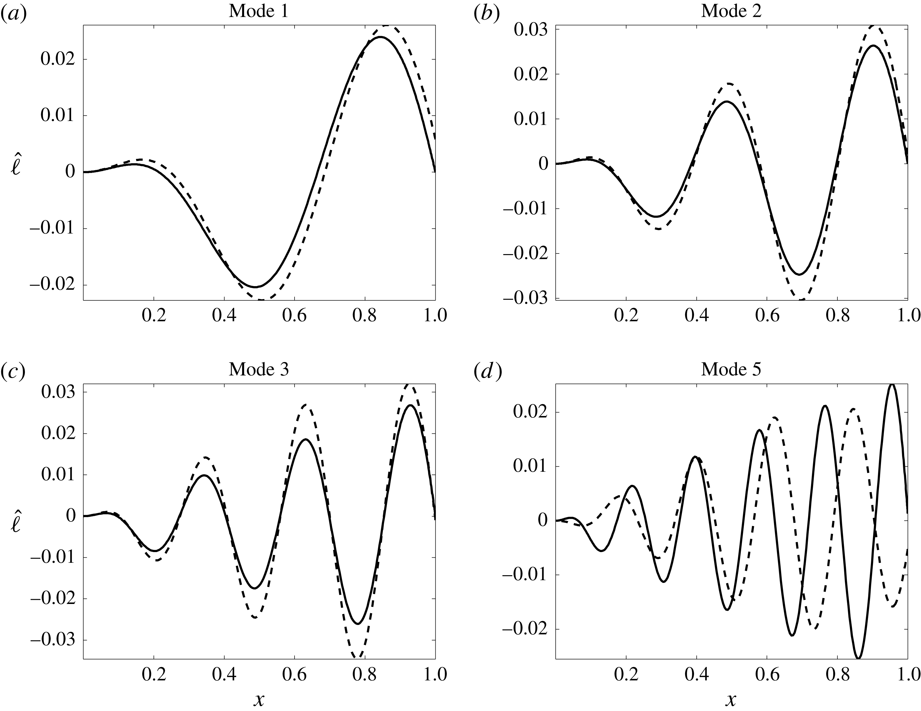
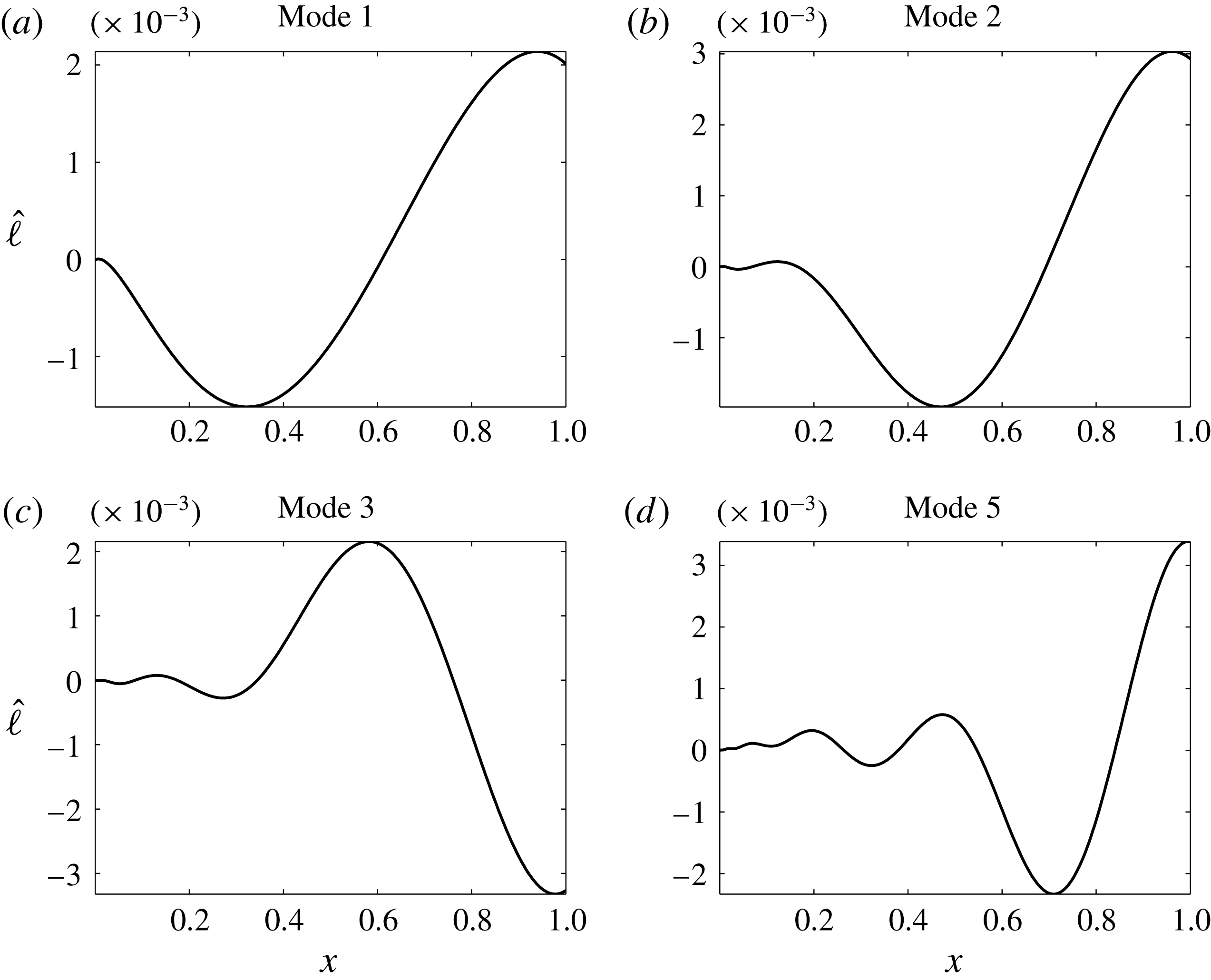
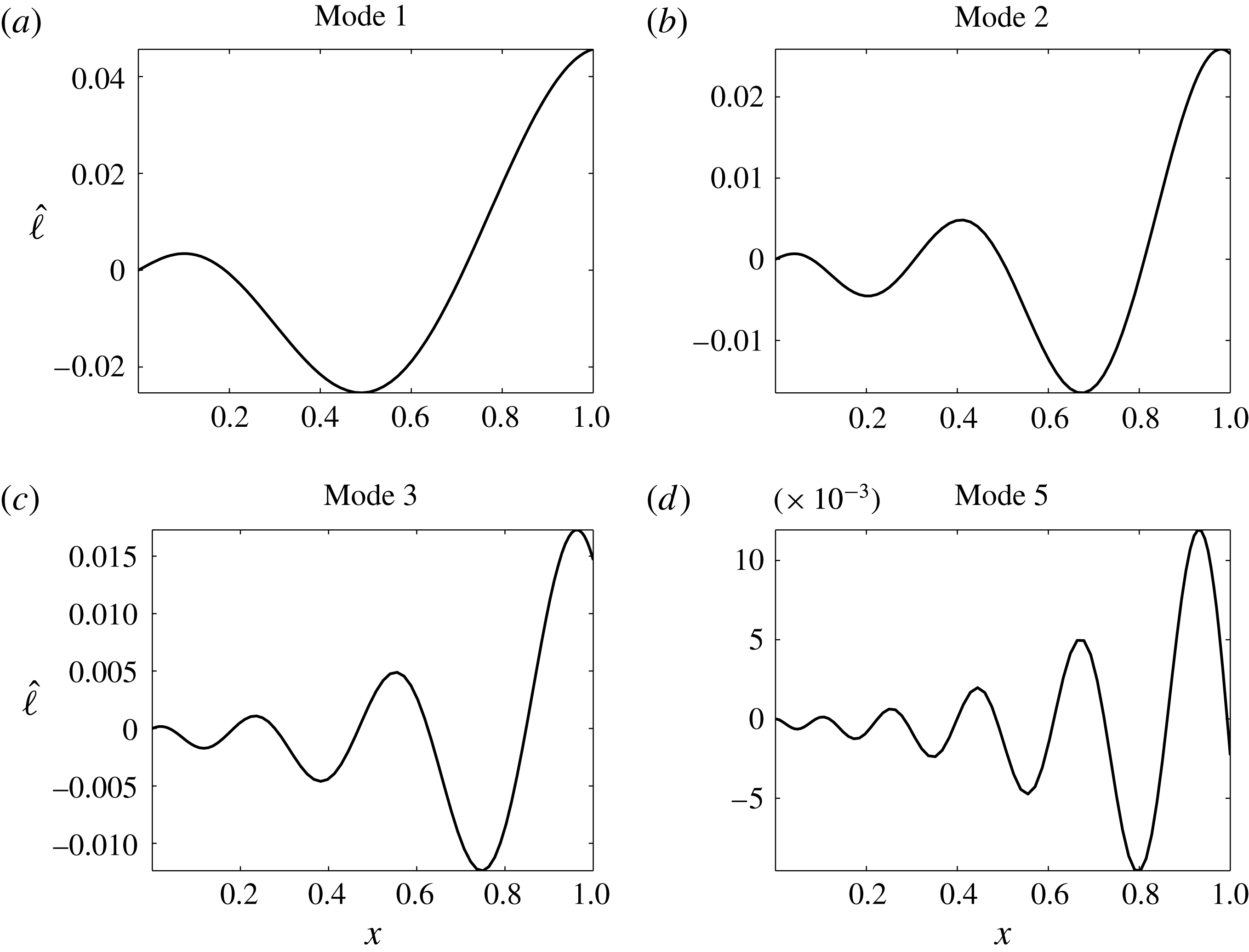
, panels (a–d) of figure 7 show the first, second, third and fifth mode, respectively, corresponding to less stable inner eigenvalues, as discussed before in regard to the critical regime. Such modes agree strictly with the predictions arising from Binnie’s theory which, in turn, agrees with his own experiments. Note that the peak frequency of the most unstable mode, namely the spring–mass frequency scaling with
 $\sqrt{{\mathcal{K}}}$
, equal to approximately 80 (namely 154 Hz), was not observed in the experiment; on the contrary, the fifth inner mode was detected in this configuration.
First, second, third and fifth eigenmodes for test A of Binnie (Reference Binnie1974) (
 $We=95.9$
,
 $Fr=7.69$
,
 ${\mathcal{K}}=5.87\times 10^{3}$
,
 $\unicode[STIX]{x1D700}=7.6\times 10^{-4}$
); the continuous lines refer to the present model, while the dashed lines refer to the Binnie’s model not including the surface tension.

A comparison between frequencies observed experimentally by Binnie (Reference Binnie1974) and calculated by the present physical model is shown in table 1. The tests from A to D refer to the same geometrical configuration, while in test F a wider nozzle width was used to work with a higher liquid velocity. Table 1 shows a quite good agreement between frequencies observed in experiments,
 $f_{e}^{\ast }$
, measured in Hertz, and frequencies evaluated numerically,
 $f_{n}^{\ast }$
, by the present analysis. Note that Binnie (Reference Binnie1974) too made a comparison between measured and calculated (via his simplified model) frequencies,
 $f_{b}^{\ast }$
, and attributed the discrepancy of the data to the difficulty in measuring correctly the liquid inlet velocity. In any case, the present comparison is better than Binnie’s. From Binnie’s experiments it is evident that the nappe always oscillates at lower frequencies corresponding to inner modes (which are all stable) of the spectrum, because higher-frequency modes are most likely damped by viscosity. The order of the observed mode cannot be predicted, of course, by the present theory and no explanation in this respect was furnished by the author of the experiments.
Comparison with experiments of Binnie (Reference Binnie1974);
 $f_{e}^{\ast }$
is the observed frequency,
 $f_{n}^{\ast }$
is the frequency predicted by the present analysis,
 $f_{b}^{\ast }$
is the frequency computed using Binnie’s model.

Comparison with experiments of Sato et al. (Reference Sato, Miura, Nagamine, Morii and Ohkubo2007);
 $f_{e}^{\ast }$
is the observed frequency,
 $f_{n}^{\ast }$
is the frequency predicted by the present analysis,
 $f_{b}^{\ast }$
is the frequency computed using Binnie’s model.

Another systematic comparison has been made with reference to experimental tests of Sato et al. (Reference Sato, Miura, Nagamine, Morii and Ohkubo2007), who carried out nappe shape visualizations and oscillation frequency measurements on an apparatus similar to that used by Binnie (Reference Binnie1974). However, Sato et al. (Reference Sato, Miura, Nagamine, Morii and Ohkubo2007) made direct visualizations by using a high-speed camera and compared observed frequencies with pressure fluctuations in the closed chamber behind the nappe. Table 2 refers to data points corresponding to the smallest slit width considered by the above authors. For this series of tests the agreement between measured frequencies
 $f_{e}^{\ast }$
and estimated frequencies
 $f_{n}^{\ast }$
is satisfactorily strict. Again one should note that the (stable) modes selected by the flow system do not correspond to frequencies of the order of
 $\sqrt{{\mathcal{K}}}$
, but to much lower values which are predicted by the inner eigenvalues. This point was outlined by Sato et al. (Reference Sato, Miura, Nagamine, Morii and Ohkubo2007) who, furthermore, pointed out that ‘the generated frequencies remain the same even when the chamber width (i.e.
 $W^{\ast }$
) was considerably changed’; in other words, they noted experimentally that the inner modes are independent of
 ${\mathcal{K}}$
, as confirmed by the present theoretical analysis.
Both Binnie (Reference Binnie1974) and Sato et al. (Reference Sato, Miura, Nagamine, Morii and Ohkubo2007) measurements gave evidence of the integer-plus-one-quarter resonance criterion, which is fulfilled by the present analysis. In the experimental investigation reported by Schmid & Henningson (Reference Schmid and Henningson2002), on the contrary, the nappe is seen to oscillate at the frequency corresponding to the base flow falling time, although from their theoretical analysis it is evident that the lowest frequency is approximately 1.28 times of that corresponding to the falling time.
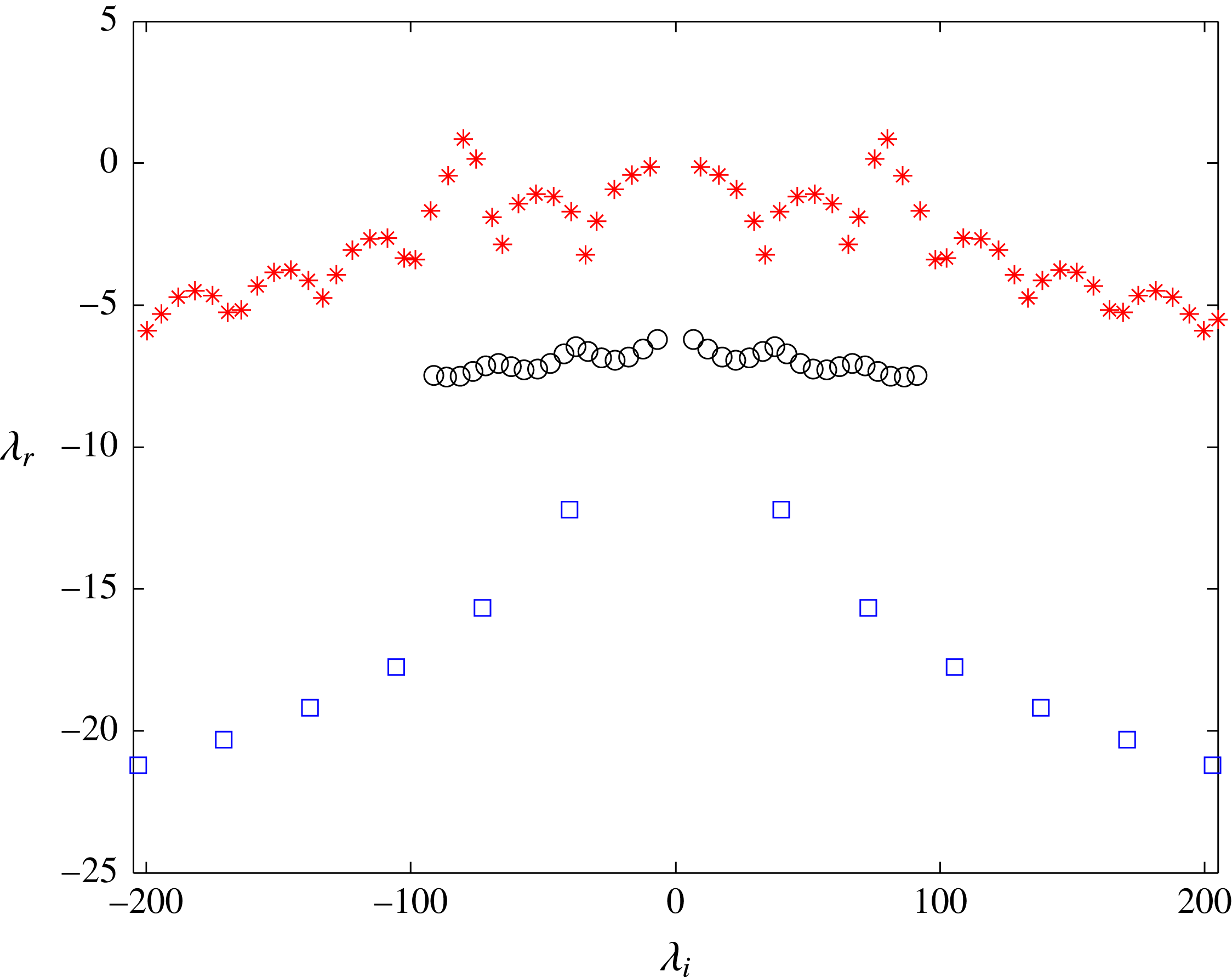
It seems very interesting to compare spectra computed for a relatively high supercritical Weber number, at which the effects of the surface tension begin to be negligible, and for the critical values of
 $We=1.02$
and
 $We=0.98$
, hence just above and below the critical threshold, as illustrated in figure 8. The geometrical configuration of test A of Binnie (Reference Binnie1974) is assumed as the starting condition, for which
 $We=95.9$
,
 ${\mathcal{K}}=5.87\times 10^{3}$
,
 $Fr=7.69$
. Thus, due to the lack of experimental data in the subcritical regime, a virtual numerical experiment has been carried out by starting from the condition of test A of Binnie (Reference Binnie1974) and reducing the liquid flow rate (i.e. velocity) until obtaining
 $We=0.98$
,
 ${\mathcal{K}}=5.75\times 10^{5}$
,
 $Fr=0.076$
. Figure 8 uncovers the characteristic wavy trend of a supercritical regime and shows increasingly stable eigenvalues as the Weber number is reduced. Reducing the liquid flow rate from the value of test A of Binnie (Reference Binnie1974) down to the value of the subcritical regime leads to the frequency variations reported in table 3 for the first five inner modes. For each mode, the frequency is at first reduced until the critical threshold is reached, then it sharply increases below
 $We=1$
, due to the emergence of fast modes in the subcritical regime. Figures 9 and 10 report first, second, third, fifth modes associated with the corresponding inner eigenvalues for
 $We=0.98$
and
 $We=1.02$
, respectively, to be compared with the modes of figure 7 referring to
 $We=95.9$
.
Spectra computed for various conditions of test A of Binnie (Reference Binnie1974).
 $We=95.9$
,
 ${\mathcal{K}}=5.87\times 10^{3}$
,
 $Fr=7.69$
(*);
 $We=1.02$
,
 ${\mathcal{K}}=5.5\times 10^{5}$
,
 $Fr=0.08$
(○);
 $We=0.98$
,
 ${\mathcal{K}}=5.75\times 10^{5}$
,
 $Fr=0.076$
(▫).

First, second, third and fifth eigenmodes for the test A of Binnie (Reference Binnie1974) and for
 $We=1.02$
,
 ${\mathcal{K}}=5.5\times 10^{5}$
,
 $Fr=0.08$
.

First, second, third and fifth eigenmodes for test A of Binnie (Reference Binnie1974) and for
 $We=0.98$
,
 ${\mathcal{K}}=5.75\times 10^{5}$
,
 $Fr=0.076$
.

Computed inner modal frequencies of test A of Binnie (Reference Binnie1974) when reducing the liquid flow rate.

With reference to the first mode only, figure 11 illustrates graphically the sharp increase in the frequency of mode 1 when entering the subcritical regime as the Weber number is reduced. The arrow indicates the frequency route and
 $\unicode[STIX]{x0394}\unicode[STIX]{x1D706}_{i+}$
and
 $\unicode[STIX]{x0394}\unicode[STIX]{x1D706}_{i-}$
represent the frequencies related to the crossing time of the fast and slow waves, respectively, which are analytically evaluated as
 $$\begin{eqnarray}t_{cross\pm }=2Fr\left[\frac{1}{2}\left(U|_{1}-1\right)\mp \frac{1}{\sqrt{We}}\left(\sqrt{U|_{1}}-1\right)+\frac{1}{We}\log \frac{\sqrt{U|_{1}}\pm \displaystyle \frac{1}{\sqrt{We}}}{1\pm \displaystyle \frac{1}{\sqrt{We}}}\right].\end{eqnarray}$$
Frequency route from supercritical to subcritical regime; mode 1;
 $Fr=0.077$
.

The result depicted in figure 11 requires an experimental validation. In addition, it should be used carefully because it refers to the inner first mode, and the present theory is not able to predict the actual selection mechanism of the frequency; hence, future experimental data should be compared with analogous routes referring to higher modes, and a jump from supercritical to subcritical modes of higher order cannot be excluded. Finally, to obtain the expected frequencies, one should multiply
 $\unicode[STIX]{x0394}\unicode[STIX]{x1D706}_{i+}$
and
 $\unicode[STIX]{x0394}\unicode[STIX]{x1D706}_{i-}$
by a factor equal to approximately 1.25 according to the one-plus-one-quarter resonance criterion.
Curves of marginal stability and routes towards the instability. (a) The thick blue lines refer to stable states, the dashed thick red lines to unstable states; the inset represents the dashed rectangular range; the open circle is the condition of test A of Binnie (Reference Binnie1974). (b) Trends for very low
 ${\mathcal{K}}$
values.

Starting again from the condition of test A of Binnie (Reference Binnie1974), and with reference to the first mode only, figure 12(a) depicts two routes towards the instability in the plane
 $Fr-{\mathcal{K}}$
, the vertical one referring to an increase in the chamber width
 $W^{\ast }$
, the hyperbolic one referring to an increase in the flow velocity
 $U_{in}^{\ast }$
. In both cases the thick blue line corresponds to stable states, the dashed thick red line to unstable states. Because of the one-to-one correspondence between physical quantities and dimensionless parameters observed before for the case of water sheet flowing in air, the Weber number of each state is unique (for instance, in the starting point, denoted by the open circle symbol, it is
 $Fr=7.69$
,
 ${\mathcal{K}}=5870$
,
 $We=95.9$
) and the stable/unstable nature of a given status has to be inspected with reference to the neutral stability curve relative to that
 $We$
value. In particular, along the vertical path the
 $We$
number is constant, whilst along the other path
 $We$
increases towards the instability. Such routes are depicted together with various neutral stability curves evaluated for
 $We$
numbers equal to
 $95.9,300.98,10^{4}$
(with this last value closely simulating the case of absence of surface tension). Note that
 $We=95.9$
and
 $We=300.98$
coincide with the stable–unstable marginal values along the two routes here considered. According to a previous finding of De Rosa et al. (Reference De Rosa, Girfoglio and de Luca2014), for each
 $We$
number the unstable region is contained in between two marginal curves, with the lower ones being practically independent of the
 $We$
number, as is better evinced in figure 12(b) illustrating the range of very low
 ${\mathcal{K}}$
values. The asymptotic value of
 ${\mathcal{K}}=19.74$
attained for high
 $Fr$
numbers uncovers the analogous result of De Rosa et al. (Reference De Rosa, Girfoglio and de Luca2014) who neglected the surface tension and defined the Froude number as the reciprocal of the present one. Figure 12(a) clearly shows the stabilizing role of the surface tension, because the unstable region is reduced with decreasing the Weber number. The subcritical regimes are always stable, as predicted by the Frobenius analysis. For the sake of completeness the inset of figure 12(a), corresponding to the dashed rectangle in the main panel, magnifies the range of
 $Fr$
values less than 0.6 and gives an insight as regards the local minima of the upper marginal curves. Data reported in figure 12 have to be used very carefully because the system can exhibit higher modes in different flow conditions.
6 Conclusions
The dynamic behaviour of nappe oscillation has been revisited with reference to a physical model in which a thin liquid sheet interacts with a one-sided closed air chamber. The mutual influence of the air within the enclosure with the compliant nappe interface self-induces a forcing whose features have been investigated. A major motivation for the work is given by the circumstance that, in the presence of surface tension effects, the equation governing the evolution of small disturbances exhibits a singularity at the vertical station where the local flow velocity equals the capillary waves velocity (critical station). The study has been carried out by developing a simplified inviscid, one-dimensional physical model in the context of a linearized formulation of free-interface convection dominated systems.
The modal analysis confirmed the physical argument that any disturbance evolves as the propagation of two wave fronts both directed downstream or one downstream and the other one upstream, depending on whether the flow is supercritical or subcritical, respectively. In this respect the governing equation resembles that featuring the forced vibrations of a string of finite length, formulated in the reference frame moving with the flow velocity. From another perspective, the overall system behaves as a driven damped spring–mass oscillator, where the liquid sheet acts as the mass and the air enclosure as the spring. Thus, the dynamics of the flow system reveals two characteristic frequencies: that of the spring–mass behaviour scaling with the square root of the air chamber equivalent stiffness and that of the capillary waves travelling over the finite length sheet. In every situation the inlet section is considered as a perfectly reflecting boundary. As regards the other boundary condition, in the supercritical regime it is of null centreline slope at the inlet; in the subcritical regime it is imposed at just the singularity station by enforcing the boundedness requirement of the sheet slope there. The behaviour of the solution at the singularity point has also been investigated analytically by employing the Frobenius theory of singular ordinary differential equations.
The results of the modal analysis agree quite strictly with previous experimental data of the literature, available in the supercritical regime only, concerned with sheet deflection and oscillation frequency. A major point is that the spring–mass behaviour natural frequency was never detected in experiments, because high wavenumbers are damped by viscosity, although the related eigenmode is almost always the least stable one. Conversely, observed sheet shapes and measured frequencies are very much in agreement with lower-frequency modes and eigenvalues related to the propagation of waves over the forced vibrating sheet (inner local maxima of spectrum). It is worth noting that for the stable cases the dynamics of nappe oscillation turns out to be a frequency response problem, where the forcing frequency is a self-induced effect which is determined as a part of the solution.
As regards the critical regime of
 $We=O(1)$
, where experimental data for the flat nappe configuration are missing, the major theoretical result is a sharp increase in the oscillation frequency as the flow Weber number is gradually reduced, from supercritical to subcritical values, due to the shift of the prevailing mode from the slow one to the fast one. This conclusion needs of course a careful experimental validation. Marginal stability curves and routes towards the instability are discussed as well.
Supplementary movie
Supplementary movie is available at https://doi.org/10.1017/jfm.2017.241.