


1 Introduction
Frequency lock-in is the synchronization phenomenon between two or more oscillators. The first known report of this fundamental concept dates back to the year 1665, when Christiaan Huygens described the synchronous motion of two pendulum clocks mounted on a wooden beam (Huygens Reference Huygens1893). The same mechanism has been investigated by Lord Rayleigh on coupled tuning forks in his ‘Theory of Sound’ (Rayleigh Reference Rayleigh1907). Later, Van der Pol provided a systematic theoretical treatment of the subject in the context of triode electronic generators. To date, synchronization has accessed standard text books (Pippard Reference Pippard2007; Strogatz Reference Strogatz2012) and is known in many fields of science and engineering. It explains, for example, spontaneous rhythmic applause in theatres (Néda et al. Reference Néda, Ravasz, Vicsek, Brechet and Barabási2000), swarm behaviour of certain animals (Mirollo & Strogatz Reference Mirollo and Strogatz1990), coordinated oscillation of pacemaker cells in the human heart (Torre Reference Torre1976) and orderly motion of galaxies in the universe (Sugimoto & Makino Reference Sugimoto and Makino1989).
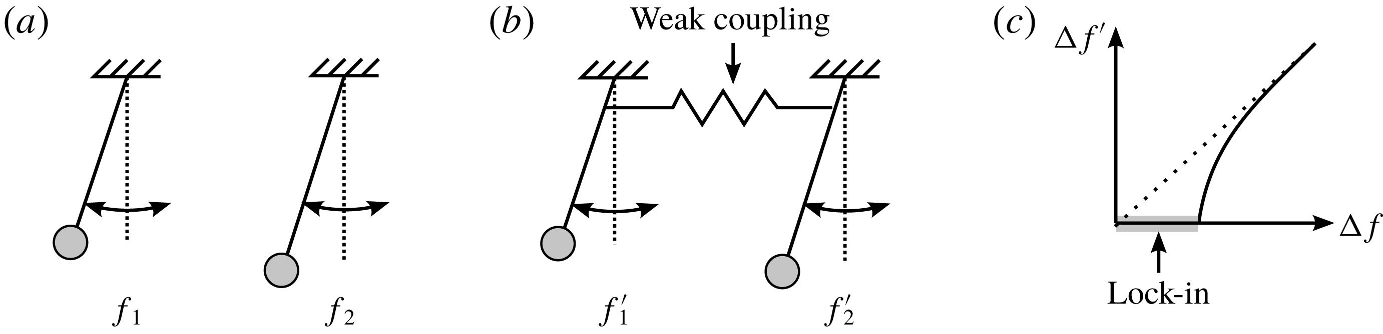
An illustrative example on the working principle is given in figure 1. Two pendulums of different lengths are mounted separately in figure 1(a) and can oscillate unhindered at their natural frequency. This frequency depends on the length of the arm and can be determined by solving an eigenvalue problem of the linearized equation of motion. If both oscillators are coupled, for instance by a spring in figure 1(b), energy can be exchanged and work is done by one oscillator on the other and vice versa. This work yields variations of the amplitudes and hence leads to a new frequency. The same applies to the phase of the pendulums. This mechanism is widely known as lock-in, entrainment or synchronization and is illustrated in figure 1(c). It is also applicable to multiples of the fundamental frequency, meaning that one oscillator can for instance entrain to the higher harmonic of another oscillator (Jenkins Reference Jenkins2013). After disturbing such a system, it will automatically return to a state of synchrony after some time.
(a) Oscillators without coupling, (b) weak coupling and (c) frequency lock-in.
A prominent example of frequency lock-in in fluid mechanics is the vibration of a circular cylinder due to the von Kármán vortex street (Stansby Reference Stansby1976; Ongoren & Rockwell Reference Ongoren and Rockwell1988). Self-induced vortices behind the cylinder can cause vibrations, if the vortex frequency matches to the natural (resonance) frequency of the cylinder, which depends on its mass and elasticity. Although this mechanism can be considered as forced resonance (Jenkins Reference Jenkins2013), the forcing originates from self-induced vortices with a considerable large range of synchronization between the resonance frequency of the cylinder and the vortex shedding frequency (Griffin & Ramberg Reference Griffin and Ramberg1974; Govardhan & Williamson Reference Govardhan and Williamson2000; Gabbai & Benaroya Reference Gabbai and Benaroya2005). Within this range, both resonance and vortex shedding frequencies synchronize (lock-in) to one combined frequency. It has been shown in experiments by Sreenivasan, Strykowski & Olinger (Reference Sreenivasan, Strykowski, Olinger and Ghia1987) and Strykowski & Sreenivasan (Reference Strykowski and Sreenivasan1990) that the vortex shedding behind cylinders is self-sustained. Furthermore, the self-sustained oscillation is the outcome of a supercritical Hopf bifurcation at a diameter-based Reynolds number of approximately 45–50, depending on the literature.
The reason why synchronization has not yet received much attention in the field of boundary-layer theory might be due to the fact that solving the linearized Navier–Stokes operator as an eigenvalue problem in three dimensions is an extraordinarily heavy task even for modern supercomputers (Theofilis Reference Theofilis2011). As a result, there are limited cases where three-dimensional (3-D) flows have been analysed by global linear stability theory (LST). Some of them have been performed by Loiseau et al. (Reference Loiseau, Cherubini, Robinet and Leriche2014) and Bucci et al. (Reference Bucci, Puckert, Andriano, Loiseau, Cherubini, Robinet and Rist2018) for the case of cylindrical roughness elements in the laminar boundary layer. Because synchronization is a nonlinear effect it is not captured by linear theory. Therefore, we provide an experimental investigation on this interesting mechanism in our Laminar Water Channel. The experimental observation will then be compared to the results from 3-D global LST.
The main features of flows perturbed by a 3-D roughness element are vortices, recirculation zones and streaks. One of the most vivid studies on the complex formation of vortices has probably been done by Acarlar & Smith (Reference Acarlar and Smith1987), who visualized both horseshoe vortices in front of the roughness and hairpin vortices emerging from the recirculation zone in the near wake of the roughness. Horseshoe vortices are wrapped around the roughness with their legs extending in the streamwise direction behind the roughness. The aft recirculation zone is surrounded by high wall-normal and spanwise shear and is therefore a region of high sensitivity and the origin of hairpin vortex shedding at high Reynolds numbers (Klebanoff, Cleveland & Tidstrom Reference Klebanoff, Cleveland and Tidstrom1992). Steady streamwise vortices are known to give rise to streaks (Landahl Reference Landahl1990), which dominate the far wake of the roughness and can lead to both destabilization (Loiseau et al. Reference Loiseau, Cherubini, Robinet and Leriche2014) and stabilization of the flow (Fransson et al. Reference Fransson, Brandt, Talamelli and Cossu2005), depending on the set-up and parameters.
Instability modes can be characterized according to their spanwise symmetry, which is either sinuous (antisymmetric) or varicose (symmetric). This distinction is relevant to the present work and is also known from the literature. Without the presence of a roughness, the sinuous mode is usually the first and dominant mode to destabilize boundary-layer streaks (Andersson et al. Reference Andersson, Brandt, Bottaro and Henningson2001; Schlatter et al. Reference Schlatter, Brandt, Lange and Henningson2008; Vaughan & Zaki Reference Vaughan and Zaki2011). This is not always the case when roughness-induced streaks are investigated. Cherubini et al. (Reference Cherubini, De Tullio, De Palma and Pascazio2013) discovered large energy gain of varicose perturbations when the boundary layer is perturbed by a three-dimensional roughness hump. This result was confirmed for a hemispherical roughness element by Citro et al. (Reference Citro, Giannetti, Luchini and Auteri2015) and is also in agreement with the experimental observation of symmetric hairpin vortices emerging from the recirculation zone of the roughness (Ye, Schrijer & Scarano Reference Ye, Schrijer and Scarano2018). Varicose modes are mainly driven by wall-normal shear in regions of low streamwise velocity and related to Kelvin–Helmholtz instabilities, whereas sinuous modes are driven by spanwise shear that may lead to a meandering motion similar to the von Kármán vortex streak behind blunt bodies.
To understand the mode symmetry better, Loiseau et al. (Reference Loiseau, Cherubini, Robinet and Leriche2014) performed a global linear stability analysis on cylindrical roughness elements of different aspect ratios
 $\unicode[STIX]{x1D702}=d/k$
, where
 $d$
is the diameter and
 $k$
the height of the roughness. These authors found that the leading global mode is sinuous if
 $\unicode[STIX]{x1D702}$
is small, e.g. at or below unity. For larger aspect ratios, the leading mode is varicose for both globally stable and unstable modes. This is in agreement with the experimental investigation by Asai, Minagawa & Nishioka (Reference Asai, Minagawa and Nishioka2002), where the varicose mode was highly sensitive to the width of the low-speed streak. In global linear stability analyses, the critical Reynolds number is the threshold where the system becomes globally unstable. Note that this term has been used to describe transition in many earlier studies (von Doenhoff & Braslow Reference von Doenhoff and Braslow1961; Tani et al.
Reference Tani, Komoda, Komatsu and Iuchi1962; Klebanoff et al.
Reference Klebanoff, Cleveland and Tidstrom1992) and its meaning may thus be confusing. In the present work, we distinguish between the critical Reynolds number (3-D global instability) and the transition (tripping to turbulence) Reynolds number. Puckert & Rist (Reference Puckert and Rist2018a
) showed that the critical Reynolds number from 3-D global LST is typically larger than the transition Reynolds number. Bucci et al. (Reference Bucci, Puckert, Andriano, Loiseau, Cherubini, Robinet and Rist2018) explained the subcritical instability in the experiment as a result of quasi-resonance of a varicose, stable global mode. In contrast to convective instabilities, a global instability is intrinsic and does not depend on external periodic forcing (Huerre & Monkewitz Reference Huerre and Monkewitz1990; Theofilis Reference Theofilis2003; Chomaz Reference Chomaz2005).
In the present work, the set-up of Bucci et al. (Reference Bucci, Puckert, Andriano, Loiseau, Cherubini, Robinet and Rist2018) and Puckert & Rist (Reference Puckert and Rist2018a ) is reproduced to investigate the nonlinear interaction between sinuous and varicose modes and to suggest synchronization as an important nonlinear mechanism in boundary layers.
The questions to be answered in this study are:
(i) Are the sinuous and varicose modes nonlinearly coupled?
(ii) Can the frequency of sinuous and varicose modes synchronize (lock-in)?
(iii) What does the physical flow look like?
(iv) What is the role of the critical Reynolds number in this context?
This paper is structured in four sections: first, the experimental set-up is described in § 2. Hot-film measurements are presented in § 3 to investigate the spectral behaviour of the roughness wake. Particle image velocimetry (PIV) is then performed in § 4 to provide details on the observed frequency lock-in. In the end, conclusions are given in § 5.
2 Experimental set-up
For the present investigations, the Laminar Water Channel (Laminarwasserkanal, LaWaKa) at the Institute of Aerodynamics and Gas Dynamics (IAG) at the University of Stuttgart is used. It is a closed-loop facility with a turbulence intensity of 0.05 % of the free-stream velocity in a frequency range of 0.1–10 Hz at
 $0.145~\text{ms}^{-1}$
(Wiegand Reference Wiegand1996). The dimensions of the test section are
 $10\times 1.2\times 0.2~\text{m}^{3}$
and a flat plate is installed in the test section to create a two-dimensional (2-D) laminar boundary layer of Blasius type. Boundary-layer thickening in the corners of the test section is reduced by suction through a small gap between the flat plate and the side walls. More details on the flow facility and the fluctuation levels inside the boundary layer can be found in Wiegand (Reference Wiegand1996) and Puckert & Rist (Reference Puckert and Rist2018a
).
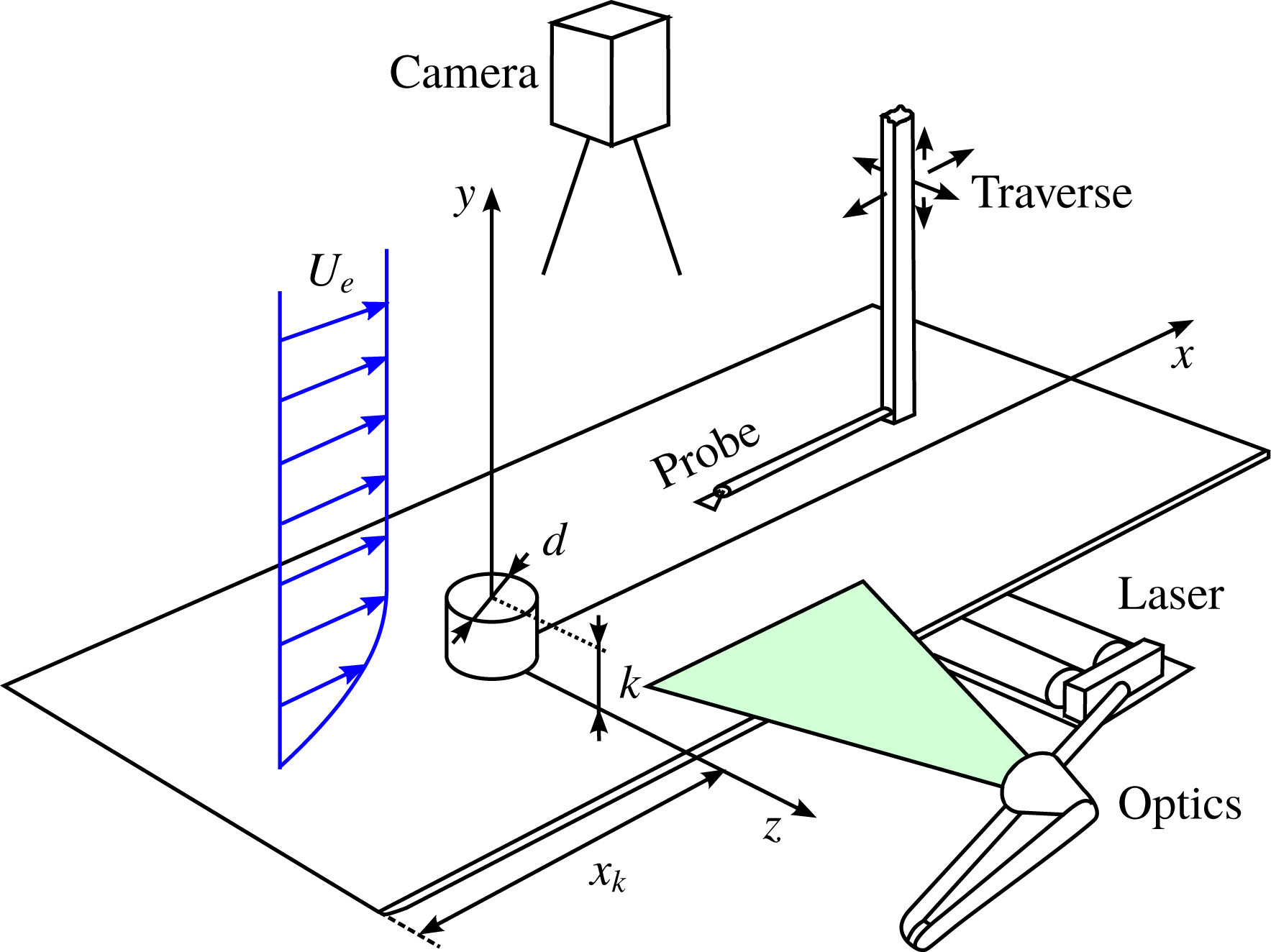
The roughness set-up is sketched in figure 2. A cylindrical, isolated roughness element with constant height
 $k=0.01~\text{m}$
is located at the spanwise centre of the flat plate at a station
 $x_{k}$
from the leading edge of the flat plate. The bottom of the roughness is the origin of the non-dimensional coordinate system, with
 $x$
-,
 $y$
- and
 $z$
-coordinates extending in the streamwise, wall-normal and spanwise directions, respectively. All length scales in this work are non-dimensionalized by
 $k$
. The control parameter is the Reynolds number
 $Re_{k}=kU_{e}/\unicode[STIX]{x1D708}$
with boundary-layer edge velocity
 $U_{e}$
and kinematic viscosity
 $\unicode[STIX]{x1D708}$
. In the present experiments,
 $Re_{k}$
is controlled by changing
 $U_{e}$
, while
 $k$
and
 $\unicode[STIX]{x1D708}$
remain constant. The frequencies in this work are also presented non-dimensionally as circular frequency
 $\unicode[STIX]{x1D714}=2\unicode[STIX]{x03C0}f\,kU_{e}^{-1}$
, where
 $f$
is the physical frequency in Hertz. This notation is advantageous to compare with the works of Loiseau et al. (Reference Loiseau, Cherubini, Robinet and Leriche2014) and Bucci et al. (Reference Bucci, Puckert, Andriano, Loiseau, Cherubini, Robinet and Rist2018), where the circular frequency is a result of 3-D global linear stability analyses.
Experimental set-up.
In this study, three roughness elements are used: one with aspect ratio
 $\unicode[STIX]{x1D702}=3$
and two with
 $\unicode[STIX]{x1D702}=1$
. Recall from the previous section that the aspect ratio is the diameter
 $d$
of the cylindrical roughness divided by the roughness height
 $k$
. The choice of
 $\unicode[STIX]{x1D702}$
allows for an evaluation of three important configurations which are already known from the 3-D global linear stability analyses of Loiseau et al. (Reference Loiseau, Cherubini, Robinet and Leriche2014) and Bucci et al. (Reference Bucci, Puckert, Andriano, Loiseau, Cherubini, Robinet and Rist2018). Parameter studies on the aspect ratio have already been done by Loiseau et al. (Reference Loiseau, Cherubini, Robinet and Leriche2014) and Puckert & Rist (Reference Puckert and Rist2018a
). As discussed in the introduction, the first unstable global mode is sinuous for configurations with small aspect ratios (of the order of
 $\unicode[STIX]{x1D702}\leqslant 1$
) and varicose instabilities for configurations with large aspect ratios (of the order of
 $\unicode[STIX]{x1D702}\geqslant 3$
). Both cases are thus considered in the present work.
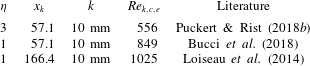
Detailed parameters and references to the literature are listed in table 1. The parameter space of the hot-film measurements for the configuration
 $\unicode[STIX]{x1D702}=3$
are 31 Reynolds numbers in the range
 $370<Re_{k}<804$
at 19 stations between
 $2<x<40$
. For the configuration
 $(\unicode[STIX]{x1D702},x_{k})=(1,57.1)$
, 26 Reynolds numbers are used between
 $578<Re_{k}<952$
at 20 stations between
 $2<x<41$
. The configuration
 $(\unicode[STIX]{x1D702},x_{k})=(1,166.4)$
is only investigated with PIV in this work.
Parameters of the three configurations considered in this study.
 $Re_{k,c,e}$
is the critical Reynolds number from experimental observations.
The hot-film system consists of a Dantec Streamware frame with a Wheatstone bridge in constant-temperature anemometry (CTA) mode and a Dantec 55R15 boundary-layer probe with overheat ratio 8 %. Voltage signals are acquired by a 16 bit A/D converter and recorded on a computer with automated LabVIEW programs. A computer-controlled traverse system moves the probe to various positions in the test section. The calibration of the hot-film is done in situ by traversing the probe through resting water to obtain calibration coefficients for King’s law. The voltage signals from the experiment are then transferred to physical velocity signals. Due to the low frequencies in the water channel compared to low-speed wind tunnels, a sampling rate of 100 Hz is sufficiently large to acquire signals at a good temporal resolution (Wiegand Reference Wiegand1996).
The PIV system is operated with a double-pulsed Nd:YAG laser (Quantel Brilliant Twins) with a pulse rate of 10 Hz. The laser is guided through an optical apparatus and forms a laser light sheet parallel to the flat plate at the height of the roughness (
 $y=1$
). The laser sheet illuminates polyamide tracer particles of
 $4.2~\unicode[STIX]{x03BC}\text{m}$
diameter which are recorded by a 12-bit PCO SensiCam camera. The camera is mounted perpendicular to the illuminated laser sheet at a distance of 0.7 m. Cross-correlation of the double images provides time-resolved vector fields of the flow in the
 $xz$
plane. More details on both hot-film anemometry and PIV are described in Puckert (Reference Puckert2019).
3 Roughness-induced instabilities
The first task in this section is to find a suitable measurement position for the hot-film probe. Once this is known, the transition and critical Reynolds numbers are determined. Time traces from hot-film signals are then analysed to characterize the type of roughness-induced instabilities. This preliminary work is necessary to recognize the connection between frequency lock-in and global instability. Frequency spectra at various Reynolds numbers are then investigated and compared to theory. At the end of the section, evidence for synchronization is discussed.
3.1 Downstream disturbance evolution
The evolution of the streamwise disturbance velocity is investigated in figure 3 to identify the streamwise position for more detailed hot-film measurements and to determine the transition Reynolds number. The position of the probe is
 $(y,z)=(1,0)$
, which is close to the highest wall-normal shear (Puckert & Rist Reference Puckert and Rist2018a
). Figure 3 shows the root mean square of velocity fluctuations
 $u_{rms}^{\prime }/U_{e}$
with respect to time at different stations
 $x$
and Reynolds numbers
 $Re_{k}$
for two configurations: (a)
 $\unicode[STIX]{x1D702}=3$
and (b)
 $(\unicode[STIX]{x1D702},x_{k})=(1,57.1)$
. The non-dimensionalization is done with the boundary-layer edge velocity
 $U_{e}$
of the undisturbed flow. Here,
 $U_{e}$
can be assumed steady, thus comparable to the base flow from numerical simulations. Since the most interesting results in this section are the different aspect ratios, the configuration
 $(\unicode[STIX]{x1D702},x_{k})=(1,166.4)$
is omitted.
Streamwise evolution of velocity disturbances at
 $(y,z)=(1,0)$
for (a)
 $\unicode[STIX]{x1D702}=3$
and (b)
 $(\unicode[STIX]{x1D702},x_{k})=(1,57.1)$
at different
 $Re_{k}$
as indicated in legend.

In both figure 3(a,b), the disturbance level rapidly rises between the roughness rear end and
 $x\approx 6$
. Further downstream, the disturbance level changes only gradually or remains constant at approximately
 $u_{rms}^{\prime }/U_{e}=10^{-1}$
, depending on the Reynolds number. For low Reynolds numbers, the fluctuation level is considerably lower and tends to fluctuate more. It is reasonable to assume that this difference is due to a laminar versus turbulent flow. The laminar-to-turbulent transition thus happens in the range
 $429<Re_{k}<517$
in figure 3(a) and in the range
 $632<Re_{k}<712$
in figure 3(b). Comparing these results to the literature is interesting. For instance, Fransson et al. (Reference Fransson, Brandt, Talamelli and Cossu2005) found transition in a wind tunnel for the same set-up as in figure 3(a) at
 $Re_{k}=502$
. This is in good agreement with the present transition range for the configuration
 $\unicode[STIX]{x1D702}=3$
, validating our assumption. The disturbance level near
 $u_{rms}^{\prime }/U_{e}=10^{-1}$
represents the turbulent state. In figure 3(b), laminar-to-turbulent transition is even more pronounced than in figure 3(a).
It can be inferred from figure 3 that the decision whether or not the flow becomes turbulent is made close to the roughness. Cases with a high disturbance level of approximately
 $u_{rms}^{\prime }/U_{e}=10^{-1}$
become turbulent further downstream. The high disturbance level close to the roughness is a result of vortex shedding in the near wake of the roughness (Acarlar & Smith Reference Acarlar and Smith1987). By performing 2-D LST, Siconolfi, Camarri & Fransson (Reference Siconolfi, Camarri and Fransson2015) found that the near wake is a region of strong bi-local instability. Furthermore, Loiseau et al. (Reference Loiseau, Cherubini, Robinet and Leriche2014) used the product of direct and adjoint 3-D global modes to find the region of possible inception of the global mode (‘wavemaker’ region). These authors identified a possible wavemaker in the near wake at the height of the roughness. Both our preliminary experiment and theory agree that the near wake is a location of great significance. Therefore, the hot-film probe in the following investigations is placed at
 $x=6$
for the configurations
 $\unicode[STIX]{x1D702}=3$
and at
 $x=5$
for
 $(\unicode[STIX]{x1D702},x_{k})=(1,57.1)$
. The wall-normal position is set to
 $y=1$
, where Puckert & Rist (Reference Puckert and Rist2018b
) found the maximum disturbance amplitude in wall-normal direction behind the roughness. Note that the experimental disturbances in this study are nonlinear whereas the analysis of Loiseau et al. (Reference Loiseau, Cherubini, Robinet and Leriche2014) is based on the linearization of the underlying equations.
Time traces in seconds for (a)
 $\unicode[STIX]{x1D702}=3$
at
 $x=6$
and (b)
 $(\unicode[STIX]{x1D702},x_{k})=(1,57.1)$
at
 $x=5$
with different
 $Re_{k}$
as indicated on the ordinate axes. Same non-dimensional amplitude scaling and spacing
 $0.4U_{e}$
for all time traces.

A more detailed analysis is done at this position to find the critical Reynolds number. Following the work of Puckert & Rist (Reference Puckert and Rist2018b
), non-dimensional time traces
 $u^{\prime }/U_{e}$
are presented for different Reynolds numbers in figure 4(a,b) for the configurations
 $\unicode[STIX]{x1D702}=3$
and
 $(\unicode[STIX]{x1D702},x_{k})=(1,57.1)$
, respectively. Note that the time traces appear slightly compressed with increasing Reynolds number due to non-dimensionalization. As expected, the time traces reveal periodic fluctuations. In figure 4(a), the non-dimensional fluctuation amplitude becomes initially stronger and remains at a constant value when exceeding a Reynolds number in the range of
 $541<Re_{k}<574$
. Furthermore, the frequency continuously increases when increasing the Reynolds number. The same observations can be made in figure 4(b). In this configuration, the frequency changes rapidly between
 $833<Re_{k}<865$
and the fluctuation amplitude becomes lower thereafter. This changeover from low-frequency to high-frequency oscillation is triggered by a nonlinear mechanism. Based on these observations, Puckert & Rist (Reference Puckert and Rist2018a
) introduced the experimental critical Reynolds number,
 $Re_{k,c,e}$
, which is the experimental counterpart to the theoretical critical Reynolds number,
 $Re_{k,c,t}$
, from 3-D global LST. A more detailed study yields
 $Re_{k,c,e}=556$
for the configuration
 $\unicode[STIX]{x1D702}=3$
in the same non-dimensional set-up (Puckert & Rist Reference Puckert and Rist2018b
). The agreement with the critical Reynolds number from theory was reported to be within 1 % error. For the configuration
 $(\unicode[STIX]{x1D702},x_{k})=(1,57.1)$
, the experimental critical Reynolds number can be interpolated linearly between 833 and 865 and thus yields
 $Re_{k,c,e}=849$
. For this configuration, no critical Reynolds number has been published yet, but Bucci et al. (Reference Bucci, Puckert, Andriano, Loiseau, Cherubini, Robinet and Rist2018) provides a range for this configuration of
 $700<Re_{k,c,t}<900$
. This confirms that
 $Re_{k,c,e}=849$
is a reliable threshold with respect to 3-D global instability. For the configuration
 $(\unicode[STIX]{x1D702},x_{k})=(1,166.4)$
, the critical Reynolds number has already been determined by Puckert & Rist (Reference Puckert and Rist2018a
) and is
 $Re_{k,c,e}=1025$
. Later, the critical Reynolds number will turn out to be an important threshold for synchronization. For convenience, all results are summarized in table 1.
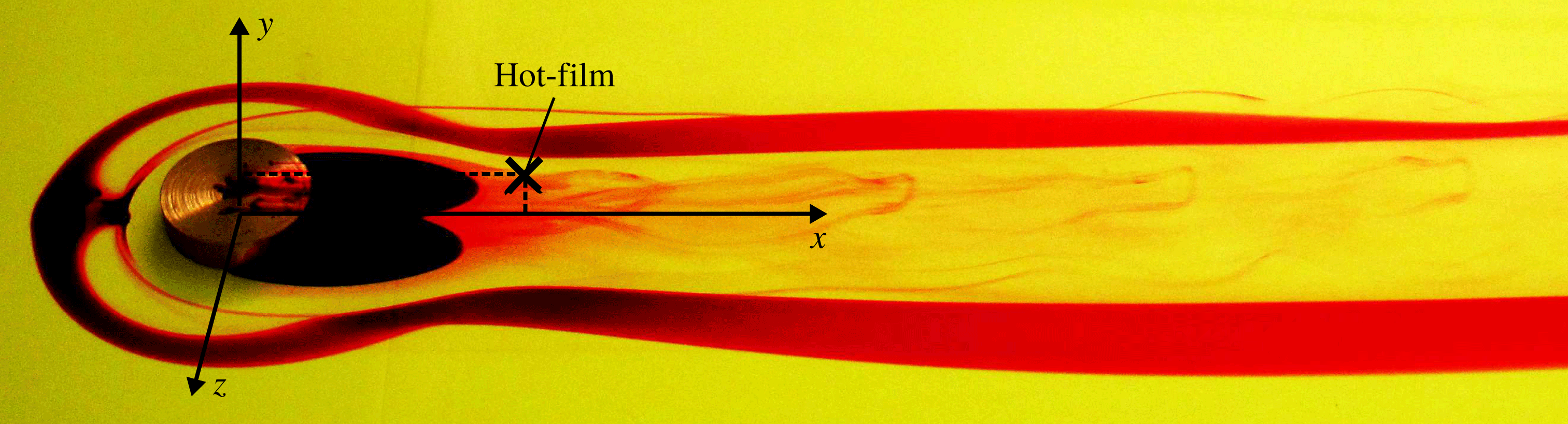
One of the great advantages of water channels is the visualizations. Figure 5 shows a snapshot of the configuration
 $\unicode[STIX]{x1D702}=3$
visualized with potassium permanganate at
 $Re_{k}=500$
. Dye streaklines draw contours of the horseshoe vortex in front of and around the roughness. Dark regions in the roughness wake are footprints of the recirculation zone. Strong hairpin vortex shedding can be seen when looking closely at the vortex filaments. The position of the hot-film probe is indicated by a solid cross. Note that the roughness is additionally disturbed by the potassium permanganate crystals in this picture and the vortex shedding may thus be stronger than without the crystals. The purpose of this figure is to provide the reader a visual impression of the situation.
Visualization with potassium permanganate of the configuration
 $\unicode[STIX]{x1D702}=3$
at
 $Re_{k}=500$
. Flow from left to right.
3.2 Frequency behaviour
In order to investigate the frequency behaviour of the flow, disturbance velocities are transferred to Fourier space via discrete Fourier transforms. Figure 6 provides frequency spectra of the configuration
 $\unicode[STIX]{x1D702}=3$
at two Reynolds numbers: (a)
 $Re_{k}=489$
in the subcritical regime and (b)
 $Re_{k}=602$
in the supercritical regime. In figure 6(a), the power spectral density (PSD) is large in the range
 $0.5<\unicode[STIX]{x1D714}<1$
and at very low frequencies (
 $\unicode[STIX]{x1D714}\rightarrow 0$
). The latter is known to originate from facility-dependent effects at low free-stream velocities (Puckert, Dieterle & Rist Reference Puckert, Dieterle and Rist2017) and will thus be omitted in the analysis. When comparing the remaining spectra of figure 6(a) to figure 6(b), it can be seen that in the latter, a distinctive frequency peak forms at
 $\unicode[STIX]{x1D714}=0.91$
. Puckert & Rist (Reference Puckert and Rist2018b
) explain the changeover from broadbanded to sharp peak with the changeover from convective to global instability. It should be noted that the set-up in this work has the same non-dimensional parameters as in Puckert & Rist (Reference Puckert and Rist2018b
) but a different dimensional roughness size. It is therefore an independent confirmation of the good repeatability of the experimental detection of the critical Reynolds number. What is more important in this paper is the fact that the frequency of the highest PSD does not change significantly when exceeding the critical Reynolds number. This is an important result, because the configuration
 $\unicode[STIX]{x1D702}=1$
is fundamentally different, as will be shown next.
Fourier spectra for
 $\unicode[STIX]{x1D702}=3$
at
 $x=6$
with (a)
 $Re_{k}=489$
and (b)
 $Re_{k}=602$
.
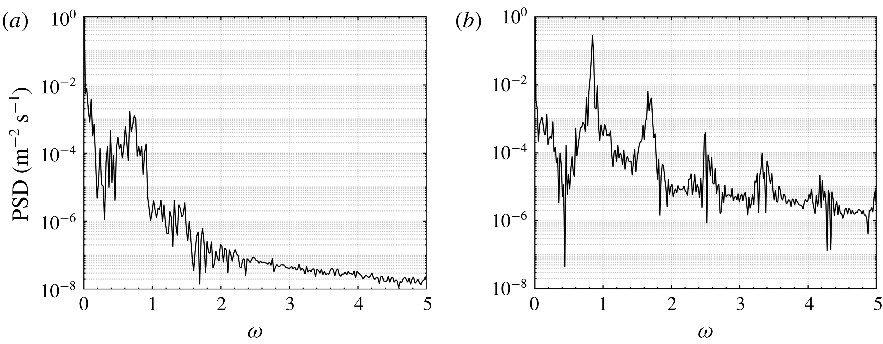
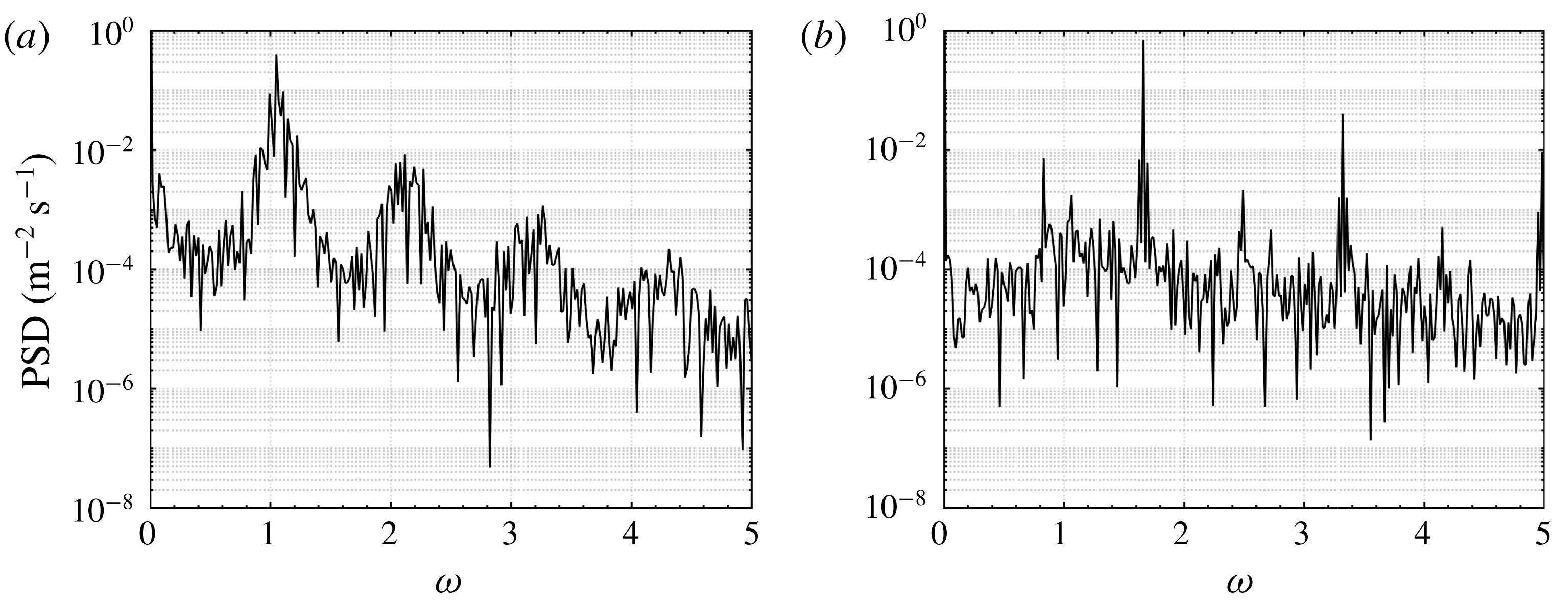
Figure 7(a,b) shows the frequency spectra for
 $(\unicode[STIX]{x1D702},x_{k})=(1,57.1)$
at
 $Re_{k}=805$
and 925, respectively. The dominant frequency in figure 7(a) is at
 $\unicode[STIX]{x1D714}=1.02$
and is much more pronounced than the peak in figure 6(a). From the discussion of the previous configuration, we would expect a spectral peak at a similar frequency when increasing the Reynolds number. However, this expectation is not fulfilled. Figure 7(b) illustrates a dominant, narrow-banded peak at
 $\unicode[STIX]{x1D714}=1.62$
and another peak at
 $\unicode[STIX]{x1D714}=0.81$
. This observation raises three questions: Is this changeover discontinuous or rather gradual? If discontinuous, does it collapse with the critical Reynolds number? What is the connection between the two frequency peaks in figure 7(b)?
Fourier spectra for
 $(\unicode[STIX]{x1D702},x_{k})=(1,57.1)$
at
 $x=5$
with (a)
 $Re_{k}=805$
and (b)
 $Re_{k}=925$
.
To clarify the first two questions, the evolution of the frequency is analysed versus Reynolds number. Figure 8(a) illustrates the frequency of maximum PSD (‘peak frequency’) for the configuration
 $\unicode[STIX]{x1D702}=3$
. The peak frequency continuously grows when
 $Re_{k}$
is increased and is not notably altered beyond the critical Reynolds number at the dashed vertical line. The only change in the supercritical regime is that the points in figure 8(a) have less spread. This can readily be explained by the fact that the frequency peaks of a global instability are more narrow-banded and can be detected with higher experimental precision.
Dominant (‘peak’) frequency versus Reynolds number for (a)
 $\unicode[STIX]{x1D702}=3$
,
 $x=6$
and (b)
 $(\unicode[STIX]{x1D702},x_{k})=(1,57.1)$
,
 $x=5$
; o-shaped markers represent overall maximum, x-shaped markers indicate maximum below
 $\unicode[STIX]{x1D714}=1.2$
.
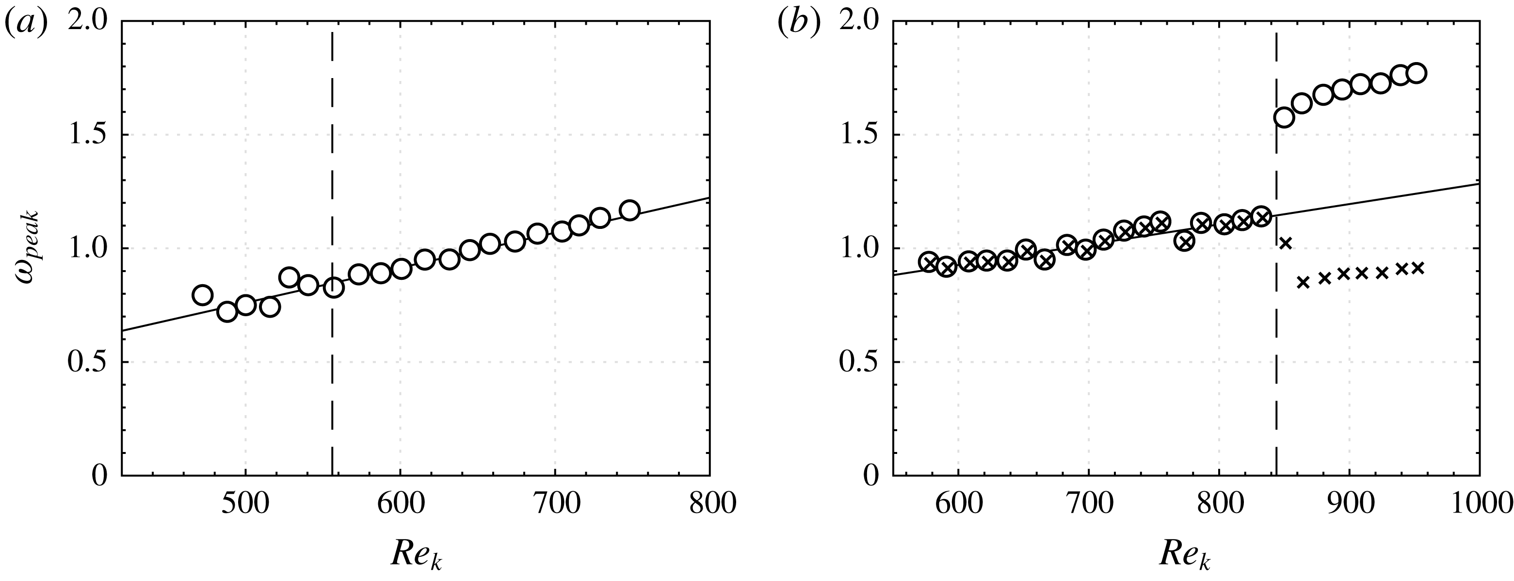
A trend line is added to figure 8(a) to indicate that the growth of the dominant frequency is nearly proportional to the Reynolds number. Recalling the definitions
 $\unicode[STIX]{x1D714}=2\unicode[STIX]{x03C0}fk/U_{e}$
and
 $Re_{k}=U_{e}k/\unicode[STIX]{x1D708}$
, figure 8(a) suggests a linear relation of the physical frequency and square velocity:
 $$\begin{eqnarray}f\propto U_{e}^{2}.\end{eqnarray}$$
This result is in agreement with the experiments by Klebanoff et al. (Reference Klebanoff, Cleveland and Tidstrom1992), who investigated the Strouhal behaviour of hemispherical roughness elements in a laminar boundary layer.
The same analysis is done for the configuration
 $(\unicode[STIX]{x1D702},x_{k})=(1,57.1)$
in figure 8(b). In the subcritical regime, up to the critical Reynolds number, the Strouhal behaviour is very similar to figure 8(a) and equation (3.1). However, something unexpected happens at the critical Reynolds number: the peak frequency suddenly ‘jumps’ to a new level and continues to grow from this new level. An additional set of data has been added to figure 8(b) with ‘x’-shaped markers to include the second peak at the lower frequency. This peak has already appeared in figure 7(b). Clearly, the low-frequency peak follows the same trend as the high-frequency peak (‘o’-shaped markers). In contrast to the subcritical regime, it is difficult to judge whether equation (3.1) is still applicable based on the available measurement points. More importantly, however, it is shown that the changeover of the Strouhal behaviour is discontinuous and that this changeover collapses with the critical Reynolds number.
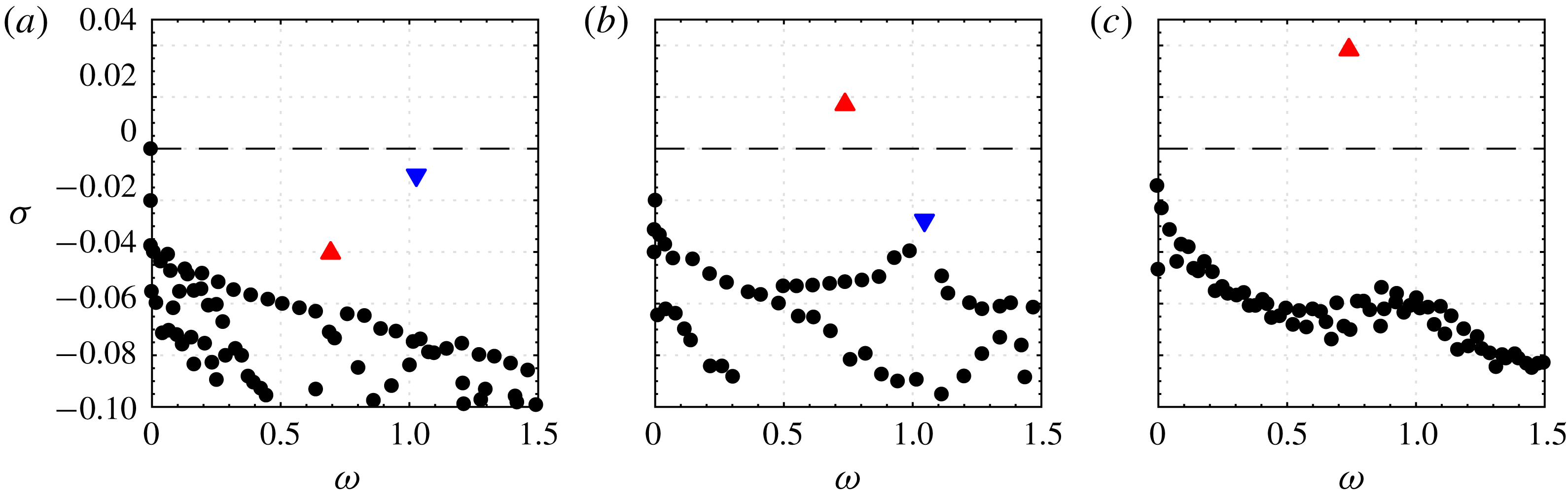
A comparison to theory will substantiate this conclusion. Figure 9 is a reproduction of the eigenvalue spectra from 3-D global LST for the configuration
 $(\unicode[STIX]{x1D702},x_{k})=(1,57.1)$
at
 $Re_{k}=700$
, 900 and 1200 from Bucci et al. (Reference Bucci, Puckert, Andriano, Loiseau, Cherubini, Robinet and Rist2018). The axes measure the frequency
 $\unicode[STIX]{x1D714}$
and the growth rate
 $\unicode[STIX]{x1D70E}$
of the global modes, respectively. The solid black circles represent a branch of stable varicose eigenmodes. Triangles facing up represent isolated sinuous modes and triangles facing down represent isolated varicose modes. For
 $Re_{k}=700$
in figure 9(a), all growth rates of the eigenmodes are negative, indicating global stability. In figure 9(b), the isolated sinuous mode becomes unstable and remains unstable up to large Reynolds numbers, see figure 9(c). These spectra suggest that the theoretical critical Reynolds number is situated in the range
 $700<Re_{k,c,t}<900$
. This range is in agreement with the experimental critical Reynolds number
 $Re_{k,c,e}=849$
determined in § 3.1. A comparison of the leading frequency
 $\unicode[STIX]{x1D714}=1.02$
in figure 9(a) with the peak frequency
 $\unicode[STIX]{x1D714}=0.98$
of figure 8(b) at
 $Re_{k}=700$
yields good agreement. This means that the experimental peak frequency correlates to the varicose global mode. Bucci et al. (Reference Bucci, Puckert, Andriano, Loiseau, Cherubini, Robinet and Rist2018) made a similar observation and concluded that the varicose mode in figure 9(a) can quasi-resonate and become convectively unstable in the experiment.
In figure 9(b), the situation is different. Here, the varicose mode sinks down to the stable part of the diagram and even vanishes in figure 9(c). In contrast, the sinuous mode rises to the unstable part of the diagram and becomes the new leading mode. Interestingly, this changeover has also been observed in the experiment. It is hypothesized that the frequencies marked with ‘x’ in figure 8 correlate with the sinuous global modes in figure 9(b,c). In a direct comparison, the sinuous mode in figure 9(b) at
 $\unicode[STIX]{x1D714}=0.75$
is close to
 $\unicode[STIX]{x1D714}_{peak}=0.89$
in figure 8(b). Although the agreement is not perfect, it could explain the experimental observations. Deviations in the experiment are particularly due to the single position of the hot-film probe. In § 4, this drawback is eliminated by using PIV. It will further be shown that the two peak frequencies in figure 8(b) are indeed sinuous and varicose.
Reproduction of eigenspectrum analyses of
 $(\unicode[STIX]{x1D702},x_{k})=(1,57.1)$
by Bucci et al. (Reference Bucci, Puckert, Andriano, Loiseau, Cherubini, Robinet and Rist2018) for (a)
 $Re_{k}=700$
, (b)
 $Re_{k}=900$
and (c)
 $Re_{k}=1200$
.
At this point, there is enough evidence to suspect synchronization of two modes in the supercritical regime of
 $(\unicode[STIX]{x1D702},x_{k})=(1,57.1)$
. As is known from Bucci et al. (Reference Bucci, Puckert, Andriano, Loiseau, Cherubini, Robinet and Rist2018), the leading varicose mode in this configuration is only stable in the framework of LST. The pseudo-spectral analyses of Bucci et al. (Reference Bucci, Puckert, Andriano, Loiseau, Cherubini, Robinet and Rist2018) reveal that the stable varicose mode can quasi-resonate in a slightly disturbed environment. Since experiments are always disturbed by background noise, stable global eigenmodes can be convectively unstable in physical flows. This manifests itself as a varicose instability associated with hairpin vortex shedding in the subcritical regime. The frequency of this convective instability has been determined in figure 7(b). If an isolated global instability is then added to such a flow, for example by increasing
 $Re_{k}$
beyond the critical Reynolds number, the system needs to adjust itself to the new situation. One possibility is that the stronger global mode could suppress the weaker convective mode. This is unlikely, because the convective mode is strong enough to reach nonlinear saturation in significant parts of the total signal length as shown in figure 4. Another, more likely, possibility is the co-existence of both modes by nonlinear coupling. Regarding the spectrum in figure 7(b) and the close agreement with theory, the synchronized co-existence of both sinuous and varicose modes is the most plausible explanation for the ‘jump’ of the dominant frequency in figure 8(b). The remaining piece of the puzzle is a confirmation that the two frequency peaks in figure 8(b) indeed belong to the sinuous and varicose modes predicted by theory. To do so, PIV is performed as a whole-field method in the following section.
4 Synchronization of sinuous and varicose modes
To confirm the discussion above and to show that the leading modes in the experiment have a sinuous and varicose shape, PIV is used to acquire time-resolved 2-D snapshots at the height of the roughness. These snapshots are analysed with a Fourier mode decomposition. For an introduction into this method the reader is referred to Ma et al. (Reference Ma, Feng, Pan, Gao and Wang2015). Spectra and Fourier modes are investigated for
 $\unicode[STIX]{x1D702}=1$
at
 $Re_{k}=766$
(subcritical) and
 $Re_{k}=930$
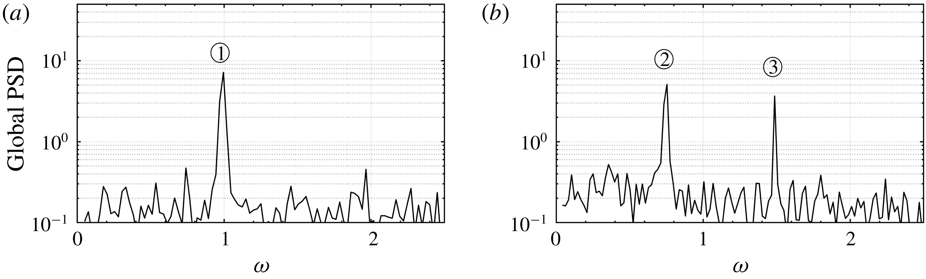
(supercritical), respectively. Figure 10 shows the global power spectra from the Frobenius norm of the PSD for both cases. The global PSD can be imagined as the geometric sum of local spectra at each PIV interrogation window.
Global power spectral density from Fourier decomposition for
 $(\unicode[STIX]{x1D702},x_{k})=(1,57.1)$
at (a)
 $Re_{k}=766$
(subcritical) and (b)
 $Re_{k}=930$
(supercritical).
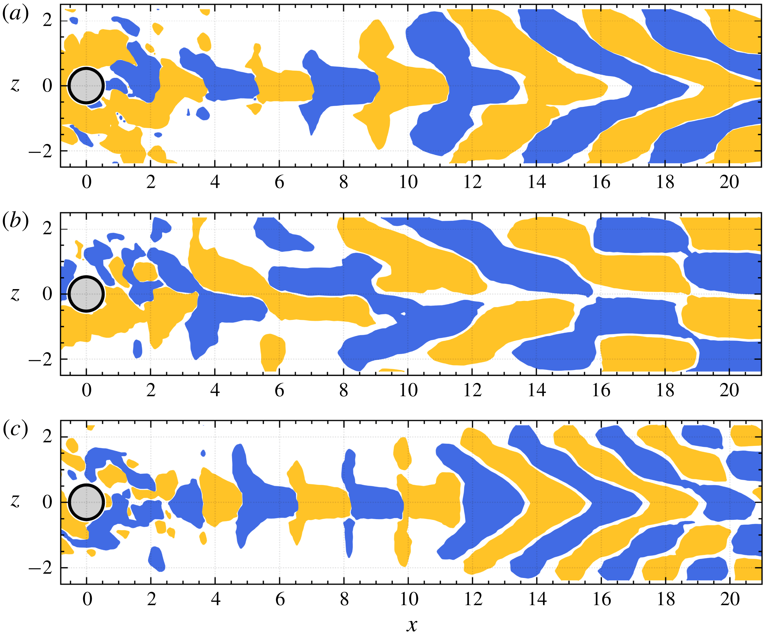
Fourier mode of
 $\pm 0.1$
of maximum streamwise perturbation at (a)
 $\unicode[STIX]{x1D714}=1.0$
(b)
 $\unicode[STIX]{x1D714}=0.74$
and (c)
 $\unicode[STIX]{x1D714}=1.49$
, see figure 10 numbers
 $\unicode[STIX]{x2460}$
,
 $\unicode[STIX]{x2461}$
and
 $\unicode[STIX]{x2462}$
.
The global power spectrum for
 $Re_{k}=766$
in figure 10(a) exhibits a frequency peak at
 $\unicode[STIX]{x1D714}=1.0$
. This is in excellent agreement with the leading frequency from theory (figure 9(a)) and also in line with the hot-film measurements in figure 7(a) and figure 8(b). The supercritical case
 $Re_{k}=930$
in figure 10(b) exhibits two dominant frequencies in the global power spectrum, namely at
 $\unicode[STIX]{x1D714}=0.74$
and
 $\unicode[STIX]{x1D714}=1.49$
. The peak at
 $\unicode[STIX]{x1D714}=0.74$
is again in excellent agreement with the sinuous mode predicted by theory in figure 9(b). This result is an improvement to the hot-film results in figure 8(b). It is known from Loiseau et al. (Reference Loiseau, Cherubini, Robinet and Leriche2014) that the sinuous mode develops further downstream than the varicose mode. In contrast to hot-film anemometry, PIV and 3-D global LST include the streamwise direction and are therefore more representative for the global dynamics of the flow.
Figure 11 exhibits the symmetry shape (sinuous or varicose) of the two frequency peaks in figure 10(b) by illustrating the real part of the decomposition of the streamwise velocity perturbations for the Reynolds numbers
 $Re_{k}=766$
and
 $Re_{k}=930$
. Figure 11(a–c) refers to the numbers
 $\unicode[STIX]{x2460}$
,
 $\unicode[STIX]{x2461}$
and
 $\unicode[STIX]{x2462}$
in figure 11, respectively. It shows the Fourier mode with positive and negative patches of velocity isosurfaces at
 $\pm 10\,\%$
of the maximum perturbation amplitude. The patches of velocity isosurfaces in figure 11(a) are symmetric with respect to the spanwise symmetry plane. The symmetry belongs to the varicose mode and is in good agreement with the theoretical prediction in Bucci et al. (Reference Bucci, Puckert, Andriano, Loiseau, Cherubini, Robinet and Rist2018). The Fourier mode in figure 11(b) exhibits an antisymmetric shape. This proves that the sinuous mode from the previous evaluation and discussion exists in the physical flow and was thus predicted correctly. The Fourier mode in figure 11(c) is varicose with approximately half the wavelength (double frequency) of the sinuous mode. This is probably the most impressive evidence of synchronized boundary-layer modes.
The existence of both sinuous and varicose modes is an important result. To substantiate this result, another experiment is done with the configuration
 $(\unicode[STIX]{x1D702},x_{k})=(1,166.4)$
at a different position in the laminar boundary layer. Since the roughness is now moved further aft, the velocity of the free stream needs to be increased to destabilize the roughness wake; values of
 $Re_{k}$
are thus larger in this configuration. It is known from Puckert & Rist (Reference Puckert and Rist2018a
) that the experimental critical Reynolds number for this configuration is
 $Re_{k,c,e}=1025$
. The PIV measurements in this experiment are performed at a Reynolds number of
 $Re_{k}=1230$
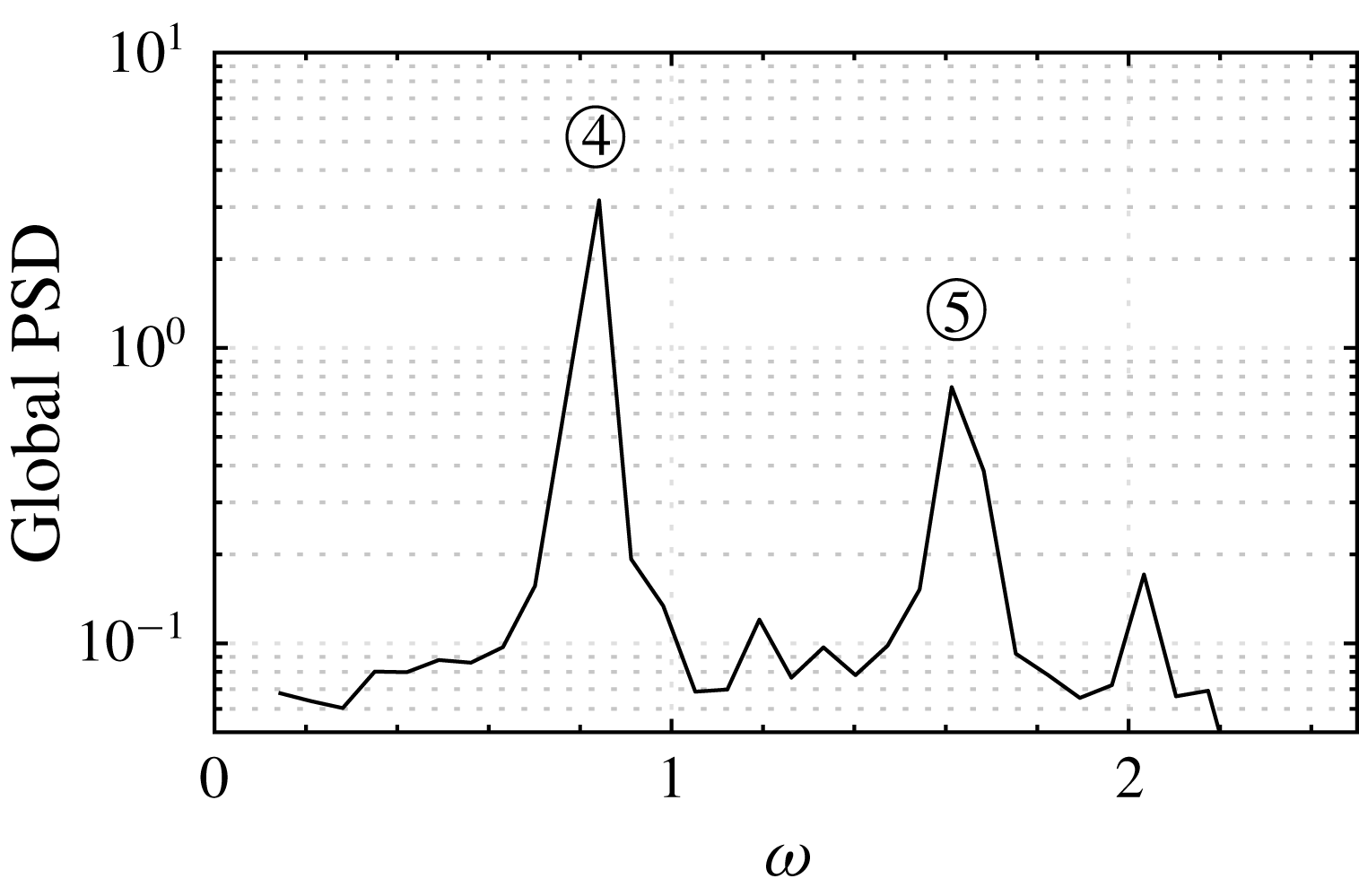
to focus on the synchronization in the supercritical region. Figure 12 shows the frequency spectrum for this configuration. Again, there are two dominant peaks, here at
 $\unicode[STIX]{x1D714}=0.84$
and
 $\unicode[STIX]{x1D714}=1.61$
. The respective Fourier modes are presented in figure 13. The mode
 $\unicode[STIX]{x1D714}=0.84$
in figure 13(a) indicates a sinuous oscillation very similar to the observation in figure 11(b). Likewise, the second mode,
 $\unicode[STIX]{x1D714}=1.61$
shows a varicose oscillation in figure 13(b). Apparently, the existence of both sinuous and varicose modes can be confirmed in this second experiment. Again, the varicose mode fluctuates at the first harmonic frequency of the sinuous mode.
In the last experiment, the ability of sinuous and varicose eigenmodes to deviate from their natural frequency is investigated by forcing the flow with controlled harmonic waves. For this investigation, the configuration
 $(\unicode[STIX]{x1D702},x_{k})=(1,57.1)$
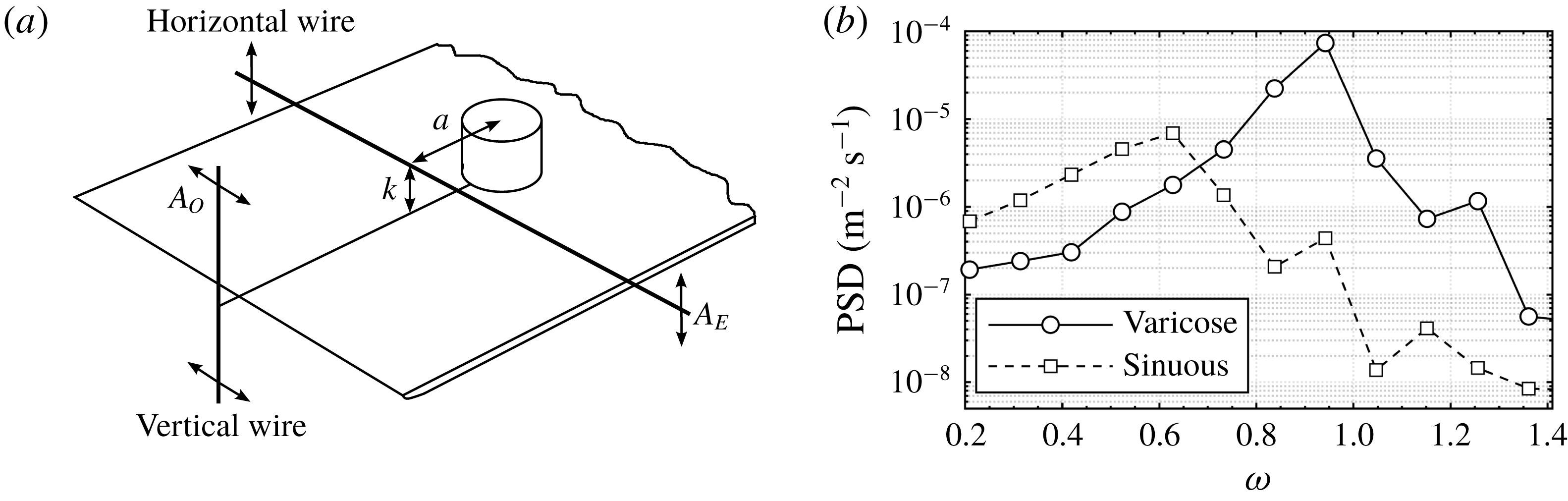
is extended with two mechanical disturbance sources to force the flow at various frequencies. The first disturbance source is a horizontal vibrating wire for symmetric forcing and the other one is a vertical vibrating wire for antisymmetric forcing. Figure 14(a) illustrates a sketch of the modified set-up with both disturbance sources. The horizontal wire is made of stainless steel with a diameter of 0.1 mm and is spanned across the spanwise direction at
 $(x,y)=(-10,1)$
. The streamwise position is also indicated by
 $a$
in figure 14(a). Two stepper motors oscillate the wire harmonically with an amplitude of
 $A_{E}=\pm 0.25~\text{mm}$
. The vertical wire has a diameter of 1 mm and is placed upstream of the leading edge. Its oscillation amplitude is as large as
 $A_{O}=\pm 10~\text{mm}$
, but shear sheltering prevents the majority of this disturbance from entering the boundary layer. A detailed introduction, testing and application of the disturbance sources is provided in Puckert (Reference Puckert2019). The Reynolds number in this investigation is in the subcritical regime at
 $Re_{k}=620$
and the probe is placed at
 $(x,y,z)=(10,1,0)$
.
Global power spectrum density from Fourier decomposition for
 $(\unicode[STIX]{x1D702},x_{k})=(1,166.4)$
at
 $Re_{k}=1230$
.
Fourier mode of
 $\pm 0.1$
of maximum streamwise perturbation at (a)
 $\unicode[STIX]{x1D714}=0.84$
and (b)
 $\unicode[STIX]{x1D714}=1.61$
at
 $Re_{k}=1230$
. For spectrum see figure 12 numbers
 $\unicode[STIX]{x2463}$
and
 $\unicode[STIX]{x2464}$
, respectively.

In this experiment, 12 equally spaced forcing frequencies between
 $0.2<\unicode[STIX]{x1D714}<1.4$
are applied with separate horizontal and vertical disturbance input, respectively. The PSD at the forcing frequency is obtained from discrete Fourier transforms. The combined result of these experiments is shown in figure 14(b). It illustrates the response of the system to harmonic forcing and is thus a measure for the sensitivity of the flow. The figure reveals interesting features by looking at the peaks of the respective curves and their widths. As expected, the flow is sensitive to symmetric disturbances in the vicinity of
 $\unicode[STIX]{x1D714}=1$
, close to the predicted varicose mode. Similarly, the antisymmetric forcing experiences largest amplification close to the predicted sinuous mode. The width of the sensitive regions in figure 14(b) demonstrates that both modes can deviate relatively far from their theoretically predicted eigenfrequency in the presence of controlled forcing input. This result supports the explanation that the varicose mode and the sinuous mode can lock together at supercritical Reynolds numbers through the exchange of energy. This process tends to be in favour of the sinuous mode at supercritical Reynolds numbers due to its self-sustaining nature.
Harmonic forcing: (a) revised set-up with two disturbance wires and (b) response at different frequencies at
 $Re_{k}=620$
.
4.1 Discussion
The PIV results in this section confirm that both sinuous and varicose modes adjust themselves to each other. Since ‘synchronization’ is a term often used in the literature, some remarks on the terminology are given. From a theoretical point of view, synchronization requires all participating modes to be self-oscillators (Pikovsky et al. Reference Pikovsky, Rosenblum, Kurths and Kurths2003). In the present study, both varicose and sinuous modes are solutions to the eigenvalue problem of this system. When physical flows are considered, there is a small remaining level of turbulence intensity which suffices to trigger the highly sensitive varicose mode. When regarding the slightly disturbed system, the varicose mode quasi-resonates and thus qualifies for the term ‘synchronization’ with the sinuous mode. This is similar to the oscillation of a circular cylinder in the von Kármán vortex street, where the mechanical system can lock to the intrinsic vortex shedding of the self-induced wake. Although the mechanical part of this system is linearly stable and forced by the vortex street, most authors agree on the term synchronization to describe the high oscillation amplitudes of vortex-induced vibrations in a certain frequency range (Griffin & Ramberg Reference Griffin and Ramberg1974; Govardhan & Williamson Reference Govardhan and Williamson2000; Gabbai & Benaroya Reference Gabbai and Benaroya2005; Meliga & Chomaz Reference Meliga and Chomaz2011).
Since synchronization requires an exchange of energy between the respective modes, it may be hypothesized that the energy of the sinuous mode suffices to trigger the varicose mode. In a disturbance-free environment, such a scenario is plausible, because the wavemaker region of the sinuous mode in the recirculation zone is very close to the high wall-normal shear that is responsible for the varicose mode (Loiseau et al. Reference Loiseau, Cherubini, Robinet and Leriche2014; Citro et al. Reference Citro, Giannetti, Luchini and Auteri2015). This question might be answered with low-order physical models. For the case of vortex-induced vibrations, for instance, Facchinetti, De Langre & Biolley (Reference Facchinetti, De Langre and Biolley2004) used the van der Pol equation to describe the vortex shedding and introduced coupling terms between the mechanical system and the flow. Similarly, Meliga & Chomaz (Reference Meliga and Chomaz2011) applied an asymptotic expansion approach to successfully predict the synchronization effect in vortex-induced oscillations. The later approach seems promising for the theoretical prediction of the fluid–fluid interaction observed in the present experiment. The present work thus provides space for future investigations on this fascinating topic.
5 Conclusions
Hot-film anemometry and particle image velocimetry have been performed in a laminar water channel to investigate the flow downstream of a cylindrical roughness element in a laminar boundary layer. Three different roughness elements are considered with aspect ratios
 $\unicode[STIX]{x1D702}=1$
and
 $\unicode[STIX]{x1D702}=3$
. The experiments demonstrate that for
 $\unicode[STIX]{x1D702}=1$
, two modes of different symmetry adjust their frequency with each other and oscillate synchronously. Due to the self-sustained nature of the oscillation and weak coupling of the two modes, this mechanism may be referred to as synchronization. To the knowledge of the authors, no observation of this important mechanism has been reported in boundary layers before.
In the subcritical regime of the case
 $\unicode[STIX]{x1D702}=1$
, only a convective varicose mode is observed. As the Reynolds number is increased beyond the critical Reynolds number, the system becomes globally unstable due to a sinuous mode at a different frequency than the original convective mode. This is confirmed by 3-D global linear stability theory. In our physical experiment, the frequency of the convective mode is locked to the frequency of the first harmonic of the sinuous mode at supercritical Reynolds numbers due to nonlinear interaction (weak coupling). As a result, the flow consists of a sinuous fundamental oscillation with a varicose higher harmonic. This unexpected observation is confirmed by another experiment at a different roughness position in the laminar boundary layer and further substantiated by artificial forcing of the flow. The observations in the present work substantiate the idea of synchronization of boundary-layer modes. The configuration
 $\unicode[STIX]{x1D702}=3$
was introduced as a case of large aspect ratio where the varicose mode dominates both convective and global instabilities. If only one dominant mode is present, synchronization is not necessary and therefore not observed in the experiment.
Acknowledgements
We thank J.-Ch. Robinet, S. Cherubini and M. A. Bucci for discussions on global instability.


 Open access

