NOMENCLATURE
- A
-
cross-sectional area
- AR
-
wing aspect-ratio
- b
-
wing span
- B
-
linear strain-displacement matrix
- BNL
-
non-linear strain-displacement matrix
- c
-
chord
- croot
-
wing-root chord
- ctip
-
wing-tip chord
- Cf
-
friction drag coefficient
- CD
-
drag coefficient
- C Df
-
correction factor for the friction drag coefficient
- CL
-
lift coefficient
- C L α
-
lift coefficient slope
- CM
-
pitch moment coefficient
- C p, 0
-
incompressible pressure coefficient
- CP
-
pressure coefficient
- d
-
nodal displacement vector
-
 $\dot{d}$
-
nodal velocity vector
-
$\ddot{d}$
-
nodal acceleration vector
- D
-
elasticity matrix
- E
-
Young’s modulus
- EI
-
bending stiffness
- EIyy
-
bending stiffness in y axis (flap bending stiffness)
- EIzz
-
bending stiffness in z axis (chord bending stiffness)
- F
-
total load vector
- Fg
-
gravity load vector
- FF
-
form factor
- g
-
gravity acceleration
- G
-
shear modulus
- GJ
-
torsional stiffness
- I 2/I 1
-
inertia ratio
- K
-
stiffness matrix
- M
-
mass matrix
- M ∞
-
free-stream Mach number
- n
-
normal vector to the surface
- N
-
shape function matrix
- NN
-
number of structural nodes
- p
-
pressure
- p ∞
-
free-stream reference pressure
- r
-
distance between a point and the source or doublet location
- R
-
vector of restoring forces
- S
-
wing area
- Sref
-
wing reference area
- Swet
-
wing wetted area
- SB
-
surface boundary
- t
-
time
- T
-
kinetic energy
- u
-
displacement vector
- ux
-
displacement in chord direction
- uz
-
displacement in out-of-wing-plane direction
- uz /(b/2)
-
dimensionless vertical tip displacement
- U
-
potential energy
- vrel
-
additional relative motion
- V
-
velocity
- V ∞
-
free-stream velocity
- α
-
angle-of-attack
- δ
-
source strength
- ε
-
strain vector
- θ y
-
angle of twist
- λ
-
wing taper-ratio
- μ
-
doublet strength
- μ l
-
doublet strength at the lower surface of the trailing edge
- μ u
-
doublet strength at the upper surface of the trailing edge
- ρ
-
air density
- σ
-
stress vector
- Φ
-
potential
- Φ∞
-
free-stream potential
- ω
-
natural frequency
- Ω
-
rate of rotation


Greek Symbol
1.0 INTRODUCTION
Currently, the aeronautical industry is striving to improve aircraft performance while reducing environmental impact. These goals are contradictory. There is, however, a commonly used metric associated with both objectives: fuel consumption. In general, aircraft designs with lower fuel consumptions are more efficient and present a lower environmental signature. Several aircraft concepts claim to substantially enhance flight efficiency(Reference Abbas, de Vicente and Valero1,Reference Barbarino, Bilgen, Ajaj, Friswell and Inman6,Reference Liebeck31,Reference Stanewsky53,Reference Wolkovitch62) . Among the parameters changed by aircraft designers to achieve flight efficiency is the increase in wing aspect-ratio. This specially applies to original equipment manufacturers, which are under pressure for reducing the environmental impact of their products and at the same time provide with competitive operational cost.
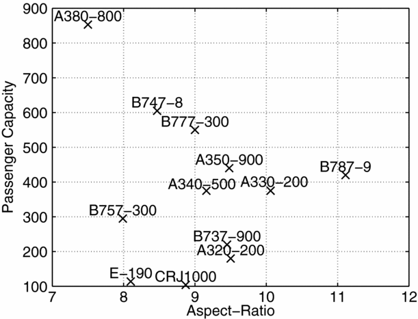
Aircraft with high aspect-ratios provide a higher lift-to-drag ratio and longer range, thus enhancing aircraft performance(Reference Abbott and Von Doenhoff2). Despite the knowledge of such improvement in flight efficiency, commercial jets commonly have relatively low aspect-ratios (no higher than 12, see Fig. 1). This is partially explained by the large deformations that are characteristic of flexible wings under normal operating conditions, which lead to geometrical non-linear behaviour and possibly to aeroelastic problems(Reference Cooper and Harmin18): large wing deformations may alter the natural frequencies and mode shapes and, consequently, the aeroelastic behaviour of the wing(Reference Patil, Hodges and Cesnik42). Hence, it is of prime importance to study the influence of such non-linearities on the aeroelastic behaviour, namely on the occurrence of aeroelastic instabilities such as divergence or flutter. The structural flexibility increase does not only change the aeroelastic behaviour of the wing, but also may lead to instabilities in flight dynamics such as higher sensibility to disturbances (e.g. gusts) and coupling between rigid-body modes and structural dynamic modes (aeroservoelasticity)(Reference Livne and Weisshaar32).
Main aircraft wing aspect-ratios. Data collected from the airliners’ manufacture websites.

The non-linear aeroelastic analysis of a very flexible wing may be done in either the frequency or the time domain. Several numerical works have been published over the past few decades using low-/medium-fidelity models for the non-linear aeroelastic analyses of high-aspect-ratio wings and highly flexible aircraft at low subsonic conditions. The structural models used consist in general of analytic(Reference Arena, Lacarbonara and Marzocca4,Reference Dowell and Tang19,Reference M J Patil and Cesnik33,Reference Patil and Hodges40) or finite element beam models(Reference Kampchen, Dafnis, Reimerdes, Britten and Ballmann28) with constant geometry and material properties. The aerodynamic models employed in these studies use doublet-lattice method (DLM)(Reference Patil and Hodges40) and 2D unsteady aerodynamics models(Reference M J Patil and Cesnik33) with flow separation prediction(Reference Arena, Lacarbonara and Marzocca4,Reference Dowell and Tang19,Reference Dunn and Dugundji21) .
In order to study the non-linear aeroelastic behaviour coupled with flight dynamics in highly flexible aircraft, a time-marching computational model that couples non-linear aeroelasticity with flight dynamics and considers the complete aircraft is required. The ASWING(Reference Drela20), NATASHA(Reference Chang, Hodges and Patil16,Reference Patil39,Reference Patil and Hodges41,Reference Sotoudeh and Hodges51) , UM/NAST(Reference Cesnik and Brown13,Reference Cesnik and Brown14,Reference Shearer and Cesnik48,Reference Su and Cesnik54,Reference Su and Cesnik56) , NANSI(Reference Wang, Chen, Liu and Mook61) and SHARP(Reference Hesse and Palacios24,Reference Murua, Palacios and Graham36,Reference Simpson, Palacios and Murua49) frameworks were specially developed to analyse very flexible aircraft, particularly High-Altitude Long Endurance (HALE) aircraft. These frameworks and others have been applied to study non-linear flight dynamics in terms of dynamic response(Reference Shearer and Cesnik48,Reference Su and Cesnik55,Reference Su and Cesnik56) , stability analysis(Reference Patil and Hodges41,Reference Raghavan and Patil44,Reference Su and Cesnik55,Reference Su and Cesnik56) , flutter boundary(Reference Su and Cesnik55) and gust response(Reference Cook, Palacios and Goulart17,Reference Patil39,Reference Su and Cesnik55,Reference Su and Cesnik56) of highly flexible aircraft. Palacios et al(Reference Palacios, Murua and Cook38) compared the available aerodynamic and structural models used for analysing very flexible low-speed aircraft.
Despite the large number of numerical studies, just a few experimental analyses related to non-linear aeroelasticity of high-aspect-ratio wings are available in the literature. All known experimental data found is based on simple planar straight wings at low subsonic speeds, with highly flexible structures designed to: deform significantly(Reference Dunn and Dugundji21,Reference Kampchen, Dafnis, Reimerdes, Britten and Ballmann28) ; exhibit flutter and limit cycle oscillation (LCO) under aerodynamic loading at speeds within the range of the wind tunnel where they are going to be tested(Reference Tang and Dowell57,Reference Tang and Dowell59) ; study gust response(Reference Tang and Dowell58,Reference Tang, Grasch and Dowell60) . Some of these studies include the effect of slender bodies at the wing tip or at different span-wise positions, which in general causes reduction of the frequency of the first torsional mode of vibration. Cesnik et al(Reference Cesnik, Senatore, Su, Atkins and Shearer15) develop an 8 m wingspan HALE aircraft model, named X-HALE, aiming to provide experimental data for code validation with coupled non-linear aeroelasticity and flight dynamic modes, although no experimental data was yet published.
Since the available experimental data is scarce, many model validations are performed with the same experimental data obtained from literature, namely the data published by Tang and Dowell(Reference Tang and Dowell57) for a wing with an aspect-ratio of approximately 18, or analytic and experimental data from studies conducted during the last half-century on wings with much lower aspect-ratios(Reference Goland and Buffalo22,Reference Yates64) .
For this work, a non-linear aeroelastic framework capable of analysing the aeroelastic behaviour of high-aspect-ratio wings, taking into account geometric non-linearities, was developed and benchmarked. In order to benchmark the static non-linear solver developed for this study, experimental data reported by Tang and Dowell(Reference Tang and Dowell57) was used.
The main objective of this paper is to evaluate the aeroelastic benefits of increasing wing aspect-ratio by means of reducing wing chord or, alternatively, decreasing taper ratio. With this in mind, a rectangular wing with a span of 20 m and a chord of 1 m was used as baseline model for this work. To increase wing aspect-ratio, these two approaches were compared in terms of aerodynamic induced drag, root bending moment and flutter boundary.
2.0 DEVELOPED FRAMEWORK/METHODOLOGY
A computational framework was developed, in the scope of EU FP7 NOVEMOR project, aiming at incorporating in a multidisciplinary design optimisation (MDO) environment with the capabilities of analysing the two objectives of the project: morphing solutions and novel configurations. To expand the applications of this tool in preliminary aircraft design, an aeroelastic module was developed with the capability of modelling linear and non-linear, steady and unsteady (time domain) aeroelastic analyses.
The models included in aeroelastic module are of low/medium fidelity: (1) the aerodynamic model is based on a 3D panel method code that takes into account a compressibility correction and estimates the viscous drag in the model; (2) the structural model consists of a 3D condensed beam model, which represents the structural stiffness and mass distributions along the wing span by calculating the properties EIyy and EIzz of the span-wise wing cross-section. The non-linear structural features are restricted to geometric and stress-stiffening non-linearities, while the aerodynamic non-linearities are purely geometrical, in the sense that they are caused not by viscous effects or shocks but purely by the structural displacement. A brief description of these models is presented next.
2.1 Aerodynamic model
Since the developed framework’s main aim is preliminary aircraft design, a fast estimation of aerodynamic loads that adequately accounts for the fluid behaviour in aeroelastic computations is desired. For this reason, a potential flow model was used, which provides accurately the lift loading and allows computing critical aeroelastic instabilities such as flutter or divergence speeds in incompressible and low compressibility regimes (up to Mach 0.65, if a suitable correction is employed, e.g. Prandtl-Glauert) and when viscous effects are minimal (i.e. no boundary-layer separation occurs).
2.1.1 Problem formulation
The implemented potential flow model consists of a three dimensional panel code based on the formulation described in Katz and Plotkin(Reference Katz and Plotkin29). In the panel method formulation, the flow is assumed to be incompressible, inviscid and irrotational. Considering these assumptions, the governing equation can be written in terms of velocity potential, Φ(x, y, z), by the Laplace’s equation:
 $$\begin{equation}
\nabla ^2\Phi = 0.
\end{equation}$$
2.1.2 Steady formulation
To solve the Laplace’s equation, two boundary conditions are prescribed:
-
• impermeability condition (zero normal velocity on a body),
-
• far field condition (the motion should disappear far from the body).
The Laplace’s equation (Equation (1)) is linear differential and, thus, it has several possible analytical solutions. One of them consists in applying Green’s Theorem to build a solution based on the distribution of sources and doublets on the problem boundaries (body and wake) yielding the following solution(Reference Katz and Plotkin29):
 $$\begin{equation}
\Phi \left(x,y,z\right)=\frac{-1}{4\pi }\int _{S_B}\left[\delta \left(\frac{1}{r}\right)-\mu \; \textrm {n}\cdot \nabla \left(\frac{1}{r}\right)\right]dS + \Phi _{\infty },
\end{equation}$$
where δ and μ are, respectively, the source and doublet strength, r is the distance between the point (x, y, z) and the source/doublet location,
 $\textrm {n}$
is the normal vector to the surface, SB
the surface boundary and Φ∞ the free-stream potential.
The numerical panel method based on the formulation described in Katz and Plotkin(Reference Katz and Plotkin29) uses elements with constant intensity sources and doublets distributions. The application of these elements fulfills the far field boundary condition. However, to satisfy the impermeability condition, one has to impose one of three boundary conditions: (1) Neumann boundary condition; (2) Dirichlet boundary condition; or (3) mixed boundary condition. For the developed panel code, the Dirichlet boundary condition was used, which prescribes the total potential inside the surface as Φ = Φ∞ and is the equivalent to state that the inner perturbation potential is zero. Equation (2) can then be expressed in the form:
 $$\begin{equation}
\frac{1}{4\pi }\int _{body+wake}\mu \frac{\partial }{\partial \textrm {n}}\left(\frac{1}{r}\right)dS -\frac{1}{4\pi }\int _{body}\delta \left(\frac{1}{r}\right)dS = 0.
\end{equation}$$
For this equation (Equation (3)) to have one particular solution, the source strength for solid bodies boundaries is prescribed to be:
 $$\begin{equation}
\delta =-{\rm n}\cdot \nabla \Phi _{\infty }.
\end{equation}$$
The wake is modelled as a constant doublet distribution, which strength is obtained by applying the Kutta condition:
 $$\begin{equation}
\mu =\mu _u-\mu _l,
\end{equation}$$
where μ u and μ l are, respectively, the doublet strengths at the upper and lower surfaces of trailing edge from which the wake element is shedding.
To solve this problem, one has to discretise the body surface and wake into several panels. The so-called aerodynamic influence coefficients were evaluated by computing the surface integrals in Equation (3) for each collocation point (placed at the centre of each panel). Since the source’s and doublets’ strengths are considered constant for each panel, the integrals depend only on the geometry. The doublet distribution (μ k ) is differentiated using a second order central differentiation scheme to compute the tangential velocity (V) at the collocation points. The pressure (p) on each panel can be computed from Bernoulli’s equation for potential flow, assuming, as reference, the free-stream velocity (V ∞):
 $$\begin{equation}
\frac{p_{\infty }-p}{\rho }=\frac{V^2}{2}-\frac{V_{\infty }^2}{2}+\frac{\partial \Phi }{\partial t},
\end{equation}$$
where p ∞ and ρ denote free-stream reference pressure and air density, respectively. The incompressible pressure coefficient (C p, 0) can then be calculated for the steady case (∂Φ/∂t = 0) by,
 $$\begin{equation}
C_{p,0} = \frac{p-p_{\infty }}{\frac{1}{2}\rho V_{\infty }^2} = 1 - \frac{V^2}{V_{\infty }^2}.
\end{equation}$$
The pressure values for each panel are integrated over the surface to compute the total body pressure forces. Aiming at improving the accuracy of pressure estimation for higher subsonic flows, the Prandtl-Glauert rule(Reference Bertin11) is applied, resulting in a corrected pressure coefficient,
 $$\begin{equation}
C_{p} = \frac{C_{p,0}}{\sqrt{1-M_{\infty }^2}},
\end{equation}$$
where M ∞ denotes the free-stream Mach number. A friction coefficient (Cf ) and form factor (FF) for drag correction (C Df ), considering the wing wetted and reference areas (Swet and Sref , respectively), was also implemented to account for viscous effects,
 $$\begin{equation}
C_{D_f} = C_fFF\frac{S_{wet}}{S_{ref}}.
\end{equation}$$
A detailed description of this correction (flat plate zero pressure gradient friction drag-based calculation) can be found in the literature(Reference Mason34).
2.1.3 Unsteady formulation
Despite the previous described methodology not accounting for time dependent terms, it is possible to perform small modifications to include them(Reference Katz and Plotkin29). Laplace’s equation (Equation (1)) is still valid for the unsteady case(Reference Katz and Plotkin29), although slight alterations are performed to its boundary conditions:
-
• the impermeability condition is now called “zero normal flow on a solid surface” boundary condition and it depends on the local surface velocity;
-
• the far field condition is maintained;
-
• and, a new condition, known as Kelvin condition, depending on vortex strength, (which can be related to doublet strength) is required to determine the stream-wise variation with time of the strength of the vorticity shed into the wake.
For convenience, the unsteady motion is described in a body-fixed coordinate system on which “zero normal flow on a solid surface” boundary condition is applied. The body-fixed coordinate system is assumed to be known and is written in reference to the inertial frame. At t = 0, both coordinate systems coincide; while for t > 0, the relative motion of the body-fixed coordinate system origin is described by its location and orientation. The “zero normal flow on a solid surface” boundary condition can be rewritten in terms of the velocity (V 0) and rate of rotation (Ω) of the body-fixed coordinate system:
 $$\begin{equation}
\left(\nabla \Phi -V_0-v_{rel}-\Omega \times r\right)\cdot \textrm {n}=0,
\end{equation}$$
with vrel representing additional relative motion (e.g. in case of small oscillations or deformation speeds).
As for the steady case, the numerical panel methods use elements with constant intensity sources and doublets distributions, which fulfills the far field boundary condition. However, to fulfill the “zero normal flow on a solid surface,” the Dirichlet boundary condition can be applied as in the steady case. One can also rewrite the solution of Laplace’s equation similarly to Equation (3), but now the source strength for solid bodies becomes:
 $$\begin{equation}
\delta =-{\rm n}\cdot \left(V_0+v_{rel}+\Omega \times r\right).
\end{equation}$$
The wake model is not fixed as in the steady case; in fact, it increases in length (number of wake panels) with time and respects the following conditions:
-
• no vorticity is added in the wake, Kelvin condition;
-
• at each time step, the doublet strength is computed by applying Kutta condition (Equation (5)) at aerofoil trailing edges;
-
• each wake panel length is computed by multiplying the time step (Δt) by the free-stream velocity (V ∞).
Considering now the time derivative in the Bernoulli’s equation (Equation (6)), one can calculate the incompressible pressure coefficient for the unsteady case,
 $$\begin{equation}
C_{p,0} = 1 - \frac{V^2}{V_{\infty }^2}-\frac{2}{V_{\infty }^2}\frac{\partial \Phi }{\partial t}.
\end{equation}$$
To solve this equation, a time discretisation method is required and since the objective is to compute the pressure coefficient at the time instance t + Δt, this method has to be implicit. One of the most commonly used, and the one implemented, is the Backward Euler Method(Reference Hirsch25), which is first order accurate and when applied to Equation (12) yields,
 $$\begin{equation}
C_{p,0}^{t+\Delta t} = 1 - \frac{\left(V^{t+\Delta t}\right)^2}{V_{\infty }^2} - \frac{2}{V_{\infty }^2}\left(\frac{\Phi ^{t+\Delta t}-\Phi ^t}{\Delta t}\right).
\end{equation}$$
The pressure values for each panel are integrated over the surface to compute the total body pressure forces. The compressibility and viscous drag corrections (Equation (8) and Equation (9), respectively) are also used in the unsteady formulation in order to improve the pressure and drag estimation accuracy.
2.1.4 Benchmarking
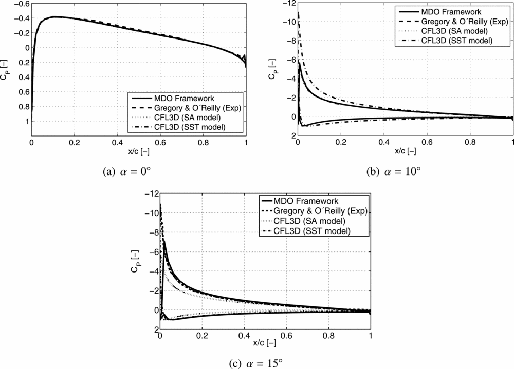
The implemented aerodynamic model (steady formulation) was compared in terms of chord-wise pressure coefficient, Cp , not only with experimental data(Reference Gregory and O’Reilly23), but also with numerical results, for a NACA 0012 aerofoil(37). Two turbulence models were used for this comparison: Spalart-Allmaras (SA)(Reference Spalart and Allmaras52); and standard Menter shear stress transport (SST)(Reference Menter35). For extracting the data in the developed framework, a wing with a high aspect-ratio (20 m of span and a chord of 1 m) was defined and the chord-wise CP distribution was computed near the wing root for three different angles-of-attack: 0°, 10° and 15°. A Mach number of 0.2 (incompressible flow) and sea level altitude conditions were considered.
One can observe from Fig. 2 that the results obtained with the developed aerodynamic model are in good agreement with the experimental and numerical results for the chord-wise pressure coefficient distribution. A note should be made regarding the drag coefficient. As mentioned earlier, the Panel Method is inviscid, which leads to a lower drag coefficient prediction. It can be seen that for higher angles of attack (Fig. 2(c)) there is a slight deviation from the obtained chord-wise CP distribution and the experimental values. This difference is expected to be more evident if CD was plotted instead of CP since the panel code does not properly take into account viscous effects, and at this angle-of-attack, there is flow separation.
Comparison of the chord-wise pressure coefficient distribution with experimental(Reference Gregory and O’Reilly23) and numerical results(37).

2.2 Structural model
The structural model is a condensed 3D beam model, also known as “beam-like” model. This model is widely applied for preliminary aircraft design since it allows capturing some of the most important structural responses at a low complexity and computational cost. However, the direct application of beam elements to represent the wing can lead to some inaccuracies (namely, the poor representation of stiffness and moments of inertia), which are not acceptable for higher-fidelity levels. With this in mind, a more accurate model that accounts for structural stiffness and mass characteristics of “box-like” components (e.g. wing-box)(Reference Wright and Cooper63) was implemented and condensed in a “beam-like” model. Furthermore, for the study of high-aspect-ratio wings, the wing structure behaviour is similar to a “beam-like” structure. A wing-box is defined for each aerofoil section in terms of its chord-wise initial and final position, besides web and cap thicknesses. Using thin-wall theory and the parameterised wing-box data, the inertial properties (area and moments of inertia) and centroid are computed. The condensed beam model is then set to pass through the centroids of each aerofoil section.
2.2.1 Problem formulation
The structural model is based on the finite element method (FEM) to describe the condensed 3D beam model. The implemented finite element is a 3D thin/slender beam element(Reference Soares50) based on the Euler-Bernoulli beam theory(Reference Reddy45) and composed of two nodes with six degrees-of-freedom (DOFs) each. This model consists of assembling four decoupled elements: one bar; two beams (one for each bending plane); and one torsion. The displacement field, {u}, which includes both displacements and rotations, can be defined for the assembled 3D beam element as a function of the shape function matrix, [N], and the nodal displacements, {d}, by the following expression:
 $$\begin{equation}
\lbrace u\rbrace = [N] \lbrace d\rbrace .
\end{equation}$$
The strain field, for this element, is composed of the axial strain, two bending curvatures (planes xy and xz) and twist angle; and can be defined in terms of strain-displacement matrix, [B], and nodal displacements as follows:
 $$\begin{equation}
\lbrace \epsilon \rbrace = [B] \lbrace d\rbrace .
\end{equation}$$
For this element, the stress field is also modified. It includes axial force and bending moments in the three planes. Furthermore, the material is assumed to be isotropic and elastic, which results in the following stress field:
 $$\begin{equation}
\lbrace \sigma \rbrace = [D] \lbrace \epsilon \rbrace ,
\end{equation}$$
where [D] is the elasticity matrix. A brief description of the finite element method implemented in the structural model, whose formulation is based on the variational method, is presented next.
2.2.2 Static analysis
The potential energy, U, of the beam finite element is given by,
 $$\begin{equation}
U = \frac{1}{2}\lbrace d\rbrace ^T[K]\lbrace d\rbrace - \lbrace d\rbrace ^T\lbrace F\rbrace ,
\end{equation}$$
where [K] and {F} are the stiffness matrix and total load vector of the element, respectively. The stiffness matrix and load vector are written in the element coordinate system. A transformation matrix is required to compute both this matrix and vector in the global coordinate system and allow assembling all the finite elements.
The static equilibrium is obtained by applying the principle of virtual work, yielding that the potential energy is stationary, with respect to the nodal displacements:
 $$\begin{equation}
\frac{\partial U}{\partial \lbrace d\rbrace } = 0 \Rightarrow [K]\lbrace d\rbrace =\lbrace F\rbrace .
\end{equation}$$
To solve this system of equations, an in-house linear solver that automatically selects the most suitable decomposition (LU, QR and Cholesky are possible) to invert the stiffness matrix is used.
2.2.3 Dynamic analysis
In a dynamic analysis, not only the elastic deformation is accounted for, but also the inertial properties are considered (the beam element model does not take into account damping). Therefore, it is necessary to compute the kinetic energy, T:
 $$\begin{equation}
T = \frac{1}{2}{\lbrace \dot{d}\rbrace }^T[M]{\lbrace \dot{d}\rbrace },
\end{equation}$$
where [M] is the mass matrix of the element. The nodal velocity vector,
 ${\lbrace \dot{d}\rbrace }$
, is the time derivative of nodal displacement vector.
The potential energy is represented analogously to the one presented in the static analysis, although now the displacements and forces are in function of both time and space. For the dynamic equilibrium of the element in Lagrangian formulation, the equation is
 $$\begin{equation}
\frac{d}{dt}\left(\frac{\partial T}{\partial {\lbrace \dot{d}\rbrace }}\right) + \frac{\partial U}{\partial \lbrace d\rbrace } = \left\lbrace 0\right\rbrace \Rightarrow [M]{\lbrace \ddot{d}\rbrace } + [K]\lbrace d\rbrace = \lbrace F\rbrace ,
\end{equation}$$
where the vector of accelerations,
 ${\lbrace \ddot{d}\rbrace }$
, is given by second order time derivative of the displacement vector. To solve this system, a time integration scheme is required and for the developed framework, both Newmark(Reference Bathe7) and Bathe(Reference Bathe and Noh8) methods were implemented. For the case of modal free-vibration analysis, there is no force applied; therefore, the equation of dynamic equilibrium is now an eigenvalue and eigenvector problem:
 $$\begin{equation}
[K]\lbrace d\rbrace =\omega ^2[M]\lbrace d\rbrace .
\end{equation}$$
An in-house eigensystem solver is used to compute the eigenvalues and eigenvectors of this problem.
2.2.4 Non-linear analyses
Aiming at enabling the model with the capability of incorporating geometric non-linearities, a few changes to both static and dynamic analyses were performed.
The stiffness matrix is now dependent of the deformed state; thus, in order to reach the non-linear static equilibrium at a given time step, t + Δt, an iterative method is required. The one implemented is the full Newton-Raphson method(Reference Bathe7), which aims at reaching the following equilibrium:
 $$\begin{equation}
^{t+\Delta t}\lbrace F\rbrace -^{t+\Delta t}\lbrace R\rbrace ^i=\lbrace 0\rbrace ,
\end{equation}$$
where the applied load, {F}, does not depend on the deformation, but the restoring force {R} does, with i being the current iteration. These restoring forces are the internal structural nodal forces, which are computed from the previous iteration stiffness matrix as follows:
 $$\begin{equation}
^{t+\Delta t}\lbrace R\rbrace ^i=^{t+\Delta t}[K]^{\left(i-1\right)}\lbrace d\rbrace ^i.
\end{equation}$$
There are different approaches to treat large displacements and large rotations, although for the developed framework, NASTRAN™ methodology(Reference Lee30) was followed. It consists in computing the net displacements and using the gimbal angle approach to treat, respectively, large displacements and large rotations. The implemented non-linear model does not account for large strains.
Since the main objective of this aeroelastic framework is to study high-aspect-ratio wings, where flexibility effects are of high importance, the element weight is also considered in the model. To do so, the gravity load, {Fg }, is computed by multiplying the mass matrix by the gravity acceleration vector, {g}:
 $$\begin{equation}
\lbrace F_g\rbrace =[M]\lbrace g\rbrace .
\end{equation}$$
Stress stiffening effects can also be modelled, if one considers a non-linear component on the strain-displacement matrix:
 $$\begin{equation}
\lbrace \epsilon \rbrace = \left([B] + [B_{NL}]\right) \lbrace d\rbrace ,
\end{equation}$$
where the strain-displacement matrix has now a non-linear component, [BNL ]. Besides the linear stiffness matrix, two more matrices can be computed: the large displacement stiffness matrix and the geometric stiffness matrix. The former is usually neglected(Reference Soares50), while the latter can be conveniently transformed as a function of stress state(Reference Zienkiewicz65).
2.2.5 Benchmarking
The structural model is a low-/medium-fidelity model consisting of an equivalent beam model, as already mentioned. For the purpose of validation, NASTRAN™ software was used. The problem devised for the benchmarking consists in a
 $10\,\text{m}$
aluminum (with a Young modulus of
 $70\,\text{GPa}$
, a density of
 $2,700\,\text{kg/m}^3$
and a shear modulus of
 $27\,\text{GPa}$
) cantilever beam with a width and a height of
 $0.2\,\text{m}$
and
 $0.1\,\text{m}$
, respectively.
Different magnitudes of vertical loads were applied on the beam tip to evaluate the performance of the developed tool. The beam’s self-weight was accounted for in the calculations. Only constant forces were applied in the non-linear study. A uniform mesh of 500 co-linear CBEAM elements representing the cross-section was used for NASTRAN™ computations.
Both linear and non-linear static analyses presented very good agreement between the results from the MDO framework and NASTRAN™: a maximum error of 0.03% for the displacements and 0.26% for the maximum stress (for the load value) were reached for the non-linear solution. The main difference between NASTRAN™ and the implemented framework is in terms of non-linear solution convergence. While the developed tool updates the stiffness matrix in each iteration, using a full Newton-Raphson method(Reference Bathe7), NASTRAN™ does not perform a stiffness matrix update in every iteration, but employs a modified Newton-Raphson method instead. For this specific case, only one load step was required for both codes and both equilibrium and convergence were reached.
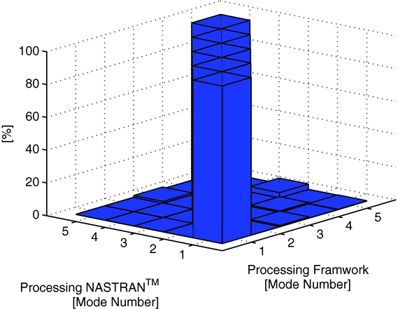
The same cantilever beam was also used in verifying the quality of the free-vibration analysis of the framework relative to the NASTRAN™ solution. Twelve mode shapes and the corresponding frequencies were extracted and compared: the relative errors for natural frequencies are very low (below 0.01%); and the mode shapes also exhibit very good agreement when one computes the coordinate modal assurance criterion (COMAC)(Reference Allemang3) to compare both solutions (see Fig. 3).
Comparison of the first five mode shapes using COMAC.

A structural dynamic test case was also devised to compare the performance of linear and non-linear dynamic solvers. This test case consists of a cantilever beam (with a length of 0.2540 m and a square cross-section with
 $0.0254\,\text{m}$
sides) with a uniform load (of 19, 700 Pa) applied along its length and constant in time. An isotropic material with a Young's modulus of 82.737 MPa, a density of
 $10.943\;\text{kg/m}^3$
and a Poison ratio of ν = 0.2 was considered. Both Newmark (trapezoidal rule) and Bathe methods were compared with results found in the literature using the same time step (
 $\Delta t = 0.00015\,\text{s}$
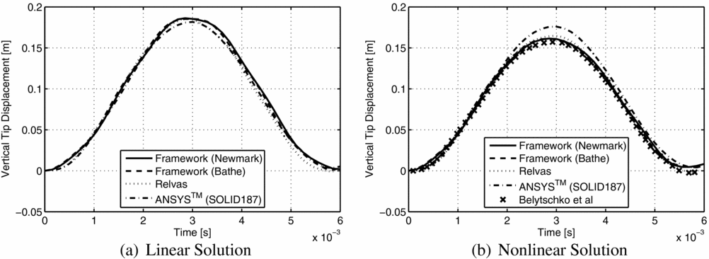
) and mesh (20 finite elements). Despite the beam shape, literature models are based on plates. So, in order to expand the comparison to other elements, linear and non-linear transient analyses were carried out in ANSYS™ using the same time step and a mesh of solid elements (SOLID187) with a 80 × 8 × 8 (length, width and height) discretisation. In Fig. 4, the different linear and non-linear transient responses measured at the beam tip are depicted for the first
 $0.006\,\text{s}$
.
Structural dynamic response, literature results are marked as Relvas(Reference Relvas46) and Belytschko et al(Reference Belytschko, Lin and Chen-Shyh10) in the legends.

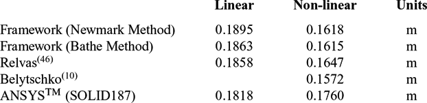
One can observe from Fig. 4 that both linear and non-linear framework solutions are in very good agreement with those found in the literature. Maximum errors under 2% and 3% were verified for linear and non-linear solutions, respectively. Despite this good agreement with the literature results, the non-linear dynamic solutions obtained using the developed framework are different from those of the solid element, mainly in terms of amplitude, which is lower (maximum errors of 8.07% and 8.26% were observed when comparing the framework results obtained using the Newmark and Bathe methods, respectively). It is worth noting that the implemented beam finite element has a different formulation (based on Euler-Bernoulli beam theory) to those of the solid element, which results in a more accentuated difference in the non-linear solution when very large deformations occur (the vertical tip displacement corresponds to more than 70% of the total beam length for the linear solution). The linear and non-linear vertical tip deflection values are summarised in Table 1.
Vertical tip deflection

2.3 Aeroelastic model
In order to perform an aeroelastic analysis, this model has to adequately couple the aerodynamic and structural solvers. To do so, a Fluid-Structure Interaction (FSI) algorithm capable of performing steady and unsteady calculations was developed.
2.3.1 FSI
The FSI methodology implemented can be classified as: (1) monolithic(Reference Hulshoff27), since the solution advances with the convergence between structural and aerodynamic solutions at a time instant in the unsteady case (or at a given load step for the steady case); and (2) loosely coupled(Reference Bazilevs, Takizawa and Tezduyar9) since the fluid and structure equations are solved separately and coupled in an interface model until convergence is reached.
This algorithm is responsible for transferring the loads from the aerodynamic panels to the structure and transferring the structural displacements to the aerodynamic panels. Usually, accurate modelling of the fluid dynamics requires a detailed mesh, while for modelling the structural dynamics, a relatively coarse mesh suffices(Reference Ballmann5). As a consequence, the two meshes are not coincidental and, therefore, a proper load and displacement transfer method is necessary.
The aerodynamic loads computed at each aerodynamic node are transferred to the structural mesh by means of generating an equivalent load system, which is applied to the closest beam finite element. Despite ensuring consistency, this approach does not guarantee energy conservation. Nevertheless, for flexible structures, such as high-aspect-ratio wings, if one ensures energy conservation, one might obtain large non-physical oscillations in the pressure force resulting in a significant negative influence on results accuracy(Reference Rixen47).
No aerodynamic mesh deformation is performed; instead, a new mesh of the deformed shape is generated for each aerodynamic calculation. This mesh is built based on the structural displacements, which are transferred to aerodynamic nodes by assuming the aerofoil cross-section as rigid, i.e. the structural nodal displacement is transmitted to the aerodynamic node by a rigid-link.
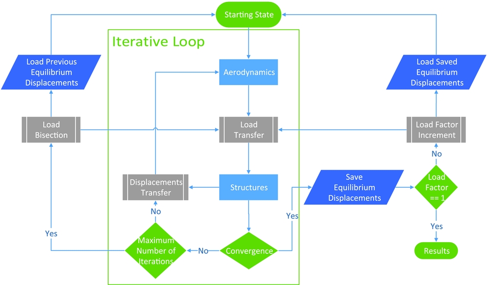
The FSI routine is an iterative process which converges when equilibrium is reached, i.e. when both displacements and loads have converged. In the steady case, the aerodynamic model is re-meshed at each equilibrium iteration. In order to facilitate convergence, a few features were included in the developed framework: firstly, in the case where convergence has not been reached, the FSI module performs a bisection of the load and displacement and starts at the previous equilibrium state (which, in the case of the bisection taking place in the first iteration, is the undeformed state); secondly, it is possible to begin with just a fraction of the total load meant to be transferred to the structure. The convergence criteria is given by,
 $$\begin{equation}
\frac{1}{NN}\sum _{i=1}^{NN}\left|\frac{d_i^n-d_i^{n-1}}{d_i^n}\right|\le 1\times 10^{-7},
\end{equation}$$
where NN and di are, respectively, the number of structural nodes and nodal displacement (displacements and rotations) i, n is the current load step and n − 1 the previous load step. Figure 5 shows the implemented FSI flowchart for static aeroelastic calculations.
Steady FSI algorithm flowchart.

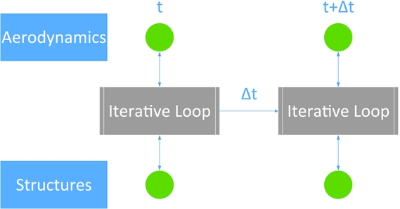
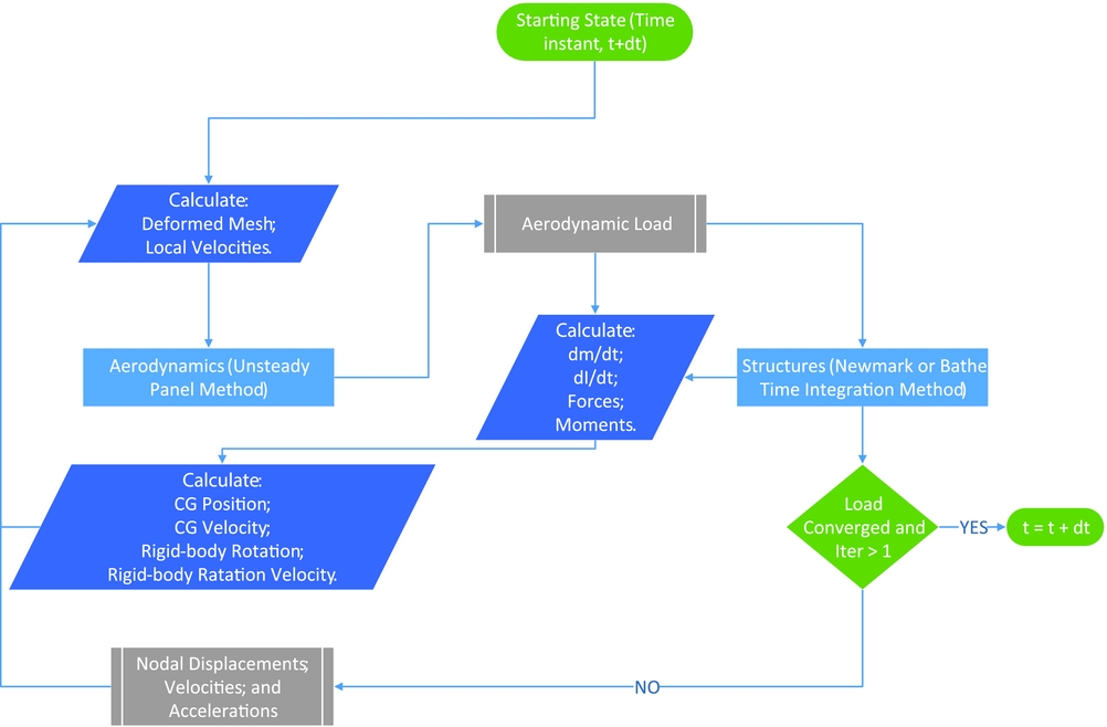
All structural time marching schemes assume the loading as a function of time is known. For an unsteady FSI analysis, this is not the case, since the aerodynamic loading at a particular time is determined by the deformed position of the wing/aircraft and by the local deformation speed influencing, for instance, the local angle-of-attack. In particular, when using an unsteady panel method, such as the one implemented, the aerodynamic loading calculation requires a re-meshing or mesh deformation procedure according to the aircraft deformation and that the local velocity at the collocation points is known. Thus, an iterative process is done in order to match the load applied to the structure with the aerodynamic load computed at the end of the load step. Figure 6 shows the implemented time marching procedure; the iterative loop box is depicted in Fig. 7.
Unsteady FSI scheme.

Unsteady FSI iterative loop.

For an initial load guess (usually equal to the load at the end of the previous time step), the procedure uses a Newmark or Bathe time integration method in the structural solver for the calculation of the nodes displacements, velocities and accelerations at the end of the time step.
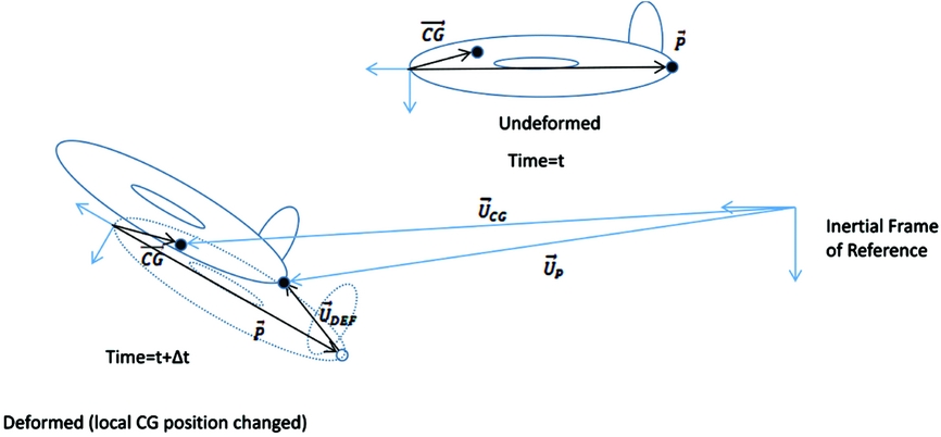
With the nodal displacements and displacement velocities available, one of two possible work flows follows, depending on the model being constrained or not. If the model is free, an intermediate step is performed in order to obtain information about the Centre of Gravity (CG) position, rigid body orientation and linear and rotation speeds by decomposing the total displacement and displacement velocities into rigid+deformation components, as depicted in Fig. 8. This decomposition allows the use of the framework for rigid body flight simulation by neglecting structural deformation. With the resultant loading from aerodynamic and other sources (e.g. propulsion and gravity), a 4th-order Runge-Kutta integration scheme with an embedded predictor-corrector scheme for aero-structural convergence is used to determine the rigid body CG position and orientation, and CG linear and rotation speeds at the end of the time step, followed by a predictor-corrector scheme used for aero-structural convergence and to determine the linear and rotational accelerations, as well as in the end of the time step. If the model is constrained (e.g. half wing clamped at the root, as is the case studied in this work) the orientation of the model is assumed fixed and the rigid body components are assumed null. In this case, the predictor-corrector scheme is used for aero-structural convergence before advancing the solution in time.
Example of mesh deformation calculation for a CG position displacement from time t to time t = t + Δt.

2.3.2 Re-meshing procedure
The re-meshing procedure is based on rigid links between structural and aerodynamic nodes, as already mentioned. The aerodynamic mesh is constructed by defining a set of points and associated aerofoil (or fuselage) shapes and shape-related parameters (e.g. chord, twist and wing-box chord-wise limits), in a piece-wise linear or other shape function approximation. These points are the ones to which the structural displacement is passed on to by a rigid link connecting them to the associated structural nodes. In the present case, the aerofoil shape is assumed to be rigid and, therefore, it is translated and rotated according to the structural deformation calculated. In the unsteady case, not only the mesh is updated according to the structural deformation but also the deformation speed is calculated for each aerodynamic panel control point, by linear interpolation of the deformation speeds calculated for the construction points in which the aerodynamic panel is between. This relative velocity is then added to zero normal flow boundary condition for the aerodynamic panel.
2.3.3 Static aeroelastic analysis
For the static aeroelastic calculations, the steady FSI algorithm, shown in Fig. 5, is employed, which calculates the linear or non-linear static equilibrium position.
2.3.4 Dynamic aeroelastic analysis
Two dynamic aeroelastic methodologies were implemented: (1) frequency domain and (2) time domain. The former consists in calculating the flutter boundary at the linear or non-linear equilibrium state (computed with the steady FSI algorithm) using the p-k method(Reference Hodges and Pierce26). In the latter, the unsteady FSI (time-marching scheme, shown in Fig. 6) is used to compute the non-linear aeroelastic deformed state in time.
NASTRAN™ was used for flutter speed calculation in the frequency domain. In this methodology, only geometric non-linearities are transmitted to the NASTRAN™ model through the generation of a deformed model and the flutter speed is computed for the static aeroelastic non-linear equilibrium state.
2.3.5 Benchmarking
An experimental aeroelastic model of a high-aspect-ratio wing with a slender body, presented by Tang and Dowell(Reference Tang and Dowell57), has been used for benchmarking non-linear aeroelastic numerical codes and was, likewise, applied here to benchmark the implemented FSI algorithm: a rectangular spar with the same inertia properties was generated with the developed tool to represent the internal structure of the wing and the slender body was modelled as a mass point with equivalent mass and inertias. The generated aerodynamic model does not take into account the aerodynamics of the slender body.
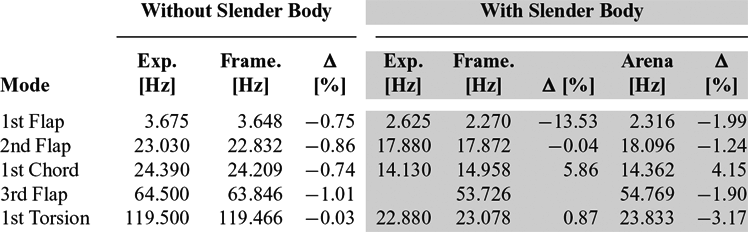
Prior to performing aeroelastic analysis, modal identification took place and the results were compared with the literature and experimental results(Reference Arena, Lacarbonara and Marzocca4). Good agreement with the numerical data of Arena et al(Reference Arena, Lacarbonara and Marzocca4) was verified, as well as with the experimental data, as can be observed in Table 2. That applies to the model with and without the slender body. It is clear that, although the addition of the slender body at the wing tip reduces all natural frequencies, the first torsion and the first chord bending modes are the ones most affected.
First 5 natural frequencies for the Framework (Frame.), Experimental (Exp.) and Arena et al(Reference Arena, Lacarbonara and Marzocca4) numerical results, with and without slender body. The Δ values represent the relative errors

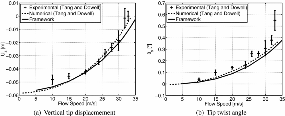
In this test case, non-linear aeroelastic solutions were computed for ten flow speeds (ranging from 5 m/s to 35 m/s), at sea level altitude and for an angle-of-attack of 1°. The results are shown in Fig. 9.
Comparison of vertical tip displacement and twist angle as a function of the flow speed with experimental and numerical results of Tang and Dowell(Reference Tang and Dowell57).

One can observe from Fig. 9(a) that the vertical tip displacement is close to the numerical and experimental data for flow speeds of up to 30 m/s. For higher speeds, the tip displacement is small, and the FSI module tends to converge faster, which together with the fact that the slender body was not included in the aerodynamic model leads to higher errors in the vertical tip displacement, when compared with the experimental data. Good agreement was found, despite the differences in the aerodynamic models (2D ONERA aerodynamic model(Reference Petot43)). It is noticeable the increase of the difference between experimental and numerical tip twist angle, i.e. when the aerodynamic of the slender body becomes more important which causes an increase of the effective angle-of-attack and, thus, an increase in vertical tip displacement. The absence of the slender body in the aerodynamic model explains the discrepancies between the developed framework results and the experimental data. In fact, the structural model closely represents the structure tested in the wind tunnel, although the absence of the slender body in the aerodynamic prevent a direct comparison between the results.
3.0 WING MODEL
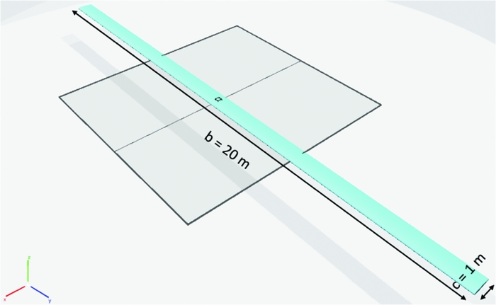
In order to investigate the effects of increasing wing aspect-ratio in flutter speed, a very simple wing model is used. The basic wing model (Fig. 10) consists of a rectangular NACA 0012 wing made of aluminum (which properties are the equal to those used in the structural model benchmarking case) with a wing span (b) of 20 m and a unitary chord (c). A wing-box layout that starts and ends, respectively, at 25% and 75% of chord, with different values for web and cap thicknesses, was selected as the wing structural model.
Basic wing model configuration.

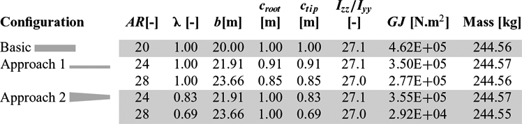
Two approaches were used to increase the wing aspect-ratio. With the goal of reaching a good comparison between wing models in mind, both the wing area (S) and wing mass were maintained yielding the same increase in wing span as aspect-ratio increases. Approach 1 consists in keeping the wing rectangular, i.e. with a taper-ratio unitary (λ = 1), and varying the chord (
 $c_{root} = c_{tip}=1,0.91,0.85\,\textrm {m}$
) and span (
 $b=20,\;21.91,\;23.66\,\textrm {m}$
) to produce three different aspect-ratios (AR = 20, 24, 28). An alternative approach, called Approach 2, was also explored, where the wing-root chord was maintained (
 $c_{root} = 1\,\textrm {m}$
), but the wing-tip chord was reduced (
 $c_{tip} = 1,\;0.83,\;0.69\,\textrm {m}$
) to generate the same three aspect-ratios and, consequently, also the taper-ratio (λ = 1, 0.83, 0.69) decreased. Thus, five different high-aspect-ratio wing configurations were considered in this work, as can be seen in Table 3.
Main characteristics of the five different wing configurations (the torsional stiffness,
 ${\bm GJ}$
, value corresponds to value at the wing tip)

In both approaches, the wing inertia ratio (Izz /Iyy ), which corresponds to a ratio between chord bending stiffness (EIzz ) and flap bending stiffness (EIyy )Footnote 1 , was maintained nearly constant. According to Tang and Dowell(Reference Tang and Dowell57), this parameter has an important impact on the flutter speed, although, due to the chord reduction, the torsional stiffness (GJ) decrease. The wing span was increased to maintain the same wing area and the internal thicknesses of the wing-box (webs and caps) were determined such that the wing mass and inertia ratio are maintained (within 1% difference). The taper-ratio reduction in the second approach did not change the inertia ratio; however, it modified other important structural properties: mainly the mass moment of inertia distribution, but also the torsional stiffness, thus changing the span-wise lift distribution. The main characteristics of the five different wing configurations are summarised in Table 3.
4.0 RESULTS
Before evaluating the aeroelastic performance of the five different aspect-ratio wings in terms of flutter speed, first aeroelastic static analyses were carried out to assess the aerodynamic and structural behaviours at the aeroelastic static equilibrium state in terms of drag polar, lift-to-drag ratio, root bending moment and natural frequencies.
The non-linear static analyses were performed considering the same flight condition for all the cases: constant airspeed of 40 m/s; sea level altitude conditions; and angle-of-attack ranging from − 4° to 10°. Airspeed and altitude were chosen such that the flow remains low subsonic and incompressible. Since the aspect-ratios considered in these studies are relatively high, the 3D effects on the lift distribution are expected to be low.
Convergence studies were performed to set both aerodynamic and structural meshes. The aerodynamic mesh consists of 210 span-wise divisions and 40 chord-wise divisions spaced in a cosine distribution. One fixed wake panel of 100 chord lengths was assigned to each span-wise division in wing chord direction. For the structural mesh, 50 non-linear beam elements uniformly distributed were used.
4.1 Aeroelastic static performance
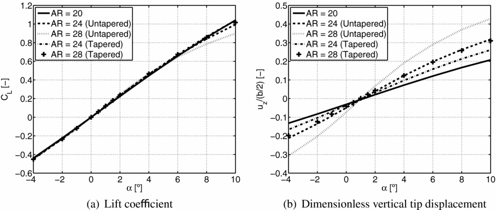
Fig. 11(a) shows the CL variation with angle-of-attack for the five different aspect-ratio wings. It can be seen that as the aspect-ratio increases, the range of linear dependence of CL with α is reduced, which is much more evident for Approach 1 than for Approach 2 (barely noticeable). This is due to the higher vertical displacements caused by a reduction on the bending stiffness (EI) on both flap and chord planes, and due to the higher incidence angles caused by torsional stiffness decrease, when the wing chord decreases and aspect-ratio increases. Both effects are much less significant for Approach 2 than for Approach 1, since, when reducing the wing taper-ratio, the impact caused by the reduction of torsional and bending stiffness towards the wing tip is lower relative to the first approach. The increase on the wing aspect-ratio causes an increase in C L α (see Fig. 11(a)) and a non-linear deformation, especially for Approach 1, as can be observed in Fig. 11(b), which depicts the dimensionless tip vertical displacement variation with α for the five wings. One can see that the higher aspect-ratio values cause higher displacements for the same α in both approaches, which is caused by the decrease on the bending stiffness and torsional stiffness as chord decreases and aspect-ratio increases (effect more evident for Approach 1).
Lift coefficient and dimensionless vertical tip displacement variations with angle-of-attack (α) and aspect ratio (AR).

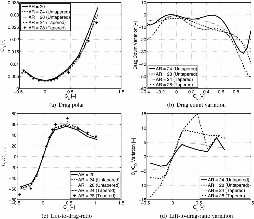
The aerodynamic performance of the non-linear aeroelastic static equilibrium states in terms of drag polar and lift-to-drag ratio is shown in Fig. 12. One can notice from Fig. 12(b) that there is a reduction of CD (measured in drag counts) for the same CL as aspect-ratio increases, with the respect to the basic configuration (AR = 20), which is in agreement with the induced drag reduction predicted by the theory. However, this reduction is highly non-linear with CL and is slightly more effective when following Approach 2. The lift-to-drag ratio plots depicted in Figs 12(c) and (d) are in agreement with what is predicted by the theory: this ratio increases as aspect-ratio increases. It is worth noting that the lift-to-drag ratio variation is equal for both approaches within a small range of low CL values (between − 0.12 and 0.18), outside this margin, the variation is higher for Approach 2.
Aerodynamic performance of five different aspect-ratio wings as a function of CL . The variation plots are the variations of CD (b) and CL /CD (d), in reference to the basic configuration (AR = 20).

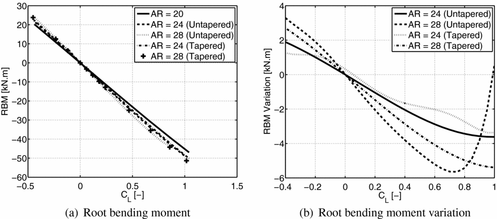
In what concerns the structural metrics, the root bending moment and the natural frequencies for the five different wing configurations were evaluated and compared. The root bending moment is a widely applied structural constraint in wing design projects and so it was used to evaluate the structural performance of the analysed wings. As expected from the theory, by increasing the wing span increase while keeping the same mass, the root bending moment value grows. This behaviour can be observed in Fig. 13, which shows the root bending moment variation in reference to the basic wing configuration (AR = 20) as a function of CL . One can also note that the tapered wings (Approach 2) present lower root bending moments than the untapered wings (Approach 1), which is mainly explained by the fact that the wing loading is smaller towards the tip for tapered wings than for the untapered wings.
Root bending moment as a function of CL for the five different wing configurations (a) and the root bending moment variation with respect to the basic configuration (AR = 20) as a function of CL .

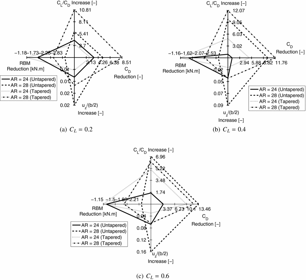
A spider chart depicting the performance of each wing relative to the basic wing configuration in terms of drag coefficient reduction (positive values correspond to a reduction), lift-to-drag ratio increase (positive values correspond to an increase), root bending moment decrease (positive values correspond to a reduction) and dimensionless vertical tip displacement increase (positive values correspond to an increase) is shown in Fig. 14 for three different lift coefficient values. The aerodynamic metrics (drag reduction and lift-to-drag increase) are always beneficial, while the structural metrics (root bending moment and dimensionless vertical tip displacement) are always prejudicial. The tapered wing with an aspect-ratio of 28 starts presenting the highest amount of drag reduction and lift-to-drag ratio increase for the lowest considered CL (CL = 0.2); although, as CL increases, the untapered wing with an aspect-ratio of 28 reduces the difference to the prior, and for the highest CL considered (CL = 0.6), it outperforms the first in aerodynamic benefit. The tapered wings always present a lower increment on the root bending moment than the untapered wings, besides exhibiting lower vertical tip displacements.
Spider charts showing the CD reduction (in drag counts), CL /CD increase, root bending moment (RBM) reduction (in kN.m) and dimensionless vertical tip displacement increase (uz (b/2)) relative to the basic wing configuration (AR = 20) for three different CL values.

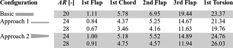
The first five undeformed mode shapes were identified and are presented in Table 4 for the five different wing configurationsFootnote 2 . One can notice that the natural frequencies associated to both flap and chord bending modes decrease as the aspect-ratio increases together with the associated reduction of flap and chord bending stiffness, respectively. The torsion natural frequency presents opposing behaviour for the two approaches: by increasing wing aspect-ratio and keeping the wing rectangular and with the same mass (Approach 1), the torsional rigidity reduces and, consequently, also this frequency decreases; by reducing the taper-ratio to increase wing aspect-ratio (Approach 2), the torsional rigidity also decreases, but the reduction of the inertia mass moment towards the wing tip causes an increase in the first torsion natural frequency.
First five natural (undeformed) frequencies (in Hz) for the five different wing configurations

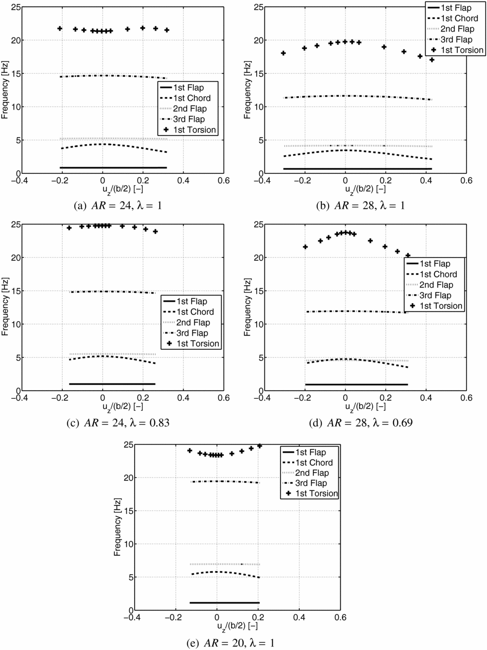
The variation of the deformed natural frequencies with dimensionless tip displacement for the five different aspect-ratio wings and for the first five natural modes of vibration is shown in Fig. 15. The values of the dimensionless tip displacements correspond to the non-linear aeroelastic equilibrium states for the flight conditions computed (a constant airspeed of 40 m/s and angles of attack ranging from − 4° to 10°). From Fig. 15: firstly, one can observe that the flap bending frequencies remain nearly constant with the tip displacement, while the first chord bending and torsional frequencies vary with the dimensionless tip displacement; secondly, one can observe that the behaviour of the natural frequencies’ variation with dimensionless tip displacement is similar for the five wings (for both approaches followed), except for the first torsion mode.
Evolution of the natural frequencies with the wing deformation.

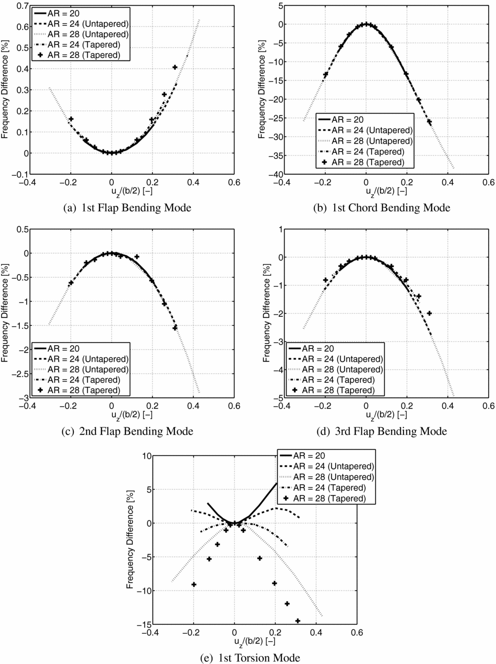
Figure 16 depicts the first five natural frequencies’ variation, relative to the corresponding undeformed natural frequencies (in percentage) as a function of dimensionless tip displacement. For the flap bending modes (Figs 16(a), (c) and (d)), the difference between undeformed and deformed natural frequencies stays below 5%. The magnitude of the differences increases as the frequency is higher, and for the second and third flap bending modes, it increases with the magnitude of the dimensionless tip displacement. For the first flap bending modes (Fig. 16(a)), the natural frequencies increase with the dimensionless tip displacement in contrast with the second (Fig. 16(c)) and third (Fig. 16(d)) flap bending modes, but the magnitude of the differences is very low and, therefore, not significant.
Evolution of the natural frequencies with the wing deformation in detail.

For the chord bending mode, Fig. 16(b) shows the results of frequency difference variation with the dimensionless tip vertical displacement. The dependence of the chord bending frequency with the chord is not significant, and by looking at the first chord bending curves, one can see that they are almost superposed for the different aspect-ratio wings, meaning that dependence on the chord is not as significant as on the tip displacement.
The results for flap and chord bending frequencies show that the two modes have similar behaviour, i.e. both curves for the different aspect-ratio wings are nearly superposed, which means that, if the inertia ratio I 1/I 2 is maintained, the vertical tip displacement is the governing factor and not the aspect-ratio or chord variation. Nevertheless, their magnitude is different: the chord bending mode presents a much higher (reaching up to 38.38% change in frequency) dependence on vertical tip displacement than the flap bending modes (a maximum change in frequency of 4.93% was achieved for the third flap bending mode). This result is in agreement with effects observed by Bhatia(Reference Bhatia12) regarding large wing deflection. It is worth mentioning that the approaches followed to increase wing aspect-ratio present the same behaviour, although the variation is slightly more smooth for the second approach (tapered wings) than for the first (untapered wings).
The results for the torsion frequency also change significantly, representing a 14.48% change in magnitude for the tapered wing with the highest aspect-ratio, as can be seen in Fig. 16(e). While for the flap and chord bending modes, the dimensionless tip displacement appears to be the main driving parameter; for torsion, a different behaviour is observed. For the basic wing configuration (AR = 20), the first torsion (deformed) frequency increases as vertical tip displacement increases; although, for higher values of aspect-ratio, other factors gain relevance, changing the trends of torsion frequency difference: first, reducing the rate of frequency increase at lower vertical tip displacements and then inverting the trend (AR = 24 for both approaches); finally, the frequency difference becomes monotonically decreasing with the vertical tip displacement (AR = 28 for both approaches).
4.2 Aeroelastic dynamic performance
The time-marching scheme described earlier was applied to calculate the flutter speed for both approaches (1 and 2). In order to determine the flutter speed, a frontal triangular wind gust profile is prescribed to excite the wing structure at the aeroelastic static equilibrium. The defined gust profile starts at 0 s and has a wind speed peak of 5 m/s and lasts for 0.05 s. The time step was carefully selected after performing a time step study, from which was observed that the most suitable value was 0.01 s. All structural analyses were carried out using the Newmark method and a predictor-corrector scheme was followed to ensure aeroelastic convergence.
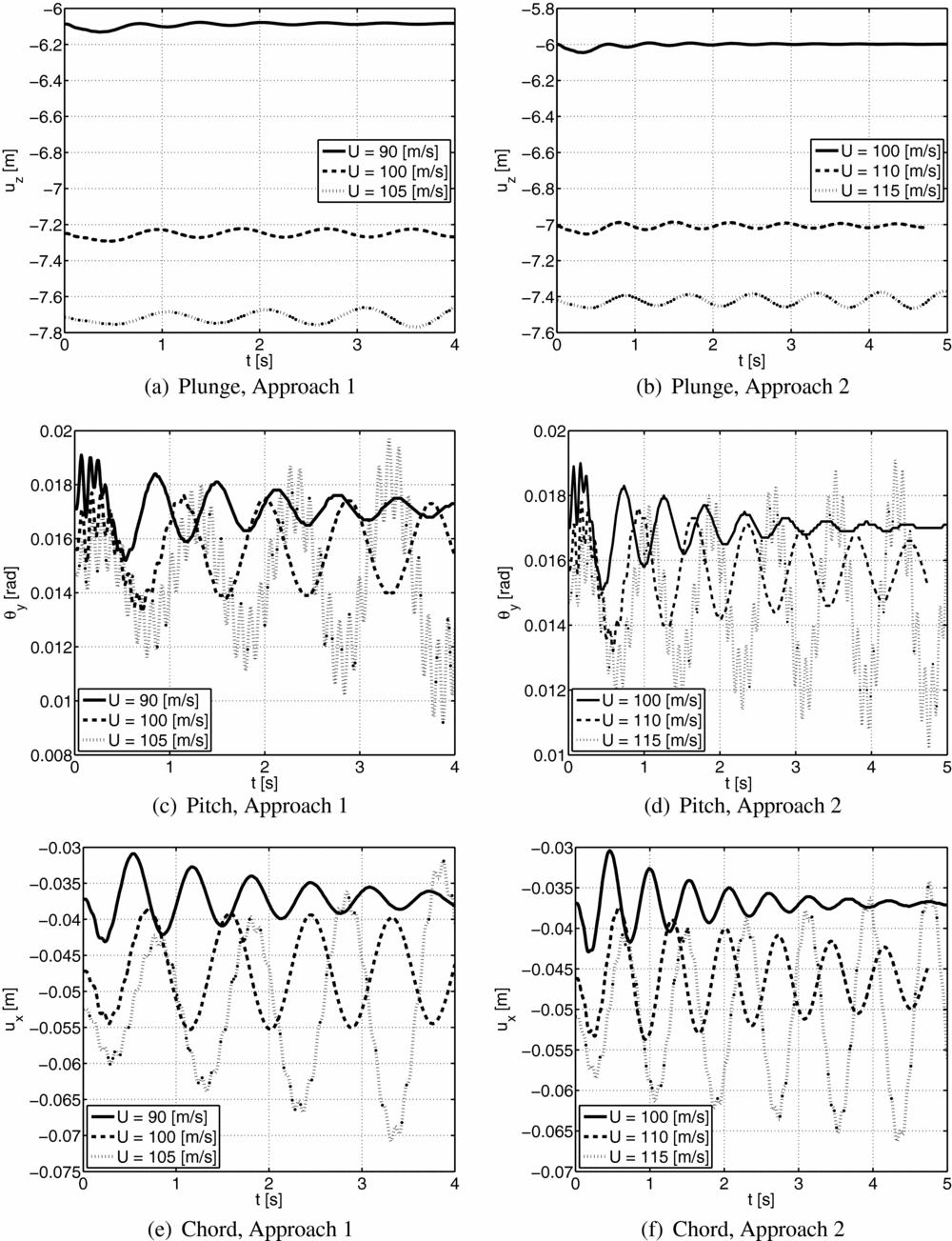
The flutter speed was estimated based on the damping of the dynamic response measure at the wing tip in plunge (vertical tip displacement, uz ), pitch (twist angle, θ y ) and chord (wing plane displacement, ux ) DOFs. By determining the damping ratio at different speeds before and after the flutter, the flutter speed is calculated through interpolation of the speed vs damping data for a zero damping ratio. An illustrative example is shown in Fig. 17 for the wings with aspect-ratio 24, where one can clearly notice: the increase of plunge, pitch and chord peaks as airspeed is increased for both approaches until the response becomes divergent; the effect of the triangular wind gust, which causes a second oscillatory response that only dissipates for speeds lower than the flutter speed. Similar plots can be drawn for the remaining wings, which were observed to present the same aeroelastic dynamic behaviour.
Dynamic response of the wings with an aspect-ratio of 24 measured at the wing tip in plunge (uz ), pitch (θ y ) and chord (ux ) DOFs for three different airspeeds.

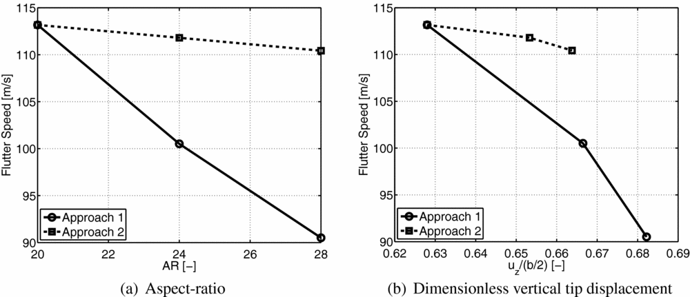
Figure 18 depicts the flutter speed values estimated for Approach 1 and 2 as a function of the aspect-ratio (a) and the dimensionless vertical tip displacement (b). One can clearly note that the flutter speed is higher for Approach 2 (tapered wings) than for Approach 1 (untapered wings) as expected, since both tip displacement and natural frequencies’ difference (between deformed and undeformed frequencies) is also lower in Approach 1. Nonetheless, the flutter speed decreases as aspect-ratio and vertical tip displacement increase for both approaches. It is also worth mentioning two interesting observations: the rate of flutter speed decrease as a function of vertical tip displacement or aspect-ratio increase is smaller for Approach 2 when compared with Approach 1; the vertical tip displacement increase appears to have a significant impact on the flutter speed decrease, especially for Approach 1.
Flutter speed as a function of aspect-ratio (a) and dimensionless vertical tip displacement (b) for Approaches 1 (Untapered Wings) and 2 (Tapered Wings).

5.0 CONCLUDING REMARKS
A non-linear aeroelastic framework with both static and dynamic modelling capabilities was developed to analyse geometric non-linear effects on high-aspect-ratio wings. Good agreement was verified when benchmarking the code with existing experimental data and high-fidelity numerical codes.
In this study, the influence of geometrical non-linearity was assessed for five comparable high-aspect-ratio wing models. Two strategies to increase wing aspect-ratio while maintaining them to be comparable (i.e. with the same wing area and mass) were followed: reducing the wing chord and increasing the wing span while keeping the wing rectangular (Approach 1); and reducing the wing taper-ratio and increasing the wing span (Approach 2). The lift slope was observed not to vary significantly for the tapered wings, while the linear dependence of CL with α was reduced by reducing the chord of the untapered wings. This effect is caused by the very high deformations observed for the rectangular wing models.
An aerodynamic and structural performance comparison was conducted by analysing four metrics (drag coefficient, lift-to-drag ratio, dimensionless vertical tip displacement and root bending moment) at different values of CL with respect to the basic configuration (AR = 20). A noticeable improvement in the aerodynamic metrics of lift-to-drag ratio and drag coefficient was verified using both approaches, as predicted by the theory, although this improvement was observed to have a non-linear dependence with CL . Regarding the structural performance, large displacements, as well as higher root bending moments, were achieved for the rectangular wings (Approach 1) and for the higher wing aspect-ratios. These are expected results since if one increases the wing span and at the same time maintains the total mass, the root bending moment increases; and by tapering the wing, the load distribution at the wing becomes smaller towards the tip, thus, reducing the root bending moment.
The flap and chord bending modes’ frequencies for the models depend mainly on the vertical tip displacement, with the curves almost superposed. The first torsion mode does not show a similar behaviour to the one predicted for the bending modes; this mode was found to depend not only on the displacements, but also on important parameters, such as torsional stiffness distribution and mass inertia moment in the deformed state.
The flutter speed was estimated based on the wing response measured at the tip in terms of plunge, pitch and chord DOFs to a prescribed triangular wind gust. From this study, it was observed that the tapered wings exhibit higher flutter speeds than the untapered wings, which vary more with the aspect-ratio and vertical tip displacement. Nevertheless, both approaches present the same behaviour, the flutter speed decreases as aspect-ratio increases and as dimensionless vertical tip displacement increases.
In general, the contribution of the geometric non-linearities (in terms of large deformations) was determinant to the flutter speed calculations, which confirms the importance of designing and optimising a flexible wing using a non-linear approach. From what was observed for wings with aspect-ratio above 20, large deformations decrease the safety margin for flight operations.
ACKNOWLEDGEMENTS
The presented work was carried out as part of the EU Seventh Framework Program Project NOVEMOR and the authors thank the European Commission for funding this research (Grant Agreement 285395). Additional support was also provided by the National Science and Engineering Research Council in Canada.